Symmetry and optical selection rules in graphene quantum dots

Abstract

Graphene quantum dots (GQD’s) have optical properties which are very different from those of an extended graphene sheet. In this Article we explore how the size, shape and edge–structure of a GQD affect its optical conductivity. Using representation theory, we derive optical selection rules for regular–shaped dots, starting from the symmetry properties of the current operator. We find that, where the x– and y–components of the current operator transform with the same irreducible representation (irrep) of the point group — for example in triangular or hexagonal GQD’s — the optical conductivity is independent of the polarisation of the light. On the other hand, where these components transform with different irreps — for example in rectangular GQD’s — the optical conductivity depends on the polarisation of light. We carry out explicit calculations of the optical conductivity of GQD’s described by a simple tight–binding model and, for dots of intermediate size, find an absorption peak in the low–frequency range of the spectrum which allows us to distinguish between dots with zigzag and armchair edges. We also clarify the one–dimensional nature of states at the van Hove singularity in graphene, providing a possible explanation for very high exciton–binding energies. Finally we discuss the role of atomic vacancies and shape asymmetry.

I Introduction

Graphene, a single sheet of carbon atoms arranged in a honeycomb lattice, became experimentally accessible in 2004 through perhaps the most innovative use of scotch tape in the 21st century Novoselov (2004); Novoselov et al. (2005). The first of the many surprises of this “wonder material” was that it could be seen at all, using nothing more than an optical microscope Nair et al. (2008). And in fact, the large, universal, and approximately constant optical response of graphene in the visible spectrum is a signature of one of its other remarkable properties — electrons with a relativistic “Dirac” dispersion Ando et al. (2002); GUSYNIN et al. (2007); Ziegler (2007); Min and MacDonald (2009); Stauber et al. (2008); Yuan et al. (2011a); Buividovich and Polikarpov (2012).

Graphene is also a very good conductor of DC electric current Novoselov et al. (2005); Geim and Novoselov (2007); Miao et al. (2007). However in this case, the conductivity measured in experiment is found to depend on the boundaries of the graphene sheet Katsnelson (2006); Tworzydło et al. (2006); Ryu et al. (2007), a fact which highlights the topological character of graphene’s electronic statesDas Sarma et al. (2011); Kotov et al. (2012). Boundary effects are even more pronounced in graphene nanostructures referred to as “graphene quantum dots” (GQD’s). GQD’s have a discrete energy spectrum, and can be viewed as large, sp²–bonded, carbon molecules, with electronic states which depend on the size, shape and symmetry of the dot Silva et al. (2010); Güçlü et al. (2014, 2010).

The possibility of engineering the energy spectrum of a GQD, and therefore its optical properties, has suggested potential applications in fields ranging from quantum computation to solar energy Zhu et al. (2011); Luk et al. (2012); Son et al. (2012); Konstantatos et al. (2012); Kim et al. (2012); Jin et al. (2013); Zhang et al. (2015); Roy et al. (2015); Umrao et al. (2015); Jiang Wu (2014). A range of different fabrication techniques are now available for GQD’s Coraux et al. (2009); Lu et al. (2011); Li et al. (2011); Mohanty et al. (2012); Olle et al. (2012); Yan et al. (2012); Müllen (2014); Wang et al. (2014). However, tailoring the properties of a GQD to a specific application requires the ability to fabricate dots with the desired shape, or to post–select for dots with a given shape after fabrication. In either case, understanding the relationship between the size and shape of the dot, and its optical properties is paramount.

In this Article, we explore how the size, shape and edge–geometry of a GQD combine to determine its optical conductivity, paying particular attention to the symmetry of the dot, and the optical selection rules which follow from it. Considering regular GQD’s with a range of different shapes, we first examine how different point–group symmetries lead to different optical selection rules. We find that selection rules depend on the way in which the different components of the current operator transform under the symmetries of the dot. Where both components of the current operator, $\hat{\mathpzc{J}}^{x}$ and $\hat{\mathpzc{J}}^{y}$, transform with the same irreducible representation (irrep) of the point group — for example in triangular dots — we find that the optical conductivity does not depend on the polarization of the incident light. On the other hand, where the different components of the current operator transform under different irreps — for example in rectangular dots — the optical conductivity does depend on the polarization of the incident light. This result is illustrated through explicit, numerical calculations of the optical conductivity of regular GQD’s within a simple tight–binding model.

The same numerical approach is used to explore how the optical properties of a GQD evolve into those of a graphene sheet, as the size of the dot is increased. Here we find that edge–geometry plays an important role, with zigzag edges contributing a strong, additional feature to the optical conductivity within the visible spectrum, for GQD’s of linear dimension $L>10\ \text{nm}$, with spectral weight which scales as $1/L$. This feature is absent in GQD’s with armchair edges, allowing a direct distinction between dots with different edge–types for dots of intermediate size.

We also examine how the strong peak in the optical conductivity of graphene in the ultraviolet, at $\hbar\omega\sim 4.7~{}\text{eV}$ [Eberlein et al., 2008; Mak et al., 2011], evolves out of the spectrum of a GQD. Within a tight–binding model, this peak occurs at twice the energy of the hopping integral, and is associated with a Van Hove singularity in the single–particle density of states Castro Neto et al. (2009). A very similar feature is observed in the optical conductivity of GQD’s, where it can be traced to a highly–degenerate set of electronic states with one–dimensional character. The one–dimensional nature of these states suggest a possible explanation for the high binding–energies of excitons in graphene Yang et al. (2009); Kravets et al. (2010); Mak et al. (2011); Chae et al. (2011); Matković et al. (2012).

Finally, we investigate the optical properties of GQD’s with irregular shape and disorder, in the form of vacancies in the lattice. In this case, we find a polarization–dependent optical conductivity which depends on the details of each individual, asymmetric dot. We also find new optical features arising from vacancies in the lattice. Averaging over an ensemble of dots restores the polarization–independence of bulk graphene, but does not eliminate new features coming from vacancies.

While graphene is a new phenomenon, the study of the optical properties of two–dimensional (2D) materials has a long history. Theoretical studies of the optical conductivity in 2D systems date back roughly 70 years in the context of single graphite layers Wallace (1947), zero–gap semiconductors Fradkin (1986) and d–wave superconductors Lee (1993). Nevertheless, studies explicitly in graphene experienced a sharp increase after its experimental realisation Castro Neto et al. (2009); Peres (2010); Das Sarma et al. (2011); Kotov et al. (2012). The existence of Dirac cones in the dispersion relation classifies graphene as a semimetal with novel features like the presence of massless Dirac fermions Novoselov et al. (2005), an absence of backscattering from electrostatic barriers known as the Klein paradox Katsnelson (2006) and an unconventional integer quantum Hall effect Novoselov et al. (2005); Zhang et al. (2005); Gusynin and Sharapov (2005), to name but a few.

The transport and optical properties of graphene have also attracted considerable interest. An important prediction, which predates the discovery of graphene, is that its DC conductivity without disorder takes on the value of Shon and Ando (1998); Ando et al. (2002); Noro et al. (2010)

$$\sigma^{DC}_{theo}=\frac{4}{\pi}\frac{e^{2}}{h}\;.$$ (1)

Early experiments reported values which were larger than this prediction by a factor of $\pi$, a fact which became known as the “mystery of the missing pi” Novoselov et al. (2005); Geim and Novoselov (2007). Later studies explained in theory Katsnelson (2006); Tworzydło et al. (2006); Ryu et al. (2007), and confirmed in experiment Miao et al. (2007), that the value of $\sigma^{DC}$ strongly depends on the boundary conditions of the graphene sheet, highlighting the important role of topology in graphene’s electronic states. Disorder and interactions have been argued to also play a role Ando et al. (2002).

Perhaps the most striking feature of graphene’s optical conductivity is its universal value

$$\sigma_{0}=\frac{\pi}{2}\frac{e^{2}}{h}$$ (2)

over a wide range of frequencies which include the visible spectrum Ando et al. (2002); Ziegler (2007); Min and MacDonald (2009); Stauber et al. (2008); Yuan et al. (2011a); Buividovich and Polikarpov (2012). This universal optical conductivity is observed in experiments Nair et al. (2008); Mak et al. (2008); Kuzmenko et al. (2008); Mak et al. (2011); Gogoi et al. (2012), and falls within the visible spectrum, making it possible to see a single layer of carbon atoms using only an optical microscope Nair et al. (2008). The optical conductivity of graphene remains nearly frequency–independent across the visible spectrum in the presence of (weak) disorder Ostrovsky et al. (2006); Peres et al. (2006). However, stronger disorder can lead to deviations from the universal value [Eq. (2)], and contribute an additional peak at finite–energy Yuan et al. (2011a).

The other striking feature of the optical conductivity of graphene is a strong, asymmetric peak at energies $\hbar\omega\sim 4.7\ \text{eV}$ Eberlein et al. (2008); Mak et al. (2011), with a Fano resonance–like line–shape Chae et al. (2011). This peak is seen in electron loss spectroscopy Eberlein et al. (2008) and spectroscopic ellipsometry Kravets et al. (2010) as well as in optical absorption Kravets et al. (2010), transmission Chae et al. (2011) and reflection Mak et al. (2011); Lee et al. (2011). A similar peak is seen in calculations based on a non-interacting tight–binding model, which can be attributed to a van Hove singularity in the density of states (DOS) Stauber et al. (2008). Once electron-electron interactions are taken into account, this peak is redshifted by $\Delta=400$ – $600$ meV, which is attributed to an excitonic state strongly coupled to a band continuum Yang et al. (2009); Yuan et al. (2011b); Kravets et al. (2010); Mak et al. (2011); Chae et al. (2011); Matković et al. (2012).

The optical properties of graphene change dramatically, once its electrons are spatially–confined within a nanostructure. Recently, there has been growing interest in the properties of nanoscale flakes of graphene, commonly referred to as graphene quantum dots (GQD’s), graphene nanoislands Olle et al. (2012), or nanographene Yamamoto et al. (2006). This research has also been motivated by potential applications in quantum computing Trauzettel et al. (2007), bioimaging Zhu et al. (2011); Jin et al. (2013); Roy et al. (2015); Umrao et al. (2015), LEDs light converters Luk et al. (2012); Son et al. (2012), photodetectors Konstantatos et al. (2012); Zhang et al. (2015), and organic solar cells Jiang Wu (2014). GQD’s can be synthesized in several ways, e.g. via fragmentation of C₆₀ molecules Lu et al. (2011), nanoscale cutting of graphite combined with exfoliation Mohanty et al. (2012), chamber pressure chemical vapor deposition (CP–CVD) Yan et al. (2012) and controlled decomposition of hydrocarbons Olle et al. (2012). Furthermore, scanning tunneling microscopy (STM) measurements confirmed the confinement of electronic states in GQD’s Ritter and Lyding (2009); Hämäläinen et al. (2011); Subramaniam et al. (2012); Jolie et al. (2014); Güçlü et al. (2014) and motivated further theoretical studies.

Much like graphene nanoribbons Castro Neto et al. (2009), graphene quantum dots exhibit metallic or insulating behavior depending on the type of their edges, namely zigzag or armchairZarenia et al. (2011). GQD’s with triangular geometry and zigzag edges show zero energy edge states Ezawa (2007); Potasz et al. (2010), leading to magnetic effects as edge–state magnetization Zhang et al. (2008); Güçlü et al. (2009); Potasz et al. (2012) and spin blockade Güçlü and Hawrylak (2013). Studies of optical properties of GQDs have shown signatures of edge states Yamamoto et al. (2006), excitonic effects on the optical absorption spectrum Yang et al. (2007); Güçlü et al. (2010); Ozfidan et al. (2014) and edge–dependent selection rules in triangular dots Akola et al. (2008).

Despite the huge advances made in manufacturing GQD’s, there are still obstacles to overcome towards a complete control of size, geometry and edge type. It is in this context that we revisit the question of how size, shape and edge geometry affect the optical properties of GQD’s paying particular attention to the shape of the dots. We do not explicitly take interactions between electrons into account, but instead emphasize optical selection rules which are entirely determined by symmetry, and therefore independent of the details of model Heine (1960); Landau and Lifshitz (1977); Tinkham (2003); Weyl (1950); Wagner (2001); Jones (1998).

In order to be able to compare with predictions obtained in the thermodynamic limit, we also calculate the optical conductivity within a simple tight–binding model, which is known to give a good description of many of the properties of bulk graphene Castro Neto et al. (2009). This makes it possible to explore a large range of dot sizes, and to address issues which are not determined by symmetry alone. However, this broader view comes at the expense of neglecting correlation effects, which can be significant Kotov et al. (2012).

The remainder of this Article is structured as follows:

In Section II we briefly review the calculation of the optical conductivity $\sigma_{\alpha}(\omega)$ within linear–response theory. We discuss the role of symmetry in the determining optical selection rules for a general many–electron wave function. We also introduce a simple, non-interacting tight–binding model, and describe how this can be used to make explicit predictions for the optical conductivity of a GQD of given size and shape.

In Section III we use group theory to analyse the optical selection rules found in GQD’s with triangular, hexagonal and rectangular shape. Each of these GQD’s can be classified according to a different point–group, with associated irreps. We find that, where the in–plane components of the current operator, $\mathpzc{J}_{x}$ and $\mathpzc{J}_{y}$, transform under the same irrep, the optical conductivity of the GQD, $\sigma_{\alpha}(\omega)$, does not depend on the polarization of the incident light. On the other hand, where $\mathpzc{J}_{x}$ and $\mathpzc{J}_{y}$ transform under different irreps, the optical conductivity is polarisation–dependent. We illustrate these results for non–interacting electrons by making explicit comparison with the tight–binding model introduced in Section II.

In Section IV we use the same tight–binding model to explore the way in which the optical properties of a GQD with a given shape and edge structure evolve into those of an infinite graphene sheet. We find that qualitative differences persist between GQD’s with zigzag and armchair edges, even for dots with linear–dimension $>10\text{nm}$. This suggests that optical measurements may prove a useful way to distinguish GQD’s of different edge-types.

In Section V we identify one–dimensional wave functions at energies of the Van Hove singularity of graphene, within the tight–binding model introduced in Section II This reduced dimensionality provides a possible explanation for the unusually high binding–energies of excitons, seen in experiments of graphene Yang et al. (2009); Kravets et al. (2010); Mak et al. (2011); Chae et al. (2011); Matković et al. (2012).

In Section VI we discuss irregular GQD’s and present how vacancies and asymmetry affect their optical conductivity, within the same tight–binding model. While sample averaging over many randomly shaped asymmetric dots weakens edge-effects and recovers the optical conductivity of graphene, vacancies in the bulk cause additional features similar to those seen in GQD’s with zigzag edges.

We conclude in Section VII with a summary of our results, and a discussion of potential future avenues for research.

II Theory of optical conductivity

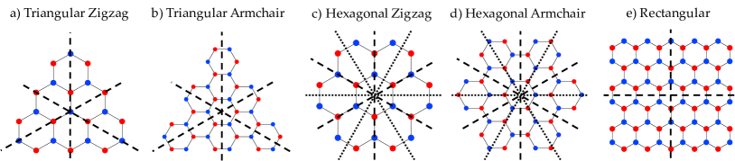
Figure 1: Regular–shaped graphene quantum dots (GQD’s) considered in this Article. (a) Triangular zigzag, (b) triangular armchair, (c) hexagonal zigzag, (d) hexagonal armchair, and (e) rectangular. Triangular and hexagonal dots have symmetries described by the non–abelian point groups $C_{3v}$ and $C_{6v}$, respectively, while rectangular dots have an abelian point group $C_{2v}$. Dotted lines represent in–plane mirror axes, while the rotation axis (not shown) is located at the centre of each dot, perpendicular to the plane of the dot.

II.1 Kubo formula and the role of symmetry

In what follows we motivate the analysis of optical selection rules in terms of the symmetries of a GQD, starting from the Kubo formula for the optical conductivity. The crucial facts will be that a) optical selection rules are determined by the matrix elements of the current operator between the different (many–body) eigenstates of the dot, and b) this current operator transforms like a polar vector under the symmetries of the dot.

Our chief measure of the optical properties of a GQD will be its optical conductivity. Formally, this is defined through

$$\mathpzc{J}^{\alpha}(\vec{q},\omega)=\sum_{\beta}\sigma_{\alpha\beta}(\vec{q},\omega)E^{\beta}(\vec{q},\omega)\;,$$ (3)

where $\sigma_{\alpha\beta}(\vec{q},\omega)$ is the optical conductivity, and $\mathpzc{J}^{\alpha}(\vec{q},\omega)$ is the current which flows as a result of an applied electric field $E^{\beta}(\vec{q},\omega)$, with frequency $\omega$, and direction $\alpha,\beta=x,y,z$. The full tensor for the optical conductivity, $\sigma_{\alpha\beta}(\vec{q},\omega)$, can be calculated within linear response theory, using a Kubo formula Mahan (2000). However for the purposes of the present study, we can make a number of simplications.

Firstly, we set $\vec{q}=0$, since the wavelength of light at the relevant frequencies is much larger than the size of the GQD. And, since GQD’s are two–dimensional, we need only to consider the two–dimensional current

$$\vec{\mathpzc{J}}=(\mathpzc{J}^{x},\mathpzc{J}^{y})\;,$$ (4)

and the in–plane components of the electric field

$$\vec{E}=(E^{x},E^{y})\;.$$ (5)

We further assume that time–reversal symmetry remains unbroken, in which case it is sufficient to only consider the diagonal part of the optical conductivity

$$\sigma_{\alpha}(\omega)=\sigma_{\alpha\beta}(\omega)\delta_{\alpha\beta}\;,$$ (6)

such that

$$\mathpzc{J}^{\alpha}(\omega)=\sigma_{\alpha}(\omega)E^{\alpha}(\omega)\;,$$ (7)

with $\alpha=x,y$. And, since the temperatures of experiment are generally small compared with the energy–scales of the dot, we further restrict our considerations to the real part of the optical conductivity, at temperature $T=0$. Both of these conditions can be relaxed at will.

With all of these restrictions in place, the Kubo formula for $\sigma_{\alpha}(\omega)$ reduces to the expectation value of the retarded, two–particle correlation function of the current operator $\hat{\mathpzc{J}}^{\alpha}(t)$, calculated within the full, many–electron ground state $|\psi_{0}\rangle$, such that

$$\text{Re}\big{[}\sigma_{\alpha}(\omega)\big{]}$$

$$=\text{Re}\left[\frac{1}{A}\frac{1}{\hbar\omega}\int_{0}^{\infty}dt\ e^{i\omega t}\ \langle\psi_{0}|\big{[}\hat{\mathpzc{J}}^{\dagger\alpha}(t),\hat{\mathpzc{J}}^{\alpha}(0)\big{]}|\psi_{0}\rangle\right]\;,$$

(8)

where $A$ is the area of the dot.

Up to this point we have not placed any restriction on the model used to describe the GQD. Quite generally, we can consider this to be described by any Hamiltonian $\hat{\mathpzc{H}}$, which respects the symmetries of a given dot. The many–electron eigenstates of this Hamiltonian

$$\hat{\mathpzc{H}}|\Psi_{n}\rangle =E_{n}|\Psi_{n}\rangle\;,$$ (9)

will also, automatically, respect the symmetries of the dot, since all symmetry operators must commute with $\hat{\mathpzc{H}}$. And we can use the completeness of these eigenstates to express Eq. (8) as

$$\text{Re}\big{[}\sigma_{\alpha}(\omega)\big{]}=\lim_{\gamma\to 0}\ \frac{2\gamma\hbar}{A}\frac{1}{\hbar\omega}\sum_{n}|\mathpzc{J}^{\alpha}_{n0}|^{2}\delta(\hbar\omega-E_{n0})$$

(10)

where

$$\mathpzc{J}^{\alpha}_{nm}=\langle\Psi_{n}\mid\hat{\mathpzc{J}}^{\alpha}\mid\Psi_{m}\rangle\;,$$ (11)

are the matrix elements of the current operator $\hat{\mathpzc{J}}$ from one many–body state to another, and

$$E_{nm}=E_{n}-E_{m}$$ (12)

is the energy of the associated optical transition.

It follows from Eq. (10) that the details of the optical response of a given GQD will depend on the precise form of the current operator $\hat{\mathpzc{J}}^{\alpha}$, and on the detailed form of the many–electron eigenstates $|\Psi_{n}\rangle$, which can generally only be found approximately. None the less, it is possible to make some statements about $\sigma_{\alpha}(\omega)$ without seeking a full solution for $|\Psi_{n}\rangle$. In particular, the optical selection rules which govern the polarisation–dependence of $\sigma_{\alpha}(\omega)$ depend only on the way in which the current operator $\hat{\mathpzc{J}}^{\alpha}$ , and the many–electron eigenstates $|\Psi_{n}\rangle$, transform under the symmetries of the dot [Weyl, 1950; Heine, 1960; Landau and Lifshitz, 1977; Tinkham, 2003; Wagner, 2001; Jones, 1998]. Simply put, the matrix element

$$\mathpzc{J}^{\alpha}_{nm}=\langle\Psi\mid\Psi^{\prime}\rangle\;,$$ (13)

[cf. Eq. (11)] must vanish if the ket

$$\mid\Psi^{\prime}\rangle=\hat{\mathpzc{J}}^{\alpha}\mid\Psi_{m}\rangle\;,$$ (14)

has a different symmetry from the bra

$$\langle\Psi\mid=\langle\Psi_{n}\mid\;.$$ (15)

It follows that identifying allowed optical transitions reduces to an exercise in symmetry analysis for the state $\mid\Psi^{\prime}\rangle$, created by the action of the polar vector $\hat{\mathpzc{J}}^{\alpha}$, on an eigenstate $\mid\Psi_{m}\rangle$, within a GQD of given shape. This is pursued in Section III, for the different GQD’s illustrated in Fig. 1.

II.2 Optical Conductivity of a GQD within the tight–binding model

Many-body interactions can have significant effects in the electronic properties of graphene Kotov et al. (2012), and will also have impact on the optical spectra of GQD’s. None the less, as discussed in Section II.1, above, optical selection rules are a special case, determined by symmetry alone. For this reason it is instructive to calculate the optical conductivity $\sigma_{\alpha}(\omega)$ explicitly for a non–interacting GQD, where optical transitions can be discussed in terms of the energy levels for individual electrons. Doing so also gives us a handle on the evolution of optical conductivity with the size of the GQD, and enables us to approach questions which are not determined by symmetry alone. The framework needed to do this is introduced below.

A good starting point to understand many of the electronic properties of graphene is the simple tight–binding model Wallace (1947); Castro Neto et al. (2009); Kotov et al. (2012):

$$\hat{\mathpzc{H}}_{0}=-t\sum_{\langle ij\rangle,s}\big{(}\hat{\mathpzc{a}}^{\dagger}_{i,s}\hat{\mathpzc{b}}_{j,s}+\hat{\mathpzc{b}}^{\dagger}_{j,s}\hat{\mathpzc{a}}_{i,s}\big{)}\;,$$ (16)

where $t$ is a hopping parameter and the sum on $\langle ij\rangle$ runs over all nearest–neighbour bonds on the honeycomb lattice. The operators $\hat{\mathpzc{a}}^{\dagger}_{i,s}$ ($\hat{\mathpzc{b}}^{\dagger}_{j,s}$) and $\hat{\mathpzc{a}}_{i,s}$ ($\hat{\mathpzc{b}}_{j,s}$) respectively create and annihilate electrons with spin $s=\uparrow,\downarrow$ at site $i$ ($j$) of sub–lattice $\mathpzc{a}$ ($\mathpzc{b}$). To describe a finite–sized system such as a GQD (Fig. 1), we assume zero hopping beyond the edges of the dot (open boundaries), which in real systems may be realized by passivating dangling bonds with hydrogen atoms.

In the case of the tight–binding model $\hat{\mathpzc{H}}_{0}$ [Eq. (16)], it is sufficient to consider single–electron eigenstates $|\psi_{n,s}\rangle$, with energy $\epsilon_{n}$, satisfying

$$\hat{\mathpzc{H}}_{0}|\psi_{n,s}\rangle =\epsilon_{n}|\psi_{n,s}\rangle\;.$$ (17)

These single–electron eigenstates can in turn be written as

$$|\psi_{n,s}\rangle = \sum_{i}c_{i,n,s}|\phi_{i,s}\rangle\;,$$ (18)

where the coefficients

$$c_{i,n,s}=\langle\psi_{n,s}|\phi_{i,s}\rangle$$ (19)

can be expressed in terms of the local atomic states through

$$\langle{\vec{r}}\ |\ \phi_{i,s}\rangle=\phi_{i,s}(\vec{r})=w(\vec{r}-\vec{R}_{i})\chi_{s}\;,$$ (20)

a Wannier orbital $w(\vec{r}-\vec{R}_{i})$ with

$$\chi_{\uparrow}=\left(\begin{array}[]{c}1\\ 0\end{array}\right)\;,\;\chi_{\downarrow}=\left(\begin{array}[]{c}0\\ 1\end{array}\right)$$ (21)

spinors representing the electron’s spin degree of freedom.

The most commonly–quoted measure of the single–electron properties is the density of states (DOS), given here by

$$g(\epsilon)=\lim_{\gamma\to 0}\frac{\gamma}{\pi}\sum_{n=1}^{N}\frac{1}{(\epsilon-\epsilon_{n})^{2}+\gamma^{2}}=\sum_{n=1}^{N}\delta(\epsilon-\epsilon_{n})\;,$$ (22)

where the sum $\sum_{n=1}^{N}$ runs over all possible single–electron eigenstates of a dot with $N$ sites. For purposes of plotting the DOS, it is convenient to work with a finite value of $\gamma$. This is equivalent to convoluting the DOS with a normalised Lorentzian, of full–width at half–maximum $2\gamma$.

It is also possible to calculate the optical conductivity within the tight–binding model $\hat{\mathpzc{H}}_{0}$ [Eq. (16)], starting from the Kubo formula, Eq. (8). An essential ingredient for this analysis is the correct form of the current operator $\hat{\mathpzc{J}}^{\alpha}$. Since electrical charge is a conserved quantity, the form of the current operator is determined by the equation of continuity for tight–binding electrons on a lattice. And the equation of continuity, in turn, is determined by the structure of $\hat{\mathpzc{H}}_{0}$. It follows that the correct form of the current operator is given by Cabib and Kaplan (1973); KUZEMSKY (2011)

$$\hat{\mathpzc{J}}^{\alpha}=-it\Big{(}\frac{e}{\hbar}\Big{)}\sum_{ij,s}\big{(}R^{\alpha}_{i}-R^{\alpha}_{j}\big{)}\big{(}\hat{\mathpzc{a}}^{\dagger}_{i,s}\hat{\mathpzc{b}}_{j,s}-\hat{\mathpzc{b}}^{\dagger}_{j,s}\hat{\mathpzc{a}}_{i,s}\big{)}\;,$$ (23)

where $R^{\alpha}_{i}$ is the $\alpha$–component of the position vector to the lattice site $i$. We note that making an inconsistent choice of the current operator can lead to incorrect values of the optical conductivity, and in particular a deviation from the universal value in Eq. (2).

For purposes of calculation, we will use Eq. (19) to express the current operator $\hat{\mathpzc{J}}^{\alpha}$ in terms of the basis $|\phi_{i,s}\rangle$

$$\mathpzc{J}^{\alpha}_{nm}=-it\Big{(}\frac{e}{\hbar}\Big{)}\sum_{ij}c^{*}_{ni}c_{mj}(R^{\alpha}_{i}-R^{\alpha}_{j})\;,$$ (24)

where, for brevity, we drop spin indices and write

$$c_{in}=c_{in,s}\;.$$ (25)

It follows from the general result, Eq. (10), that the real part of the optical conductivity is given by

$$\text{Re}\big{[}\sigma_{\alpha}(\omega)\big{]}=\lim_{\gamma\to 0}\ \frac{2\gamma}{\omega A}\sum_{nm}|\mathpzc{J}^{\alpha}_{mn}|^{2}\frac{f(\epsilon_{m})-f(\epsilon_{n})}{(\hbar\omega-\epsilon_{nm})^{2}+\gamma^{2}}\;,$$ (26)

where

$$\epsilon_{nm}=\epsilon_{n}-\epsilon_{m}\;,$$ (27)

and the Fermi function $f(\epsilon_{n})$ should be evaluated at $T=0$. We note that the numerical results for $\sigma_{\alpha}(\omega)$ presented in this Article have been calculated for a small but finite value of $\gamma$, mimicking the finite lifetime of electronic states.

II.3 Optical conductivity of an infinite graphene sheet within the tight–binding model

For many purposes, it is also interesting to compare the optical response of a GQD with that of an infinite graphene sheet. Within the tight–binding model, we can evaluate this by imposing periodic boundary conditions on the lattice, and consider its thermodynamic limit with $N\to\infty$. The result follows from Eq. (26) : for $T=0$, in the limit $q\to 0$, transitions are only allowed between states with the same crystal momentum and we find, consistent with the literatureBuividovich and Polikarpov (2012),

$$\text{Re}\big{[}\sigma_{\alpha}(\omega)\big{]}=\lim_{\gamma\to 0}\ \frac{1}{3\sqrt{3}a^{2}}\frac{t^{2}e^{2}}{\hbar^{2}}\frac{\gamma}{\omega}\frac{1}{N}\sum^{N}_{k}\frac{|\big{(}\vec{\mu}_{k}\big{)}_{\alpha}\nu_{k}^{*}+\big{(}\vec{\mu}_{k}^{*}\big{)}_{\alpha}\nu_{k}|^{2}}{|\nu_{k}|^{2}}\\ \Bigg{[}\frac{1}{(\hbar\omega-2t|\nu_{k}|)^{2}+\gamma^{2}}-\frac{1}{(\hbar\omega+2t|\nu_{k}|)^{2}+\gamma^{2}}\Bigg{]}\ ,$$ (28)

where the $\sum_{k}$ runs over all $k$–values in the Brillouin zone,

$$\nu_{k}=\sum\limits_{j=1}^{3}e^{i\vec{k}\vec{\delta}_{j}}\quad,\quad\vec{\mu}_{k}=\sum\limits_{j=1}^{3}\vec{\delta}_{j}e^{i\vec{k}\vec{\delta}_{j}}\ ,$$ (29)

and the lattice vectors $\vec{\delta}_{j}$ are given by

$$\vec{\delta}_{1}=\frac{a}{2}\{-\sqrt{3},-1\}\;,\;\vec{\delta}_{2}=\frac{a}{2}\{\sqrt{3},-1\}\;,\;\vec{\delta}_{3}=a\big{\{}0,1\}\;,\;$$

where $a$ is the lattice constant. We return to this result in Fig. 6 of Sec. IV.

III The role of symmetry

Graphene quantum dots (GQD’s) with regular shapes can be considered as macroscopic molecules, classified by their point–group symmetry. And, as with conventional molecules, different point groups lead to different optical selection rules, and therefore to different optical properties [cf. Section II.1]. In the following Section we use representation theory to derive the optical selection rules associated with GQD’s of different symmetry. This is a standard application of group theory, and our derivation closely parallels text–book treatments of optical selection rules in atoms Weyl (1950); Heine (1960); Landau and Lifshitz (1977); Wagner (2001); Jones (1998) and molecules  Tinkham (2003). We consider GQD’s of the type shown in Fig. 1, because of their experimental availability and prominence in the existing literature Hämäläinen et al. (2011); Lu et al. (2011); Olle et al. (2012); Yan et al. (2012); Mohanty et al. (2012).

Our main finding relates to the polarisation–dependence of optical spectra for dots of different geometry, and can be summarised as follows. The GQD’s shown in Fig. 1 can be divided into two groups. Dots (a)–(d) are described by the point groups $C_{3v}$ (triangular dots) and $C_{6v}$ (hexagonal dots). In both of these cases, the in–plane components of the current operator, $\hat{\mathpzc{J}}^{x}$ and $\hat{\mathpzc{J}}^{y}$, transform with the same irrep of the point group Weyl (1950); Heine (1960); Landau and Lifshitz (1977); Tinkham (2003); Wagner (2001); Jones (1998). It follows that the optical conductivity is independent of polarization of the incident light. Meanwhile, the rectangular dot, (e), is described by the point group $C_{2v}$. In this case, $\hat{\mathpzc{J}}^{x}$ and $\hat{\mathpzc{J}}^{y}$ transform with different irreps, and the optical conductivity depends on the polarisation of the applied light. In what follows, we show explicitly how this result can be obtained for GQD’s with triangular and rectangular symmetry. The case of hexagonal dots is discussed in Appendix A.

In order to make these results concrete, we also calculate the optical conductivity explicitly within the minimal tight–binding model introduced in Sec. II.2. In this case, because the electrons are non–interacting, it is possible to relate selection rules explicitly to transitions between different single–electron states, of a given symmetry. Optical spectra calculated within a tight–binding model must be approached with some caution, as they cannot hope to capture every feature of a GQD with interacting electrons. None the less, the tight–binding model remains a valid point of comparison for optical selection rules, since these are determined by symmetry alone [Section II.1], and interactions are not expected to lead to spontaneous changes of symmetry in a finite–size dot Plischke and Bergersen (2006); Huang (1987).

III.1 Optical selection rules for triangular graphene quantum dots

III.1.1 Group–Theory Analysis

As discussed in Section II.1, the optical selection rules for a given GQD follow from the matrix elements of the current operator

$$\langle\Psi_{n}\mid\hat{\mathpzc{J}}^{\alpha}\mid\Psi_{m}\rangle\;,$$

[cf. Eq. (11)]. We therefore need to understand how both, the many–body eigenstates $\mid\Psi_{m}\rangle$ and $\mid\Psi_{n}\rangle$, and the current operator $\hat{\mathpzc{J}}^{\alpha}$, transform under the symmetries of the dot.

$C_{3v}$	$E$	$2C_{3}$	$3{\sigma}_{v}$	polar vectors
$A_{1}$	1	1	1	z
$A_{2}$	1	1	-1
$E$	2	-1	0	(x, y)

Table 1: Character Table of the point–group $C_{3v}$ describing the symmetry of triangular graphene quantum dots (GQD’s) of the type shown in Fig. 1(a) and Fig. 1(b). Eigenstates of a triangular GQD can be classified according to the irreducible representations (irreps) $A_{1}$, $A_{2}$ and $E$, while the $x$ and $y$ components of the current operator $\hat{\mathpzc{J}}$ (a polar vector) transform with $E$ [cf. Weyl, 1950; Heine, 1960; Landau and Lifshitz, 1977; Tinkham, 2003; Wagner, 2001; Jones, 1998]. The corresponding symmetry operations are the identity ($E$), $2\times\frac{2\pi}{3}$ rotations in the principle axis ($2C_{3}$) and 3 reflections on symmetry axes ($3{\sigma}_{v}$), as shown in Fig. 1(a) and (b).

GQD’s with triangular geometry have reflection symmetry about three different axes in the plane, as well as a three–fold rotation symmetry about the center of the dot, as illustrated in Fig. 1(a) and Fig. 1(b). The corresponding symmetry operations can be labelled $E$ (identity), $C_{3}$ (rotation) and ${\sigma}_{v}$ (reflection). These symmetry operations form the group $C_{3v}$ Weyl (1950); Heine (1960); Landau and Lifshitz (1977); Tinkham (2003); Wagner (2001); Jones (1998), with the caveat that reflection and rotation operators do not commute. This group has two one–dimensional irreducible representations (irreps), $A_{1}$ and $A_{2}$, and one two–dimensional irrep, $E$, as listed in Table 1.

It follows from fundamental theorems of quantum mechanics Weyl (1950); Heine (1960); Landau and Lifshitz (1977); Tinkham (2003); Wagner (2001); Jones (1998), that all possible many–body eigenstates of a triangular GQD, $\mid\Psi_{n}\rangle$, as well as the current operator $\hat{\mathpzc{J}}$, can be classified in terms of the irreps of $C_{3v}$, and must transform like these irreps under the symmetry operations of the dot. Moreover, eigenstates transforming with different irreps must be orthogonal, i.e. for eigenstates associated with the irreps $\lambda,\lambda^{\prime}$

$$\langle\Psi_{n\in\lambda}\mid\Psi_{n\in\lambda^{\prime}}\rangle=0\;,\;\text{if}\;\lambda\neq\lambda^{\prime}\;.$$ (30)

In the case of $\mid\Psi_{n}\rangle$, the irrep depends on which eigenstate is considered. However the symmetry properties of $\hat{\mathpzc{J}}$ are fully determined by the fact that it is a polar vector, confined to the $(x,y)$ plane. And within $C_{3v}$, all polar vectors transform with the $E$ irrep [Weyl, 1950; Heine, 1960; Landau and Lifshitz, 1977; Tinkham, 2003; Wagner, 2001; Jones, 1998] — cf. Table 1.

From this starting point, the determination of optical selection rules is a standard application of the theory of represenations Weyl (1950); Heine (1960); Landau and Lifshitz (1977); Tinkham (2003); Wagner (2001); Jones (1998). The matrix element $\langle\Psi_{n}\mid\hat{\mathpzc{J}}^{\alpha}\mid\Psi_{m}\rangle$ will be zero unless the final state, $\langle\Psi_{n}\mid$, has the same symmetry as (some component of) the state $\hat{\mathpzc{J}}\mid\Psi_{m}\rangle$. This in turn will transform as a direct product of the irrep $E$ associated with the current operator $\hat{\mathpzc{J}}$, and the irrep associated with the initial state $\mid\Psi_{m}\rangle$. Such direct products are in general reducible (in the group–theoretical sense), and can be decomposed in terms of the irreps of $C_{3v}$, using the information in Table 1, and the fact that the character of a product representation is given by the product of the characters of its components Weyl (1950); Heine (1960); Landau and Lifshitz (1977); Tinkham (2003); Wagner (2001); Jones (1998).

We consider as an example an initial state $\mid\Psi_{m}\rangle$ transforming with the irrep $A_{1}$. In this case the direct product associated with the matrix element $\mathpzc{J}^{\alpha}_{nm}$ can be broken down as follows

$$\mathpzc{J}^{\alpha}_{nm}=\langle\Psi_{n}\mid\underbrace{\hat{\mathpzc{J}}^{\alpha}\mid\Psi_{m\in A_{1}}\rangle}_{E\times A_{1}=E}=\langle\Psi_{n}\underbrace{\mid\Psi^{\prime}\rangle}_{E}$$ (31)

It follows from Eq. (30) that contributions to the optical conductivity will vanish unless the final state $\langle\Psi_{n}\mid$ transforms with the irrep $E$. This implies that the allowed transitions $m\to n$ must satisfy the selection rule

$$A_{1}\rightarrow E\;.$$ (32)

In the same spirit, we can evaluate the direct product for eignstates transforming with the other irreps of $C_{3v}$. For an initial state with symmetry $A_{2}$, we have

$$\mathpzc{J}^{\alpha}_{nm} = \langle\Psi_{n}\mid\underbrace{\hat{\mathpzc{J}}^{\alpha}\mid\Psi_{m\in A_{2}}\rangle}_{E\times A_{2}=E}=\langle\Psi_{n}\underbrace{\mid\Psi^{\prime}\rangle}_{E}\;,$$ (33)

with associated selection rule

$$A_{2}\rightarrow E\;.$$ (34)

Meanwhile, for an initial state with symmetry $E$, we have

$$\mathpzc{J}^{\alpha}_{nm} = \langle\Psi_{n}\mid\underbrace{\hat{\mathpzc{J}}^{\alpha}\mid\Psi_{m\in E}\rangle}_{E\times E=A_{1}+A_{2}+E}=\langle\Psi_{n}\underbrace{\mid\Psi^{\prime}\rangle}_{A_{1}+A_{2}+E}\;$$ (35)

with associated selection rule

$$E\rightarrow\{A_{1},A_{2},E\}\;.$$ (36)

It follows that the complete list of allowed optical transitions, taking into account all possible starting states, reads

$$A_{1}\longleftrightarrow E\;;\quad\quad A_{2}\longleftrightarrow E\;;\quad\quad E\longleftrightarrow E\;,$$ (37)

regardless of the details of the Hamiltonian describing the dot.

In the analysis above, we did not need to specify which component of the current operator $\hat{\mathpzc{J}}^{\alpha}$ we had in mind, since for a GQD with point–group symmetry $C_{3v}$, both transform with $E$ [cf. Table 1]. And our main result, about the polarisation–independence of the optical conductivity, follows directly from this fact. We note that the optical selection rules which we have derived here for a GQD apply equally to any other system with point–group $C_{3v}$, regardless of the underlying model. This means that they will also hold for other two–dimensional systems with the same symmetry, such as PbSe nanocrystal quantum dots Goupalov (2009) and defect–based ZnO Jungwirth et al. (2016) — even in the presence of electron–electron interactions.

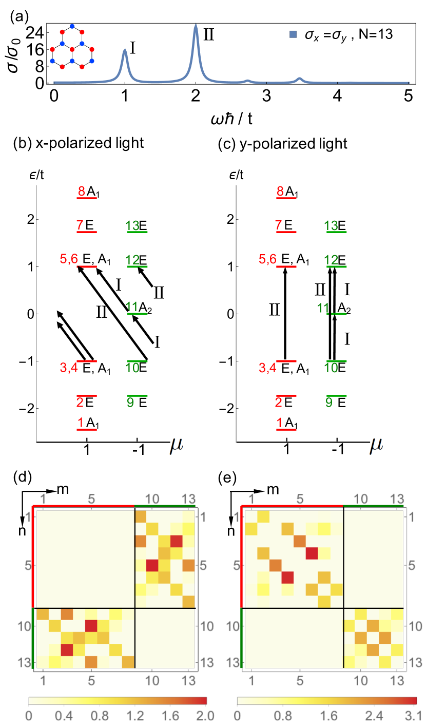
Figure 2: Optical selection rules for the smallest possible triangular graphene quantum dot (GQD) with zigzag edges ($N=13$), in linearly–polarized light. (a) Optical conductivity $\sigma_{\alpha}(\omega)$, showing the equivalence of results for $x$– and $y$–polarized light. (b) and (c) Spectrum of the corresponding tight–binding model [Eq. (16)], in the mirror basis Eq. (38), showing the different allowed transitions for $x$– and $y$–polarized light. (d) and (e) Matrix elements of the corresponding current operators $|\hat{\mathpzc{J}}_{nm}^{x}|^{2}$ and $|\hat{\mathpzc{J}}_{nm}^{y}|^{2}$ [cf. Eq. (24)], in units of $(et/\hbar)^{2}$. Results for $\sigma_{\alpha}(\omega)$ were calculated from Eq. (26), with a Lorentzian of FWHM $2\gamma=0.1\ \text{t}$. Eigenstates are labelled according to their quantum number $n=1\ldots 13$, eigenvalue $\mu_{n}=\pm 1$ [Eq. (38)] and corresponding irrep [cf. Table 1].

Figure 3: Optical selection rules for the smallest possible triangular graphene quantum dot (GQD) with zigzag edges ($N=13$), in circularly–polarized light. (a) Optical conductivity $\sigma_{\alpha}(\omega)$, showing equivalence of results for left– and right–circularly polarized light. (b) and (c) Spectrum of the corresponding tight–binding model Eq. (16), in the rotation basis Eq. (39), showing the different allowed transitions for left– and right–circularly polarized light. (d) and (e) Matrix elements of the corresponding current operators $|\hat{\mathpzc{J}}_{nm}^{L}|^{2}$ and $|\hat{\mathpzc{J}}_{nm}^{R}|^{2}$ [cf. Eq. (24)], in units of $(et/\hbar)^{2}$. Results for $\sigma_{\alpha}(\omega)$ were calculated from Eq. (26), with a Lorentzian of FWHM $2\gamma=0.1\ \text{t}$. Eigenstates are labelled according to their quantum number $n=1\ldots 13$, eigenvalue $\mu_{n}=e^{i\frac{2\pi}{3}\rho_{n}}\;,\;\rho_{n}=0,1,2$ [Eq. (40)] and corresponding irrep [cf. Table 1].

III.1.2 Illustration of optical selection rules for linearly–polarised light

We can make these results more tangible, and somewhat easier to compare with experiments, by examining how optical transitions occur in a specific microscopic model for a GQD with triangular symmetry. The simplest model, which we can consider is the tight–binding model $\hat{\mathpzc{H}}_{0}$ [Eq. 16], as introduced in Section II.2. And in this case, since the system is non–interacting, we can analyze all optical transitions at the level of a single electron.

We first consider results for linearly–polarised light incident on a triangular GQD of the type shown in Fig. 1(a). The optical conductivity $\sigma_{\alpha}(\omega)$ can be calculated using Eq. (26). Results for a triangular GQD containing 13 sites are shown in Fig. 3(a); for purposes of visualisation, $\sigma_{\alpha}(\omega)$ has been convoluted with a Lorentzian of FWHM $2\gamma=0.1\ \text{t}$. For this (very) small GQD, the optical response is dominated by peaks at (I) $\hbar\omega=t$ and (II) $\hbar\omega=2t$. As already noted in Section III.1.1, these results are independent of whether the light is polarised along the x– or y–axis.

In Fig. 3(b) and Fig. 3(c) we show the optical transitions associated with each of these peaks, for the two possible polarisations of light. Eigenstates have been labelled according to their irrep ($A_{1}$, $E$), and further classified according to their eigenvalue under the mirror–symmetry operation

$$\hat{\mathpzc{M}_{y}}|\psi_{n}\rangle=\mu_{n}|\psi_{n}\rangle,\quad\mu_{n}=1,-1\;,$$ (38)

where $\hat{\mathpzc{M}_{y}}$ corresponds to a reflection along the vertical y–axis, as shown in Fig. 1 (a). Each of the peaks in Fig. 3(a) correspond to transitions of a single electron, and it is immediately apparent that all of the associated transitions satisfy the selection rules in Eq. (37). In addition, the fact that $\hat{\mathpzc{J}}^{x}$ ($\hat{\mathpzc{J}}^{y}$) is odd (even) under reflection $\mathpzc{M}_{y}$ imposes the additional condition $\mu_{n}\mu_{m}=-1$ ($\mu_{n}\mu_{m}=1$) on the transitions for $x$–polarised ($y$–polarised) light. However, this additional condition cannot have any effect on the final result for $\sigma_{\alpha}(\omega)$ [Fig. 3(a)], since both components of $\hat{\mathpzc{J}}^{\alpha}$ transform with the same irrep [cf. Table 1, Section III.1.1].

It is also informative to view these transitions in terms of the matrix elements of the current operator $\mathpzc{J}^{\alpha}_{nm}$, expressed now in terms of the single–election eigenstates of $\hat{\mathpzc{H}}_{0}$ [Eq. 16] — cf. Eq. (24). The norm of these matrix elements, $|\hat{\mathpzc{J}}_{nm}^{\alpha}|^{2}$ is plotted in Fig. 3(d) and Fig. 3(e). Once again, states have been labelled according to their eigenvalue $\mu_{n}$ under the reflection $\mathpzc{M}_{y}$. The block off–diagonal form of Fig. 3(d) [block–diagonal form of Fig. 3(e)] therefore reflects the condition $\mu_{n}\mu_{m}=-1$ ($\mu_{n}\mu_{m}=1$). And, while the structure of these matrices looks very different, the final result for $\sigma_{\alpha}(\omega)$ is independent of polarisation, as it must be — cf. Fig. 3(a).

III.1.3 Illustration of optical selection rules for circularly–polarised light

We can also use the example of a non–interacting tight–binding model [Section II.2], to illustrate how the optical selection rules of a triangular GQD function for circularly–polarised light. The main result is easy to anticipate: in the absence of magnetic field, circularly–polarised light can always be decomposed into linear components. And since the optical response of a triangular GQD is independent of the linear polarisation of light, it will also be independent of the circular polarisation of light.

In Fig. 3(a) we show results for the optical conductivity of a triangular GQD with 13 sites, calculated using Eq. (26), for circularly–polarised light. As expected, the result is independent of the (circular) polarisation of the light, and is identical to that found for linearly–polarised light, Fig. 3(a). The optical transitions associated with each of the features in $\sigma_{\alpha}(\omega)$ are set out in Fig. 3(b) (left–polarised light) and Fig. 3(c) (right–polarised light), where eigenstates have been labelled according to their irrep, and classified according to their eigenvalue under the rotation operator

$$\hat{\mathpzc{R}}_{2\pi/3}|\psi_{n}\rangle=\mu_{n}|\psi_{n}\rangle\;,$$ (39)

where

$$\mu_{n}=e^{i\frac{2\pi}{3}\rho_{n}}\;,\;\rho_{n}=0,1,2\;.$$ (40)

Once again, all transitions satisfy the selection rules derived from symmetry, Eq. (37). The transitions for left–polarised light also satisfy the anti–cyclic condition $\rho=\{0\rightarrow 2\rightarrow 1\rightarrow 0\}$, while those for right–polarised light satisfy the cyclic condition $\rho=\{0\rightarrow 1\rightarrow 2\rightarrow 0\}$. Once again, these conditions reflect the way in which the current operator transforms under the rotation $\hat{\mathpzc{R}}_{2\pi/3}$. The same anti–cyclic and cyclic structure is visible in plots of matrix elements, Fig. 3(d) and Fig. 3(e).

Given the role played by rotation symmetry, it is natural to think of the selection rules for circularly–polarised light, in terms of the exchange of angular momentum between a photon and the electrons in a GQD. However this intuition must be approached with a little caution, as $\hat{\mathpzc{R}}_{2\pi/3}$ generates discrete, and not continuous rotations of the dot . None the less, working with eigenstates of $\hat{\mathpzc{R}}_{2\pi/3}$, we find that states with $\rho=1,2$ have a net circulation of current on their bonds, which is to say a net magnetic moment. All of these states transform with the $E$–irrep, and are Kramers doublets, degenerate pairs of states whose current–flow is related by time–reversal symmetry. An example of the current flow within such a Kramers doublet, calculated within a non–interacting tight–binding model is shown in Fig. 14 in Appendix B. Applying a magnetic field lifts the degeneracy of these Kramers doublets — a subject explored in more detail in Ref. Kavousanaki and Dani, 2015.

III.2 Optical selection rules for rectangular graphene quantum dots

In Section III.1, we explored the optical selection rules which arise in the simplest example of a GQD where the planar ($x,y$) components of the current operator transform under the same irrep. We now consider what happens in the simplest example where the planar components of the current operator transform under different irreps — the rectangular GQD shown in Fig. 1(e), with point group, $C_{2v}$. In this case, we will find that the optical selection rules, and associated optical conductivity $\sigma_{\alpha}(\omega)$, does depend on the polarisation of the incident light.

III.2.1 Group–theory Analysis

The symmetry analysis for a rectangular GQD exactly follows the template of Section III.1.1, with one vital difference — we must now work with the representations appropriate to the symmetries of a rectangle, $C_{2v}$, rather than those of a triangle, $C_{3v}$. The representations of the point–group $C_{2v}$ are listed in Table 2. The group $C_{2v}$ comprises the identity ($E$), $\pi$–rotations about the two principal axes in the plane ($C_{2}$), and reflections ($\sigma_{v}$ and $\sigma_{v^{\prime}}$) about the same two axes, as shown in Fig. 1(e). All of these symmetry operations commute, and as a result the group has only one–dimensional irreps : $A_{1},A_{2},B_{1}$ and $B_{2}$. And, crucially, the way in which a polar vector (such as the current operator $\hat{\mathpzc{J}}_{\alpha}$) transforms within $C_{2v}$ is also different from the way in which it transforms in $C_{3v}$. As shown in Table 2, each of the different components of a polar vector transform with different irreps of $C_{2v}$. And, since different polarisations of light couple to different components of $\hat{\mathpzc{J}}_{\alpha}$, this opens the door to a polarisation–dependent optical response.

$C_{2v}$	$E$	$C_{2}(z)$	$\sigma_{v}(xz)$	$\sigma_{v^{\prime}}(yz)$	polar vectors
$A_{1}$	1	1	1	1	z
$A_{2}$	1	1	-1	-1
$B_{1}$	1	-1	1	-1	x
$B_{2}$	1	-1	-1	1	y

Table 2: Character Table of the point–group $C_{2v}$, describing the symmetry of rectangular graphene quantum dots (GQD’s) of the type shown in Fig. 1(e). Eigenstates of a triangular GQD transform with irreducible representations (irreps) $A_{1}$, $A_{2}$, $B_{1}$ and $B_{2}$, while the $x$ and $y$ components of the current operator $\hat{\mathpzc{J}}$ (a polar vector) transform with $B_{1}$ and $B_{2}$ [cf. Weyl, 1950; Heine, 1960; Landau and Lifshitz, 1977; Tinkham, 2003; Wagner, 2001; Jones, 1998]. The corresponding symmetry operations are identity ($E$), $\pi$–rotation about the principal axes ($C_{2}$) and two reflections on symmetry axes ($\sigma_{v}$ and $\sigma_{v^{\prime}}$), as shown in Fig. 1(e).

Once again, we can proceed from the character Table to optical selection rules by applying the general rules for the products of representations Weyl (1950); Heine (1960); Landau and Lifshitz (1977); Tinkham (2003); Wagner (2001); Jones (1998). The two components of the current operator, $\hat{\mathpzc{J}}^{x}$ and $\hat{\mathpzc{J}}^{y}$, transform with $B_{1}$ and $B_{2}$, respectively. And, following the steps of Section III.1.1, the products entering into optical matrix elements can be decomposed as

$B_{1}$	$\times$	$A_{1}$	$\rightarrow B_{1}$   ,		$B_{2}$	$\times$	$A_{1}$	$\rightarrow B_{2}$   ,
$B_{1}$	$\times$	$A_{2}$	$\rightarrow B_{2}$   ,		$B_{2}$	$\times$	$A_{2}$	$\rightarrow B_{1}$   ,
$B_{1}$	$\times$	$B_{1}$	$\rightarrow A_{1}$   ,		$B_{2}$	$\times$	$B_{1}$	$\rightarrow A_{2}$   ,
$B_{1}$	$\times$	$B_{2}$	$\rightarrow A_{2}$   ,		$B_{2}$	$\times$	$B_{2}$	$\rightarrow A_{1}$   .

These results lead to the polarisation–dependent selection rules

$$\sigma_{x}(\omega)\;:\;A_{1}\longleftrightarrow B_{1}\;,\;A_{2}\longleftrightarrow B_{2}\;,$$ (41)

and

$$\sigma_{y}(\omega)\;:\;A_{1}\longleftrightarrow B_{2}\;,\;A_{2}\longleftrightarrow B_{1}\;.$$ (42)

As a direct consequence, in general, for a rectangular GQD,

$$\sigma_{x}(\omega)\neq\sigma_{y}(\omega)\;.$$ (43)

III.2.2 Illustration of optical selection rules for linearly–polarised light

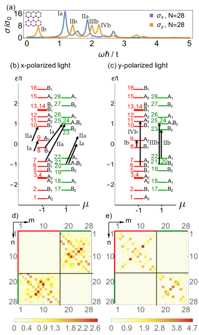
Figure 4: Optical selection rules for a rectangular graphene quantum dot (GQD) of size $N=28$ in linearly–polarized light. (a) Optical conductivity $\sigma_{\alpha}(\omega)$, showing different results for $x$– and $y$–polarized light. (b) and (c) Spectrum of the corresponding tight–binding model Eq. (16), in the mirror basis Eq. (38), showing the different allowed transitions for $x$– and $y$–polarized light. (d) and (e) Matrix elements of the corresponding current operators $|\mathpzc{J}_{nm}^{x}|^{2}$ and $|\mathpzc{J}_{nm}^{y}|^{2}$ [cf. Eq. (24)] in units of $(et/\hbar)^{2}$. Results for $\sigma_{\alpha}(\omega)$ were calculated from Eq. (26), with a Lorentzian of FWHM $2\gamma=0.1\ \text{t}$. Eigenstates are labelled according to their quantum number $n=1\ldots 28$, eigenvalue $\mu=\pm 1$ [Eq. (38)] and corresponding irrep [cf. Table 2].

Once again, it is instructive to illustrate the general, group–theoretical result for the specific example of a rectangular GQD described by the tight–binding model introduced in Section II.2. The corresponding results for the optical conductivity $\sigma_{\alpha}(\omega)$ of a rectangular GQD of size $N=28$ are shown in Fig. 4(a). As expected, results for $x$–polarized light (blue line) are dramatically different from those for $y$–polarized light (orange line), with peaks at different values of $\omega$, labelled I–IV, signalling the different allowed optical transitions. These results are in contrast with the polarisation–independent optical conductivity obtained for a triangular GQD, seen in Fig. 3.

The optical transitions associated with each of these features in $\sigma_{\alpha}(\omega)$ are shown in Fig. 4(b) and Fig. 4(c). Once again, states have been labelled according to their irreps, and further classified according their eigenvalues under the reflection operator $\hat{\mathpzc{M}_{y}}$ [Eq. 38]. The transitions associated with specific peaks in $\sigma_{x}(\omega)$ and $\sigma_{y}(\omega)$ are labelled I–III. All transitions contributing to $\sigma_{x}(\omega)$ satisfy the optical selection rules Eq. 41, while transitions contributing to $\sigma_{y}(\omega)$ satisfy the optical selection rules Eq. 42. The corresponding matrix elements are illustrated in Fig. 3(d) and Fig. 3(e).

III.2.3 Effect of sublattice symmetry–breaking

One of the possibilities discussed in bulk graphene is that interactions could drive a many–electron instability which would spontaneously break the symmetry between the two sites in the unit cell of the honeycomb lattice Kotov et al. (2012). On general grounds, such symmetry breaking is not expected to occur spontaneously in a finite–size system Plischke and Bergersen (2006); Huang (1987). None the less, it is instructive to consider what effect this broken symmetry would have, if it was induced by an external field or perturbation of the graphene structure.

In the case of the rectangular GQD’s considered above, breaking the symmetry between the A– and B–sublattices of sites would reduce the point–group symmetry from C_2v to C₂. Within the group C_2v, the x–component of the current operator $\mathpzc{J}^{\alpha}$ transforms with the irrep B₁, while the y–component transforms with B₂ [cf. Table 2]. As a consequence, the optical conductivity $\sigma_{\alpha}(\omega)$ depends on the polarization $\alpha$ of the incident light [cf. Sec. III.2.1].

In contrast, the group C₂, has only two irreps, A and B, and both the x– and y–components of $\mathpzc{J}^{\alpha}$ transform with the same irrep, B. It follows that, once the symmetry between the A– and B–sublattices is broken, the optical conductivity of rectangular dot is independent of the polarization of the incident light. This is a profound change, and emphasizes the power of optical selection rules in probing the symmetry of a GQD.

III.3 Optical selection rules for GQD’s of other symmetry

In Section III.1 and Section III.2 we have seen how optical selection rules work for a GQD with triangular and rectangular point–group symmetry.

In the case of the triangular GQD, with non–abelian point group $C_{3v}$, the optical conductivity $\sigma_{\alpha}(\omega)$ was found to be polarisation–independent, with $\sigma_{x}(\omega)=\sigma_{y}(\omega)$. This result followed from the fact that both components of the current operator $\hat{\mathpzc{J}}^{\alpha}$ transform with the same two–dimensional irrep, $E$, and therefore transform in the same way under the symmetries of the dot.

In the case of the rectangular GQD, with abelian point group $C_{2v}$, the optical conductivity $\sigma_{\alpha}(\omega)$ was found to be polarisation–dependent, with $\sigma_{x}(\omega)\neq\sigma_{y}(\omega)$. This result followed from the fact that $C_{2v}$ supports only one–dimensional irreps, and the different components of the current operator $\hat{\mathpzc{J}}^{\alpha}$ must therefore transform with different irreps, and so in different ways under the symmetries of the dot.

It might seem counter intuitive that the simpler symmetry structure, $C_{2v}$, should lead to a more complex optical response. However it is precisely the simplicity of the group, with only one–dimensional irreps, which allows the different components of the current operator to transform in different ways. It is the larger and more complex symmetry group $C_{3v}$ which permits both components of the current operator to transform in the same way. And, by the same token, these results generalise straight–forwardly to dots of different symmetry : GQD’s with a point–group such that the x– and y–components of the current operator transform under the same irrep, will show an optical conductivity which is independent of polarisation. Meanwhile, dots with a point–group for which the x– and y–components of the current operator transform under different irreps, will have a polarisation–dependent response. We do not develop this theme further here, but illustrate results for another example, the hexagonal GQD in Appendix A.

IV The role of edge types

		Triangular Zigzag	Triangular Armchair	Hexagonal Zigzag	Hexagonal Armchair	Rectangular
$L$		$\sqrt{3}(N_{h}+1)a$	$3N_{h}a$	$\sqrt{3}(N_{h}-1/3)a$	$(3N_{h}-2)a$	$L_{x}=\sqrt{3}(2N_{h}-1)a$
						$L_{y}=2.5N_{h}a$
$N$		$(N_{h}+1)^{2}+2N_{h}$	$\frac{3}{4}(N_{h}+2)N_{h}$	$6N_{h}^{2}$	$9N_{h}((N_{h}/2)-1)+6$	$2(4N_{h}^{2}-N_{h})$
$N_{0}$		$N_{h}-1$	$0$	$0$	$0$	$0$
$N_{t}$	$N_{h}$ even	$3$	$0$	$3$	$3N_{h}$	$N_{h}$
	$N_{h}$ odd	$3$	$\frac{1}{2}(3N_{h}+1)$	$N_{h}+(-1)^{(N_{h}+1)/2}$	$4N_{h}-3$	$N_{h}+1$

Table 3: Finite–size scaling of degeneracies for different types of regularly–shaped GQD’s, within the tight–binding model, Eq. (16). $L$ is the length of the edge of the GQD, $a$ is the lattice constant, $N_{h}$ the number of hexagons per side, $N$ is the total number of sites, $N_{0}$ the number of zero–energy states, and $N_{t}$ the number of states at energy $\epsilon=t$. For rectangular GQD’s $N_{h}$ refers to the number of hexagons on the side with the armchair edges.

In Section III, we explored the role of symmetry on the optical conductivity, and have shown that the polarization of light can be used to distinguish between dots of different shape.

In this section, we explore the role of edge types in GQD’s by studying the optical conductivity $\sigma_{\alpha}(\omega)$ for triangular, hexagonal and rectangular GQD’s with zigzag and armchair edges and various sizes. Using exact diagonalization of the tight–binding model [Eq. (16)], we show the size evolution of $\sigma_{\alpha}(\omega)$ for dots with a total number of sites up to $N\approx 25,000$ ($\sim 40$ nm) and find features which allow us to separate between dots of zigzag and armchair edges.

Fig. 5 shows an overview of the density of states and optical conductivity for the five different regular–shaped GQD’s considered in this Article (Fig. 1), for sizes up to $N\approx 10,000$ sites. Triangular GQD’s with zigzag edges [Fig. 5(a)] show a peak in the DOS at zero energy for all dot sizes, due to a large number of states localized on the edge that have exactly $\epsilon=0$ within the tight–binding model Ezawa (2007); Zhou and Sheng (2012). The number $N_{0}$ of these “zero–energy” states increases linearly with dot size: $N_{0}=N_{h}-1$Zarenia et al. (2011) [see Table 3], where $N_{h}$ is the number of hexagons per side of the GQD. In the thermodynamic limit the number of edge-states is negligible compared to the total number of states ($N_{0}/N\rightarrow 0$), thus recovering graphene’s zero DOS at $\epsilon=0$.

As seen in Fig. 5(c) and (e), the DOS shows also a feature at zero–energy in hexagonal zigzag and rectangular GQD’s for sizes $N\gtrsim 300$. In fact, for these dots, there are no states with the exact value $\epsilon=0$ (Table 3). However a finite number of states in the vicinity of zero energy approach zero for large dot sizes, resulting in a distinct peak in the DOS. On the other hand, for dots without any zigzag edges [Fig. 5(b) and (d)], the density of states at the chemical potential, $g(\epsilon=0)$ is zero for all sizes.

Graphene’s DOS exhibits two characteristic peaks at $\epsilon=\pm t$ (Van Hove singularities)Castro Neto et al. (2009). Fig. 5 clearly shows that these peaks are recovered for large dots in all shapes and edge types. They are due to the presence of states with energy exactly $\epsilon=\pm t$. For most dots, their number $N_{t}$ scales linearly with dot size (see Table 3). However, unlike the case for zero–energy states, their contribution to the DOS at $\pm t$ does not disappear in the thermodynamic limit. States with energies close to $\pm t$ converge to $\epsilon=\pm t$ in the thermodynamic limit, causing the Van Hove singularities known in graphene. We have found analytical expressions for the wave functions of states with exactly $\epsilon=\pm t$ and will discuss them more detailed in Section V.

Transitions between states of $\epsilon=\pm t$ cause a characteristic peak in the optical conductivity for $\hbar\omega=2t$. The size–evolution shows that the intensity of this peak is shape and edge-type dependent, though particularly pronounced in dots with armchair edges. However, for large enough sizes all GQD’s show an asymmetric Fano resonance–like line-shape, similar to the one in graphene Fano (1961); Mak et al. (2011); Chae et al. (2011).

Interestingly, all GQD’s with at least some zigzag edges, show an additional peak at $\hbar\omega=t$ at least for sizes larger than $N>1000$, because of transitions between zero–energy states and states at $\epsilon=\pm t$. This peak does not appear in the case of dots with purely armchair edges, thus providing a way to differentiate between the two edge types.

Rectangular dots show a different behaviour of the optical conductivity for $x$– and $y$–polarized light [Fig. 5(e)–(f)], as explained in Sec. III.2. When the electric field is in parallel with the zigzag edges ($x$–axis for these dots), the additional peak at $\hbar\omega=t$ shows up. This is due to the fact that the zero–energy states are localised on the zigzag edges, causing a non-zero current. On the other hand, for $y$–polarized light the optical conductivity does not exhibit this feature.

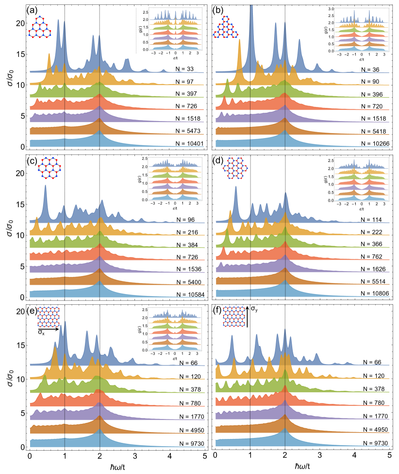
Figure 5: Evolution of the optical conductivity $\sigma_{\alpha}(\omega)$ and density of states $g(\epsilon)$ of the regular–shaped graphene quantum dots (GQD’s) shown in Fig. 1, as a function of the size of the dot. (a) Triangular zigzag, (b) triangular armchair, (c) hexagonal zigzag, (d) hexagonal armchair, and (e)–(f) rectangular GQD for both $x$– and $y$–polarized light. We find that states with $\epsilon=\pm t$ exist in all dots, but are generally more pronounced in dots with armchair edges, causing dominant peaks at $g(\epsilon=\pm t)$. For all dots with zigzag edges, there are states in the vicinity of $\epsilon=0$, causing an additional absorption peak at $\hbar\omega/t=1$. All results were calculated within the tight–binding model Eq. (16), and have been convoluted with a Lorentzian of FWHM $2\gamma=0.1\ \text{t}$ [cf. Eq. (22), Eq. (26)]. For better visualisation each plot has been shifted along the vertical axis.

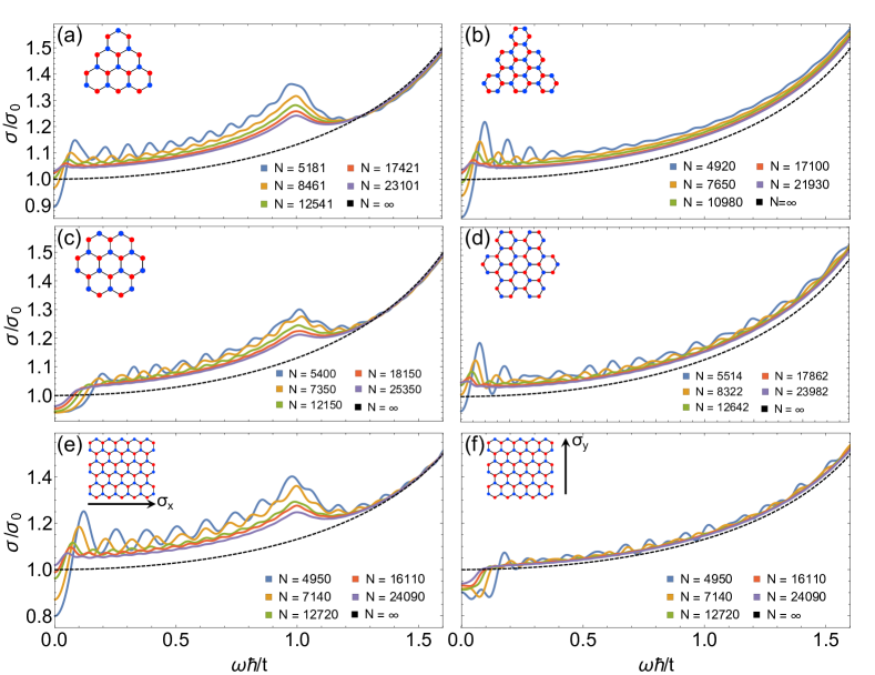
Figure 6: Low frequency part of the optical conductivity $\sigma_{\alpha}(\omega)$ as shown in Fig. 5. (a) Triangular zigzag, (b) triangular armchair, (c) hexagonal zigzag, (d) hexagonal armchair, (e)–(f) rectangular graphene quantum dot for both $x$– and $y$–polarized light, for sizes up to $N\approx 25,000$. The peak at $\hbar\omega/t=1$ in $\sigma_{\alpha}(\omega)$ for dots with zigzag edges (polarization parallel to the zigzag edge) is distinguishable from the featureless conductivity of dots with armchair edges. We compare the results to the analytical solution for a graphene sheet in its thermodynamic limit [see Eq. (28) — dashed line]. All results were calculated within the tight–binding model Eq. (16), and have been convoluted with a Lorentzian of FWHM $2\gamma=0.1\ \text{t}$ [cf. Eq. (26)].

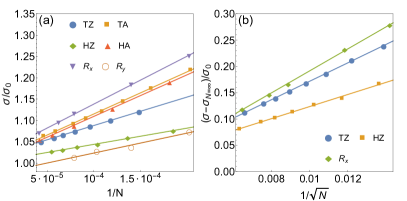
Figure 7: Finite–size scaling of the dominant features in the optical conductivity $\sigma_{\alpha}(\omega)$ from Fig. 6. (a) Linear scaling of the peak maximum for $\hbar\omega/t<0.2$ with the inverse system size $1/N$, showing the trend for all graphene quantum dots (GQD’s) to reach the universal optical conductivity $\sigma_{0}$ [Eq. (2)] in the thermodynamic limit at low frequencies. (b) Scaling of the enhancement in optical conductivity at $\hbar\omega/t=1$, with the linear dimension of the dot $1/\sqrt{N}$, for a dot with zig–zag edges. For $N\to\infty$ we recover the result for bulk graphene, Eq. (28).

To get further insight in the size evolution of the peak at $\hbar\omega=t$, we plot the optical conductivity for dot sizes of $N\approx 5,000-25,000$ ($\approx 20-40$ nm) in Fig. 6 and compare to results of the analytical solution for graphene in its thermodynamic limit [see Eq. (28)].

The right panels of Fig. 6 show, that the optical conductivity for GQD’s with armchair edges converges slowly to the graphene limit, uniformly for all energies. On the other hand, $\sigma_{\alpha}(\omega)$ for dots with zigzag edges has a more complicated behaviour [left panels of Fig. 6]. The peak at $\hbar\omega=t$ is well distinguishable from the background for sizes up to $N\approx 25,000$ ($\sim 40$ nm). For values lower in frequency than this peak, the difference to the graphene limit is larger than in the case of armchair edges. This can be explained by transitions occurring between states of $\epsilon<t$ and states of zero–energy, which are absent in armchair dots. For $\hbar\omega>t$, $\sigma_{\alpha}(\omega)$ coincides with the graphene limit.

As seen in Fig. 6, the plateau of the optical conductivity exhibits strong oscillations. However, in the thermodynamic limit, it approaches the universal conductivity of graphene, $\sigma_{0}$ [Eq. (2)]. This is seen in Fig. 7(a) where the finite–size scaling of the peak at $\hbar\omega/t<0.2$ is shown for all dots under consideration. For all GQD’s, this peak approaches the universal conductivity $\sigma_{0}$ within $2\%$.

In Fig. 7(b) we show the finite–size scaling of the peak at $\hbar\omega/t=1$ for GQD’s with zigzag edges. We find that this peak approaches the value of graphene linearly due to its inverse system length $1/L\sim 1/\sqrt{N}$.

In summary, we discussed the optical conductivity of GQD’s for a variety of shapes, edge types and sizes up to the thermodynamic limit. We showed that polarization along a zigzag edge causes a distinct peak in $\sigma_{\alpha}(\omega)$ at $\hbar\omega=t$. This effect may be used as a way to distinguish between GQD’s with zigzag and armchair edges.

V Localized states with energy $\epsilon/t=\pm 1$

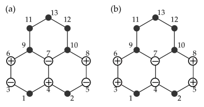
Figure 8: An example of a one–dimensional wave function at energy $\epsilon=\pm t$ in the smallest triangular graphene quantum dot with zigzag edges. (a) Anti-binding ($\epsilon=t$) wave function [see Eq. (45)], (b) binding ($\epsilon=-t$) wave function. Plus (minus) denotes the probability amplitude of $c_{\pm t,i}=+1$ ($c_{\pm t,i}=-1$) of the wave function on site $i$ [as defined in Eq. (44)]. For all other sites we find $c_{\pm t,i}=0$. Such configurations ensure that hopping outside the highlighted sites vanishes.

As discussed in Sec. IV, within the tight–binding model ${\mathcal{H}}_{0}$ [Eq. 16], all GQD’s exhibit states with an exact energy $\epsilon=\pm t$. The number of such states depends on the shape and edge type of the GQD and, in most cases, scales linearly with the dot size (Table 3). In this section we shed light onto the microscopic nature of these states. We present an analytical solution for their wave functions and show that these states exhibit an one–dimensional (1D) character.

The fact that the energy of these states, $\epsilon=\pm t$, coincides with the hopping energy between adjacent sites in the tight–binding Hamiltonian [Eq. (16)], motivates us to seek for wave functions for which electron hopping takes place on single bonds in the honeycomb lattice. Fig. 8 shows an example of such a wave function for a triangular zigzag GQD with energy $\epsilon=t$ (anti–binding) and $\epsilon=-t$ (binding). The wave function $|\psi_{t}\rangle$ is a linear combination of Wannier functions [Eq. (18)],

$$|\psi_{t}\rangle=\sum_{i}c_{t,i}|\phi_{i}\rangle\ ,$$ (44)

where $c_{t,i}$ are appropriately chosen to be $\pm 1$ at the “$+$” and “$-$” sites respectively. In the case of Fig. 8(a), the wave function is explicitly written as

$$|\psi_{t}\rangle\propto-|\phi_{3}\rangle+|\phi_{6}\rangle+|\phi_{4}\rangle-|\phi_{7}\rangle-|\phi_{5}\rangle+|\phi_{8}\rangle\,,$$ (45)

which can be directly shown to satisfy $\hat{\mathpzc{H}}|\psi_{t}\rangle=t~{}|\psi_{t}\rangle$. Eq. (45) has the energy $\epsilon=t$ because electron hopping is non–zero only between pairs of atoms, highlighted in Fig. 8(a). Hopping to, e.g. site 1 is suppressed because of the opposite coefficients on sites 3 and 4. In a similar way, we can construct a binding wave function with $\epsilon=-t$ as seen in Fig. 8(b). We note that these wave functions are 1D–like, since they are non–zero only on pairs of sites along an 1D ladder. This is consistent with their 1D scaling behaviour shown in Table 3.

Figure 9: Examples for one–dimensional wave functions in graphene quantum dots (GQD’s) and bulk graphene. (a) Triangular zigzag, (b) triangular armchair, (c) hexagonal zigzag, (d) hexagonal armchair, (e) rectangular and (f) cluster with periodic boundary conditions (graphene). Boundary conditions set the number and shape of allowed one–dimensional states [see scaling behaviour in Tab. 3], which do not necessarily have to proceed in a straight line, as seen in the first example of (e).

The key for the existence of such states is the presence of a pair of atoms on the edge of the GQD for which each atom has one bond less. This allows the creation of these 1D–ladder states that live on a line of pairs of carbon atoms. Fig. 9 shows 1D wave functions for all GQD’s considered in Sec. IV and for graphene clusters with periodic boundary conditions. It is clear that the number of 1D wave functions depends strongly on the boundary conditions. Therefore hexagonal GQD’s with armchair edges [Fig. 9(d)] favour the presence of these states, which exist for all system sizes [see Table 3].

We should note that these 1D wave functions do not necessarily exist on a straight line, as seen in Fig. 9(b), (c) and (e). In these cases, boundaries allow a bent 1D string of site pairs within the dot, leading to the rather complicated scaling functions of these states in Table 3. Such 1D wave functions also exist in graphene clusters with periodic boundary conditions, as shown in Fig. 9(f).

The one–dimensional character of states at $\epsilon=\pm t$ provides a plausible explanation for the large exciton binding energies of $\sim 500$ meV, found in graphene Yang et al. (2009); Kravets et al. (2010); Mak et al. (2011); Chae et al. (2011); Matković et al. (2012), since confinement in 1D greatly enhances binding. Furthermore, optical resonances in carbon nanotubes are predicted to arise from strongly–correlated 1D excitons Ando (1997). Their binding energies have been predicted with $\sim 400$ meV Wang (2005), comparably close to the results for graphene. A very crude estimate of the local on–site Hubbard $U$ has been done by describing these 1D states with a two–site Hubbard model. Details of this estimate are given in Appendix C.

In summary, we have shown that eigenstates with energy $\epsilon=\pm t$ show a 1D character and can exist in both, GQD’s and graphene. Their 1D nature provides a possible explanation for the unusually high exciton–binding energies found at the M–point in graphene Yang et al. (2009); Kravets et al. (2010); Mak et al. (2011); Chae et al. (2011); Matković et al. (2012).

VI Disorder in a graphene quantum dot : The role of vacancies and asymmetry

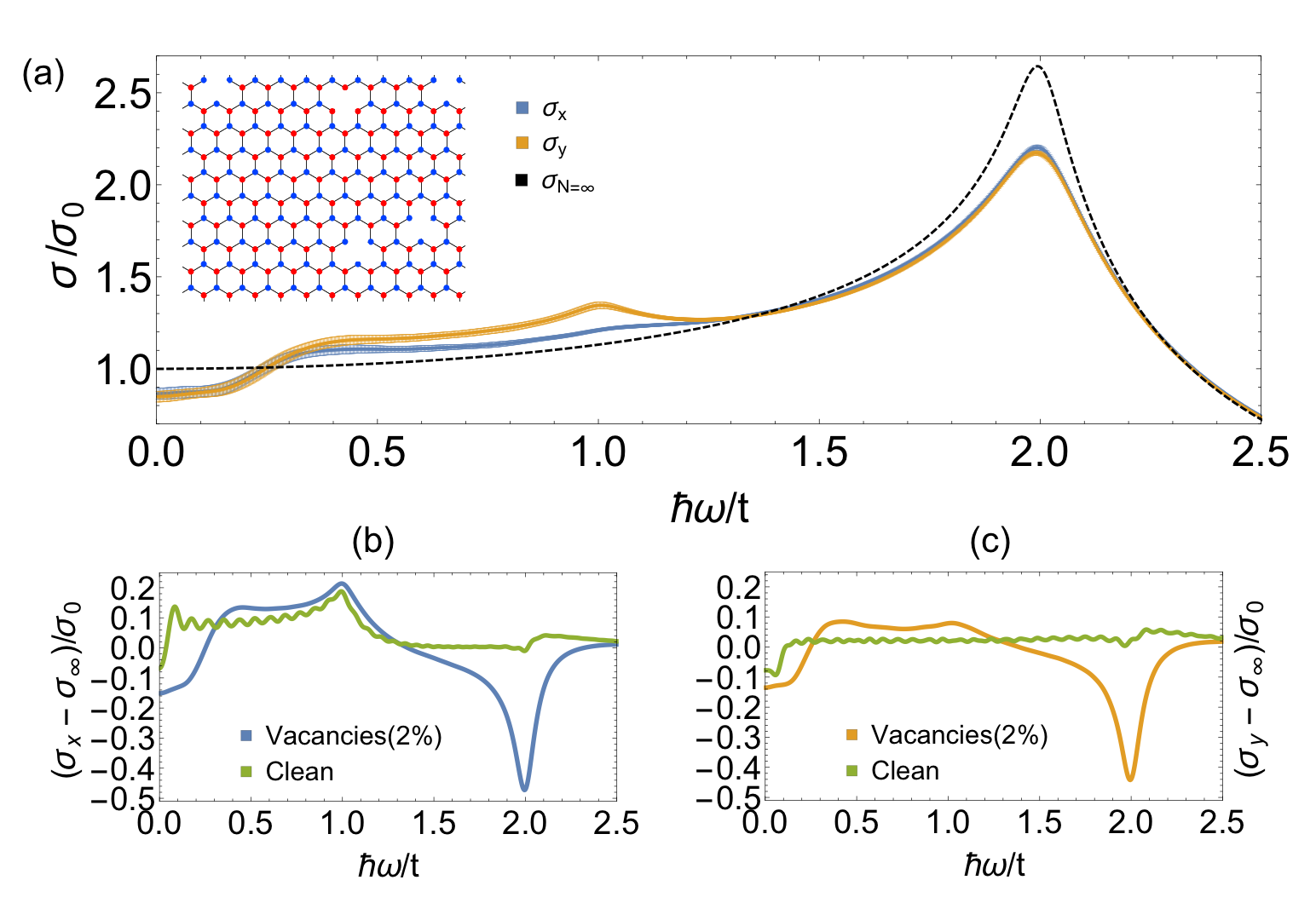
Figure 10: Effect of random site vacancies on the optical conductivity of a rectangular graphene quantum dot (GQD). (a) Optical conductivity of an ensemble of disordered GQD’s, for $x$–polarized (blue curve) and $y$–polarized (yellow curve) light. Error bars show the standard deviation of results with the ensemble, while the dashed line shows equivalent results for an infinite graphene sheet, without vacancies. (b) Difference between optical conductivity of clean and disordered GQD’s and an infinite graphene sheet, for $x$–polarized light. (c) Equivalent results for $y$–polarized light. The disordered GQD shows additional features in the visible spectrum, while the dominant absorption peak at $\hbar\omega/t=2$ is reduced. Results were calculated from Eq. (26), within a tight–binding model for a GQD with $N~{}\approx 10,000$ sites, setting a Lorentzian of FWHM $2\gamma=0.1\ \text{t}$. Disorder–averages were calculated for $2\%$ of randomly introduced vacancies, and averaged over $\approx 100$ realisations.

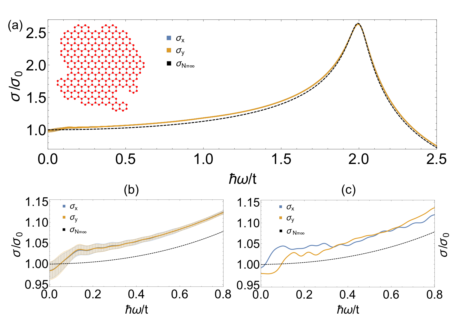
Figure 11: Effect of edge–disorder on the optical conductivity of a graphene quantum dot (GQD). (a) Optical conductivity of an ensemble of disordered GQD’s, for $x$–polarized (blue curve) and $y$–polarized (yellow curve) light. Both curves lay on top of each other. The dashed line shows equivalent results for an infinite graphene sheet, without disorder. (b) Detail of the optical conductivity of disordered GQD’s at low frequencies. Error bars show the standard deviation within the ensemble. (c) Optical conductivity of an individual disordered GQD at low frequencies, showing the difference between $x$– and $y$–polarized light. Results were calculated from Eq. (26), within a tight–binding model for a GQD with $N~{}\approx 10,800$ sites, setting a Lorentzian of FWHM $2\gamma=0.1\ \text{t}$. Disorder–averages were calculated for an ensemble of $\approx 100$ realisations.

Even though GQD’s can be produced in predefined regular shapes Lu et al. (2011); Li et al. (2011); Mohanty et al. (2012); Olle et al. (2012); Yan et al. (2012), techniques like chemical vapour deposition (CVD) or temperature programmed growth (TPG) result in dots with irregular shapesCoraux et al. (2009). Furthermore, surface contamination with adatoms during the fabrication process can introduce scattering potentials, which change the electronic properties of the GQD’s. In the previous sections, we explained how the geometry of GQD’s impacts their optical properties and showed that the presence of zigzag edges results in an additional peak in the optical conductivity at low frequencies. It is therefore useful to examine to which extent these features can survive in the case of irregular shaped dots.

Here we discuss two of such cases: (a) rectangular GQD’s with single atom vacancies, and (b) GQD’s with asymmetric shape. We concentrate on the minimal tight–binding model introduced in Section II.2.

VI.1 The role of vacancies

The role of vacancies on the electronic properties of graphene and its nanostructures has been extensively studied Pereira et al. (2006); Peres et al. (2006); Ostrovsky et al. (2014); Sanyal et al. (2016). Moreover, it has been shown that metallic adatoms on the graphene’s surface — a common source of contamination during fabrication — can be treated theoretically as an atomic vacancy on the graphene lattice in the case of strong local scattering potentials. Yuan et al. (2010)

Here, we discuss the effect of vacancies on the optical conductivity of rectangular GQD’s. As explained in Sec. IV, for clean, vacancy–free dots, optical excitation, polarized along the zigzag edges captures signatures of zero–energy, edge modes in the form of a peak at $\hbar\omega=t$. This peak is absent for polarization along the armchair edges, allowing a distinction between different edge types. We now calculate the optical conductivity for dots with a number of randomly introduced vacancies on the lattice. In our model, we set electron hopping to/from the vacancy sites to zero, which is equivalent to an infinite on–site energy at the vacancies.

Fig. 10(a) shows the optical conductivities $\sigma_{x}(\omega)$ and $\sigma_{y}(\omega)$ for rectangular GQD’s of size $N~{}\approx 10,000$ and $2\%$ vacancies. In comparison with the graphene limit, $\sigma_{N=\infty}(\omega)$ [Eq. (28)], both polarization directions show an enhanced shoulder in the visible region of the spectrum and a decrease of intensity at $\hbar\omega/t=2$.

This is more clearly seen in Fig. 10(b) and (c) where the difference $\sigma(\omega)-\sigma_{N=\infty}(\omega)$ for both clean GQD’s and dots with $2\%$ vacancies is plotted. The dominant peak at $\hbar\omega/t=2$ is significantly reduced by the presence of vacancies. Similarly, for $\hbar\omega/t\approx 1$, the vacancies result in an enhanced shoulder for $\sigma_{y}$, which is absent in the clean GQD. For $\sigma_{x}$, this shoulder is only slightly larger than the one already present for vacancy–free dots.

These features can be explained by the fact that every single vacancy on the graphene lattice creates a zigzag edge around it, which can be seen as an inverse zigzag triangular dot. Therefore additional zero–energy states can be formed along these edges, which allow scattering to the highly degenerate states in the vicinity of the Van Hove singularity and result in the enhanced shoulder in the visible region of the spectrum.

On the other hand, the presence of vacancies destroys some of 1D–wave functions with energy $\epsilon=\pm t$ [see Sec. V]. Consequently, the dominant absorption peak at $\hbar\omega=2t$, which is created by transitions between such states, is reduced.

Our findings are consistent with previous results showing that vacancies in graphene result in the formation of localised states Pereira et al. (2006). Also, calculations in disordered graphene show that it exhibits mid–gap states in the density of states Ugeda et al. (2011, 2010) and an additional peak in the optical conductivity Yuan et al. (2011a).

VI.2 The role of asymmetry

Asymmetry is a certain issue in the fabrication of GQD’s. Techniques like chemical vapour deposition (CVD) and temperature programmed growth (TPG) produce GQD’s of various sizes and shapes Coraux et al. (2009). Even techniques that can create GQD’s with a predefined shape are not free of errors Lu et al. (2011); Li et al. (2011); Mohanty et al. (2012); Olle et al. (2012); Yan et al. (2012).

Here we address this case, by calculating the optical conductivity $\sigma_{\alpha}(\omega)$ for asymmetric dots, showing a random mixture of armchair and zigzag edges.

Fig. 11(a) shows the optical conductivity $\sigma_{\alpha}(\omega)$ for $x$– and $y$–polarized light for asymmetric GQD’s of size $N\approx 10,800$, averaged over $\approx 100$ dots. The mean value of the optical conductivity is very close to the infinite graphene limit, since edge–effects are averaged out. The small offset from the graphene limit is due to finite–size effects.

The effect of averaging is shown more clearly in Figs. 11(b) and (c). Even though on average, $\sigma_{x}$ and $\sigma_{y}$ coincide [Fig. 11(b)], for each individual dot they do not [Fig. 11(c)], due to the absence of symmetry.

VII Conclusions

The discovery of Graphene, more than 10 years ago Novoselov (2004); Novoselov et al. (2005), has sparked a rennaisance in the study of two–dimensional materials, and their potential technological applications Avouris and Dimitrakopoulos (2012); Luo et al. (2013). Graphene quantum dots (GQD’s), offer yet another new opportunity, to control the properties of a graphene sheet by restricting its size and shape Silva et al. (2010); Güçlü et al. (2014). In particular, the ability to control the optical properties of GQD’s has potential applications in fields ranging from quantum computation to solar energyZhu et al. (2011); Jin et al. (2013); Roy et al. (2015); Umrao et al. (2015); Luk et al. (2012); Son et al. (2012); Konstantatos et al. (2012); Zhang et al. (2015); Jiang Wu (2014). However, tailoring the properties of a GQD to a specific application requires the ability to fabricate dots with the desired shape, or to post–select for dots with a given shape after fabrication. In either case, understanding the relationship between the size and shape of the dot and its physical properties is paramount.

In this Article, we have explored the role that size, shape, edge–type and atomic vacancies play in the optical conductivity of GQD’s. Using group theory, we determined the optical selection rules, which follow from the symmetry of a regular–shaped GQD. We find that the optical response is independent of the polarization of the incident light in GQD’s of symmetry, where the in–plane ($x,y$) components of the current operator transform under the same irrep. This has been shown on the example of triangular and hexagonal GQD’s [cf. Fig. 3, Fig. 3]. Meanwhile the optical conductivity is polarization–dependent in GQD’s of symmetry, where the in–plane ($x,y$) components of the current operator transform under different irreps, as shown on the example of rectangular GQD’s [cf. Fig. 4].

We have also explored the optical conductivity $\sigma_{\alpha}(\omega)$ of GQD’s within a simple tight–binding model [Eq. (16)], known to give a good account of the properties of bulk graphene [Castro Neto et al., 2009]. For small GQD’s, $\sigma_{\alpha}(\omega)$ depends strongly on the type of the considered dot, and has many non–universal features [cf. Fig. 5]. These features evolve with size, and the optical response of GQD’s of intermediate size ($N\gtrsim 5,000$ sites, $L\gtrsim 20$nm) has much in common with the response of bulk graphene. In particular this shows a strong peak for UV light, as observed in graphene. None the less, for dots of this size, $\sigma_{\alpha}(\omega)$ still retains tell–tale features which provide important information about edge–geometry of the dot. In particular, we find an additional peak in the optical conductivity at the UV end of the visible spectrum in GQD’s with zigzag edges [cf. Fig. 6].

Within a tight–binding model, both of these peaks in the optical conductivity are intimately connected with the existence of states with energy $\epsilon=\pm t$. We have explored the nature of the wave functions of these states in different–shaped GQD’s, and find that they have a one–dimensional character [cf. Fig. 8 and Fig. 9 ]. Equivalent one–dimensional states also exist for clusters with periodic boundary conditions, where they occur at the M–point in the Brillouin zone [i.e. ${\bf k_{1}}=(\frac{2\pi}{3\sqrt{3}},\frac{2\pi}{3})$ and ${\bf k_{2}}=(\frac{4\pi}{3\sqrt{3}},0)$], and are associated with Van Hove singularities in the single–particle density of states. The one–dimensionality of these wave functions provides a very natural explanation for large binding energies of excitons formed of particles and holes near the M–point Yang et al. (2009); Kravets et al. (2010); Mak et al. (2011); Chae et al. (2011); Matković et al. (2012).

Finally, we discussed the effect of atomic vacancies and shape–asymmetry in the optical response of GQD’s. We showed that atomic vacancies in the lattice enhance the peak in the optical conductivity arising from zigzag edges [cf. Fig. 10]. This is a signature of additional localization around the vacancy sites. In the case of completely asymmetric GQD’s, the optical conductivity is polarization–dependent, although those effects may not be measurable for large distributions of randomly shaped dots [cf. Fig. 11].

An important open question for future studies of the optical properties of GQD’s is the effect of electron–electron interactions. There is already a substantial literature on the effect of interaction in bulk graphene, where the fact that electrons are restricted to two dimensions, and have a Dirac–like dispersion, leads to many departures from conventional Fermi–liquid behaviour Kotov et al. (2012). Given this, it is reasonable to ask how the optical properties of GQD’s might change, if interactions were included ?

The optical selection rules derived in Section III follow from symmetry alone [cf. Section II.1]. For this reason they apply equally to any GQD with a given symmetry, regardless of whether it is described by a simple tight–binding model [Section II.2], or a more general model of interacting electrons which respects the symmetries of the dot. And, while it is possible that interactions could drive changes in the symmetry of an infinite graphene sheet Kotov et al. (2012), such spontaneous symmetry–breaking is not expected in a finite–size GQD Plischke and Bergersen (2006); Huang (1987).

None the less, interactions are known to have a profound effect on electrons on the edges of a graphene sheet Kotov et al. (2012). And, since the optical response of a GQD comprises a discrete set of peaks, even small changes in individual energy levels coming from interactions will be directly visible in $\sigma_{\alpha}(\omega)$. Moreover, the precursors of any bulk symmetry–breaking may also manifest themselves in the spectrum of a finite–size GQD, in much the same way as they do in the finite–size spectra of interacting quantum spin models Bernu et al. (1994). For all of these reasons, we anticipate that interactions will have a significant effect on many of the optical properties of GQD’s.

In small GQD’s, magnetic effects are likely to be important. In this case, interactions can generate local moments at the edges of of a dot Fujita et al. (1996); Fernández-Rossier and Palacios (2007); Feldner et al. (2010); Schmidt and Loss (2010); Luitz et al. (2011); Sasaki and Saito (2008); Kotov et al. (2012); Güçlü and Hawrylak (2013). In addition, interactions will split many of the individual peaks found in non-interacting calculations, where the electrons’ spin plays no role [Section II.2]. The resulting optical conductivity $\sigma_{\alpha}(\omega)$ could, in principle, be calculated from Eq. (10), by writing the interacting Hamiltonian $\hat{\mathpzc{H}}$ as a matrix and diagonalising this numerically. In this way, it is possible to determine both the many–electron eigenstates $|\Psi_{n}\rangle$ [cf. Eq. (9)], and optical matrix elements $\mathpzc{J}^{\alpha}_{nm}$ [cf. Eq. (11)]. Such exact–diagonalisation approaches have already been used to study edge–magnetism in GQD’s and nano–ribbons Feldner et al. (2010); Luitz et al. (2011); Güçlü and Hawrylak (2013). However the exponential growth in the size of the Hilbert space, and the need to determine eigenstates and matrix elements spanning a wide range of energies, will limit exact–diagonalisation studies of $\sigma_{\alpha}(\omega)$ to dots with a very small number of electrons. Moreover, care must always be taken that the current operator $\hat{\mathpzc{J}}^{\alpha}$ [Eq. (11)] is defined in a way which is consistent with the Hamiltonian used Cabib and Kaplan (1973); KUZEMSKY (2011).

In larger GQD’s, where the optical response is a smooth function of frequency, interactions may make themselves felt in more subtle ways. One area where they can have a profound effect is in the renormalisation of energy scales. A prototype for this is provided by the strong peak in the optical response of bulk graphene in the UV spectrum, at $\hbar\omega\sim 4.7$ eV Eberlein et al. (2008); Mak et al. (2011). Within a simple tight–binding model [cf. Eq. (16)] this peak reflects transitions between single–electron states with energy $E\sim\pm t$, and with the usual parameterisation, $t=2.8$ eV [Castro Neto et al., 2009], the peak would be expected to occur for $\hbar\omega=5.6$ eV. However in bulk graphene the particle–hole pairs associated with this peak can be viewed as excitons, and interactions lead to a finite binding–energy, shifting the peak to lower energies  Yang et al. (2009); Kravets et al. (2010); Mak et al. (2011); Chae et al. (2011); Matković et al. (2012). The same should be true for the equivalent, “$2t$” peak in GQD’s of intermediate to large size [cf. Fig. 5], with the added feature that the one–dimensional character of the associated wave functions will enhance correlation effects [cf. Fig. 8]. We also anticipate that interactions will lead to a shift in the peak at $\hbar\omega\sim t$, observed for GQD’s with zigzag edges and/or vacancies [cf. Fig. 6, Fig. 10]. This expectation remains to be verified, but we hope that the results in this Article can provide a useful starting point for future studies.

And for the time being, perhaps the most exciting prospect is the measurement of the optical response of GQD’s in experiment. Given that GQD’s with regular and irregular shapes are now available [cf. e.g. Ref. Yan et al., 2012; Olle et al., 2012], this seems a very real possibility.

Appendix A Optical selection rules for hexagonal dots

A.1 Group–theory Analysis

$C_{6v}$	$E$	$2C_{6}(z)$	$2C_{3}(z)$	$C_{2}(z)$	$3\sigma_{v}$	$3\sigma_{d}$	polar
							vectors
$A_{1}$	1	1	1	1	1	1	z
$A_{2}$	1	1	1	1	-1	-1
$B_{1}$	1	-1	1	-1	1	-1
$B_{2}$	1	-1	1	-1	-1	1
$E_{1}$	2	1	-1	-2	0	0	(x, y)
$E_{2}$	2	-1	-1	2	0	0

Table 4: Character Table of the point–group $C_{6v}$, describing the symmetry of hexagonal graphene quantum dots (GQD’s) of the type shown in Fig. 1(c) and Fig. 1(d). Eigenstates of a hexagonal GQD transform with irreducible representations (irreps) $A_{1}$, $A_{2}$, $B_{1}$, $B_{2}$, $E_{1}$ and $E_{2}$, while the $x$– and $y$–components of the current operator $\hat{\mathpzc{J}}$ (a polar vector) transform with $E_{1}$ [cf. Weyl, 1950; Heine, 1960; Landau and Lifshitz, 1977; Tinkham, 2003; Wagner, 2001; Jones, 1998]. The corresponding symmetry operations are the identity ($E$), $2\times\frac{2\pi}{6}$ ($2C_{6}$), $2\times\frac{2\pi}{3}$ ($2C_{3}$), and one $\pi$–rotation ($C_{2}$) about the principal axes, and 3 reflections on symmetry axes ($\sigma_{v}$ and $\sigma_{d}$), as shown in Fig. 1(c) and (d).

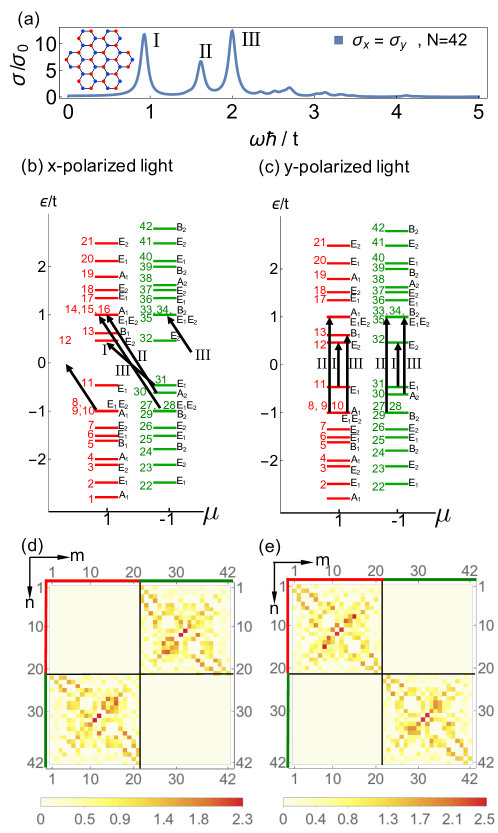
Figure 12: Optical selection rules for the smallest possible hexagonal graphene quantum dot (GQD) with armchair edges ($N=42$), in linearly–polarized light. (a) Optical conductivity $\sigma_{\alpha}(\omega)$, showing the equivalence of results for $x$– and $y$–polarized light. (b) and (c) Spectrum of the corresponding tight–binding model [Eq. (16)], in the mirror basis Eq. (38), showing the different allowed transitions for $x$– and $y$–polarized light. (d) and (e) Matrix elements of the corresponding current operators $|\hat{\mathpzc{J}}_{nm}^{x}|^{2}$ and $|\hat{\mathpzc{J}}_{nm}^{y}|^{2}$ [cf. Eq. (24)], in units of $(et/\hbar)^{2}$. Results for $\sigma_{\alpha}(\omega)$ were calculated from Eq. (26), with a Lorentzian of FWHM $2\gamma=0.1\ \text{t}$. Eigenstates are labelled according to their quantum number $n=1\ldots 42$, eigenvalue $\mu_{n}=\pm 1$ [Eq. (38)] and corresponding irrep [cf. Table 4]

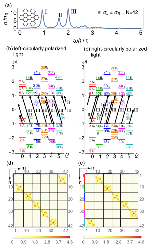
Figure 13: Optical selection rules for the smallest possible hexagonal graphene quantum dot (GQD) with armchair edges ($N=42$), in circularly–polarized light. (a) Optical conductivity $\sigma_{\alpha}(\omega)$, showing equivalence of results for left– and right– circularly polarized light. (b) and (c) Spectrum of the corresponding tight–binding model Eq. (16), in the rotation basis Eq. (39), showing the different allowed transitions for left– and right– circularly polarized light. (d) and (e) Matrix elements of the corresponding current operators $|\hat{\mathpzc{J}}_{nm}^{L}|^{2}$ and $|\hat{\mathpzc{J}}_{nm}^{R}|^{2}$ [cf. Eq. (24)], in units of $(et/\hbar)^{2}$. Results for $\sigma_{\alpha}(\omega)$ were calculated from Eq. (26), with a Lorentzian of FWHM $2\gamma=0.1\ \text{t}$. Eigenstates are labelled according to their quantum number $n=1\ldots 42$, eigenvalue $\mu_{n}=e^{i\frac{2\pi}{6}\rho_{n}}\;,\;\rho_{n}=0,1,2,3,4,5$ [cf. Eq. (40)] and corresponding irrep [Table 4].

In Section III.1, we showed for a triangular GQD, that the optical conductivity is polarization–independent. The given derivation is valid for any GQD where the in–plane ($x,y)$ components of the current operator transform under the same irrep. And this is also the case for the point–group $C_{6v}$ describing an hexagonal GQD.

The symmetry analysis for a hexagonal GQD follows the same concept as shown in Section III.1.1, with the difference, that we must work with point–group symmetries of a hexagon, $C_{6v}$, as listed in Table 4. The group $C_{6v}$ comprises the identity ($E$), $2\times\frac{2\pi}{6}$ ($2C_{6}$), $2\times\frac{2\pi}{3}$ ($2C_{3}$), and one $\pi$–rotation ($C_{2}$) about the principal axes, and 3 reflections on symmetry axes ($\sigma_{v}$ and $\sigma_{d}$), as shown in Fig. 1(c) and (d). Eigenstates of a hexagonal GQD transform with irreducible representations (irreps) $A_{1}$, $A_{2}$, $B_{1}$, $B_{2}$, $E_{1}$ and $E_{2}$, while the $x$– and $y$–components of the current operator $\hat{\mathpzc{J}}$ (a polar vector) transform with $E_{1}$ [cf. Weyl, 1950; Heine, 1960; Landau and Lifshitz, 1977; Tinkham, 2003; Wagner, 2001; Jones, 1998]. As explained for triangular GQD’s, this is the reason for a polarisation–independent optical conductivity $\sigma_{\alpha}(\omega)$.

Following the steps of Section III.1.1, by using the character Table 4, one can resolve the optical selection rules for hexagonal GQD’s by applying the general rules for the products of representations Weyl (1950); Heine (1960); Landau and Lifshitz (1977); Tinkham (2003); Wagner (2001); Jones (1998).

$A_{1}$	$\times$	$E_{1}$	$\rightarrow E_{1}$   ,
$A_{2}$	$\times$	$E_{1}$	$\rightarrow E_{1}$   ,
$B_{1}$	$\times$	$E_{1}$	$\rightarrow E_{2}$   ,
$B_{2}$	$\times$	$E_{1}$	$\rightarrow E_{2}$   ,
$E_{1}$	$\times$	$E_{1}$	$\rightarrow A_{1}+A_{2}+E_{2}$   ,
$E_{2}$	$\times$	$E_{1}$	$\rightarrow B_{1}+B_{2}+E_{1}$   ,

This analysis leads to the optical selection rules

$$A_{1}\longleftrightarrow E_{1}\ ,\quad A_{2}\longleftrightarrow E_{1}\ ,\quad E_{2}\longleftrightarrow E_{1}\ ,$$

$$B_{1}\longleftrightarrow E_{2}\ ,\quad B_{2}\longleftrightarrow E_{2}\ ,\quad E_{1}\longleftrightarrow E_{2}\ ,$$ (46)

which are explicitly independent of polarisation.

A.2 Illustration of optical selection rules for linearly and circularly–polarised light

The optical conductivity $\sigma_{\alpha}(\omega)$ of hexagonal GQD can be calculated explicitly using the non–interacting tight–binding model introduced in Section II.2. The result for linearly–polarised light incident on an hexagonal GQD of size $N=42$ sites is shown in Fig. 12(a). As expected, the result is independent of polarisation, and is dominated by peaks associated at three different values of $\omega$, labelled I—III. The corresponding optical transitions, for x– and y–polarised light, are identified in Fig. 12(b) and Fig. 12(c), where states have been labelled according to their irreps, and further classified according to their eigenvalues under the reflection operator $\hat{\mathpzc{M}_{y}}$ [Eq. 38]. All optical transitions satisfy the selection rules given in Eq. (46). The corresponding matrix elements are illustrated in Fig. 12(d) and (e).

Equivalent results for circularly–polarised light are shown in Fig. 13. The result for $\sigma_{\alpha}(\omega)$, shown in Fig. 13(a) is independent of polarisation, and identical to that found for linearly–polarised light [Fig. 12(a)]. The corresponding optical transitions, for left– and right–polarised light, are shown in Fig. 13(d) and Fig. 13(e), where states have been labelled according to their irreps, and further classified according to their eigenvalues under the rotation operator $\hat{\mathpzc{R}}_{2\pi/6}$ [cf. Eq. 39]. Once again, all transitions satisfy the selection rules given in Eq. (46). The corresponding matrix elements are illustrated in Fig. 13(d) and Fig. 13(e).

From the comparison of these two cases we see clearly that optical selection rules are unaffected by the choice of linearly– or circulary–polarised light, and are independent of polarisation in both cases. This confirms the results of the group theory analysis given in Section A.1.

Appendix B Kramers doublets in triangular graphene quantum dots

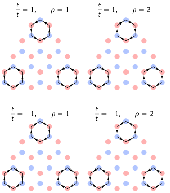
Figure 14: Distribution of the current on bonds within the Kramers–doublet states in triangular graphene quantum dots (GQD’s). By choosing a vector basis of the Hamiltonian Eq. (16), which respects the rotational symmetry of the dot [Eq. (39)], we can distinguish between states of $\rho=1,2$ [see Fig. 3], showing a net circulation of current on their bonds. Hereby, states at $\hbar\omega/t=\pm 1$ show non–zero currents at the edges of the GQD. Results are shown for a GQD with zigzag edges of size $N=33$.

Figure 15: Distribution of the current on bonds within the Kramers–doublet states in hexagonal graphene quantum dots (GQD’s). By choosing a vector basis of the Hamiltonian Eq. (16), which respects the rotational symmetry of the dot [see Eq. (39)], we can distinguish between states of $\rho=1,2,4,5$ [see Fig. 13], showing a net circulation of current on their bonds. Results are shown for a GQD with armchair edges of size $N=42$.

We recognised in Sec. III.1.3 the existence of doubly–degenerate states of Irrep $E$, forming Kramers doublets with time-reversal symmetry. The representation of the Hamiltonian in the basis of the rotational operator gives us access to these states.

In Fig. 14 and Fig. 15 we plot the current (black arrows) within a triangular (N = 33) and hexagonal (N = 42) GQD for energies $\epsilon=\pm t$ for the Kramers doublets. The currents flowing within each member of the Kramers doublet are oriented in opposite directions, such that the two states are connected by time–reversal. An external magnetic field would break this time–reversal symmetry and lift the degeneracy of the Kramers doublets. We would then see changes in the optical absorption spectrum, which can lead to possible manipulations of magnetic moments in GQD’sKavousanaki and Dani (2015).

In Fig. 14 we find currents localised on the tips of the triangle, while in Fig. 15 currents proceed in a circular fashion within the whole dot. We find an absence of currents for states with $\epsilon=0$.

Appendix C Estimate of exciton binding energy within one–dimensional wave functions

Calculations of $\sigma_{\alpha}(\omega)$ within a tight–binding model [Eq. (16)] of an extended graphene sheet show a pronounced peak for $\hbar\omega\sim 2t$ [Stauber et al., 2008; Buividovich and Polikarpov, 2012]. The same is true of a sufficiently large GQD [cf. Fig. 5]. In experiments on graphene sheets, this peak is not observed at $\hbar\omega=2t\approx 5.6\text{eV}$, but at the lower energy of $\hbar\omega=4.6\text{eV}$ [see e.g. Ref. Mak et al., 2011] — a red–shift of $\sim 1$ eV. This shift is usually ascribed to the binding–energy of an exciton formed of particle–hole pairs, due to the interaction between electrons Herbut et al. (2008); Fritz et al. (2008); Yang et al. (2009); Yang (2011a, b); Yuan et al. (2011b).

Building on the insight that electronic states at energy $\epsilon=\pm t$ have a one–dimensional character [cf. Fig. 9, Section V], and are built of two electrons confined to two sites [cf. Fig. 8], we can make a very simple estimate of the exciton binding energy by considering the two–site Hubbard model

$$\hat{\mathpzc{H}}=-t(\hat{\mathpzc{c}}^{\dagger}_{1,\uparrow}\hat{\mathpzc{c}}_{2,\uparrow}+\hat{\mathpzc{c}}^{\dagger}_{2,\uparrow}\hat{\mathpzc{c}}_{1,\uparrow}+\hat{\mathpzc{c}}^{\dagger}_{1,\downarrow}\hat{\mathpzc{c}}_{2,\downarrow}+\hat{\mathpzc{c}}^{\dagger}_{2,\downarrow}\hat{\mathpzc{c}}_{1,\downarrow})\\ +U(\hat{\mathpzc{n}}_{1,\uparrow}\hat{\mathpzc{n}}_{1,\downarrow}+\hat{\mathpzc{n}}_{2,\uparrow}\hat{\mathpzc{n}}_{2,\downarrow})\;.$$ (47)

Diagonalising this Hamiltonian, we find the eigenvalues

$$\epsilon_{0} =\frac{1}{2}\big{(}U-\sqrt{16t^{2}+U^{2}}\big{)}$$ (48)

$$\epsilon_{1} =0$$ (49)

$$\epsilon_{2} =U$$ (50)

$$\epsilon_{3} =\frac{1}{2}\big{(}U+\sqrt{16t^{2}+U^{2}}\big{)}\;.$$ (51)

Optical selection rules allow transitions from the lowest lying energy state with $\epsilon_{0}$ to the intermediate states $\epsilon_{1},\epsilon_{2}$. Since the interaction potential $U$ will lift their degeneracy, low–energy transitions will just occur between $\epsilon_{0}$ and $\epsilon_{1}$, where we find that

$$\Delta\epsilon=\epsilon_{1}-\epsilon_{0}=4.6\ \text{eV}$$ (52)

for

$$U\approx 2.2\ \text{eV}$$ (53)

We note that this is substantially lower than estimates of the on–site potential $U\sim 9.3-10.1\text{eV}$ in the published literature Wehling et al. (2011); Schüler et al. (2013).

References

- Novoselov (2004) K. S. Novoselov, Science 306, 666 (2004).
- Novoselov et al. (2005) K. S. Novoselov, A. K. Geim, S. V. Morozov, D. Jiang, M. I. Katsnelson, I. V. Grigorieva, S. V. Dubonos, and A. A. Firsov, Nature 438, 197 (2005).
- Nair et al. (2008) R. R. Nair, P. Blake, A. N. Grigorenko, K. S. Novoselov, T. J. Booth, T. Stauber, N. M. R. Peres, and A. K. Geim, Science 320, 1308 (2008).
- Ando et al. (2002) T. Ando, Y. Zheng, and H. Suzuura, Journal of the Physical Society of Japan 71, 1318 (2002).
- GUSYNIN et al. (2007) V. P. GUSYNIN, S. G. SHARAPOV, and J. P. CARBOTTE, International Journal of Modern Physics B 21, 4611 (2007).
- Ziegler (2007) K. Ziegler, Phys. Rev. B 75, 233407 (2007).
- Min and MacDonald (2009) H. Min and A. H. MacDonald, Phys Rev Lett 103, 067402 (2009).
- Stauber et al. (2008) T. Stauber, N. M. R. Peres, and A. K. Geim, Phys. Rev. B 78, 085432 (2008).
- Yuan et al. (2011a) S. Yuan, R. Roldán, H. De Raedt, and M. I. Katsnelson, Phys. Rev. B 84, 195418 (2011a).
- Buividovich and Polikarpov (2012) P. V. Buividovich and M. I. Polikarpov, Phys. Rev. B 86, 245117 (2012).
- Geim and Novoselov (2007) A. K. Geim and K. S. Novoselov, Nat Mater 6, 183 (2007).
- Miao et al. (2007) F. Miao, S. Wijeratne, Y. Zhang, U. C. Coskun, W. Bao, and C. N. Lau, Science 317, 1530 (2007).
- Katsnelson (2006) M. I. Katsnelson, The European Physical Journal B 51, 157 (2006).
- Tworzydło et al. (2006) J. Tworzydło, B. Trauzettel, M. Titov, A. Rycerz, and C. W. J. Beenakker, Phys. Rev. Lett. 96, 246802 (2006).
- Ryu et al. (2007) S. Ryu, C. Mudry, A. Furusaki, and A. W. W. Ludwig, Phys. Rev. B 75, 205344 (2007).
- Das Sarma et al. (2011) S. Das Sarma, S. Adam, E. H. Hwang, and E. Rossi, Reviews of Modern Physics 83, 407 (2011).
- Kotov et al. (2012) V. N. Kotov, B. Uchoa, V. M. Pereira, F. Guinea, and A. H. Castro Neto, Reviews of Modern Physics 84, 1067 (2012).
- Silva et al. (2010) A. M. Silva, M. S. Pires, V. N. Freire, E. L. Albuquerque, D. L. Azevedo, and E. W. S. Caetano, The Journal of Physical Chemistry C 114, 17472 (2010).
- Güçlü et al. (2014) A. D. Güçlü, P. Potasz, M. Korkusinski, and P. Hawrylak, Graphene Quantum Dots (Springer Berlin Heidelberg, 2014).
- Güçlü et al. (2010) A. D. Güçlü, P. Potasz, and P. Hawrylak, Phys. Rev. B 82, 155445 (2010).
- Zhu et al. (2011) S. Zhu, J. Zhang, C. Qiao, S. Tang, Y. Li, W. Yuan, B. Li, L. Tian, F. Liu, R. Hu, H. Gao, H. Wei, H. Zhang, H. Sun, and B. Yang, Chemical Communications 47, 6858 (2011).
- Luk et al. (2012) C. M. Luk, L. B. Tang, W. F. Zhang, S. F. Yu, K. S. Teng, and S. P. Lau, Journal of Materials Chemistry 22, 22378 (2012).
- Son et al. (2012) D. I. Son, B. W. Kwon, D. H. Park, W.-S. Seo, Y. Yi, B. Angadi, C.-L. Lee, and W. K. Choi, Nature Nanotechnology 7, 465 (2012).
- Konstantatos et al. (2012) G. Konstantatos, M. Badioli, L. Gaudreau, J. Osmond, M. Bernechea, F. P. G. de Arquer, F. Gatti, and F. H. L. Koppens, Nat Nano 7, 363 (2012).
- Kim et al. (2012) S. Kim, S. W. Hwang, M.-K. Kim, D. Y. Shin, D. H. Shin, C. O. Kim, S. B. Yang, J. H. Park, E. Hwang, S.-H. Choi, G. Ko, S. Sim, C. Sone, H. J. Choi, S. Bae, and B. H. Hong, ACS Nano 6, 8203 (2012).
- Jin et al. (2013) S. H. Jin, D. H. Kim, G. H. Jun, S. H. Hong, and S. Jeon, ACS Nano 7, 1239 (2013).
- Zhang et al. (2015) Q. Zhang, J. Jie, S. Diao, Z. Shao, Q. Zhang, L. Wang, W. Deng, W. Hu, H. Xia, X. Yuan, and S.-T. Lee, ACS Nano 9, 1561 (2015).
- Roy et al. (2015) P. Roy, A. P. Periasamy, C.-Y. Lin, G.-M. Her, W.-J. Chiu, C.-L. Li, C.-L. Shu, C.-C. Huang, C.-T. Liang, and H.-T. Chang, Nanoscale 7, 2504 (2015).
- Umrao et al. (2015) S. Umrao, M.-H. Jang, J.-H. Oh, G. Kim, S. Sahoo, Y.-H. Cho, A. Srivastva, and I.-K. Oh, Carbon 81, 514 (2015).
- Jiang Wu (2014) Z. M. W. Jiang Wu, ed., Quantum Dot Solar Cells, Vol. 15 (Springer New York, 2014).
- Coraux et al. (2009) J. Coraux, A. T. N’Diaye, M. Engler, C. Busse, D. Wall, N. Buckanie, F.-J. M. zu Heringdorf, R. van Gastel, B. Poelsema, and T. Michely, New Journal of Physics 11, 023006 (2009).
- Lu et al. (2011) J. Lu, P. S. E. Yeo, C. K. Gan, P. Wu, and K. P. Loh, Nat Nano 6, 247 (2011).
- Li et al. (2011) X. Li, C. W. Magnuson, A. Venugopal, R. M. Tromp, J. B. Hannon, E. M. Vogel, L. Colombo, and R. S. Ruoff, Journal of the American Chemical Society 133, 2816 (2011).
- Mohanty et al. (2012) N. Mohanty, D. Moore, Z. Xu, T. S. Sreeprasad, A. Nagaraja, A. A. Rodriguez, and V. Berry, Nature Communications 3, 844 (2012).
- Olle et al. (2012) M. Olle, G. Ceballos, D. Serrate, and P. Gambardella, Nano Letters 12, 4431 (2012).
- Yan et al. (2012) Z. Yan, J. Lin, Z. Peng, Z. Sun, Y. Zhu, L. Li, C. Xiang, E. L. Samuel, C. Kittrell, and J. M. Tour, ACS Nano 6, 9110 (2012).
- Müllen (2014) K. Müllen, ACS Nano 8, 6531 (2014).
- Wang et al. (2014) L. Wang, Y. Wang, T. Xu, H. Liao, C. Yao, Y. Liu, Z. Li, Z. Chen, D. Pan, L. Sun, and M. Wu, Nature Communications 5, 5357 (2014).
- Eberlein et al. (2008) T. Eberlein, U. Bangert, R. R. Nair, R. Jones, M. Gass, A. L. Bleloch, K. S. Novoselov, A. Geim, and P. R. Briddon, Phys. Rev. B 77, 233406 (2008).
- Mak et al. (2011) K. F. Mak, J. Shan, and T. F. Heinz, Phys Rev Lett 106, 046401 (2011).
- Castro Neto et al. (2009) A. H. Castro Neto, F. Guinea, N. M. R. Peres, K. S. Novoselov, and A. K. Geim, Reviews of Modern Physics 81, 109 (2009).
- Yang et al. (2009) L. Yang, J. Deslippe, C.-H. Park, M. L. Cohen, and S. G. Louie, Phys. Rev. Lett. 103, 186802 (2009).
- Kravets et al. (2010) V. G. Kravets, A. N. Grigorenko, R. R. Nair, P. Blake, S. Anissimova, K. S. Novoselov, and A. K. Geim, Phys. Rev. B 81, 155413 (2010).
- Chae et al. (2011) D.-H. Chae, T. Utikal, S. Weisenburger, H. Giessen, K. v. Klitzing, M. Lippitz, and J. Smet, Nano Letters 11, 1379 (2011).
- Matković et al. (2012) A. Matković, A. Beltaos, M. Milićević, U. Ralević, B. Vasić, D. Jovanović, and R. Gajić, Journal of Applied Physics 112, 123523 (2012).
- Wallace (1947) P. R. Wallace, Phys. Rev. 71, 622 (1947).
- Fradkin (1986) E. Fradkin, Phys. Rev. B 33, 3257 (1986).
- Lee (1993) P. A. Lee, Phys. Rev. Lett. 71, 1887 (1993).
- Peres (2010) N. M. R. Peres, Reviews of Modern Physics 82, 2673 (2010).
- Zhang et al. (2005) Y. Zhang, Y.-W. Tan, H. L. Stormer, and P. Kim, Nature 438, 201 (2005).
- Gusynin and Sharapov (2005) V. P. Gusynin and S. G. Sharapov, Phys. Rev. Lett. 95, 146801 (2005).
- Shon and Ando (1998) N. H. Shon and T. Ando, Journal of the Physical Society of Japan 67, 2421 (1998).
- Noro et al. (2010) M. Noro, M. Koshino, and T. Ando, Journal of the Physical Society of Japan 79, 094713 (2010).
- Mak et al. (2008) K. F. Mak, M. Y. Sfeir, Y. Wu, C. H. Lui, J. A. Misewich, and T. F. Heinz, Phys. Rev. Lett. 101, 196405 (2008).
- Kuzmenko et al. (2008) A. B. Kuzmenko, E. van Heumen, F. Carbone, and D. van der Marel, Phys Rev Lett 100, 117401 (2008).
- Gogoi et al. (2012) P. K. Gogoi, I. Santoso, S. Saha, S. Wang, A. H. Castro Neto, K. P. Loh, T. Venkatesan, and A. Rusydi, EPL (Europhysics Letters) 99, 67009 (2012).
- Ostrovsky et al. (2006) P. M. Ostrovsky, I. V. Gornyi, and A. D. Mirlin, Phys. Rev. B 74, 235443 (2006).
- Peres et al. (2006) N. M. R. Peres, F. Guinea, and A. H. Castro Neto, Phys. Rev. B 73, 125411 (2006).
- Lee et al. (2011) C. Lee, J. Y. Kim, S. Bae, K. S. Kim, B. H. Hong, and E. J. Choi, Applied Physics Letters 98, 071905 (2011).
- Yuan et al. (2011b) S. Yuan, R. Roldán, and M. I. Katsnelson, Phys. Rev. B 84, 035439 (2011b).
- Yamamoto et al. (2006) T. Yamamoto, T. Noguchi, and K. Watanabe, Phys. Rev. B 74, 121409 (2006).
- Trauzettel et al. (2007) B. Trauzettel, D. V. Bulaev, D. Loss, and G. Burkard, Nat Phys 3, 192 (2007).
- Ritter and Lyding (2009) K. A. Ritter and J. W. Lyding, Nature Materials 8, 235 (2009).
- Hämäläinen et al. (2011) S. K. Hämäläinen, Z. Sun, M. P. Boneschanscher, A. Uppstu, M. Ijäs, A. Harju, D. Vanmaekelbergh, and P. Liljeroth, Phys. Rev. Lett. 107, 236803 (2011).
- Subramaniam et al. (2012) D. Subramaniam, F. Libisch, Y. Li, C. Pauly, V. Geringer, R. Reiter, T. Mashoff, M. Liebmann, J. Burgdörfer, C. Busse, T. Michely, R. Mazzarello, M. Pratzer, and M. Morgenstern, Phys. Rev. Lett. 108, 046801 (2012).
- Jolie et al. (2014) W. Jolie, F. Craes, M. Petrović, N. Atodiresei, V. Caciuc, S. Blügel, M. Kralj, T. Michely, and C. Busse, Phys. Rev. B 89, 155435 (2014).
- Zarenia et al. (2011) M. Zarenia, A. Chaves, G. A. Farias, and F. M. Peeters, Phys. Rev. B 84, 245403 (2011).
- Ezawa (2007) M. Ezawa, Phys. Rev. B 76, 245415 (2007).
- Potasz et al. (2010) P. Potasz, A. D. Güçlü, and P. Hawrylak, Phys. Rev. B 81, 033403 (2010).
- Zhang et al. (2008) Z. Z. Zhang, K. Chang, and F. M. Peeters, Phys. Rev. B 77, 235411 (2008).
- Güçlü et al. (2009) A. D. Güçlü, P. Potasz, O. Voznyy, M. Korkusinski, and P. Hawrylak, Phys. Rev. Lett. 103, 246805 (2009).
- Potasz et al. (2012) P. Potasz, A. D. Güçlü, A. Wójs, and P. Hawrylak, Phys. Rev. B 85, 075431 (2012).
- Güçlü and Hawrylak (2013) A. D. Güçlü and P. Hawrylak, Phys. Rev. B 87, 035425 (2013).
- Yang et al. (2007) L. Yang, M. L. Cohen, and S. G. Louie, Nano Letters 7, 3112 (2007).
- Ozfidan et al. (2014) I. Ozfidan, M. Korkusinski, A. D. Güçlü, J. A. McGuire, and P. Hawrylak, Phys. Rev. B 89, 085310 (2014).
- Akola et al. (2008) J. Akola, H. P. Heiskanen, and M. Manninen, Physical Review B 77, 193410 (2008).
- Heine (1960) V. Heine, Group Theory in Quantum Mechanics (Pergamon Press, 1960).
- Landau and Lifshitz (1977) L. D. Landau and E. M. Lifshitz, Quantum Mechanics: Non-Relativistic Theory, Vol. 3 (Pergamon Press, 1977).
- Tinkham (2003) M. Tinkham, Group Theory and Quantum Mechanics (Dover, 2003).
- Weyl (1950) H. Weyl, The Theory of Groups and Quantum Mechanics (Dover, 1950).
- Wagner (2001) M. Wagner, Gruppentheoretische Methoden in er Physik (Springer, 2001).
- Jones (1998) H. F. Jones, Groups, Representations and Physics (Taylor & Francis, 1998).
- Mahan (2000) G. D. Mahan, Many-Particle Physics, Vol. 15 (Springer US, 2000).
- Cabib and Kaplan (1973) D. Cabib and T. A. Kaplan, physica status solidi (b) 58, 85 (1973).
- KUZEMSKY (2011) A. L. KUZEMSKY, International Journal of Modern Physics B 25, 3071 (2011).
- Plischke and Bergersen (2006) M. Plischke and B. Bergersen, Equilibrium Statistical Physics (3rd Edition) (Wolrd Scientific, 2006).
- Huang (1987) K. Huang, Statistical Mechanics (2nd Edition) (John Wiley & Sons, 1987).
- Goupalov (2009) S. V. Goupalov, Phys. Rev. B 79, 233305 (2009).
- Jungwirth et al. (2016) N. R. Jungwirth, H.-S. Chang, M. Jiang, and G. D. Fuchs, ACS Nano 10, 1210 (2016), pMID: 26607031, http://dx.doi.org/10.1021/acsnano.5b06515 .
- Note (1) Conservation of angular momentum follows from a continuous rotation symmetry, through Noether’s theorem.
- Kavousanaki and Dani (2015) E. G. Kavousanaki and K. M. Dani, Phys. Rev. B 91, 035433 (2015).
- Zhou and Sheng (2012) A. Zhou and W. Sheng, Journal of Applied Physics 112, 094313 (2012).
- Fano (1961) U. Fano, Phys. Rev. 124, 1866 (1961).
- Ando (1997) T. Ando, Journal of the Physical Society of Japan 66, 1066 (1997).
- Wang (2005) F. Wang, Science 308, 838 (2005).
- Pereira et al. (2006) V. M. Pereira, F. Guinea, J. M. B. Lopes dos Santos, N. M. R. Peres, and A. H. Castro Neto, Phys. Rev. Lett. 96, 036801 (2006).
- Ostrovsky et al. (2014) P. M. Ostrovsky, I. V. Protopopov, E. J. König, I. V. Gornyi, A. D. Mirlin, and M. A. Skvortsov, Phys. Rev. Lett. 113, 186803 (2014).
- Sanyal et al. (2016) S. Sanyal, K. Damle, and O. I. Motrunich, Phys. Rev. Lett. 117, 116806 (2016).
- Yuan et al. (2010) S. Yuan, H. De Raedt, and M. I. Katsnelson, Phys. Rev. B 82, 115448 (2010).
- Ugeda et al. (2011) M. M. Ugeda, D. Fernández-Torre, I. Brihuega, P. Pou, A. J. Martínez-Galera, R. Pérez, and J. M. Gómez-Rodríguez, Phys. Rev. Lett. 107, 116803 (2011).
- Ugeda et al. (2010) M. M. Ugeda, I. Brihuega, F. Guinea, and J. M. Gómez-Rodríguez, Phys. Rev. Lett. 104, 096804 (2010).
- Avouris and Dimitrakopoulos (2012) P. Avouris and C. Dimitrakopoulos, Materials Today 15, 86 (2012).
- Luo et al. (2013) X. Luo, T. Qiu, W. Lu, and Z. Ni, Materials Science and Engineering: R: Reports 74, 351 (2013).
- Bernu et al. (1994) B. Bernu, P. Lecheminant, C. Lhuillier, and L. Pierre, Phys. Rev. B 50, 10048 (1994).
- Fujita et al. (1996) M. Fujita, K. Wakabayashi, K. Nakada, and K. Kusakabe, Journal of the Physical Society of Japan 65, 1920 (1996).
- Fernández-Rossier and Palacios (2007) J. Fernández-Rossier and J. J. Palacios, Phys. Rev. Lett. 99, 177204 (2007).
- Feldner et al. (2010) H. Feldner, Z. Y. Meng, A. Honecker, D. Cabra, S. Wessel, and F. F. Assaad, Phys. Rev. B 81, 115416 (2010).
- Schmidt and Loss (2010) M. J. Schmidt and D. Loss, Phys. Rev. B 82, 085422 (2010).
- Luitz et al. (2011) D. J. Luitz, F. F. Assaad, and M. J. Schmidt, Phys. Rev. B 83, 195432 (2011).
- Sasaki and Saito (2008) K. Sasaki and R. Saito, Journal of the Physical Society of Japan 77, 054703 (2008).
- Herbut et al. (2008) I. F. Herbut, V. Juričić, and O. Vafek, Phys. Rev. Lett. 100, 046403 (2008).
- Fritz et al. (2008) L. Fritz, J. Schmalian, M. Müller, and S. Sachdev, Phys. Rev. B 78, 085416 (2008).
- Yang (2011a) L. Yang, Phys. Rev. B 83, 085405 (2011a).
- Yang (2011b) L. Yang, Nano Letters 11, 3844 (2011b).
- Wehling et al. (2011) T. O. Wehling, E. Şaşıoğlu, C. Friedrich, A. I. Lichtenstein, M. I. Katsnelson, and S. Blügel, Phys. Rev. Lett. 106, 236805 (2011).
- Schüler et al. (2013) M. Schüler, M. Rösner, T. O. Wehling, A. I. Lichtenstein, and M. I. Katsnelson, Phys. Rev. Lett. 111, 036601 (2013).