realization of inverse seesaw: neutrino masses, and leptonic non-unitarity
Biswajit Karmakara,111k.biswajit@iitg.ernet.in, Arunansu Sila,222asil@iitg.ernet.in
a Department of Physics, Indian Institute of Technology Guwahati, 781039 Assam, India
Abstract
We provide an based flavor symmetric scenario to accommodate the inverse seesaw mechanism for explaining light neutrino masses and mixing. We find that the lepton mixing, in particular the tri-bimaximal mixing pattern and its deviation through nonzero , is originated solely from the flavor structure of the lepton number violating contribution of the neutral lepton mass matrix. Here we discuss in detail how a nonzero value of is correlated with the other parameters in the framework and its impact on the Dirac CP phase . We also analyze the non-unitarity effects on lepton mixing matrix and its implication in terms of the lepton flavor violating decays, etc.
1 Introduction
Even after the discovery of the Higgs boson at LHC, understanding the origin of smallness associated with neutrino mass still remains an open question. In this respect seesaw mechanism serves as a guiding tool hinting toward the existence of new physics beyond the electroweak scale (). The conventional type-I seesaw [1, 2, 3] tries to explain the smallness of neutrino mass by adding three right-handed (RH) neutrinos to the Standard Model (SM). They have Majorana mass which is representative of the lepton number violation. With the Yukawa couplings of order unity, the left handed neutrinos can be light enough, , provided the new physics scale is sufficiently high GeV or so. Though it suggests an interesting and natural explanation of why neutrinos are so light, such a high new physics scale is beyond the reach of present and future neutrino experiments.
Inverse seesaw [4, 5] on the other hand turns out to be a viable alternate scenario where the new physics scale responsible for neutrino mass generation can be brought down near TeV scale at the expense of involving additional fields (SM singlet fermions ). In presence of additional symmetry like a global , the corresponding neutral lepton mass matrix takes the form
| (1.4) |
using the basis . Note that at this level, neutrinos are massless. Once the lepton number violating term is introduced with , the effective light neutrino mass matrix is given by
| (1.5) |
where . Since the lepton number turns out to be only an approximate symmetry of nature, it is perhaps more natural to be broken by a small amount rather than by a large mass as happened in case of type-I seesaw. Also note that the other mass scale (say the new physics scale) in Eq. (1.4) can be as low as TeV since there exists a double suppression by this new physics scale through Eq.(1.5) and smallness of is then justified to produce correct amount of light neutrino mass.
Apart from the smallness associated with the neutrino mass, the origin of lepton mixing matrix, being quite different from the quark mixing, needs to be understood. The study of underlying principle behind this typical mixing is particularly interesting with the recent finding of nonzero [6, 7, 8, 9]. The present global analysis [10, 11, 12] from several experimental data [13] can be summarized as
, ,
, , .
In this regard, a particular pattern yielding and is called the tri-bimaximal mixing (TBM) [14]. It has received a lot of attention as such a pattern can be elegantly generated using flavor symmetries. Use of non-Abelian discrete symmetries (for a review see [15]) like etc. is very well known [16, 17] in this context. However a deformation from TBM mixing becomes essential after the precise measurement of . The details of such deformation are studied for type-I [18, 19] and type-II seesaw [20] in the context of . In general, extra flavon fields (SM singlet scalar fields transforming non-trivially under the flavor symmetry) are employed333 Deviations from TBM mixing can also be realized by perturbing the vev alignments of the scalars involved [18].. for this approach [21, 22]. Once these fields get their vacuum expectation values (vev), the requisite flavor structure is generated.
In this work we aim to study the lepton mixing matrix in the inverse seesaw framework based on an flavor symmetry. In its minimal form, ref [23] discusses how a TBM pattern can be incorporated in an symmetric inverse seesaw scenario. They have shown (among one of the few possibilities discussed there) that if and matrices all posses the following structure:
| (1.9) |
the light neutrino mass matrix obtains a typical form, [24]
| (1.13) |
The diagonalizing matrix of the above form of is representative of the TBM mixing in the basis where charged lepton mass matrix is diagonal. In [25], authors have shown that in a based inverse seesaw, nonzero can be generated from the correction in the charged lepton sector. Few earlier attempts in realizing inverse seesaw in the framework of discrete flavor symmetries can be found in [26]. Here the construction is such that the charged lepton mass matrix becomes diagonal. Now with a simpler form for and (where and in ), in Eq. (1.5) becomes proportional to identity matrix and hence the structure of matrix coincides with that of . This means that matrix (and hence matrix also) of the form similar to would generate the TBM pattern of lepton mixing matrix. Therefore we finally adopt a matrix different from structure so as to accommodate the observed value of . It is interesting to note that in the inverse seesaw, matrix (the coefficient matrix of the term) being different from zero is the source of violation of the lepton number as stated earlier and now it also turns out that the same is also the source of non-zero as well as other mixings (the charged lepton mass matrix is diagonal) in our scenario. This is a salient feature of our model. We have then discussed the possible correlation between the Dirac CP phase () with and other parameters involved. We have tried to address the smallness associated with the term by considering its origin from a higher dimensional operator. The symmetry along with other non-Abelian discrete symmetries like play important role. We have estimated the effective neutrino mass parameter associated with neutrinoless double beta decay [27, 28] and studied the correlation with as well.
Furthermore being close to , in general the inverse seesaw framework allows non-negligible mixing between the light and heavy neutrino states resulting non-unitarity contributions to the lepton flavor mixing. Since the flavor structure is completely known in our framework, we are then able to study the non-unitarity involved in the set-up and in turn constrain some of the parameters. Lepton flavor violating (LFV) decays also result from this non-unitarity effect. However it turns out in our scenario that branching ratio of those LFV decays are vanishingly small due to exact cancellation of elements involved followed from the particular flavor structure we have considered.
This paper is organized as follows. In the Section 2 below, we describe the construction of the model based on the symmetries of the framework. The detailed phenomenology constraining the parameters of the model from the available data of neutrino experiments takes place in Section 3 and 4. Section 5 is devoted in studying the non-unitarity effect and we comment on lepton flavor violating decays and additional contribution to neutrinoless double beta decay. Finally we conclude in Section 6.
2 The Model
In order to realize the usual inverse seesaw mechanism for the generation of light neutrino masses, we extend he SM particle content by introducing three RH neutrinos, , and three other singlet fermions, as already mentioned. In addition few flavons (, , , , ) are included to understand the flavor structure of the lepton mixing. An additional global symmetry is considered along with the flavor symmetry . The field content of the model and their charges under the symmetry of the model (appropriate for the discussion) are mentioned in Table 1. Once the flavon fields get vev (along suitable directions), the desired structures of the mass matrices are generated as we will find below.
| Fields | ||||||||||||
| 1 | 3 | 1 | 3 | 3 | 3 | 3 | 1 | 1 | ||||
| - | - | - | - | 1 | - | 1 | -1 | 1 | -1 | -1 | ||
| 1 | 1 | 1 | 1 | 1 | 1 | 1 | 1 | 1 | 1 | |||
| -1 | -1 | -1 | -1 | 0 | -1 | 1 | -2 | 0 | -2 | -2 | 0 |
The charged lepton Yukawa terms in the Lagrangian are given by444 In Eq. (2.1), one can introduce a contribution like . But such a term can be absorbed in the original contribution by a mere redefinition of the coupling.,
| (2.1) |
to the leading order, where represents the cut-off scale of the theory and and are the respective coupling constants. Terms within the first parenthesis describe the product of two triplets, which further contracts with singlets , and corresponding to and fields respectively to constitute a true singlet. multiplication rules can be summarized as: , and . Further details about group can be found in [24]. Now we choose the vev of as [17] so that the charged lepton mass matrix turns out to be diagonal in the leading order and can be written as .
The allowed terms in the neutrino sector invariant under the symmetries considered are given by:
| (2.2) |
where are the respective couplings. To construct the flavor structures we consider the flavons acquire vevs along In appendix A, we have written the complete scalar potential invariant under and the additional global symmetry. There we have argued that such choices of vev alignments are indeed possible. With such vev alignment Eq. (2.2) yields the following mass matrix in the basis
| (2.6) |
The mass matrices present in Eq. (2.6) are
| (2.13) |
| (2.20) |
with , and . Note that term follows from a higher dimensional contribution and hence is expected to be naturally small compared to and .
3 Neutrino masses and Mixings
The specific flavor structure of the model ensures that (as evident from Eq. (1.5) and Eq. (2.13)) . Hence in our set-up, the effective light neutrino mass matrix becomes
| (3.1) |
Eq. (3.1) clearly shows that the flavor structure of matrix is entirely dictated by that of . Such an interesting feature was also pointed out in [29], calling it screening mechanism in the context of double seesaw. Additionally we note here that serves the purpose of generating non-zero as well with a modification of its original TBM structure (similar to in Eq. (1.9)). This makes our model an interesting scenario to study, as the source of is connected with the lepton number violating parameter (). Now let us focus our attention to the matrix in Eq. (2.20). It is well known from the very specific structure of the first matrix of right hand side of Eq. (2.20) involving only [17] that it leads to a TBM pattern of the lepton mixing matrix (as the charged lepton mass matrix is diagonal), given by
| (3.5) |
resulting . The second matrix in Eq. (2.20) breaks the TBM pattern and we expect a deviation of from zero. To find out the deviation and possible correlations between the mixing angles and parameters of the model, we first rotate from Eq. (3.1) by so as to get
| (3.6) | |||||
| (3.10) |
As evident, a further rotation by (another unitary matrix) in the 13 plane will diagonalize the light neutrino mass matrix, . The angle and phase associated in are therefore related with the parameters involved in 555The overall factor does not take part in determining the mixing angles and phases. However it would be important in determining the exact magnitude of light neutrino masses as we will see later..
Let us consider the form of as,
| (3.14) |
where and are the angle and phase respectively. The diagonalization of takes place through
| (3.15) |
where are the real and positive eigenvalues and are the phases extracted from the corresponding complex eigenvalues. We are now in a position to evaluate the effective light neutrino mixing such that . The then becomes , where is the Majorana phase matrix with and , one common phase being irrelevant. Now this (charged lepton mass matrix being diagonal) can be compared with which in its standard parametrization is given by [30],
| (3.19) |
where , , the angles , is the CP-violating Dirac phase while and are the two CP-violating Majorana phases.
We consider , and ( they are in general complex) the phases of which are indicated by . For calculational purpose, we define parameters , and the difference of phases by and . As diagonalizes the matrix in Eq. (3.6), and can be expressed in terms of and as,
| (3.20) | |||||
| (3.21) |
Comparing with as in Eq.(3.19), we obtain the following expressions for and Dirac CP phase [20]
| (3.22) |
These correlations are among the usual characteristics of the flavor symmetry [31, 32, 22, 33]. For (depending on the choices of ), the relation implies . Again if , the relation becomes . Hence for both the cases, we have and Eq. (3.21) becomes
| (3.23) |
Using Eq. (3.15), the complex light neutrino mass eigenvalues are evaluated as
| (3.24) | |||||
| (3.25) |
The real and positive mass eigenvalues () can be then extracted having the following expressions,
| (3.26) | |||||
| (3.27) | |||||
| (3.28) |
where and
| (3.29) | |||||
| (3.30) |
The three phases associated with these mass eigenvalues are , where is the overall phase for and are given by
| (3.31) | |||||
Note that the Majorana phases and depend on only.
4 Constraining parameters from neutrino data
Using Eqs.(3.26-3.28) one can define a ratio of solar to the atmospheric mass-squared differences as
| (4.1) |
with and . From the expressions above in Section 3, it is clear that neutrino mixing angle , Dirac CP phase , Majorana phases ( and ) and ratio are functions of four parameters, and . The other two angles () are obtained from the comparison between and . Among these, and ratio are precisely known from the neutrino oscillation data. Since (also the Majorana phases) is yet not be known from the experimental data, we perform the analysis for several choices of . Then the four parameters can be constrained using values of and once we keep one of them fixed. For convenience, we have divided our analysis into five cases: (i) Case A [], (ii) Case B [], (iii) Case C [], (iv) Case D [] and (v) the General Case.
Following [10], the best fit values of eV2 and eV2 along with their 3 ranges are used for our analysis. We have fixed at 0.03. Though there exists another parameter (see Eqs. (3.26-3.28)), this cancels out in the expression for . The magnitude of will be fixed in order to reproduce the solar or atmospheric mass square difference(s). Once this is also obtained, we essentially get the estimate of the absolute neutrino masses and Majorana phases. Expression for the effective neutrino mass parameter appearing in the neutrinoless double beta decay is given by[30],
| (4.2) |
Hence we have a prediction for for the allowed range of parameters. Note that in this analysis we should be able to find out values of and which are consistent with experimental data. However the scales involved as flavons vev, cut-off scale , order of matrix ( the magnitude of ) can not be determined, specifically here in this section. Latter while discussing the non-unitarity effects in Section 5, we would be able to set limits on those scales.
4.1 Case A: []
In this case, we make the simplest choice for the associated phases as . Then Eq. (3.20 and 3.22) can be written as
| (4.3) |
with . Hence we note that solely depends on .
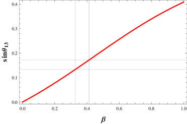
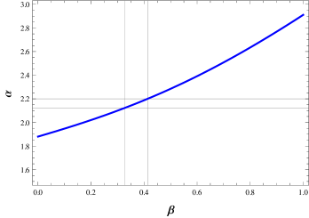
With we get back the TBM pattern of neutrino mixing matrix. In Fig. 1 left panel, we plot the variation of against using Eq. (4.3) the 3 range of (between 0.133 and 0.177 as indicated by the two horizontal lines) predicts a range of : (denoted by the vertical lines).
With , expressions of absolute neutrino masses in Eq. (3.26-3.28) simplify into,
| (4.4) | |||||
| (4.5) | |||||
| (4.6) |
Thereby the ratio of solar to atmospheric mass-squared differences, (as defined in Eq. (4.1)), now takes the form
| (4.7) |
Note that this ratio depends upon both and . To understand this dependence in a better way, we draw the contour plot for [30] in plane as shown in Fig. 1 (right panel). We find that the allowed range of from Fig. 1 (left panel) indicates a range of the other parameter to be within (2.12 - 2.18) as seen from Fig. 1 (right panel). Note that contour plot of provides a one to one correspondence between and values within this range. For example, the best fit values of and corresponds to and . So the sets of values within this allowed range would be used for rest of our analysis in Case A. It is observed that and also fall within their value [10] for the entire allowed range of and .
|
| Parameters/Observables | Allowed Range |
|---|---|
| 0.328-0.412 | |
| 2.12-2.18 | |
| (eV) | - |
| (eV) | 0.102462 - 0.105713 |
| (eV) | 0.0076-0.0085 |
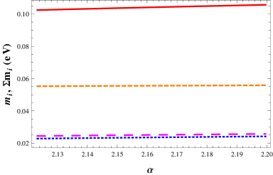
From Eq. (4.4-4.6) it is evident that along with and , individual absolute light neutrino masses depend also upon another parameter . Once we know the sets of that produces in the 3 allowed range and , it is possible to determine from the best fit values of solar (or atmospheric) mass square differences, eV2 ( eV2) [10]. Hence corresponding to a set (), we can determine . Doing so, we find the allowed range for turns out to be eV. Using such a set of values of () we plot the sum of the light neutrino masses and effective mass parameter for neutrinoless double beta decay in the left and right panels of Fig. 2 respectively. Our findings are summarized in Table 2 in terms of allowed ranges for parameters and observables.
4.2 Case B: []
With , Eqs. (3.20) and (3.21) reduce into
| (4.8) |
As before, can be obtained from the relation . Using Eqs.(3.26-3.28), the ratio of solar to atmospheric mass squared differences in this case can be written as
| (4.9) |
where and are same as given in Eqs. (3.30).
|
| (eV) | (eV) | (eV) | |||
|---|---|---|---|---|---|
| 2.162 | 0.372 | 0.0183 | 0.1042 | 0.0222 | |
| 2.155 | 0.393 | 0.0184 | 0.1047 | 0.0225 | |
| 2.136 | 0.448 | 0.0188 | 0.1065 | 0.0233 | |
| 2.103 | 0.521 | 0.0195 | 0.1093 | 0.0245 | |
| 2.060 | 0.596 | 0.0204 | 0.1128 | 0.0260 | |
| 2.011 | 0.666 | 0.0213 | 0.1162 | 0.0274 | |
| 1.965 | 0.728 | 0.0220 | 0.1182 | 0.0280 | |
| 1.928 | 0.782 | 0.0221 | 0.1179 | 0.0275 | |
| 1.901 | 0.827 | 0.0217 | 0.1152 | 0.0259 | |
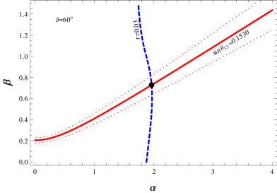
| 1.879 | 0.859 | 0.0210 | 0.1109 | 0.0270 |
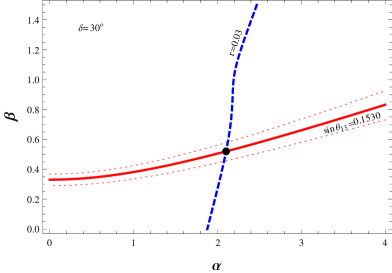
The above expressions show that and both are dependent on three parameters namely and contrary to Case A where they depend only on two parameters and . However if we choose a particular , we can replace dependence in terms of by using the second relation from Eq.(4.8). Then if we draw contours of and in the plane where a simultaneous satisfaction of best fit values of and provide solutions for and with that specific choice of . As an example, we have drawn contour plots for and in Fig. 3 for (left panel) and (right panel) in plane. Intersecting points between the and contours in these plots, denoted by black dots represent the set of solutions () satisfying neutrino oscillation data. and fall in the right range for the entire 3 range of considered. With each such set of solution points () for a fixed , we can compute the other parameter in order to obtain the correct solar (or atmospheric) mass splitting. Here in Table 3 we have provided sets of values for () for various satisfying and obtained from neutrino oscillation experiments.
It is to be noted that with a particular choice of , contour plots for both and are identical with the one obtained from . Here in this set-up, scanning over all values of (with 3 variation of taken into account), sum of the three light neutrino masses and effective mass parameter are predicted to be in the range : and . These are mentioned in the two rightmost columns in Table 3.
4.3 Case C: []
We consider here the other possibility of choosing one of the two phases as zero, . Then we have relations with . This coincides with Eq. (4.3) of Case A. Hence we can use the outcome of Fig. 1 (left panel) for specifying the range of which reproduce the value of (with in 3 allowed range) and respectively. With , the real and positive mass eigenvalues take the form
| (4.10) | |||||
| (4.11) | |||||
| (4.12) |
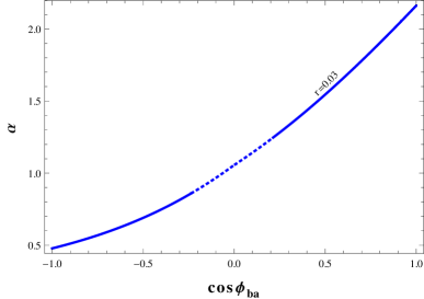 |
In this case, the ratio of solar to atmospheric mass-squared differences , is related to the parameters by the relation,
| (4.13) |
|
The Eq. (4.13) describes a relation between parameters and . We fix at 0.372 which corresponds to the best fit value of as seen from Fig. 1 (left panel). Then and correlation is addressed through a contour plot of in Fig. 4 using Eq. (4.13). We find for , falls with the region . This range is further constrained once we use cosmological constraint on sum of the light neutrino masses to be below 0.23 eV [34]. This exclusion part is indicated by the dotted portion of the contour in Fig. 4. Now in order to have an estimate of absolute neutrino masses, first we need to know the other parameter . Corresponding to the fixed value of , we have sets of values of () which leads to from Fig.4. For each such set of (), we can have the corresponding value in order to get the best fit value for solar mass squared difference, eV2, and obtain
| (4.14) |
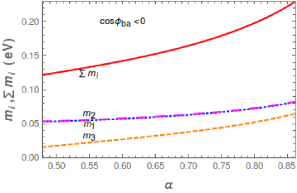
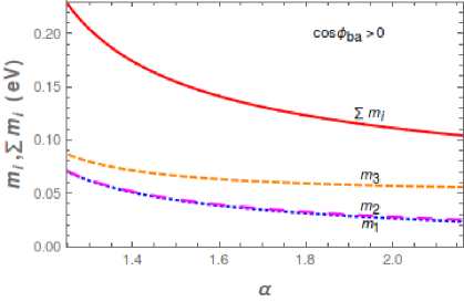
where the Eqs. (4.10, 4.13) are employed and is taken. In Fig. 5 (left panel and right panel) we have plotted absolute neutrino masses () against (with ) where one to one correspondence between and and from Fig. 4 is taken into account. Here and are denoted by blue dotted, magenta large dashed orange dashed and red continuous lines respectively. Note that indicates the inverted hierarchy while corresponds to the normal hierarchy for light neutrinos. We have found the prediction for to be within for normal hierarchy and for inverted hierarchy considering the restricted variation of ( for and for ). Few of our findings are tabulated in Table 4.
| 1.904 | 0.8 | 0.0218 eV | 0.1164 eV | 0.0194 eV |
|---|---|---|---|---|
| 0.814 | -0.3 | 0.0544 eV | 0.0231 eV | 0.0604 eV |
4.4 Case D: []
Now, if we consider , then Eqs. 3.20 and 3.21 can be written as
| (4.15) |
and hence again can be computed using the relation . The real and positive mass eigenvalues now take the form
with
| (4.16) | |||||
| (4.17) |
Using above expressions for light neutrino masses we can write the ratio of solar to atmospheric mass squared difference as
| (4.18) |
Clearly just like Case B, here also both and both depends on and the common phase . Following the same prescription as in Case B, one can draw contours for best fit values of and in the plane. Intersecting points of these two contours then represent simultaneous solutions for both and for a particular value of . In Fig. 6 we have drawn such contours for (left panel) and (right panel) for demonstrative purpose. In this plot, black dots represent the intersecting points for and contours and hence the solutions for and . Here we find that solutions satisfying neutrino oscillation data exist for all values of between and as given in Table 5. We find that the contour plots for both and with a specific value coincides (and hence the solutions for , ) with the one with other values (in the range 0 to ) obtained from .
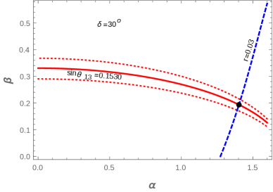 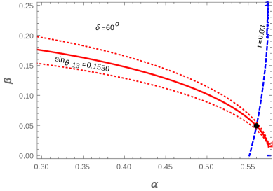
|
| (eV) | (eV) | (eV) | |||
|---|---|---|---|---|---|
| 2.162 | 0.372 | 0.0183 | 0.1042 | 0.0220 | |
| 2.039 | 0.343 | 0.0194 | 0.1057 | 0.0221 | |
| 1.755 | 0.272 | 0.0223 | 0.1095 | 0.0214 | |
| 1.403 | 0.194 | 0.0273 | 0.1187 | 0.0225 | |
| 1.070 | 0.131 | 0.0354 | 0.1365 | 0.0319 | |
| 0.792 | 0.084 | 0.0472 | 0.1659 | 0.0447 | |
| 0.560 | 0.049 | 0.0658 | 0.2159 | 0.0641 | |
| 0.518 | 0.043 | 0.0701 | 0.2301 | 0.0694 | |
| 0.359 | 0.023 | 0.1011 | 0.3157 | 0.1000 | |
| 0.175 | 0.006 | 0.2027 | 0.6144 | 0.2022 |
Following the same algorithm as described in Case B, in the last two column of Table 5 we have listed allowed values for sum of all three light neutrinos and effective mass parameter. Therefore varying between to , we find range of few quantities as and respectively. Therefore imposing the constraint eV on sum of all three light neutrinos coming from Planck [34], the allowed range for gets restricted and it finally lies in the range (in terms of the full range , other allowed ranges are and , ). In this case only the normal hierarchy results as in Case A and B.
4.5 General Case
In the previous sub-sections, we have considered four different cases with specific choices for and/or for our analysis on neutrino masses and mixing. Here we discuss the most general case where we allow the variation of and for their entire range between 0 and . For this purpose, we employ Eqs. (3.20-3.22) in order to analyze the mixing angles. On the other hand, the ratio of solar to the atmospheric mass-squared differences , defined in Eq. (4.1), can also be computed once we use the general expressions for absolute neutrino masses given in Eq. (3.26-3.28).
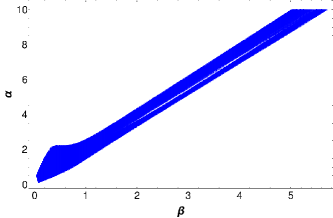 |
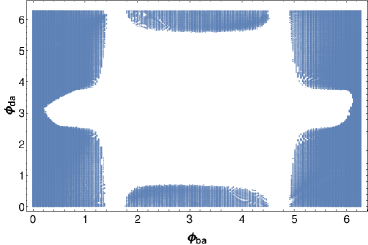
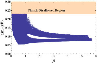
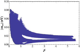
Now using the allowed ranges for and [10], we represent the allowed regions for and in Fig. 7 represented by the blue patch. Here and are allowed to vary within their full range ( to ). However it turns out that only a portion of this entire range can actually satisfy the required and through Eqs. (3.20-3.22) along with the range of depicted in Fig. 7. This is shown in Fig. 8 in the plane.
 |
Knowing the allowed range of and their correlation with phases , we plot in Fig. 9 the prediction of the model in terms of sum of the three light neutrino masses () in the left panel and effective mass parameter for neutrinoless double beta decay () in the right panel as functions of . In the left panel of Fig. 9, the horizontal orange patch represents the excluded region by the upper bound on sum of the absolute neutrino masses eV, whereas in the right panel of the same figure we have already included this additional constraint to plot .
|
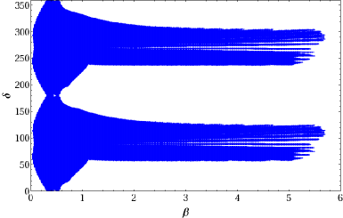
Finally in Fig. 10, we show the allowed range of the Dirac CP phase against the range of (allowed) where we consider simultaneously the corresponding allowed range of and following Figs. 7-9.
 |
5 Non-unitary effect
In Section 3, we have determined the neutrino mixing matrix and identify it with the (charged lepton mass matrix being diagonal) as it diagonalizes the effective light neutrino mass matrix through the unitary transformation . However the should receive a correction over as the heavy states carries an admixture with the light neutrinos [35]. To clarify, suppose is the diagonalizing matrix which makes into the block diagonal form first,
| (5.3) |
At this point the light neutrino mass matrix and the other one is given by
| (5.6) |
in the lowest order [36]. Let be the matrix of the form
| (5.9) |
which will do the individual diagonalization, and are expected to diagonalize and respectively (remember that is the diagonalizing matrix of as already discussed in Section 3). So finally diagonalizes the entire matrix such that . One can decompose as follows:
| (5.12) |
where the block is the leading order replacement of matrix which is non-unitary [37, 38]. It is shown [37, 40] that , where the non unitary effect is parametrized by
| (5.13) |
with as defined before. The present bound on (at 90 C.L.) can be summarized as [39]
| (5.17) |
In our case is proportional to identity as mentioned before and so as . In the present framework turns out to satisfy say, and hence the above bound on can be translated into
| (5.18) |
where . Using this bound, we can now estimate the scales involved in our scenario, etc. For simplicity we assume all the flavons have the same vevs . Then is given by where . Hence the common flavon vev is bounded by
| (5.19) |
which follows from Eq.(5.18).
5.1 Determining the scales () involved in the set-up
Note that the parameter defined in Section 3 can be written as
| (5.20) |
once the common flavon vev is assumed and is inserted. As we already have an estimate for the range of for all cases (A, B, C and D), we can use that input on to study the correlation between and for various choices of while is fixed, say at unity. This correction however satisfy Eq. (5.19) and we discuss it below case by case.
5.1.1 Case A: []
In this case, we have found eV corresponding to the set of parameters () which produces the best fit value of and so as to have the solar and atmospheric mass squared splittings eV2 and eV2 respectively via Eqs. (4.4-4.6).
 |
| in GeV (for ) | |||
|---|---|---|---|
| in GeV (for ) |
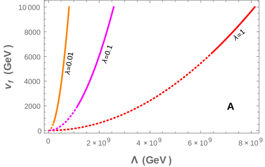
Now using this particular value of , we employ Eq.(5.20) to have an estimate of and once the couplings and are fixed. In Fig. 11, we plot the contour lines for eV in the plane for different choices of . Here is assumed to be unity for simplicity. Following Eq. (5.19), the correlation gets further constrained. Depending on the specific choices of , the lower bound on is obtained through Eq. (5.19). The portion of each contour line which does not satisfy Eq.(5.19) is indicated by the dotted segment. Note that corresponding to a specific choice of the non-unitarity parameter , would fixed through (for fixed ) which then indicates a particular . In Table 6, we provide some such specific choices of corresponding to different choice of . We find that with small enough, the cut-off scale can also be lowered TeV.
5.1.2 Case B: []
|
| in GeV | ||||||
| in GeV | ||||||
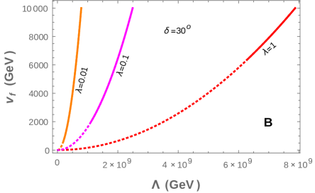
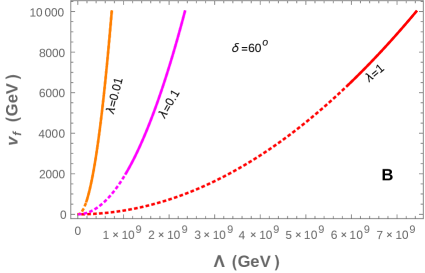
In Section 4 we have seen that for , and depend not only on , but also on the choice of Dirac CP phase . We have already listed our finding toward this dependency in Table 3. Corresponding to each , we have sets of and from Table 3. Now for a fixed and we can study the correlation of and in a similar way as described in Case A above. In Fig. 12, we have studied this correlation for two different choices for , eV (left panel) and , eV (right panel). We consider and choices for (orange line), 0.1 (magenta line) and 1 (red line) in both panels are shown. Since (see Table 3) does not change much with the change of , correlation between and remains almost unaltered as seen from the two panels of Fig. 12. The dotted section of each contour line in Fig. 12 represents the excluded part in view of Eq. (5.19). With some specific choices of (satisfying Eq. (5.18)) we have listed the corresponding scale in Table 7.
5.1.3 Case C: []
|
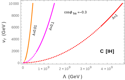
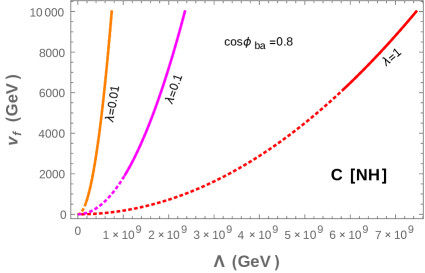
In this case, as we conclude from Fig. 4, the range of is restricted as for and for . We have found that represents inverted hierarchy while stands for normal hierarchy. Here turns out to be zero. Therefore for a specific value of (and hence also for ) we obtain the corresponding value of as mentioned in Table 4. Using that particular , we draw contour plot of in - plane in Fig. 13 where Eq. (5.20) is employed. Left panel of Fig. 13 is for inverted hierarchy of light neutrinos and right panel represents the case of normal hierarchy. Using the non-unitarity constraints through Eq. (5.19), similar to Case A and Case B, here also we indicate the disallowed portion of - correlation. Considering some specific choice of , we provide sample values of in Table 8.
| in GeV | ||||||
| in GeV | ||||||
5.1.4 Case D: []
With the consideration , we have already discussed in the previous section that and are correlated with the choice of . We have listed as well as for different allowed values of in Table 5. As discussed before, here also we can plot the dependency of using Eq. (5.20) and estimate the allowed regions for and employing Eq. (5.19). In Fig. 14 we have plotted this dependency for various choice of with (left panel) and (right panel). In both of these panels orange, magenta and red lines stand for and 1 respectively. Following this we have listed few representative values of in Table 9.
| in GeV | ||||||
| in GeV | ||||||
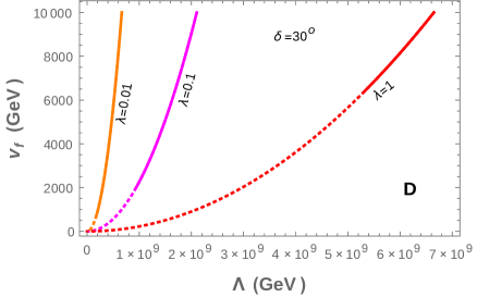 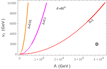
|
5.1.5 General Case
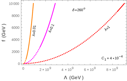
From our previous analysis in section 4, we choose a particular value of for this general case (a value close to recent hint [9, 10, 11, 12]) to study the scales . The set of parameters that would correspond to this value of are found to be and which satisfy constrains imposed from mixing angles, and eV. Here is found to be 0.0147 eV in order to have adequate solar and atmospheric splittings. Using this through Eq. (5.20), we then obtain the contour plot of against as shown in Fig. 15 for different choices of . The dotted portion in each curve indicates the excluded part in view of Eq. (5.19) with (left panel) and (right panel). These numerical estimates are summarized in Table 10.
| in GeV (for ) | |||
|---|---|---|---|
| in GeV (for ) |
|
5.2 Lepton flavor violation
In view of the presence of this non-unitarity effect, the neutrino states ( with ) appearing in the SM charged current interaction Lagrangian now can be written as,
| (5.21) |
where the matrix (see Eq. (5.12)) is conventionally denoted by . and are the light and heavy neutrino mass eigenstates respectively. Then in a basis where charged leptons are diagonal (as in our case), the charged current interactions have contributions involving three light neutrinos and six heavy neutrinos as
| (5.22) |
These nine neutrino states can therefore mediate lepton flavor violating decays like in one loop ( ). Resulting branching ratio for such processes ( in the limit ) now can be written as [42, 43, 45, 46, 47, 48, 49, 50, 51],
| (5.23) |
where
| (5.24) |
Here , with as the weak coupling, is electroweak mixing angle, is boson mass and is the total decay width of the decaying charged lepton . Current upper bound for the branching ratio of the LFV decays are [30] (at 90% CL)
| (5.25) | |||||
| (5.26) | |||||
| (5.27) |
Another important lepton flavor violating decay is also worthy to mention and details of computation of branching ratio calculation can be found in [42, 43]. Current upper limit for this decay is ( CL) [30].
Since the flavor structure of the neutrino mass matrix is already fixed in our present scenario (from the and additional symmetry consideration), it would provide some concrete understanding for the LFV processes in this inverse seesaw model. Both the and matrices play the instrumental role here. Remember that, is the diagonalizing matrix for the light neutrinos, defined by as discussed in section 3. Hence this can be obtained in terms of and . The non-unitary parmeter is required to satisfy, as discussed earlier. Therefore we can completely evaluate , once a specific value of is chosen.
where is the diagonalizing matrix of given in Eq. (5.6). As previously mentioned, in our scenario is proportional to identity matrix of order , . Hence, the matrix turns out to be
| (5.29) |
Using Eqs. (2.13) and (2.20), we find
| (5.33) |
where we have used the explicit flavor structure of and .
We now proceed to find out the form of , the diagonalizing matrix of . Note that the matrix can first be block diagonalized by as
| (5.36) |
where is given by (in our scenario both and are symmetric matrices)
| (5.39) |
Here we have neglected the terms involving higher orders in as expected in inverse seesaw scenario in general. Now the upper and lower block matrices of carry the form of matrix itself (or ). The presence of just redefines the previous parameter by (see Eq. (2.13) and (2.20)). Therefore we can follow the similar prescription for diagonalizing these blocks as we did in case of diagonalization. Hence can further be diagonalized by with
| (5.42) |
where has the form similar to ,
| (5.46) |
Therefore the diagonalizing matrix of can be written as
| (5.51) |
In order to find , we use as obtained in Eq. (5.33). Furthermore, we get and appearing in as discussed earlier. Hence following the same way as in Eq. (3.20) and Eq. (3.21) we find
| (5.52) | |||||
| (5.53) |
with and we use the definition of and as,
| (5.54) |
For simplicity we discard phase difference between and , and set .
Note that from our understanding in Sections 3-4, we can have estimates over the parameters along with the phases in order to satisfy , other mixing angles, , individual solar and atmospheric splittings, also to be consistent with the upper bound on sum of the light neutrino masses. Specific choice of enables us to compute magnitude of the flavon vev and hence from Eq. (5.20). With all these values in hand we can finally evaluate parameters and appearing in . Here we consider 666A common phase as described in the discussion above Eq. (3) in Section 3, is irrelevant for neutrino phenomenology and hence we put it at zero. We also set phases of and to zero. . Now following the analytic expressions in Eqs. (5.28-5.33), (5.42-5.54), we can estimate and and hence the corresponding contribution to the branching ratio (see Eq. (5.23)). Due to particular flavor structures of the matrices as well as and , we find and are such that this scenario predicts vanishingly small branching ratio () for LFV decays.
In addition, we have performed the evaluation numerically also. In order to evaluate it, we need to diagonalize the entire neutrino mass matrix . Since the neutrino mixings are entirely dictated by the flavor structure of matrix, we could have find the entire numerically with the choices of along with the phases as done in cases A, B, C, D and the general case. However to compute and , we need consider to and separately (for example, to have , we assume ). Then following Eq. (2.6), we can entirely construct the matrix numerically. Then with the help of Mathematica777We also use Takagi factorization [44] to find ., we are able to find the diagonalizing matrix (and hence matrix also) and have estimate over the LFV decays. It turns out that the numerical estimate coinsides with our analytical evaluation of vanishingly small branching ratios for LFV decays to a good extent.
5.3 Neutrinoless double beta decay and contribution of heavy neutrinos
We note that in addition to the standard contribution to the effective mass parameter involved in neutrinoless double beta decay as described in Section 3, there will be additional contribution due the presence of mixing between light and heavy neutrinos ( with nonzero ). Hence the half life associated with neutrinoless double beta can be expressed as [54, 55, 57, 58]
| (5.55) |
where is the phase space factor and MeV [54]. Here is the mass of electron, is the mass of proton, is the nuclear matrix element for light neutrino states and is nuclear matrix element for heavy neutrino states. Here the first and second contribution in Eq. (5.55) is due to the light and heavy neutrinos respectively. We already have an estimate for the first contribution (with ) as provided in several tables of Section 4, which turns out to be of order eV. Now with some specific choice of and , we can determine the matrix numerically as discussed in the previous subsection where information on other parameters are taken from Section 4 (different cases). Then we evaluate numerically the . In order to maximize this contribution, we consider lowest value of which is allowed from Eq. (5.19). It turns out then that the second contribution remains sub-dominant ( eV or less) compared to the first contribution of Eq. (5.55). The smallness of the second term can also be understood from our finding for as . A naive estimate for this contribution (to ) therefore is of order . The using the lowest possible consistent with Eq. (5.19), the estimate indicates that this contribution is essentially small compared to the first contribution. So the effective mass involved in the neutrinoless double beta decay process is mostly unaffected with the presence of heavy neutrinos in the present set-up.
6 Conclusion
We have considered an inverse seesaw framework embedded in a flavor symmetric environment in order to study whether it can accommodate the neutrino masses and mixing as suggested from present experimental data, particularly in view of nonzero . We employ an discrete symmetry which is concocted with a global symmetry. We note that the flavor structure of light neutrino mass matrix is essentially dictated by that of the matrix itself, which is the matrix containing the lepton number breaking contribution in the inverse seesaw scenario. The flavor structure of matrix is generated when the flavons have vevs. We notice that the typical structure of this matrix can lead to a lepton mixing consistent with neutrino data where the charged lepton mass matrix is found to be diagonal in the framework. In doing this analysis, we have studied the correlation between different parameters of the model and their dependence on the neutrino parameters such as mass-squared differences, mixing angles etc., evaluated from experimental results. Dependency on the Dirac CP violating phase is also studied.
Since there exists a small mixing between light and heavy neutrino states in the framework, we have also checked the non-unitarity effects in our set-up which contribute to LFV processes, neutrinoless double beta decay etc.. We have found that owing to the typical flavor structure of the neutrino mass matrix here, the effective contribution of it to the LFV processes and neutrinoless double beta decays are vanishingly small. It can be noted that the matrix results from the breaking of a flavon which carries charge under the global . Hence we expect to have Goldstone boson or majoron () [56]. It may open Higgs boson decay channel () and demands extensive analysis in the context of current and future LHC data. Discussions in this direction can be found in [52, 53]. Particularly current 13 TeV run of LHC will be important for such analysis. However further discussion in this regard is beyond the scope of the present study. Since the new physics scale in the present set-up is around few TeV, collider aspects of such a scenario turns out to be intersting and discussion in this direction can be found in [59, 60].
Appendix
Appendix A VEV alignments of flavons
The most general renormalizable potential involving all the flavons of our set-up which is invariant under and respecting can be written as
where
| (A.1) | |||||
| (A.2) | |||||
| (A.3) | |||||
| (A.4) | |||||
| (A.5) | |||||
| (A.6) | |||||
| (A.7) | |||||
| (A.8) |
Here the explicit multiplication of are taken into account. In general this potential involves several free parameters. These plenty free parameters should naturally allow therefore the required vev alignment of the flavons we considered, . For example, with a particular choice like the followings888Along the specified vev directions, terms involving the couplings , , , , , , , , , , ,, , , , , , , , , , , , , and do not contribute.
can actually lead to a common vev 1 TeV along the required direction.
References
- [1] P. Minkowski, Phys. Lett. B 67, 421 (1977).
- [2] M. Gell-Mann, P. Ramond and R. Slansky, Conf. Proc. C 790927, 315 (1979) [arXiv:1306.4669 [hep-th]].
- [3] R. N. Mohapatra and G. Senjanovic, Phys. Rev. Lett. 44, 912 (1980).
- [4] R. N. Mohapatra, Phys. Rev. Lett. 56, 561 (1986).
- [5] R. N. Mohapatra and J. W. F. Valle, Phys. Rev. D 34, 1642 (1986).
- [6] Y. Abe et al. [Double Chooz Collaboration], Phys. Rev. Lett. 108, 131801 (2012) [arXiv:1112.6353 [hep-ex]].
- [7] F. P. An et al. [Daya Bay Collaboration], Phys. Rev. Lett. 108, 171803 (2012) [arXiv:1203.1669 [hep-ex]].
- [8] J. K. Ahn et al. [RENO Collaboration], Phys. Rev. Lett. 108, 191802 (2012) [arXiv:1204.0626 [hep-ex]].
- [9] K. Abe et al. [T2K Collaboration], Phys. Rev. Lett. 112, 061802 (2014) [arXiv:1311.4750 [hep-ex]].
- [10] D. V. Forero, M. Tortola and J. W. F. Valle, Phys. Rev. D 90, no. 9, 093006 (2014) [arXiv:1405.7540 [hep-ph]].
- [11] F. Capozzi, G. L. Fogli, E. Lisi, A. Marrone, D. Montanino and A. Palazzo, Phys. Rev. D 89, no. 9, 093018 (2014) [arXiv:1312.2878 [hep-ph]].
- [12] M. C. Gonzalez-Garcia, M. Maltoni and T. Schwetz, JHEP 1411, 052 (2014) [arXiv:1409.5439 [hep-ph]].
- [13] S. Fukuda et al. [Super-Kamiokande Collaboration], Phys. Lett. B 539, 179 (2002) [hep-ex/0205075]; Y. Ashie et al. [Super-Kamiokande Collaboration], Phys. Rev. D 71, 112005 (2005) [hep-ex/0501064]. P. Adamson et al. [MINOS Collaboration], Phys. Rev. Lett. 106, 181801 (2011) [arXiv:1103.0340 [hep-ex]]. T. Araki et al. [KamLAND Collaboration], Phys. Rev. Lett. 94, 081801 (2005) [hep-ex/0406035].
- [14] P. F. Harrison, D. H. Perkins and W. G. Scott, Phys. Lett. B 458, 79 (1999) [hep-ph/9904297].
- [15] S. F. King and C. Luhn, Rept. Prog. Phys. 76, 056201 (2013) [arXiv:1301.1340 [hep-ph]].
- [16] E. Ma and G. Rajasekaran, Phys. Rev. D 64 (2001) 113012 [hep-ph/0106291].
- [17] G. Altarelli and F. Feruglio, Nucl. Phys. B 741, 215 (2006) [hep-ph/0512103].
- [18] J. Barry and W. Rodejohann, Phys. Rev. D 81, 093002 (2010) Erratum: [Phys. Rev. D 81, 119901 (2010)] [arXiv:1003.2385 [hep-ph]].
- [19] B. Karmakar and A. Sil, Phys. Rev. D 91, 013004 (2015) [arXiv:1407.5826 [hep-ph]] and references therein.
- [20] B. Karmakar and A. Sil, Phys. Rev. D 93, no. 1, 013006 (2016) [arXiv:1509.07090 [hep-ph]] and references therein.
- [21] Y. Shimizu, M. Tanimoto and A. Watanabe, Prog. Theor. Phys. 126, 81 (2011) [arXiv:1105.2929 [hep-ph]].
- [22] S. F. King and C. Luhn, JHEP 1109, 042 (2011) [arXiv:1107.5332 [hep-ph]].
- [23] M. Hirsch, S. Morisi and J. W. F. Valle, Phys. Lett. B 679, 454 (2009) [arXiv:0905.3056 [hep-ph]].
- [24] G. Altarelli and F. Feruglio, Rev. Mod. Phys. 82, 2701 (2010) [arXiv:1002.0211 [hep-ph]].
- [25] L. Dorame, S. Morisi, E. Peinado, J. W. F. Valle and A. D. Rojas, Phys. Rev. D 86, 056001 (2012) [arXiv:1203.0155 [hep-ph]].
- [26] M. Abbas, S. Khalil, A. Rashed and A. Sil, Phys. Rev. D 93, no. 1, 013018 (2016) [arXiv:1508.03727 [hep-ph]]; S. Fraser, E. Ma and O. Popov, Phys. Lett. B 737, 280 (2014) [arXiv:1408.4785 [hep-ph]]; E. Ma and R. Srivastava, Mod. Phys. Lett. A 30, no. 26, 1530020 (2015) [arXiv:1504.00111 [hep-ph]]; A. Mukherjee and M. K. Das, Nucl. Phys. B 913, 643 (2016) [arXiv:1512.02384 [hep-ph]].
- [27] K. Asakura et al. [KamLAND-Zen Collaboration], AIP Conf. Proc. 1666, 170003 (2015) [arXiv:1409.0077 [physics.ins-det]].
- [28] J. B. Albert et al. [EXO-200 Collaboration], Nature 510, 229 (2014) [arXiv:1402.6956 [nucl-ex]].
- [29] M. Lindner, M. A. Schmidt and A. Y. Smirnov, JHEP 0507, 048 (2005) [hep-ph/0505067].
- [30] K. A. Olive et al. [Particle Data Group Collaboration], Chin. Phys. C 38, 090001 (2014).
- [31] X. G. He and A. Zee, Phys. Lett. B 645, 427 (2007) [hep-ph/0607163].
- [32] C. H. Albright and W. Rodejohann, Eur. Phys. J. C 62, 599 (2009) [arXiv:0812.0436 [hep-ph]].
- [33] G. Altarelli, F. Feruglio, L. Merlo and E. Stamou, JHEP 1208, 021 (2012) [arXiv:1205.4670 [hep-ph]].
- [34] P. A. R. Ade et al. [Planck Collaboration], arXiv:1303.5076 [astro-ph.CO].
- [35] S. Antusch, C. Biggio, E. Fernandez-Martinez, M. B. Gavela and J. Lopez-Pavon, JHEP 0610, 084 (2006) [hep-ph/0607020].
- [36] M. C. Gonzalez-Garcia and J. W. F. Valle, Phys. Lett. B 216, 360 (1989).
- [37] K. Kanaya, Prog. Theor. Phys. 64, 2278 (1980).
- [38] G. Altarelli and D. Meloni, Nucl. Phys. B 809, 158 (2009) [arXiv:0809.1041 [hep-ph]].
- [39] S. Antusch, J. P. Baumann and E. Fernandez-Martinez, Nucl. Phys. B 810, 369 (2009) [arXiv:0807.1003 [hep-ph]].
- [40] P. S. B. Dev and R. N. Mohapatra, Phys. Rev. D 81, 013001 (2010) [arXiv:0910.3924 [hep-ph]].
- [41] A. G. Dias, C. A. de S.Pires, P. S. Rodrigues da Silva and A. Sampieri, Phys. Rev. D 86, 035007 (2012) [arXiv:1206.2590].
- [42] A. Ilakovac and A. Pilaftsis, Nucl. Phys. B 437, 491 (1995) [hep-ph/9403398].
- [43] R. Alonso, M. Dhen, M. B. Gavela and T. Hambye, JHEP 1301, 118 (2013) [arXiv:1209.2679 [hep-ph]].
- [44] T. Hahn, physics/0607103.
- [45] R. Lal Awasthi and M. K. Parida, Phys. Rev. D 86, 093004 (2012) [arXiv:1112.1826 [hep-ph]].
- [46] M. K. Parida, R. L. Awasthi and P. K. Sahu, JHEP 1501, 045 (2015) [arXiv:1401.1412 [hep-ph]].
- [47] M. K. Parida and B. P. Nayak, arXiv:1607.07236 [hep-ph].
- [48] S. M. Bilenky, S. T. Petcov and B. Pontecorvo, Phys. Lett. 67B, 309 (1977).
- [49] B. He, T. P. Cheng and L. F. Li, Phys. Lett. B 553, 277 (2003) [hep-ph/0209175].
- [50] D. V. Forero, S. Morisi, M. Tortola and J. W. F. Valle, JHEP 1109, 142 (2011) [arXiv:1107.6009 [hep-ph]].
- [51] L. Delle Rose, C. Marzo and A. Urbano, JHEP 1512, 050 (2015) [arXiv:1506.03360 [hep-ph]].
- [52] C. Bonilla, J. W. F. Valle and J. C. Romão, Phys. Rev. D 91, no. 11, 113015 (2015) [arXiv:1502.01649 [hep-ph]].
- [53] C. Bonilla, R. M. Fonseca and J. W. F. Valle, Phys. Lett. B 756, 345 (2016) [arXiv:1506.04031 [hep-ph]].
- [54] M. Mitra, G. Senjanovic and F. Vissani, Nucl. Phys. B 856, 26 (2012) [arXiv:1108.0004 [hep-ph]].
- [55] J. Chakrabortty, H. Z. Devi, S. Goswami and S. Patra, JHEP 1208, 008 (2012) [arXiv:1204.2527 [hep-ph]].
- [56] A. S. Joshipura and J. W. F. Valle, Nucl. Phys. B 397, 105 (1993). A. S. Joshipura and S. D. Rindani, Phys. Rev. Lett. 69, 3269 (1992). J. C. Romao, F. de Campos and J. W. F. Valle, Phys. Lett. B 292, 329 (1992) [hep-ph/9207269].
- [57] V. Tello, M. Nemevsek, F. Nesti, G. Senjanovic and F. Vissani, Phys. Rev. Lett. 106, 151801 (2011) [arXiv:1011.3522 [hep-ph]].
- [58] S. Khan, S. Goswami and S. Roy, Phys. Rev. D 89, no. 7, 073021 (2014) [arXiv:1212.3694 [hep-ph]].
- [59] P. S. Bhupal Dev, R. Franceschini and R. N. Mohapatra, Phys. Rev. D 86, 093010 (2012) [arXiv:1207.2756 [hep-ph]].
- [60] A. Das, P. S. Bhupal Dev and N. Okada, Phys. Lett. B 735, 364 (2014) [arXiv:1405.0177 [hep-ph]].