Temperature dependence of long coherence times of oxide charge qubits

Abstract

The ability to maintain coherence and control in a qubit is a major requirement for quantum computation. We show theoretically that long coherence times can be achieved above boiling point of liquid helium in charge qubits of oxide double quantum dots. Detuning the dots to a fraction of the optical phonon energy, increasing the electron-phonon coupling, reducing the adiabaticity, or decreasing the temperature enhances the coherence time. We consider a system that is initially decoupled from the phonon bath in the polaronic frame of reference and solve the non-Markovian quantum master equation; we find that the system decoheres after a long time, despite the fact that no energy is exchanged with the bath.

Introduction.—Construction of scalable quantum computers has motivated identification of coherent two-level solid-state systems. A simple solid-state two-level system is the charge qubit. Charge qubit holds promise for high-speed manipulation due to strong coupling of the electron to electric field. On the other hand, large decoherence times have not been achieved so far in the semiconductor double quantum dot systems studied as charge qubits cq_hirayama ; cq_fujisawa1 ; cq_petta ; cq_fujisawa2 ; cq_ritchie1 ; cq_ritchie2 ; cq_gossard ; cq_guo1 ; cq_guo2 ; cq_copper1 ; cq_copper2 . Furthermore, the quantum dots employed in the decoherence studies had a typical diameter of $\sim 200$ nm with the corresponding electron temperatures being $\sim 100$ mK. Thus concomitant realization of fast operation and large coherence times in small solid state qubits around boiling point of liquid nitrogen (or at least liquid helium), although very useful for quantum computation, has been elusive so far. Here, as compared to a semiconductor double quantum dot (DQD), we demonstrate that an oxide (e.g., manganite) based DQD yields significantly higher decoherence times at higher temperatures and in smaller sized systems.

Compared to semiconductors, oxides offer a vastly richer physics involving diverse magnetic, charge, and orbital correlations dagotto ; tokura ; ahn1 ; ahn2 . Owing to significantly smaller extent of the wavefunction, oxides can meet the miniaturization demands much better than semiconductors. Low-dimensional oxides present new opportunities for devices where electronic, lattice, and magnetic properties can be optimized by engineering many-body interactions, fields, geometries, disorder, strain, etc. In this work, we illustrate the device potential of low-dimensional oxides through our analysis of an oxide DQD as a charge qubit.

Decoherence is one of the main obstacles in quantum information processing that degrades the precious resource of quantum mechanical superpositions schloss ; zurek . Because of system-environment interactions, the quantum information of the system leaks out to the large number of degrees of freedom of the environment. The temperature of the environment affects the reduced system dynamics and introduces additional relaxation channel for the system. For practical implementation, the finite temperature situation needs to be investigated thoroughly for cases such as boiling points of liquid helium and liquid nitrogen and room temperature. In this paper, we show that long decoherence times can be achieved in oxide charge qubits at these elevated (above dilution refrigerator) temperatures in contrast to semiconductor charge qubits.

As temperature is varied, two qualitatively different mechanisms are relevant for transport in a system of electrons strongly coupled to optical phonons, namely, the band-like motion and the random hopping of small polarons holstein . At higher temperatures, the overlap between the simple-harmonic-oscillator wave functions of host molecules on neighboring sites decreases because higher eigenfunctions with more nodes come into play; consequently, the polaron bandwidth decreases. At higher temperatures, the random process dominates over the band motion; the crossover from band-like motion to hopping conduction occurs when the uncertainty in energy (produced by electron-phonon scattering) is comparable to half the bandwidth alexandrov ; yarlagadda . Here, at various temperatures, we investigate in detail how coherence in a single electron (tunneling between two dots) is effected due to strong interaction with optical phonons.

DQD model with environment.—We consider a laterally coupled DQD system for our two-level qubit. The charge in the DQD system is denoted $(N_{1},N_{2})$ with $N_{1}$ and $N_{2}$ being the number of electrons on dots 1 and 2, respectively. The quantum dots are taken to be identical with the same charging energy $E_{C}=e^{2}/C$ where $e$ is the charge of an electron and $C$ is the capacitance between the dot and its surroundings. The capacitance $C$ can be conservatively approximated by the self-capacitance $C_{0}=4\epsilon_{m}\epsilon_{0}D$ kouwenhoven which for a manganite dot with dielectric constant $\epsilon_{m}=10$ and diameter $D=10$ nm yields $E_{C}\sim 0.05$ eV. We analyze situations where the thermal energy $k_{B}T$ as well as the the detuning $\Delta\varepsilon\equiv\varepsilon_{1}-\varepsilon_{2}$ (between the lowest energy levels in the two dots) are both smaller than $E_{C}$ so that the dynamics of a single electron can be studied when $|N_{1}-N_{2}|=1$. Consequently, we define the relevant charge states as $|10\rangle\equiv(N+1,N)$ and $|01\rangle\equiv(N,N+1)$.

The coupled dots are described by the following Hamiltonian of a single electron tunneling between them:

$$\!\!\!\!\!\!\!\!H_{\rm DQD} = \varepsilon_{1}m_{1}+\varepsilon_{2}m_{2}-\frac{J_{\perp}}{2}(c_{1}^{\dagger}c_{2}+c_{2}^{\dagger}c_{1})+J_{\parallel}m_{1}m_{2},$$ (1)

where the electron destruction operator in dot $i$ is defined as $c_{i}$ and $m_{i}\equiv c^{\dagger}_{i}c_{i}$. Furthermore, the energies $\varepsilon_{i}$ and the interdot tunnel coupling $\frac{J_{\perp}}{2}$ are adjusted by external gates; the nearest neighbor repulsion $J_{\parallel}$ is due to Coulomb interaction. The total Hamiltonian is expressed as $H=H_{\rm DQD}+H_{\rm P}+H_{\rm EP}$ where the additional term $H_{\rm P}=\sum_{i,k}\omega_{k}a_{i,k}^{\dagger}a_{i,k}$ is due to the optical phonon environment while $H_{\rm EP}=\frac{1}{\sqrt{N}}\sum_{i,k}g_{k}\omega_{k}(m_{i}-\frac{1}{2})(a_{i,k}+a_{i,k}^{\dagger})$ is due to the electron-phonon interaction; here, $a_{j,k}$ is the destruction operator of mode k phonons at site j, $g_{k}$ is the electron-phonon coupling strength, and $\omega_{k}$ is the optical phonon frequency with weak dispersion.

In the strong coupling regime, to perform perturbation theory effectively, we locally displace the harmonic oscillators by Lang-Firsov (LF) transformation lf $H^{L}\equiv e^{S}He^{-S}$ with $S=-\frac{1}{\sqrt{N}}\sum_{i,k}g_{k}(m_{i}-\frac{1}{2})(a_{i,k}-a_{i,k}^{\dagger})$. In the LF frame, the electron is clothed with phonons reducing the tunnelling term $J_{\perp}$ in Eq. (1) to $J^{\rm mf}_{\perp}\equiv J_{\perp}e^{-\frac{1}{{N}}\sum_{k}g_{k}^{2}{\rm coth\frac{\beta\omega_{k}}{2}}}$. This reduction of the polaronic tunneling at enhanced temperatures occurs for the same reason as that in a polaron band. Therefore, in the DQD, the single particle energy is much smaller than the charging energy $E_{C}$. The redefined polaronic system, the bath environment with displaced harmonic oscillators, and the interaction term in the LF frame are respectively given by

$$H_{s}^{L} = \varepsilon_{1}m_{1}+\varepsilon_{2}m_{2}-\frac{J_{\perp}^{\rm mf}}{2}(c_{1}^{\dagger}c_{2}+c_{2}^{\dagger}c_{1})+J_{\parallel}m_{1}m_{2},$$ (2)

$$H_{R}^{L} = \sum_{i,k}\omega_{k}a_{i,k}^{\dagger}a_{i,k},$$ (3)

$${\rm and}$$

$$H_{I}^{L} = -\frac{1}{2}[J_{\perp}^{+}c_{1}^{\dagger}c_{2}+J_{\perp}^{-}c_{2}^{\dagger}c_{1}],$$ (4)

where the fluctuation of the local phonons around the mean phonon field $J_{\perp}^{\rm mf}$ is given by $J_{\perp}^{\pm}=J_{\perp}e^{\pm\frac{1}{\sqrt{N}}\sum_{k}~{}g_{k}[(a_{2,k}-a_{2,k}^{\dagger})-(a_{1,k}-a_{1,k}^{\dagger})]}-J_{\perp}^{\rm mf}$. Since the small parameter is inversely proportional to the coupling strength hcbsite , $H^{L}_{I}$ is weak in the LF frame which suits a perturbative treatment.

Polaron dynamics.—The dynamics of the system is described in terms of the reduced density matrix of the system $\rho_{s}(t)\equiv{\rm Tr}_{R}[\rho_{T}(t)]$ where the degrees of freedom of the bath are traced out from the total system-environment density matrix $\rho_{T}(t)$. We start with the simply separable initial state $\rho_{T}(0)=\rho_{s}(0)\otimes R_{0}$ in the polaronic frame of reference with the expectation that perturbation at large coupling will not produce much change to the state of the system hcbsite . Here, $R_{0}$ is the phonon density matrix at thermal equilibrium given by $R_{0}=\sum_{\{n_{k}\}}|\{n_{k}\}\rangle_{ph}~\!{}_{ph}\langle\{n_{k}\}|e^{-\beta\bar{\omega}_{n}}/Z$; the phonon eigenstate and eigenenergy are given by $|\{n_{k}\}\rangle_{ph}\equiv|\{n^{k}_{1}\},\{n^{k}_{2}\}\rangle_{ph}$ and $\bar{\omega}_{n}\equiv\sum_{k}\omega_{k}(n^{k}_{1}+n^{k}_{2})$ with $n^{k}_{1}$ and $n^{k}_{2}$ being the mode k phonon occupation numbers in dots 1 and 2. This separable initial state can be obtained in a physical system such as an oxide-based DQD by using a small value of $J_{\perp}/\omega_{k}$ poldyn .

We analyze the reduced dynamics of the system by the second-order, time-convolutionless, non-Markovian, quantum-master equation in the interaction picture [i.e., Redfield equation (see Ref. Pet, )]:

$$\!\!\!\!\!\!{\frac{d\tilde{\rho}_{s}(t)}{dt}=-\int_{0}^{t}d\tau Tr_{R}[\tilde{H}_{I}^{L}(t),[\tilde{H}_{I}^{L}(\tau),\tilde{\rho}_{s}(t)\otimes R_{0}]].}$$ (5)

Here, an operator $A$ is expressed in the interaction picture representation as $\tilde{A}(t)=e^{i(H_{s}^{L}+H^{L}_{R})t}Ae^{-i(H_{s}^{L}+H^{L}_{R})t}$. For our analysis we use the eigenstate basis {$|\epsilon_{s}\rangle=\frac{|10\rangle-|01\rangle}{\sqrt{2}}$, $|\epsilon_{t}\rangle=\frac{|10\rangle+|01\rangle}{\sqrt{2}}$} (with eigenenergies $\epsilon_{s}$ and $\epsilon_{t}$) for zero detuning ($\Delta\varepsilon=0$) and the basis {$|10\rangle$, $|01\rangle$} for strong detuning ($\Delta\varepsilon>>J_{\perp}^{\rm mf}$). For the zero (finite) detuning case, to analyze coherence and population, we solve for the offdiagonal density matrix element $\tilde{c}_{st}(t)\equiv\langle\epsilon_{s}|\tilde{\rho}_{s}(t)|\epsilon_{t}\rangle$ $\big{(}\tilde{c}_{10}(t)\equiv\langle 10|\tilde{\rho}_{s}(t)|01\rangle\big{)}$ and the diagonal element $\tilde{p}_{s}(t)\equiv\langle\epsilon_{s}|\tilde{\rho}_{s}(t)|\epsilon_{s}\rangle$ $\big{(}\tilde{p}_{10}(t)\equiv\langle 10|\tilde{\rho}_{s}(t)|10\rangle\big{)}$.

Zero detuning.—For the case when $\Delta\varepsilon=0$, from Eq. (5), we get the following equations of motion for the offdiagonal and diagonal elements of $\tilde{\rho}_{s}(t)$.

$$\!\!\!\!\dot{\tilde{c}}_{st}(t)$$

$$\!\!\!\!=-\Bigg{[}\tilde{c}_{st}(t)\sum_{\bar{n}+\bar{m}={\rm even},0}\mathcal{J}_{nm}f_{nm}(t)$$

$$~{}~{}~{}-\frac{ie^{i\delta\epsilon t}}{4}\bigg{(}\tilde{c}_{st}(t)e^{-i\delta\epsilon t}\!\!\!\!\sum_{\bar{n}+\bar{m}={\rm odd}}\mathcal{J}_{nm}\Big{\{}\mathbb{F}^{+}_{nm}(t)-\mathbb{F}^{-*}_{nm}(t)\Big{\}}$$

$$~{}~{}~{}~{}~{}~{}~{}~{}~{}~{}~{}~{}~{}~{}~{}~{}~{}~{}~{}~{}~{}~{}~{}~{}~{}~{}~{}~{}~{}~{}~{}~{}~{}~{}~{}~{}~{}~{}~{}~{}~{}~{}~{}~{}~{}~{}~{}~{}~{}~{}~{}~{}~{}-{\rm H.c.}\bigg{)}\Bigg{]},$$ (6)

and

$$\dot{\tilde{p}}_{s}(t)$$

$$=-\frac{1}{4i}\sum_{\bar{n}+\bar{m}={\rm odd}}\mathcal{J}_{nm}\Bigg{[}\tilde{p}_{s}(t)\bigg{\{}\Big{(}\mathbb{F}^{+}_{nm}(t)+\mathbb{F}^{-}_{nm}(t)\Big{)}-{\rm H.c.}\bigg{\}}$$

$$~{}~{}~{}~{}~{}~{}~{}~{}~{}~{}~{}~{}~{}~{}~{}~{}~{}~{}~{}~{}~{}~{}~{}~{}~{}~{}~{}~{}~{}~{}~{}~{}~{}~{}~{}~{}-\Big{\{}\mathbb{F}^{-}_{nm}(t)-{\rm H.c.}\Big{\}}\Bigg{]},$$ (7)

where, $\bar{n}\equiv\sum_{k}(n^{k}_{1}+n^{k}_{2})$, $\bar{m}\equiv\sum_{k}(m^{k}_{1}+m^{k}_{2})$, $\mathcal{J}_{nm}=\Big{(}{{}_{ph}}\langle\{n_{k}\}|J^{+}_{\perp}|\{m_{k}\}\rangle_{ph}\Big{)}^{2}\frac{e^{-\beta\bar{\omega}_{n}}}{Z}$, $f_{nm}(t)=\frac{\sin(\bar{\omega}_{n}-\bar{\omega}_{m})t}{\bar{\omega}_{n}-\bar{\omega}_{m}}$, and $\mathbb{F}^{\pm}_{nm}(t)=\frac{e^{i(\bar{\omega}_{n}-\bar{\omega}_{m}\pm\delta\epsilon)t}-1}{\bar{\omega}_{n}-\bar{\omega}_{m}\pm\delta\epsilon}$ with $\delta\epsilon\equiv\epsilon_{s}-\epsilon_{t}$. To understand coherence and population evolution, we define the coherence factor ${\rm C_{st}(t)}\equiv c_{st}(t)/c_{st}(0)$ which can be obtained by solving Eq. (6) and its complex conjugate; we also calculate the population difference ${\rm P_{st}(t)}\equiv(2p_{s}(t)-1)/(2p_{s}(0)-1)$.

Finite detuning.—As a strategy to mitigate decoherence, we employ sizeable energy detuning. For the case of finite detuning $\Delta\varepsilon>>\delta\epsilon$, the equations for the offdiagonal and diagonal density matrix elements [obtained from Eq. (5)] are given by

$$\!\!\!\!\dot{\tilde{c}}_{10}(t)$$

$$\!\!\!\!=-\frac{i}{4}\sum_{\{n^{k}\},\{m^{k}\}}\mathcal{J}_{nm}\Bigg{[}\tilde{c}_{10}(t)\Big{(}\mathcal{F}^{-*}_{nm}(t)-\mathcal{F}^{+}_{nm}(t)\Big{)}$$

$$~{}~{}~{}~{}~{}~{}~{}~{}~{}~{}~{}~{}~{}~{}~{}~{}~{}~{}~{}~{}~{}~{}~{}~{}~{}+(-1)^{(\bar{n}+\bar{m})}e^{2i\Delta\varepsilon t}$$

$$~{}~{}~{}~{}~{}~{}~{}~{}~{}~{}~{}~{}~{}~{}~{}~{}~{}~{}~{}~{}~{}~{}~{}~{}~{}~{}\times\tilde{c}^{*}_{10}(t)\Big{(}\mathcal{F}^{-}_{nm}(t)-\mathcal{F}^{+*}_{nm}(t)\Big{)}\Bigg{]},$$ (8)

and

$$\dot{\tilde{p}}_{10}(t)$$

$$=-\frac{1}{4i}\sum_{\{n^{k}\},\{m^{k}\}}\mathcal{J}_{nm}\Bigg{[}\tilde{p}_{10}(t)\bigg{\{}\Big{(}\mathcal{F}^{+}_{nm}(t)+\mathcal{F}^{-}_{nm}(t)\Big{)}-{\rm H.c.}\bigg{\}}$$

$$~{}~{}~{}~{}~{}~{}~{}~{}~{}~{}~{}~{}~{}~{}~{}~{}~{}~{}~{}~{}~{}~{}~{}~{}~{}~{}~{}~{}~{}~{}~{}~{}~{}-\Big{\{}\mathcal{F}^{-}_{nm}(t)-{\rm H.c.}\Big{\}}\Bigg{]},$$ (9)

where $\mathcal{F}^{\pm}_{nm}(t)=\frac{e^{i(\bar{\omega}_{n}-\bar{\omega}_{m}\pm\Delta\varepsilon)t}-1}{\bar{\omega}_{n}-\bar{\omega}_{m}\pm\Delta\varepsilon}$. To characterize the dynamics, we define the relevant coherence factor ${\rm C_{10}(t)}\equiv c_{10}(t)/c_{10}(0)$ and the population difference ${\rm P_{10}(t)}\equiv(2p_{10}(t)-1)/(2p_{10}(0)-1)$ which can be calculated from the above two equations. Furthermore, when both $\Delta\varepsilon$ and $\delta\epsilon$ are non-negligible, a general derivation of the matrix elements of the four terms on the right-hand side of Eq. (5) is given in the Supplemental Material suppl .

Results and discussion.—In oxides such as the manganites, we approximate the density of states ${\rm D}(\omega_{k})$ of our multimode baths by a generalization of the Einstein model and take it to be a box function of small width $\omega_{u}-\omega_{l}$ ($=0.1\omega_{u}$) and height $\frac{1}{(\omega_{u}-\omega_{l})}$

$${\rm D}(\omega_{k})g_{k}^{2} = g^{2}\frac{N}{\omega_{u}-\omega_{l}}\Theta(\omega_{k}-\omega_{l})\Theta(\omega_{u}-\omega_{k}),$$ (10)

where $\Theta(\omega)$ is the unit step function. Notice that $\frac{1}{N}\sum_{k}g^{2}_{k}=g^{2}$.

In our calculations, we have employed experimentally realistic values of parameters in perovskite manganites. For tunneling we chose $J_{\perp}/\omega_{u}=0.5~{}\&~{}2.8$ with phonon energy $\hbar\omega_{u}=0.05$ eV; these values of $J_{\perp}$ can be achieved by adjusting a gate voltage. There is compelling evidence of strong electron-phonon coupling in manganites lanzara ; pbl1 . As regards strong coulpings, we used $g=2.0~{}\&~{}2.5$. The strength of electron-phonon coupling can be varied by using different rare earth (RE) elements (such as $La,~{}Pr,~{}\&~{}Nd$) in the oxide $RE_{1-x}Ca_{x}MnO_{3}$ pbl2 . Thus, we can study decoherence for a reasonable range of small parameter values $J_{\perp}/(2\sqrt{2}g\omega_{u})$ hcbsite . Furthermore, using manganites around the ferromagnetic colossal magnetoresistive regime would aid controllability in the DQDs.

It is important to note that, though an exponential decay is the usual feature of unstable systems, it can deviate for quantum systems at short times steve . In fact, similar to Ref. steve , our long-time behavior of coherence is also given $\exp(-\alpha-t/\tau)$ where $\tau$ is the coherence time and $\alpha>0$ is a constant much smaller than unity.

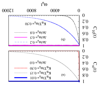
Figure 1: Exponential decay of coherence as a function of dimensionless time $\omega_{u}t$ plotted for (a) detuning energy $\Delta\varepsilon=0.0$ (where largest decoherence is expected) and at values of dimensionless thermal energy ${\rm K_{B}T}/{\omega_{u}}=0.01$ (near boiling point of liquid helium), $=0.15$ (near boiling point of liquid nitrogen), and $=0.5$ (near room temperature); for (b) dimensionless thermal energy ${\rm K_{B}T}/{\omega_{u}}=0.5$ at various detuning energies $\Delta\varepsilon/\omega_{u}$ reflecting different probabilities for resonance. All the plots are at values of adiabaticity $J_{\perp}/{\omega_{u}}=0.5$ and electron-phonon coupling $g=2$ that are realizable in oxide DQDs.

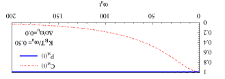
Figure 2: Time dependence, of coherence and population difference, depicting exponential decay of coherence while population remains unchanged for the case of maximum decoherence (i.e., detuning $\Delta\varepsilon=0$) at around room temperature (i.e., ${\rm K_{B}T}/\omega_{u}=0.5$). Adiabaticity $J_{\perp}/{\omega_{u}}=0.5$ and electron-phonon coupling $g=2$ in the plot.

In Fig. 1 (a) we investigate nature of decoherence for zero detuning and various temperatures. At a very low temperature ${\rm K_{B}T}=0.01\omega_{u}$ (i.e., around boiling point of liquid helium), we see that coherence does not decay; whereas, with increasing temperature it decays more rapidly. We compared numerical values of coherence for temperatures $0.01\omega_{u}$, with those at much lower temperatures including $0$ K. Over the entire time range in Fig. 1, with respect to the zero temperature case, we find that the coherence values for ${\rm K_{B}T}=0.01\omega_{u}$ do not change at least up to the twelfth decimal place. This leads us to infer that $\tau>100$ s at these low temperatures (see Table. 1). Similarly, at finite detuning values as well, by contrasting coherence at temperature $0.01\omega_{u}$ with those at much lower temperatures, we report large coherence time $\tau>100$ s in Table. 1. With increasing temperatures, not only do excited phonon states appear with enhanced thermal probability but also the number of degenerate phonon eigenstates increases. Even if the total phonon bath does not exchange excitation with the system (since $\delta\epsilon<<\omega_{u}$), this leads to a fluctuation in local phonon excitations causing destruction of coherence; consequently, there is a decay in coherence while the population difference remains unchanged as shown in Fig. 2. Since there is no exchange of energy between the bath and the polaron, other unoccupied single particle states will not be relevant in producing decoherence. The term $f_{nm}(t)$ in Eq. (6) represents the contributions from degenerate excited phonon eigenstates. At temperatures ${\rm K_{B}T}\ll\omega_{u}$, the phonon ground state (although being probabilistically dominant) produces no decoherence as the strength of decoherence $\mathcal{J}_{00}=0$; furthermore, the next dominant term is proportional to $\sim\exp(-\beta\omega_{u})$ becomes non-negligible only at much higher temperatures (i.e., ${\rm K_{B}T}/\omega_{u}=0.15~{}\&~{}0.5$).

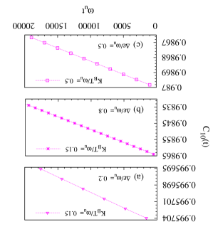
Figure 3: Depiction that exponential decay of coherence is linear at small times. The coherence time is inversely proportional to the slope. The coherence values are averaged over intervals of width between successive points. At a fixed temperature, among the detunings considered, the least decoherence occurs when detuning $\Delta\varepsilon/\omega_{u}=0.5$ since it has the lowest chance for resonance. Figures were drawn at adiabaticity $J_{\perp}/{\omega_{u}}=0.5$ and electron-phonon coupling $g=2$.

To obtain long coherence times even at elevated temperatures, we introduce detuning in the DQD and plot the coherence factor in Fig. 1 (b) at around the room temperature (i.e., ${\rm K_{B}T}=0.5\omega_{u}$). Here, we see that the decoherence time is much longer for $\Delta\varepsilon/\omega_{u}=0.5$ compared to the other two cases $\Delta\varepsilon/\omega_{u}=0.2~{}\&~{}0.8$. The phonon excitation $\bar{\omega}_{n}-\bar{\omega}_{m}=0.2\omega_{u}$ ($\bar{\omega}_{n}-\bar{\omega}_{m}=0.8\omega_{u}$) produces decoherence for $\Delta\varepsilon/\omega_{u}=0.2$ ($\Delta\varepsilon/\omega_{u}=0.8$) case. Given the small phonon frequency window $\omega_{u}-\omega_{l}=0.1\omega_{u}$, as can be seen from Eq. (8), the thermal probability for the phonon excitation $0.8\omega_{u}$ is higher [i.e., $\sim\exp(-\beta\omega_{u})$] compared to that for $0.2\omega_{u}$ [i.e., $\sim\exp(-2\beta\omega_{u})]$. On the other hand, decoherence time for $\Delta\varepsilon/\omega_{u}=0.5$ in Fig. 1 (b) is the longest among all three because the relevant thermal probability $\sim\exp(-4\beta\omega_{u})$ is comparatively smaller.

Next, we plot Fig. 3, by exploiting the linearity of the exponential decay at times much smaller than the large decoherence times realized near boiling point of liquid nitrogen (i.e., ${\rm K_{B}T}=0.15\omega_{u}$) at detuning $\Delta\varepsilon/\omega_{u}=0.2~{}\&~{}0.8$ and for ${\rm K_{B}T}=0.5\omega_{u}$ at $\Delta\varepsilon/\omega_{u}=0.5$. Fig. 3 is in agreement with Fig. 1. The numerical values of coherence times for the cases in Figs. 1 and 3 are reported in Table. 1; at temperatures much above boiling point of liquid helium, we see that with a properly chosen detuning one can get a decoherence time many orders of magnitude larger than the zero-detuning case.

Figure 4: Plot showing coherence decays faster (slower) with increasing adiabaticity $J_{\perp}/{\omega_{u}}$ (electron-phonon coupling $g$) at two representative values of detuning, i.e., $\Delta\varepsilon/\omega_{u}=0.0~{}\&~{}0.2$, and near room temperature.

	${0.0}$	${0.2}$	${0.5}$	${0.8}$
​​​​​​​​​​​​​​​​​​​​​​​​​​​​$0.01$	$>\!\!100$ s	$>\!\!100$ s	$>\!\!100$ s	$>\!\!100$ s
​​​​​​​​​​​​​​​​​​​​​​​​​​$0.15$	50 ps	24 $\mu$s	$>\!0.1$ s	83 ns
​​​​​​​​​​​​​​​​​​​​​​​​​​​​ $0.50$	1 ps	47 ps	​ 0.75 $\mu$s	10 ps

Table 1: Coherence times at various values of scaled thermal energy ${\rm K_{B}T}/\omega_{u}$ and detuning energy $\Delta\varepsilon/\omega_{u}$ when $\hbar\omega_{u}=0.05$ eV.

Lastly, in Fig. 4, we plot the coherence factor for different values of the coupling $g$ and the tunneling amplitude $J_{\perp}$. For a fixed tunneling, coherence is maintained for a longer time when the electron-phonon coupling is stronger. On the other hand, at a fixed value of the coupling, decoherence is enhanced when tunneling increases. These results are consistent with the fact that decoherence diminishes at lower values of the small parameter $\frac{J_{\perp}}{2\sqrt{2}g\omega}$ poldyn ; hcbsite . Comparing Figs. 4 (a) and (b), we again see that finite-detuning provides longer coherence times.

Conclusion.—Although dynamics of a carrier coupled to optical phonons in a Holstein model has been studied recently at both weak and strong couplings vidmar ; eckstein , nevertheless, it has been done for the initial condition where the particle is uncoupled to the phonons in the laboratory frame; furthermore, similar studies need to be conducted for oxide DQD systems.

Our analysis shows that oxides (such as manganites) provide a useful material platform for realizing charge qubits with long coherence times at elevated temperatures (i.e., higher than boiling point of liquid helium). However, experimental confirmation is needed to clearly establish that our oxide variant of double quantum dot has an applicable combination of maneuverability and coherence time; for universal quantum computation, it needs to be demonstrated that high-fidelity gate operations, including two-qubit gate operations, can be performed.

We thank P. B. Littlewood, R. Ramesh. T. V. Ramakrishnan, A. J. Leggett, A. Bhattacharya, M. Manfra, J. Levy, and J. N. Eckstein for stimulating discussions.

Supplemental Material for

“Temperature dependence of long coherence times of oxide charge qubits”

A. Dey and S. Yarlagadda

I Details of the calculation of matrix elements

Here we show the detailed calculations for the matrix elements obtained from the quantum master equation given by Eq. (5) in the main text. The double commutator in Eq. (5) can be broken into four terms. In the equation for the matrix element $\langle 10|\tilde{\rho}_{s}(t)|01\rangle$, the first term on the right-hand side [based on Eq. (5)] is given by

$$\langle 10|\sum_{n}~{}_{ph}\langle n|\tilde{H}_{I}^{L}(t)\tilde{H}_{I}^{L}(\tau)|n\rangle_{ph}\tilde{\rho}_{s}(t)\frac{e^{-\beta\bar{\omega}_{n}}}{Z}|01\rangle = \Big{[}\xi_{+,+}(\mathcal{T})~{}\langle 10|\tilde{c}^{+}_{1}(t)\tilde{c}^{-}_{2}(t)\tilde{c}^{+}_{1}(\tau)\tilde{c}^{-}_{2}(\tau)\tilde{\rho}_{s}(t)|01\rangle$$

$$~{}~{}~{}+\xi_{+,-}(\mathcal{T})~{}\langle 10|\tilde{c}^{+}_{1}(t)\tilde{c}^{-}_{2}(t)\tilde{c}^{+}_{2}(\tau)\tilde{c}^{-}_{1}(\tau)\tilde{\rho}_{s}(t)|01\rangle$$

$$~{}~{}~{}+\xi_{-,+}(\mathcal{T})~{}\langle 10|\tilde{c}^{+}_{2}(t)\tilde{c}^{-}_{1}(t)\tilde{c}^{+}_{1}(\tau)\tilde{c}^{-}_{2}(\tau)\tilde{\rho}_{s}(t)|01\rangle$$

$$~{}~{}~{}+\xi_{-,-}(\mathcal{T})~{}\langle 10|\tilde{c}^{+}_{2}(t)\tilde{c}^{-}_{1}(t)\tilde{c}^{+}_{2}(\tau)\tilde{c}^{-}_{1}(\tau)\tilde{\rho}_{s}(t)|01\rangle\Big{]}.$$

Here, $\mathcal{T}=t-\tau$, i.e., the difference of times at which the the two-time correlation functions $\xi_{\mu,\nu}(\mathcal{T})$ are calculated. The correlation functions can be written as

$$\xi_{\mu,\nu}(\mathcal{T})$$

$$=\frac{1}{4}\sum_{\{n_{k}\}}~{}_{ph}\langle\{n_{k}\}|\tilde{J}^{\mu}_{\perp}(\mathcal{T})\tilde{J}^{\nu}_{\perp}|\{n_{k}\}\rangle_{ph}\frac{e^{-\beta\bar{\omega}_{n}}}{Z}$$

$$=\frac{1}{4}\sum_{\{n_{k}\},\{m_{k}\}}~{}_{ph}\langle\{n_{k}\}|\tilde{J}^{\mu}_{\perp}(\mathcal{T})|\{m_{k}\}\rangle_{ph}~{}_{ph}\langle\{m_{k}\}|\tilde{J}^{\nu}_{\perp}|\{n_{k}\}\rangle_{ph}\frac{e^{-\beta\bar{\omega}_{n}}}{Z}$$

$$=\frac{1}{4}\sum_{\{n_{k}\},\{m_{k}\}}~{}_{ph}\langle\{n_{k}\}|{J}^{\mu}_{\perp}|\{m_{k}\}\rangle_{ph}~{}_{ph}\langle\{m_{k}\}|{J}^{\nu}_{\perp}|\{n_{k}\}\rangle_{ph}e^{i(\bar{\omega}_{n}-\bar{\omega}_{m})\mathcal{T}}\frac{e^{-\beta\bar{\omega}_{n}}}{Z},$$ (S2)

where we observe that

$${{}_{ph}}\langle m_{k}|J^{-}_{\perp}|n_{k}\rangle_{ph}={{}_{ph}}\langle n_{k}|J^{+}_{\perp}|m_{k}\rangle_{ph},$$

$${\rm and}$$

$${{}_{ph}}\langle m_{k}|J^{+}_{\perp}|n_{k}\rangle_{ph}=(-1)^{(n^{k}_{1}+n^{k}_{2}-m^{k}_{1}-m^{k}_{2})}{{}_{ph}}\langle n_{k}|J^{+}_{\perp}|m_{k}\rangle_{ph}.$$

(S3)

Now, we calculate the phonon correlation function $\xi_{+,+}(\mathcal{T})$ below:

$$\!\!\!\!\!\!\!\!\xi_{+,+}(\mathcal{T})$$

$$\!\!\!\!\!\!\!\!=\frac{J^{2}_{\perp}}{4}\Bigg{[}\sum_{\{n_{k}\}}~{}_{ph}\langle\{n_{k}\}|e^{-\frac{1}{\sqrt{N}}\sum_{k}g_{k}[\{a_{1,k}(\mathcal{T})-a^{\dagger}_{1,k}(\mathcal{T})\}-\{a_{2,k}(\mathcal{T})-a^{\dagger}_{2,k}(\mathcal{T})\}]}\times e^{-\frac{1}{\sqrt{N}}\sum_{k}g_{k}[\{a_{1,k}-a^{\dagger}_{1,k}\}-\{a_{2,k}-a^{\dagger}_{2,k}\}]}|\{n_{k}\}\rangle_{ph}\frac{e^{-\beta\bar{\omega}_{n}}}{Z}$$

$$~{}~{}~{}~{}~{}~{}~{}~{}~{}-e^{-\frac{1}{{N}}\sum_{k}g_{k}^{2}{\rm coth}(\frac{\beta\omega_{k}}{2})}\sum_{\{n_{k}\}}~{}_{ph}\langle\{n_{k}\}|e^{-\frac{1}{\sqrt{N}}\sum_{k}g_{k}[\{a_{1,k}-a^{\dagger}_{1,k}\}-\{a_{2,k}-a^{\dagger}_{2,k}\}]}|\{n_{k}\}\rangle_{ph}\frac{e^{-\beta\bar{\omega}_{n}}}{Z}$$

$$~{}~{}~{}~{}~{}~{}~{}~{}~{}-e^{-\frac{1}{{N}}\sum_{k}g_{k}^{2}{\rm coth}(\frac{\beta\omega_{k}}{2})}\sum_{\{n_{k}\}}~{}_{ph}\langle\{n_{k}\}|e^{-\frac{1}{\sqrt{N}}\sum_{k}g_{k}[\{a_{1,k}(\mathcal{T})-a^{\dagger}_{1,k}(\mathcal{T})\}-\{a_{2,k}(\mathcal{T})-a^{\dagger}_{2,k}(\mathcal{T})\}]}|\{n_{k}\}\rangle_{ph}\frac{e^{-\beta\bar{\omega}_{n}}}{Z}$$

$$~{}~{}~{}~{}~{}~{}~{}~{}~{}+e^{-\frac{2}{{N}}\sum_{k}g_{k}^{2}{\rm coth}(\frac{\beta\omega_{k}}{2})}\sum_{\{n_{k}\}}\frac{e^{-\beta\bar{\omega}_{n}}}{Z}\Bigg{]}$$ (S4)

The first term in Eq. (S4) is written as

$$\frac{J^{2}_{\perp}}{4}\sum_{\{n_{k}\}}~{}_{ph}\langle\{n_{k}\}|e^{-\frac{1}{\sqrt{N}}\sum_{k}g_{k}[\{a_{1,k}(\mathcal{T})-a^{\dagger}_{1,k}(\mathcal{T})\}-\{a_{2,k}(\mathcal{T})-a^{\dagger}_{2,k}(\mathcal{T})\}]}\times e^{-\frac{1}{\sqrt{N}}\sum_{k}g_{k}[\{a_{1,k}-a^{\dagger}_{1,k}\}-\{a_{2,k}-a^{\dagger}_{2,k}\}]}|\{n_{k}\}\rangle_{ph}\frac{e^{-\beta\bar{\omega}_{n}}}{Z}$$

$$=\frac{J^{2}_{\perp}}{4}\sum_{\{n^{k}_{1}\}}~{}_{ph}\langle\{n^{k}_{1}\}|e^{-\frac{1}{\sqrt{N}}\sum_{k}g_{k}\{a_{1,k}(\mathcal{T})-a^{\dagger}_{1,k}(\mathcal{T})\}}e^{-\frac{1}{\sqrt{N}}\sum_{k}g_{k}\{a_{1,k}-a^{\dagger}_{1,k}\}}|\{n^{k}_{1}\}\rangle_{ph}\frac{e^{-\beta\bar{\omega}_{n_{1}}}}{Z_{1}}$$

$$~{}~{}~{}~{}~{}~{}~{}\times\sum_{\{n^{k}_{2}\}}~{}_{ph}\langle\{n^{k}_{2}\}|e^{-\frac{1}{\sqrt{N}}\sum_{k}g_{k}\{a_{2,k}(\mathcal{T})-a^{\dagger}_{2,k}(\mathcal{T})\}}e^{-\frac{1}{\sqrt{N}}\sum_{k}g_{k}\{a_{2,k}-a^{\dagger}_{2,k}\}}|\{n^{k}_{2}\}\rangle_{ph}\frac{e^{-\beta\bar{\omega}_{n_{2}}}}{Z_{2}}$$

$$=\frac{J^{2}_{\perp}}{4}e^{-\frac{2}{{N}}\sum_{k}g_{k}^{2}{\rm coth}(\frac{\beta\omega_{k}}{2})[1+{\rm cos}(\omega_{k}\mathcal{T})]}e^{\frac{2}{{N}}i\sum_{k}g_{k}^{2}{\rm sin}(\omega_{k}\mathcal{T})},$$ (S5)

where $Z_{j}=\sum_{\{n^{k}_{j}\}}e^{-\beta\bar{\omega}_{n_{j}}}$ and

$$\sum_{\{n^{k}_{1}\}}~{}_{ph}\langle\{n^{k}_{1}\}|e^{-\frac{1}{\sqrt{N}}\sum_{k}g_{k}\{a_{1,k}(\mathcal{T})-a^{\dagger}_{1,k}(\mathcal{T})\}}e^{-\frac{1}{\sqrt{N}}\sum_{k}g_{k}\{a_{1,k}-a^{\dagger}_{1,k}\}}|\{n^{k}_{1}\}\rangle_{ph}\frac{e^{-\beta\bar{\omega}_{n_{1}}}}{Z_{1}}$$

$$=e^{-\frac{1}{{N}}\sum_{k}g_{k}^{2}}\sum_{\{n^{k}_{1}\}}~{}_{ph}\langle\{n^{k}_{1}\}|e^{\frac{1}{\sqrt{N}}\sum_{k}g_{k}a^{\dagger}_{1,k}e^{i\omega_{k}\mathcal{T}}}e^{-\frac{1}{\sqrt{N}}\sum_{k}g_{k}a_{1,k}e^{-i\omega_{k}\mathcal{T}}}e^{\frac{1}{\sqrt{N}}\sum_{k}g_{k}a^{\dagger}_{1,k}}e^{-\frac{1}{\sqrt{N}}\sum_{k}g_{k}a_{1,k}}|\{n^{k}_{1}\}\rangle_{ph}\frac{e^{-\beta\bar{\omega}_{n_{1}}}}{Z_{1}}$$

$$=e^{-\frac{1}{{N}}\sum_{k}g_{k}^{2}(1+e^{i\omega_{k}\mathcal{T}})}\sum_{\{n^{k}_{1}\}}~{}_{ph}\langle\{n^{k}_{1}\}|e^{\frac{1}{\sqrt{N}}\sum_{k}g_{k}a^{\dagger}_{1,k}(1+e^{i\omega_{k}\mathcal{T}})}e^{-\frac{1}{\sqrt{N}}\sum_{k}g_{k}a_{1,k}(1+e^{i\omega_{k}\mathcal{T}})}|\{n^{k}_{1}\}\rangle_{ph}\frac{e^{-\beta\bar{\omega}_{n_{1}}}}{Z_{1}}$$

$$=e^{-\frac{1}{{N}}\sum_{k}g_{k}^{2}{\rm coth}(\frac{\beta\omega_{k}}{2})(1+{\rm cos}\omega_{k}\mathcal{T})}e^{i\frac{1}{{N}}\sum_{k}g_{k}^{2}{\rm sin}\omega_{k}\mathcal{T}}.$$ (S6)

The second and third terms in Eq. (S4) are written as

$$e^{-\frac{1}{{N}}\sum_{k}g_{k}^{2}{\rm coth}(\frac{\beta\omega_{k}}{2})}\sum_{\{n_{k}\}}~{}_{ph}\langle\{n_{k}\}|e^{-\frac{1}{\sqrt{N}}\sum_{k}g_{k}[\{a_{1,k}-a^{\dagger}_{1,k}\}-\{a_{2,k}-a^{\dagger}_{2,k}\}]}|\{n_{k}\}\rangle_{ph}\frac{e^{-\beta\bar{\omega}_{n}}}{Z}$$

$$=e^{-\frac{1}{{N}}\sum_{k}g_{k}^{2}{\rm coth}(\frac{\beta\omega_{k}}{2})}\sum_{\{n_{k}\}}~{}_{ph}\langle\{n\}|e^{-\frac{1}{\sqrt{N}}\sum_{k}g_{k}[\{a_{1,k}(\mathcal{T})-a^{\dagger}_{1,k}(\mathcal{T})\}-\{a_{2,k}(\mathcal{T})-a^{\dagger}_{2,k}(\mathcal{T})\}]}|\{n_{k}\}\rangle_{ph}\frac{e^{-\beta\bar{\omega}_{n}}}{Z}$$

$$=\frac{J^{2}_{\perp}}{4}e^{-\frac{2}{{N}}\sum_{k}g_{k}^{2}{\rm coth}(\frac{\beta\omega_{k}}{2})}.$$ (S7)

The fourth term in Eq. (S4) is

$$\frac{J^{2}_{\perp}}{4}e^{-\frac{2}{{N}}\sum_{k}g_{k}^{2}{\rm coth}(\frac{\beta\omega_{k}}{2})}\sum_{\{n_{k}\}}\frac{e^{-\beta\bar{\omega}_{n}}}{Z}=\frac{J^{2}_{\perp}}{4}e^{-\frac{2}{{N}}\sum_{k}g_{k}^{2}{\rm coth}(\frac{\beta\omega_{k}}{2})}.$$ (S8)

Finally we get the simplified expression for $\xi_{+,+}(\mathcal{T})$

$$\xi_{+,+}(\mathcal{T})={\kappa}^{2}\Big{[}e^{-\frac{2}{{N}}\sum_{k}g_{k}^{2}{\rm coth}(\frac{\beta\omega_{k}}{2}){\rm cos}(\omega_{k}\mathcal{T})}e^{\frac{2}{{N}}i\sum_{k}g_{k}^{2}{\rm sin}(\omega_{k}\mathcal{T})}-1\Big{]},$$ (S9)

where $\kappa=\frac{J^{\rm mf}_{\perp}}{2}$. In a similar fashion, the other correlation function can be written as

$$\xi_{+,-}(\mathcal{T})={\kappa}^{2}\Big{[}e^{\frac{2}{{N}}\sum_{k}g_{k}^{2}{\rm coth}(\frac{\beta\omega_{k}}{2}){\rm cos}(\omega_{k}\mathcal{T})}e^{-\frac{2}{{N}}i\sum_{k}g_{k}^{2}{\rm sin}(\omega_{k}\mathcal{T})}-1\Big{]}.$$ (S10)

Using Eqs. (S9) and (S10) we write Eq. (LABEL:1st_mntxt_s) as

$$\langle 10|\sum_{n}~{}_{ph}\langle n|\tilde{H}_{I}^{L}(t)\tilde{H}_{I}^{L}(\tau)|n\rangle_{ph}\tilde{\rho}_{s}(t)\frac{e^{-\beta\bar{\omega}_{n}}}{Z}|01\rangle$$

$$=\xi_{+,+}(\mathcal{T})\Big{[}-i\kappa Q(\mathcal{T})\big{(}P(t)P(\tau)+\kappa^{2}Q(\tau)Q(t)\big{)}\langle 01|\tilde{\rho}_{s}(t)|01\rangle+\kappa^{2}Q(\mathcal{T})\big{(}Q(t)P^{*}(\tau)-P(t)Q(\tau)\big{)}\langle 10|\tilde{\rho}_{s}(t)|01\rangle\Big{]}$$

$$~{}+\xi_{+,-}(\mathcal{T})\Big{[}i\kappa(Q(t)P^{*}(\mathcal{T})P(\tau)-Q(\tau)P(t)P(\mathcal{T}))\langle 01|\tilde{\rho}_{s}(t)|01\rangle+\big{(}\kappa^{2}Q(t)Q(\tau)P^{*}(\mathcal{T})+P(t)P(\mathcal{T})P^{*}(\tau)\big{)}\langle 10|\tilde{\rho}_{s}(t)|01\rangle\Big{]}.$$

(S11)

The evolution of the system parts of the right-hand side of Eq. (LABEL:1st_mntxt_s) can be calculated using the following relations:

$$e^{-iH_{s}^{L}t}|10\rangle = [P(t)^{*}|10\rangle-i\kappa Q(t)|01\rangle]e^{i\frac{J_{\parallel}}{4}t},$$ (S12)

and

$$e^{-iH_{s}^{L}t}|01\rangle = [P(t)|01\rangle-i\kappa Q(t)|10\rangle]e^{i\frac{J_{\parallel}}{4}t},$$ (S13)

with $P(t)=\rm{cos}\Big{(}t\sqrt{\frac{\Delta\varepsilon^{2}}{4}+\kappa^{2}}\Big{)}+i\frac{\Delta\varepsilon}{2}\frac{\rm{sin}\Big{(}t\sqrt{\frac{\Delta\varepsilon^{2}}{4}+\kappa^{2}}\Big{)}}{\sqrt{\frac{\Delta\varepsilon^{2}}{4}+\kappa^{2}}}$ and $Q(t)=\frac{\rm{sin}\Big{(}t\sqrt{\frac{\Delta\varepsilon^{2}}{4}+\kappa^{2}}\Big{)}}{\sqrt{\frac{\Delta\varepsilon^{2}}{4}+\kappa^{2}}}$. For $\kappa\ll\Delta\varepsilon$, we can approximate Eq. (S11) as

$$\langle 10|\sum_{n}~{}_{ph}\langle n|\tilde{H}_{I}^{L}(t)\tilde{H}_{I}^{L}(\tau)|n\rangle_{ph}\tilde{\rho}_{s}(t)\frac{e^{-\beta\bar{\omega}_{n}}}{Z}|01\rangle = \xi_{+,-}(\mathcal{T})P(t)P(\mathcal{T})P^{*}(\tau)\langle 10|\tilde{\rho}_{s}(t)|01\rangle$$ (S14)

$$= \xi_{+,-}(\mathcal{T})e^{i\Delta\varepsilon\mathcal{T}}\langle 10|\tilde{\rho}_{s}(t)|01\rangle.$$

The second term is given by

$$\langle 10|\sum_{n}~{}_{ph}\langle n|\tilde{H}_{I}^{L}(t)\tilde{\rho}_{s}(t)\otimes R_{0}\tilde{H}_{I}^{L}(\tau)|n\rangle_{ph}|01\rangle$$

$$=\xi_{+,+}(-\mathcal{T})\Big{[}\langle 10|\tilde{\rho}_{s}(t)|10\rangle\big{(}-i\kappa P(t)P^{2}(\tau)Q(t)+i\kappa^{3}Q(t)Q^{2}(\tau)P^{*}(t)\big{)}$$

$$~{}~{}~{}~{}~{}~{}~{}+\langle 10|\tilde{\rho}_{s}(t)|01\rangle\big{(}\kappa^{2}P(t)P(\tau)Q(t)Q(\tau)+\kappa^{2}Q(t)Q(\tau)P^{*}(t)P^{*}(\tau)\big{)}$$

$$~{}~{}~{}~{}~{}~{}~{}+\langle 01|\tilde{\rho}_{s}(t)|10\rangle\big{(}P^{2}(t)P^{2}(\tau)+\kappa^{4}Q^{2}(t)Q^{2}(\tau)\big{)}$$

$$~{}~{}~{}~{}~{}~{}~{}+\langle 01|\tilde{\rho}_{s}(t)|01\rangle\big{(}i\kappa P^{2}(t)P(\tau)Q(\tau)-i\kappa^{3}Q^{2}(t)Q(\tau)P^{*}(\tau)\big{)}\Big{]}$$

$$~{}~{}~{}+\xi_{+,-}(-\mathcal{T})\Big{[}\langle 10|\tilde{\rho}_{s}(t)|10\rangle\big{(}-i\kappa^{3}P(t)Q(t)Q^{2}(\tau)+i\kappa Q(t)P^{*}(t)P^{2}(\tau)\big{)}$$

$$~{}~{}~{}~{}~{}~{}~{}+\langle 10|\tilde{\rho}_{s}(t)|01\rangle\big{(}-\kappa^{2}P(t)P^{*}(\tau)Q(t)Q(\tau)-\kappa^{2}Q(t)P^{*}(t)Q(\tau)P(\tau)\big{)}$$

$$~{}~{}~{}~{}~{}~{}~{}+\langle 01|\tilde{\rho}_{s}(t)|10\rangle\big{(}\kappa^{2}P^{2}(t)Q^{2}(\tau)+\kappa^{2}Q^{2}(t)P^{2}(\tau)\big{)}$$

$$~{}~{}~{}~{}~{}~{}~{}+\langle 01|\tilde{\rho}_{s}(t)|01\rangle\big{(}i\kappa^{3}Q^{2}(t)Q(\tau)P(\tau)-i\kappa P^{2}(t)P^{*}(\tau)Q(\tau)\big{)}\Big{]}.$$ (S15)

For $\kappa\ll\Delta\varepsilon$, we get

$$\langle 10|\sum_{n}~{}_{ph}\langle n|\tilde{H}_{I}^{L}(\tau)\tilde{\rho}_{s}(t)\otimes R_{0}\tilde{H}_{I}^{L}(t)|n\rangle_{ph}|01\rangle = \xi_{+,+}(-\mathcal{T})\langle 01|\tilde{\rho}_{s}(t)|10\rangle P^{2}(t)P^{2}(\tau)$$ (S16)

$$= \xi_{+,+}(-\mathcal{T})\langle 01|\tilde{\rho}_{s}(t)|10\rangle e^{i\Delta\varepsilon(t+\tau)}.$$

The third term is expressed as

$$\langle 10|\sum_{n}~{}_{ph}\langle n|\tilde{H}_{I}^{L}(\tau)\tilde{\rho}_{s}(t)\otimes R_{0}\tilde{H}_{I}^{L}(t)|n\rangle_{ph}|01\rangle$$

$$=\xi_{+,+}(\mathcal{T})\Big{[}\langle 10|\tilde{\rho}_{s}(t)|10\rangle\big{(}-i\kappa P(\tau)P^{2}(t)Q(\tau)+i\kappa^{3}Q(\tau)Q^{2}(t)P^{*}(\tau)\big{)}$$

$$~{}~{}~{}~{}~{}~{}~{}+\langle 10|\tilde{\rho}_{s}(t)|01\rangle\big{(}\kappa^{2}P(\tau)P(t)Q(t)Q(\tau)+\kappa^{2}Q(\tau)Q(t)P^{*}(\tau)P^{*}(t)\big{)}$$

$$~{}~{}~{}~{}~{}~{}~{}+\langle 01|\tilde{\rho}_{s}(t)|10\rangle\big{(}P^{2}(\tau)P^{2}(t)+\kappa^{4}Q^{2}(\tau)Q^{2}(t)\big{)}$$

$$~{}~{}~{}~{}~{}~{}~{}+\langle 01|\tilde{\rho}_{s}(t)|01\rangle\big{(}i\kappa P^{2}(\tau)P(t)Q(t)-i\kappa^{3}Q^{2}(\tau)Q(t)P^{*}(t)\big{)}\Big{]}$$

$$~{}~{}~{}+\xi_{+,-}(\mathcal{T})\Big{[}\langle 10|\tilde{\rho}_{s}(t)|10\rangle\big{(}-i\kappa^{3}P(\tau)Q(\tau)Q^{2}(t)+i\kappa Q(\tau)P^{*}(\tau)P^{2}(t)\big{)}$$

$$~{}~{}~{}~{}~{}~{}~{}+\langle 10|\tilde{\rho}_{s}(t)|01\rangle\big{(}-\kappa^{2}P(\tau)P^{*}(t)Q(\tau)Q(t)-\kappa^{2}Q(\tau)P^{*}(\tau)Q(t)P(t)\big{)}$$

$$~{}~{}~{}~{}~{}~{}~{}+\langle 01|\tilde{\rho}_{s}(t)|10\rangle\big{(}\kappa^{2}P^{2}(\tau)Q^{2}(t)+\kappa^{2}Q^{2}(\tau)P^{2}(t)\big{)}$$

$$~{}~{}~{}~{}~{}~{}~{}+\langle 01|\tilde{\rho}_{s}(t)|01\rangle\big{(}i\kappa^{3}Q^{2}(\tau)Q(t)P(t)-i\kappa P^{2}(\tau)P^{*}(t)Q(t)\big{)}\Big{]}.$$ (S17)

For $\kappa\ll\Delta\varepsilon$, we obtain

$$\langle 10|\sum_{n}~{}_{ph}\langle n|\tilde{H}_{I}^{L}(\tau)\tilde{\rho}_{s}(t)\otimes R_{0}\tilde{H}_{I}^{L}(t)|n\rangle_{ph}|01\rangle = \xi_{+,+}(\mathcal{T})\langle 01|\tilde{\rho}_{s}(t)|10\rangle P^{2}(\tau)P^{2}(t)$$ (S18)

$$= \xi_{+,+}(\mathcal{T})\langle 01|\tilde{\rho}_{s}(t)|10\rangle e^{i\Delta\varepsilon(t+\tau)}.$$

Lastly, the fourth term reads

$$\langle 10|\sum_{n}~{}\tilde{\rho}_{s}(t)\frac{e^{-\beta\bar{\omega}_{n}}}{Z}_{ph}\langle n|\tilde{H}_{I}^{L}(\tau)\tilde{H}_{I}^{L}(t)|n\rangle_{ph}|01\rangle$$

$$=\xi_{+,+}(-\mathcal{T})\Big{[}i\kappa Q(\mathcal{T})\big{(}P(t)P(\tau)+\kappa^{2}Q(\tau)Q(t)\big{)}\langle 10|\tilde{\rho}_{s}(t)|10\rangle+\kappa^{2}Q(\mathcal{T})\big{(}Q(t)P^{*}(\tau)-P(t)Q(\tau)\big{)}\langle 10|\tilde{\rho}_{s}(t)|01\rangle\Big{]}$$

$$~{}+\xi_{+,-}(-\mathcal{T})\Big{[}i\kappa(-Q(t)P^{*}(\mathcal{T})P(\tau)+Q(\tau)P(t)P(\mathcal{T}))\langle 10|\tilde{\rho}_{s}(t)|10\rangle+\big{(}\kappa^{2}Q(t)Q(\tau)P^{*}(\mathcal{T})+P(t)P(\mathcal{T})P^{*}(\tau)\big{)}\langle 10|\tilde{\rho}_{s}(t)|01\rangle\Big{]}.$$

(S19)

For $\kappa\ll\Delta\varepsilon$, we can approximate the above expression as

$$\langle 10|\sum_{n}~{}\tilde{\rho}_{s}(t)\frac{e^{-\beta\bar{\omega}_{n}}}{Z}_{ph}\langle n|\tilde{H}_{I}^{L}(\tau)\tilde{H}_{I}^{L}(t)|n\rangle_{ph}|01\rangle = \xi_{+,-}(-\mathcal{T})P(t)P(\mathcal{T})P^{*}(\tau)\langle 10|\tilde{\rho}_{s}(t)|01\rangle$$ (S20)

$$= \xi_{+,-}(-\mathcal{T})e^{i\Delta\varepsilon\mathcal{T}}\langle 10|\tilde{\rho}_{s}(t)|01\rangle.$$

Putting Eqs. (S14), (S16), (S18), and (S20) in Eq. (5) of the main text and using the equalities in Eq. (S3), one obtains Eq. (8) in the main text. In a similar way, one can deduce Eq. (9) for the diagonal element. Eqs. (6) and (7) can be deduced by using Eqs. (S11), (S15), (S17), and (S19) without the approximation $\kappa\ll\Delta\varepsilon$ and re-expressing the terms in {$|\epsilon_{s}\rangle$, $|\epsilon_{t}\rangle$} basis. It should be noted that, at zero detuning, the only system excitation is given by $\delta\epsilon=2\kappa=J^{\rm mf}_{\perp}$.

References

• (1) T. Hayashi, T. Fujisawa, H. D. Cheong, Y. H. Jeong, and Y. Hirayama, Phys. Rev. Lett. 91, 226804 (2003).
• (2) T. Fujisawa, T. Hayashi, and S. Sasaki, Rep. Prog. Phys. 69, 759 (2006).
• (3) J. R. Petta, A. C. Johnson, C. M. Marcus, M. P. Hanson, and A. C. Gossard, Phys. Rev. Lett. 93, 186802 (2004).
• (4) G. Shinkai, T. Hayashi, T. Ota, and T. Fujisawa, Phys. Rev. Lett. 103, 056802 (2009).
• (5) K. D. Petersson, C. G. Smith, D. Anderson, P. Atkinson, G. A. C. Jones, and D. A. Ritchie, Phys. Rev. Lett. 103, 016805 (2009).
• (6) K. D. Petersson, C. G. Smith, D. Anderson, P. Atkinson, G. A. C. Jones, and D. A. Ritchie, Nano Lett. 10, 2789 (2010)
• (7) K. D. Petersson, J. R. Petta, H. Lu, and A. C. Gossard, Phys. Rev. Lett. 105, 246804 (2010).
• (8) G. Cao, H. O. Li, T. Tu, L. Wang, C. Zhou, M. Xiao, G. C. Guo, H. W. Jiang, and G. P. Guo, Nat. Commun. 4, 1401 (2013).
• (9) H. O. Li, G. Cao, G. D. Yu, M. Xiao, G. C. Guo, H. W. Jiang, and G. P. Guo, Nat. Commun. 6, 7681 (2015).
• (10) Z. Shi, C. B. Simmons, D. R. Ward, J. R. Prance, R. T. Mohr, T. S. Koh, J. K. Gamble, X. Wu, D. E. Savage, M. G. Lagally, M. Friesen, S. N. Coppersmith, and M. A. Eriksson, Phys. Rev. B 88, 075416 (2013).
• (11) D. Kim, D. R. Ward, C. B. Simmons, J. K. Gamble, R. Blume-Kohout, E. Nielsen, D. E. Savage, M. G. Lagally, M. Friesen, S. N. Coppersmith, and M. A. Eriksson, Nat. Nanotechnol. 10, 243 (2015).
• (12) E. Dagotto and Y. Tokura “A brief introduction to strongly correlated electronic materials” in Multifunctional Oxide Heterostructures edited by E. Tsymbal, C.B. Eom, R. Ramesh and E. Dagotto (Oxford University Press, 2012).
• (13) Y. Tokura and H. Y. Hwang, Nature Materials 7 694 (2008).
• (14) J. Ngai, F. Walker and C. Ahn, Annual Review of Materials Research, 44, 1 (2014).
• (15) C.H. Ahn, A. Bhattacharya, M. Di Ventra, J.N. Eckstein, C. Daniel Frisbie, M.E. Gershenson, A.M. Goldman, I.H. Inoue, J. Mannhart, Andrew J. Millis, Alberto F. Morpurgo, Douglas Natelson, and Jean-Marc Triscone, Rev. Mod. Phys. 784, 1185 (2006).
• (16) M. Schlosshauer, Rev. Mod. Phys. 76, 1267 (2005).
• (17) W. H. Zurek, Rev. Mod. Phys. 75, 715 (2003).
• (18) T. Holstein, Ann. Phys. (N. Y.), 8, 343 (1959).
• (19) A. S. Alexandrov, Phys. Rev. B 61, 12315 (2000).
• (20) S. Yarlagadda, Phys. Rev. B 62, 14828 (2000).
• (21) W. G. van der Wiel, S. De Franceschi, J. M. Elzerman, T. Fujisawa, S. Tarucha, and L. P. Kouwenhoven, Rev. Mod. Phys. 75, 1 (2002).
• (22) I. G. Lang and Y. A. Firsov, Zh. Eksp. Teor. Fiz. 43, 1843 (1962) [Sov. Phys. JETP 16, $1301$ ($1963$)].
• (23) A. Dey, M. Q. Lone, and S. Yarlagadda, Phys. Rev. B 92, 094302 (2015).
• (24) A. Dey and S. Yarlagadda, Phys. Rev. B 89, 064311 (2014).
• (25) H. P. Beuer and F. Petruccione, The Theory of Open Quantum systems (Oxford University Press, Oxford, 2002).
• (26) See Supplemental material at […] for detailed calculations of the four matrix elements obtained from the quantum-master equation.
• (27) A. Lanzara, N. L. Saini, M. Brunelli, F. Natali, A. Bianconi, P. G. Radaelli, and S.-W. Cheong, Phys. Rev. Lett. 81, 878 (1998).
• (28) A. J. Millis, P. B. Littlewood, and B. I. Shraiman, Phys. Rev. Lett. 74, 5144 (1995).
• (29) T. F. Seman, K. H. Ahn, T. Lookman, A. Saxena, A. R. Bishop, and P. B. Littlewood, Phys. Rev. B 86, 184106 (2012).
• (30) S. R. Wilkinson, C. F. Varucha, M. C. Fischer, K. W. Madison, P. R. Morrow, Q. Niu, B. Sundaram, and M. G. Raizen, Nat. Phys. 387, 575 (1997).
• (31) F. Dorfner, L. Vidmar, C. Brockt, E. Jeckelmann, and F. Heidrich-Meisner, Phys. Rev. B 91, 104302 (2015).
• (32) S. Sayyad and M. Eckstein, Phys. Rev. B 91, 104301 (2015).