Distortion Varieties

Abstract

The distortion varieties of a given projective variety are parametrized by duplicating coordinates and multiplying them with monomials. We study their degrees and defining equations. Exact formulas are obtained for the case of one-parameter distortions. These are based on Chow polytopes and Gröbner bases. Multi-parameter distortions are studied using tropical geometry. The motivation for distortion varieties comes from multi-view geometry in computer vision. Our theory furnishes a new framework for formulating and solving minimal problems for camera models with image distortion.

1 Introduction

This article introduces a construction in algebraic geometry that is motivated by multi-view geometry in computer vision. In that field, one thinks of a camera as a linear projection $\mathbb{P}^{3}\dashrightarrow\mathbb{P}^{2}$, and a model is a projective variety $X\subset\mathbb{P}^{n}$ that represents the relative positions of two or more such cameras. The data are correspondences of image points in $\mathbb{P}^{2}$. These define a linear subspace $L\subset\mathbb{P}^{n}$, and the task is to compute the real points in the intersection $L\cap X$ as fast and accurately as possible. See [20, Chapter 9] for a textbook introduction.

A model for cameras with image distortion allows for an additional unknown parameter $\lambda$. Each coordinate of $X$ gets multiplied by a polynomial in $\lambda$ whose coefficients also depend on the data. We seek to estimate both $\lambda$ and the point in $X$, where the data now specify a subspace $L^{\prime}$ in a larger projective space $\mathbb{P}^{N}$. The distortion variety $X^{\prime}$ lives in that $\mathbb{P}^{N}$, it satisfies ${\rm dim}(X^{\prime})={\rm dim}(X)+1$, and the task is to compute $L^{\prime}\cap X^{\prime}$ in $\mathbb{P}^{N}$ fast and accurately.

We illustrate the idea of distortion varieties for the basic scenario in two-view geometry.

Example 1.1.

The relative position of two uncalibrated cameras is expressed by a $3{\times}3$-matrix $x=(x_{ij})$ of rank $2$, known as the fundamental matrix. Let $n=8$ and write $F$ for the hypersurface in $\mathbb{P}^{8}$ defined by the $3\times 3$-determinant. Seven (generic) image correspondences in two views determine a line $L$ in $\mathbb{P}^{8}$, and one rapidly computes the three points in $L\cap F$.

The $8$-point radial distortion problem [26, Section 7.1.3] is modeled as follows in our setting. We duplicate the coordinates in the last row and last column of $x$, and we set

$$\begin{matrix}\left(x_{11}:x_{12}:x_{13}:y_{13}:x_{21}:x_{22}:x_{23}:y_{23}:x_{31}:y_{31}:x_{32}:y_{32}:x_{33}:y_{33}:z_{33}\right)\,\,\,\,=\qquad\quad\qquad\\ \left(x_{11}:x_{12}:x_{13}:x_{13}\lambda:x_{21}:x_{22}:x_{23}:x_{23}\lambda:x_{31}:x_{31}\lambda:x_{32}:x_{32}\lambda:x_{33}:x_{33}\lambda:x_{33}\lambda^{2}\right).\end{matrix}$$ (1)

Here $N=14$. The distortion variety $F^{\prime}$ is the closure of the set of matrices (1) where $x\in F$ and $\lambda\in\mathbb{C}$. The variety $F^{\prime}$ has dimension $8$ and degree $16$ in $\mathbb{P}^{14}$, whereas $F$ has dimension $7$ and degree $3$ in $\mathbb{P}^{8}$. To estimate both $\lambda$ and the relative camera positions, we now need eight image correspondences. These data specify a linear space $L^{\prime}$ of dimension $6$ in $\mathbb{P}^{14}$. The task in the computer vision application is to rapidly compute the $16$ points in $L^{\prime}\cap F^{\prime}$.

The prime ideal of the distortion variety $F^{\prime}$ is minimally generated by $18$ polynomials in the $15$ variables. First, there are $15$ quadratic binomials, namely the $2\times 2$-minors of matrix

$$\begin{pmatrix}x_{13}&x_{23}&x_{31}&x_{32}&x_{33}&y_{33}\\ y_{13}&y_{23}&y_{31}&y_{32}&y_{33}&z_{33}\end{pmatrix}.$$ (2)

Note that this matrix has rank $1$ under the substitution (1). Second, there are three cubics

$$\begin{matrix}x_{11}x_{22}x_{33}-x_{11}x_{23}x_{32}-x_{12}x_{21}x_{33}+x_{12}x_{23}x_{31}+x_{13}x_{21}x_{32}-x_{13}x_{22}x_{31},\\ x_{13}x_{22}y_{31}-x_{12}x_{23}y_{31}-x_{13}x_{21}y_{32}+x_{11}x_{23}y_{32}+x_{12}x_{21}y_{33}-x_{11}x_{22}y_{33},\\ x_{22}y_{13}y_{31}-x_{12}y_{23}y_{31}-x_{21}y_{13}y_{32}+x_{11}y_{23}y_{32}+x_{12}x_{21}z_{33}-x_{11}x_{22}z_{33}.\end{matrix}$$ (3)

These three $3\times 3$-determinants replicate the equation that defines the original model $F$. $\diamondsuit$

This paper is organized as follows. Section 2 introduces the relevant concepts and definitions from computer vision and algebraic geometry. We present camera models with image distortion, with focus on distortions with respect to a single parameter $\lambda$. The resulting distortion varieties $X_{[u]}$ live in the rational normal scroll $\mathcal{S}_{u}$, where $u=(u_{0},u_{1},\ldots,u_{n})$ is a vector of non-negative integers. This distortion vector indicates that the coordinate $x_{i}$ on $\mathbb{P}^{n}$ is replicated $u_{i}$ times when passing to $\mathbb{P}^{N}$. In Example 1.1 we have $u=(0,0,1,0,0,1,1,1,2)$ and $\mathcal{S}_{u}$ is the $9$-dimensional rational normal scroll defined by the $2\times 2$-minors of (2).

Our results on one-parameter distortions of arbitrary varieties are stated and proved in Section 3. Theorem 3.2 expresses the degree of $X_{[u]}$ in terms of the Chow polytope of $X$. Theorem 3.10 derives ideal generators for $X_{[u]}$ from a Gröbner basis of $X$. These results explain what we observed in Example 1.1, namely the degree $16$ and the equations in (2)-(3).

Section 4 deals with multi-parameter distortions. We first derive various camera models that are useful for applications, and we then present the relevant algebraic geometry.

Section 5 is concerned with a concrete application to solving minimal problems in computer vision. We focus on the distortion variety f+E+$\lambda$ of degree $23$ derived in Section 2.

2 One-Parameter Distortions

This section has three parts. First, we derive the relevant camera models from computer vision. Second, we introduce the distortion varieties $X_{[u]}$ of an arbitrary projective variety $X$. And, third, we study the distortion varieties for the camera models from the first part.

2.1 Multi-view geometry with image distortion

A perspective camera in computer vision [20, pg 158] is a linear projection $\mathbb{P}^{3}\dashrightarrow\mathbb{P}^{2}$. The $3\times 4$-matrix that represents this map is written as $\,K\cdot\left(\!\!\begin{array}[]{c}R\,|\,t\end{array}\!\!\right)$ where $R\in\textup{SO}(3)$, $t\in\mathbb{R}^{3}$, and $K$ is an upper-triangular $3\times 3$ matrix known as the calibration matrix. This transforms a point $X\in\mathbb{P}^{3}$ from the world Cartesian coordinate system to the camera Cartesian coordinate system. Here, we usually normalize homogeneous coordinates on $\mathbb{P}^{3}$ and $\mathbb{P}^{2}$ so that the last coordinate equals $1$. With this, points in $\mathbb{R}^{3}$ map to $\mathbb{R}^{2}$ under the action of the camera.

The following camera model was introduced in [28, Eqn 3] to deal with image distortions:

$$\quad\alpha\,\left(\!\!\begin{array}[]{c}R\,|\,t\end{array}\!\!\right)\,X\,\,=\,\,\left(\!\!\begin{array}[]{l}h(\|A\,U+b\|)\,(A\,U+b)\\ g(\|A\,U+b\|)\end{array}\!\!\right)\qquad\mbox{for some}\,\,\,\alpha\in\mathbb{R}\backslash\{0\}.$$ (4)

The two functions $h\colon\mathbb{R}\to\mathbb{R}$ and $g\colon\mathbb{R}\to\mathbb{R}$ represent the distortion. The invertible matrix $A\in\mathbb{R}^{2\times 2}$ and the vector $b\in\mathbb{R}^{2}$ are used to transform the image point $U\in\mathbb{R}^{2}$ into the image Cartesian coordinate system. The perspective camera in the previous paragraph is obtained by setting $h=g=1$ and taking the calibration matrix $K$ to be the inverse of $\left(\!\!\begin{array}[]{cc}A&b\\ 0\,0&1\end{array}\!\!\right)$.

Micusik and Pajdla [28] studied applications to fish eye lenses as well as catadioptric cameras. In this context they found that it often suffices to fix $h=1$ and to take a quadratic polynomial for $g$. For the following derivation we choose $g(t)=1+\mu t^{2}$, where $\mu$ is an unknown parameter. We also assume that the calibration matrix has the diagonal form $K=\mbox{diag}{\bigl{[}f,f,1\bigr{]}}$. If we set $\,\lambda=\mu/f^{2}\,$ then the model (4) simplifies to

$$\quad\alpha\,\left(\!\!\begin{array}[]{c}R\,|\,t\end{array}\!\!\right)\,X\,\,=\,\,K^{-1}\left(\!\!\begin{array}[]{l}\quad U\\ 1+\lambda\|U\|^{2}\end{array}\!\!\right)\qquad\mbox{for some}\,\,\,\alpha\in\mathbb{R}\backslash\{0\}.$$ (5)

Let us now analyze two-view geometry for the model (5). The quantity $\,\lambda=\mu/f^{2}$ is our distortion parameter. Throughout the discussion in Section 2 there is only one such parameter. Later, in Section 4, there will be two or more different distortion parameters.

Following [20, §9.6] we represent two camera matrices $\left(\!\!\begin{array}[]{c}R_{1}\,|\,t_{1}\end{array}\!\!\right)$ and $\left(\!\!\begin{array}[]{c}R_{2}\,|\,t_{2}\end{array}\!\!\right)$ by their essential matrix $\,E$. This $3\times 3$-matrix has rank $2$ and satisfies the Demazure equations. The equations were first derived in [10]; they take the matrix form $2\,E\,E^{\top}E-\mbox{trace}{(E\,E^{\top})}E=0$. For a pair $(U_{1},U_{2})$ of corresponding points in two images, the epipolar constraint now reads

$$0\,=\,\left(\!\!\begin{array}[]{c}AU_{2}\\ 1+\mu\|AU_{2}\|^{2}\end{array}\!\!\right)^{\!\!\top}\!\!E\,\left(\!\!\begin{array}[]{c}AU_{1}\\ \!1+\mu\|AU_{1}\|^{2}\end{array}\!\!\right)\,=\,\left(\!\!\begin{array}[]{c}U_{2}\\ \!1+\lambda\|U_{2}\|^{2}\!\end{array}\!\!\right)^{\!\!\top}\!\!K^{-\top}E\,K^{-1}\left(\!\!\begin{array}[]{c}U_{1}\\ 1+\lambda\|U_{1}\|^{2}\!\end{array}\!\!\right).$$ (14)

In this way, the essential matrix $E$ expresses a necessary condition for two points $U_{1}$ and $U_{2}$ in the image planes to be pictures of the same world point. The fundamental matrix is obtained from the essential matrix and the calibration matrix:

$$F\,=\,\left(\!\!\begin{array}[]{ccc}f_{11}&f_{12}&f_{13}\\ f_{21}&f_{22}&f_{23}\\ f_{31}&f_{32}&f_{33}\end{array}\!\!\right)\,\,\,=\,\,\,K^{-\top}E\,K^{-1}.$$ (15)

Using the coordinates of $U_{1}=[u_{1},v_{1}]^{\top}$ and $U_{2}=[u_{2},v_{2}]^{\top}$, the epipolar constraint (14) is

$$0\! \!=\! u_{2}u_{1}f_{11}+u_{2}v_{1}f_{12}+u_{2}f_{13}+u_{2}\|U_{1}\|^{2}\lambda f_{13}+v_{2}u_{1}f_{21}+v_{2}v_{1}f_{22}+v_{2}f_{23}+v_{2}\|U_{1}\|^{2}\lambda f_{23}+$$

$$u_{1}f_{31}+u_{1}\|U_{2}\|^{2}\lambda f_{31}+v_{1}f_{32}+v_{1}\|U_{2}\|^{2}\lambda f_{32}+f_{33}+(\|U_{1}\|^{2}{+}\|U_{2}\|^{2})\lambda f_{33}+\|U_{1}\|^{2}\|U_{2}\|^{2}\lambda^{2}f_{33}.$$

This is a sum of $15$ terms. The corresponding monomials in the unknowns form the vector

$$m^{\top}=\left[f_{11},f_{12},f_{13},f_{13}\lambda,f_{21},f_{22},f_{23},f_{23}\lambda,f_{31},f_{31}\lambda,f_{32},f_{32}\lambda,f_{33},f_{33}\lambda,f_{33}\lambda^{2}\right].$$ (16)

The $15$ coefficients are real numbers given by the data. The coefficient vector $c$ is equal to

$$\left[u_{2}u_{1},u_{2}v_{1},u_{2},u_{2}\|U_{1}\|^{2}\!\!,v_{2}u_{1},v_{2}v_{1},v_{2},v_{2}\|U_{1}\|^{2}\!\!,u_{1},u_{1}\|U_{2}\|^{2}\!\!,v_{1},v_{1}\|U_{2}\|^{2}\!\!,1,\|U_{1}\|^{2}{+}\|U_{2}\|^{2}\!\!,\|U_{1}\|^{2}\|U_{2}\|^{2}\right]^{\!\top}_{.}$$

With this notation, the epipolar constraint given by one point correspondence is simply

$$c^{\top}m\,\,=\,\,0.$$ (17)

At this stage we have derived the distortion variety in Example 1.1. Identifying $f_{ij}$ with the variables $x_{ij}$, the vector (16) is precisely the same as that in (1). This is the parametrization of the rational normal scroll $\mathcal{S}_{u}$ in $\mathbb{P}^{14}$ where $u=(0,0,1,0,0,1,1,1,2)$. The set of fundamental matrices is dense in the hypersurface $X=\{{\rm det}(F)=0\}$ in $\mathbb{P}^{8}$. Its distortion variety $X_{[u]}$ has dimension $8$ and degree $16$ in $\mathbb{P}^{14}$. Each point correspondence $(U_{1},U_{2})$ determines a vector $c$ and hence a hyperplane in $\mathbb{P}^{14}$. The constraint (17) means intersecting $X_{[u]}$ with that hyperplane. Eight point correspondences determine a $6$-dimensional linear space in $\mathbb{P}^{14}$. Intersecting $X_{[u]}$ with that linear subspace is the same as solving the $8$-point radial distortion problem in [26, Section 7.1.3]. The expected number of complex solutions is $16$.

2.2 Scrolls and Distortions

This subsection introduces the algebro-geometric objects studied in this paper. We fix a non-zero vector $u=(u_{0},u_{1},\ldots,u_{n})\in\mathbb{N}^{n+1}$ of non-negative integers, we abbreviate $|u|=u_{0}+u_{1}+\cdots+u_{n}$, and we set $N=|u|+n$. The rational normal scroll $\,\mathcal{S}_{u}$ is a smooth projective variety of dimension $n+1$ and degree $|u|$ in $\mathbb{P}^{N}$. It has the parametric representation

$$\!\!\bigl{(}x_{0}:x_{0}\lambda:x_{0}\lambda^{2}:\cdots:x_{0}\lambda^{u_{0}}:x_{1}:x_{1}\lambda:x_{1}\lambda^{2}:\cdots:x_{1}\lambda^{u_{1}}:\,\cdots:x_{n}:x_{n}\lambda:\cdots:x_{n}\lambda^{u_{n}}\bigr{)}.$$ (18)

The coordinates are monomials, so the scroll $\mathcal{S}_{u}$ is also a toric variety [8]. Since ${\rm degree}(\mathcal{S}_{u})=|u|$ equals ${\rm codim}(\mathcal{S}_{u})+1=N-n+1$, it is a variety of minimal degree [19, Example 1.14].

Restriction to the coordinates $(x_{0}:x_{1}:\cdots:x_{n})$ defines a rational map $\mathcal{S}_{u}\dashrightarrow\mathbb{P}^{n}$. This is a toric fibration [11]. Its fibers are curves parametrized by $\lambda$. The base locus is a coordinate subspace $\mathbb{P}^{n}\subset\mathbb{P}^{N}$. Its points have support on the last coordinate in each of the $n+1$ groups. For instance, in Example 2.1 the base locus is the $\mathbb{P}^{2}$ defined by $\langle a_{0},b_{0},b_{1},c_{0},c_{1},c_{2}\rangle$ in $\mathbb{P}^{8}$.

The prime ideal of the scroll $\mathcal{S}_{u}$ is generated by the $2\times 2$-minors of a $2\times|u|$-matrix of unknowns that is obtained by concatenating Hankel matrices on the blocks of unknowns; see [12, Lemma 2.1], [31], and Example 2.1 below. For a textbook reference see [19, Theorem 19.9].

We now consider an arbitrary projective variety $X$ of dimension $d$ in $\mathbb{P}^{n}$. This is the underlying model in some application, such as computer vision. We define the distortion variety of level $u$, denoted $X_{[u]}$, to be the closure of the preimage of $X$ under the map $\mathcal{S}_{u}\dashrightarrow\mathbb{P}^{n}$. The fibers of this map are curves. The distortion variety $X_{[u]}$ lives in $\mathbb{P}^{N}$. It has dimension $d+1$. Points on $X_{[u]}$ represent points on $X$ whose coordinates have been distorted by an unknown parameter $\lambda$. The parametrization above is the rule for the distortion. In other words, $X_{[u]}$ is the closure of the image of the regular map $X\times\mathbb{C}\rightarrow\mathbb{P}^{N}$ given by (18).

Each distortion variety represents a minimal problem [26] in polynomial systems solving. Data points define linear constraints on $\mathbb{P}^{N}$, like (17). Our problem is to solve $d+1$ such linear equations on $X_{[u]}$. The number of complex solutions is the degree of $X_{[u]}$. A simple bound for that degree is stated in Proposition 3.1, and an exact formulas can be found in Theorem 3.2. Of course, in applications we are primarily interested in the real solutions.

We already saw one example of a distortion variety in Example 1.1. In the following example, we discuss some surfaces in $\mathbb{P}^{N}$ that arise as distortion varieties of plane curves.

Example 2.1.

Let $n=2$ and $u=(1,2,3)$. The rational normal scroll is a $3$-dimensional smooth toric variety in $\mathbb{P}^{8}$. Its implicit equations are the $2\times 2$-minors of the $2\times 6$-matrix

$$\begin{pmatrix}a_{0}&b_{0}&b_{1}&c_{0}&c_{1}&c_{2}\\ a_{1}&b_{1}&b_{2}&c_{1}&c_{2}&c_{3}\end{pmatrix}.$$ (19)

This is the “concatenated Hankel matrix” mentioned above. Its pattern generalizes to all $u$.

Let $X$ be a general curve of degree $d$ in $\mathbb{P}^{2}$. The distortion variety $X_{[u]}$ is a surface of degree $5d$ in $\mathbb{P}^{8}$. Its prime ideal is generated by the $15$ minors of (19) together with $d+1$ polynomials of degree $d$. These are obtained from the ternary form that defines $X$ by the distortion process in Theorem 3.10. For special curves $X$, the degree of $X_{[u]}$ may drop below $5d$. For instance, given a line $X=V(\lambda a+\mu b+\nu c)$ in $\mathbb{P}^{2}$, the distortion surface $X_{[u]}$ has degree $5$ if $\lambda\not=0$, it has degree $4$ if $\lambda=0$ but $\mu\not=0$, and it has degree $3$ if $\lambda=\mu=0$. For any curve $X$, the property ${\rm deg}(X_{[u]})=5\cdot{\rm deg}(X)$ holds after a coordinate change in $\mathbb{P}^{2}$. If $X=\{p\}$ is a single point in $\mathbb{P}^{2}$ then $X_{[u]}$ is a curve in $\mathbb{P}^{8}$. It has degree $3$ unless $p\in V(c)$. $\diamondsuit$

2.3 Back to two-view geometry

In this subsection we describe several variants of Example 1.1. These highlight the role of distortion varieties in two-view geometry. We fix $n=8$, $N=14$ and $u=(0,0,1,0,0,1,1,1,2)$ as above. The scroll $\mathcal{S}_{u}$ is the image of the map (1) and its ideal is generated by the $2\times 2$-minors of (2). Each of the following varieties live in the space of $3\times 3$-matrices $x=(x_{ij})$.

Example 2.2 (Essential Matrices).

We now write $E$ for the essential variety [10, 16]. It has dimension $5$ and degree $10$ in $\mathbb{P}^{8}$. Its points $x$ are the essential matrices in (14). The ideal of $E$ is generated by ten cubics, namely ${\rm det}(x)$ and the nine entries of the matrix $\,2xx^{T}x-{\rm trace}(xx^{T})x$. The distortion variety $E_{[u]}$ has dimension $6$ and degree $52$ in $\mathbb{P}^{14}$. Its ideal is generated by $15$ quadrics and $18$ cubics, derived from the ten Demazure cubics. $\diamondsuit$

Example 2.3 (Essential Matrices plus Two Equal Focal Lengths).

Fix a diagonal calibration matrix $k={\rm diag}(f,f,1)$, where $f$ is a new unknown. We define $G$ to be the closure in $\mathbb{P}^{8}$ of the set of $3\times 3$-matrices $x$ such that $kxk\in E$ for some $f$. To compute the ideal of the variety $G$, we use the following lines of code in the computer algebra system Macaulay2 [18]:

R = QQ[f,x11,x12,x13,x21,x22,x23,x31,x32,x33,y13,y23,y33,y31,y32,z33,t];
X = matrix {{x11,x12,x13},{x21,x22,x23},{x31,x32,x33}}
K = matrix {{f,0,0},{0,f,0},{0,0,1}};
P = K*X*K;
E = minors(1,2*P*transpose(P)*P-trace(P*transpose(P))*P)+ideal(det(P));
G = eliminate({f},saturate(E,ideal(f)))
codim G, degree G, betti mingens G

The output tells us that the variety $G$ has dimension $6$ and degree $15$, and that $G$ is the complete intersection of two hypersurfaces in $\mathbb{P}^{8}$, namely the cubic ${\rm det}(x)$ and the quintic

$$\begin{matrix}x_{11}x_{13}^{3}x_{31}+x_{13}^{2}x_{21}x_{23}x_{31}+x_{11}x_{13}x_{23}^{2}x_{31}+x_{21}x_{23}^{3}x_{31}-x_{11}x_{13}x_{31}^{3}-x_{21}x_{23}x_{31}^{3}+\\ x_{12}x_{13}^{3}x_{32}+x_{13}^{2}x_{22}x_{23}x_{32}+x_{12}x_{13}x_{23}^{2}x_{32}+x_{22}x_{23}^{3}x_{32}-x_{12}x_{13}x_{31}^{2}x_{32}{-}x_{12}^{2}x_{13}^{2}x_{33}\\ -x_{11}x_{13}x_{31}x_{32}^{2}-x_{21}x_{23}x_{31}x_{32}^{2}-x_{12}x_{13}x_{32}^{3}{-}x_{22}x_{23}x_{32}^{3}{-}x_{11}^{2}x_{13}^{2}x_{33}{-}x_{22}x_{23}x_{31}^{2}x_{32}\\ -2x_{11}x_{13}x_{21}x_{23}x_{33}-2x_{12}x_{13}x_{22}x_{23}x_{33}-x_{21}^{2}x_{23}^{2}x_{33}-x_{22}^{2}x_{23}^{2}x_{33}+x_{11}^{2}x_{31}^{2}x_{33}\\ +x_{21}^{2}x_{31}^{2}x_{33}+2x_{11}x_{12}x_{31}x_{32}x_{33}+2x_{21}x_{22}x_{31}x_{32}x_{33}+x_{12}^{2}x_{32}^{2}x_{33}+x_{22}^{2}x_{32}^{2}x_{33}.\end{matrix}$$ (20)

The distortion variety $G_{[u]}$ is now computed by the following lines in Macaulay2:

Gu = eliminate({t}, G +
 ideal(y13-x13*t,y23-x23*t,y31-x31*t,y32-x32*t,y33-x33*t,z33-x33*t^2))
codim Gu, degree Gu, betti mingens Gu

We learn that $G_{[u]}$ has dimension $7$ and degree $68$ in $\mathbb{P}^{14}$. Modulo the $15$ quadrics for $\mathcal{S}_{u}$, its ideal is generated by three cubics, like those in (3), and five quintics, derived from (20). $\diamondsuit$

Example 2.4 (Essential Matrices plus One Focal Length Unknown).

Let $G^{\prime}$ denote the $6$-dimensional subvariety of $\mathbb{P}^{8}$ defined by the four maximal minors of the $3{\times}4$-matrix

$$\begin{pmatrix}\,x_{11}&x_{12}&x_{13}&\,\,x_{21}x_{31}+x_{22}x_{32}+x_{23}x_{33}\\ \,x_{21}&x_{22}&x_{23}&-x_{11}x_{31}-x_{12}x_{32}-x_{13}x_{33}\\ \,x_{31}&x_{32}&x_{33}&0\end{pmatrix}.$$ (21)

This variety has dimension $6$ and degree $9$ in $\mathbb{P}^{8}$. It is defined by one cubic and three quartics. The variety $G^{\prime}$ is similar to $G$ in Example 2.3, but with the identity matrix as the calibration matrix for one of the two cameras. We can compute $G^{\prime}$ by running the Macaulay2 code above but with the line P = K*X*K replaced with the line P = X*K. This model was studied in [4].

The distortion variety $G^{\prime}_{[u]}$ has dimension $7$ and degree $42$ in $\mathbb{P}^{14}$. Modulo the $15$ quadrics that define $\mathcal{S}_{u}$, the ideal of $G^{\prime}_{[u]}$ is minimally generated by three cubics and $11$ quartics. $\diamondsuit$

Table 1 summarizes the four models we discussed in Examples 1.1, 2.2, 2.3 and 2.4. The first column points to a reference in computer vision where this model has been studied. The last column shows the upper bound for ${\rm deg}(X_{[u]})$ given in Proposition 3.1. That bound is not tight in any of our examples. In the second half of the table we report the same data for the four models when only only one of the two cameras undergoes radial distortion.

$u=\left(\!\!\!\begin{array}[]{c}0,0,1,0,0,1,1,1,2\end{array}\!\!\!\right)$	Ref	$n$	$N$	$\!{\rm dim}(X)\!$	$\!{\rm deg}(X)\!$	$\!{\rm dim}(X_{[u]})\!$	$\!{\rm deg}(X_{[u]})\!$	Prop 3.1
$F$ in Example 1.1:    $\lambda$+F+$\lambda$	[26]	8	14	7	3	8	16	18
$E$ in Example 2.2:    $\lambda$+E+$\lambda$	[26]	8	14	5	10	6	52	60
$\!G$ in Example 2.3: $\lambda$f+E+f$\lambda$	[22]	8	14	6	15	7	68	90
$\!G^{\prime}$ in Example 2.4: $\lambda$+E+f$\lambda$		8	14	6	9	7	42	54
$v=\left(\!\!\!\begin{array}[]{c}0,0,1,0,0,1,0,0,1\end{array}\!\!\!\right)$	Ref	$n$	$N$	$\!{\rm dim}(X)\!$	$\!{\rm deg}(X)\!$	$\!{\rm dim}(X_{[v]})\!$	$\!{\rm deg}(X_{[v]})\!$	Prop 3.1
$F$ in Example 2.5:  F+$\lambda$	[24]	8	11	7	3	8	8	9
$E$ in Example 2.5:  E+$\lambda$	[24]	8	11	5	10	6	26	30
$G$ in Example 2.5: f+E+f$\lambda$		8	11	6	15	7	37	45
$G^{\prime}$ in Example 2.5: E+f$\lambda$	[24]	8	11	6	9	7	19	27
$G^{\prime\prime}$ in Example 2.5: f+E+$\lambda$		8	11	6	9	7	23	27

Table 1: Dimensions and degrees of two-view models and their radial distortions.

Example 2.5.

We revisit the four two-view models discussed above, but with distortion vector $v=(0,0,1,0,0,1,0,0,1)$. Now, $N=11$ and only one camera is distorted. The rational normal scroll $\mathcal{S}_{v}$ has codimension $2$ and degree $3$ in $\mathbb{P}^{11}$. Its parametric representation is

$$\bigl{(}\,x_{11}:x_{12}:x_{13}:x_{13}\lambda:x_{21}:x_{22}:x_{23}:x_{23}\lambda:x_{31}:x_{32}:x_{33}:x_{33}\lambda\,\bigr{)}.$$

The distortion varieties $F_{[v]}$, $E_{[v]}$, $G_{[v]}$ and $G^{\prime}_{[v]}$ live in $\mathbb{P}^{11}$. Their degrees are shown in the lower half of Table 1. For instance, consider the last two rows. The notation E+f$\lambda$ means that the right camera has unknown focal length and it is also distorted.

The fifth row refers to another variety $G^{\prime\prime}$. This is the image of $G^{\prime}$ under the linear isomorphism that maps a $3\times 3$-matrix to its transpose. Since $v$ is not a symmetric matrix, unlike $u$, the variety $G^{\prime\prime}_{[v]}$ is actually different from $G^{\prime}_{[v]}$. The descriptor  f+E+$\lambda$ of $G^{\prime\prime}_{[v]}$ expresses that the left camera has unknown focal length and the right camera is distorted. The variety $G^{\prime\prime}_{[v]}$ has dimension $7$ and degree $23$ in $\mathbb{P}^{11}$. In addition to the three quadrics $x_{3i}y_{3j}-x_{3j}y_{3i}$ that define $\mathcal{S}_{v}$, the ideal generators for $G^{\prime\prime}_{[v]}$ are two cubics and five quartics. The minimal problem [24, 26] for this distortion variety is studied in detail in Section 5. $\diamondsuit$

3 Equations and degrees

In this section we express the degree and equations of $X_{[u]}$ in terms of those of $X$. Throughout we assume that $X$ is an irreducible variety of codimension $c$ in $\mathbb{P}^{n}$ and the distortion vector $u\in\mathbb{N}^{n+1}$ satisfies $u_{0}\leq u_{1}\leq\cdots\leq u_{n}$. We begin with a general upper bound for the degree.

Proposition 3.1.

Suppose $u_{n}\geq 1$. The degree of the distortion variety satisfies

$${\rm deg}(X_{[u]})\,\,\leq\,\,{\rm deg}(X)\cdot(u_{c}+u_{c+1}+\cdots+u_{n}).$$ (22)

This holds with equality if the coordinates are chosen so that $X$ is in general position in $\mathbb{P}^{n}$.

The upper bound in Proposition 3.1 is shown for our models in the last column of Table 1. This result will be strengthened in Theorem 3.2 below, where we give an exact degree formula that works for all $X$. It is instructive to begin with the two extreme cases. If $c=0$ and $X=\mathbb{P}^{n}$ then we recover the fact that the scroll $X_{[u]}=\mathcal{S}_{u}$ has degree $N-n=u_{0}+\cdots+u_{n}$. If $c=n$ and $X$ is a general point in $\mathbb{P}^{n}$ then $X_{[u]}$ is a rational normal curve of degree $u_{n}$.

The following proof, and the subsequent development in this section, assumes familiarity with two tools from computational algebraic geometry: the construction of initial ideals with respect to weight vectors, as in [34], and the Chow form of a projective variety [9, 16, 17, 23].

Proof of Proposition 3.1.

Fix $\textup{dim}(X_{[u]})=n-c+1$ general linear forms on $\mathbb{P}^{N}$, denoted $\ell_{0},\ell_{1},\ldots,\ell_{n-c}$. We write their coefficients as the rows of the $(n-c+1)\times(N+1)$ matrix

$$\begin{bmatrix}\alpha_{0,0}\,&\,\alpha_{0,1}\,&\,\alpha_{0,2}\,&\,\cdots\,&\,\alpha_{0,N}\\ \alpha_{1,0}\,&\,\alpha_{1,1}\,&\,\alpha_{1,2}\,&\,\cdots\,&\,\alpha_{1,N}\\ \vdots\,&\,\vdots\,&\,\vdots\,&\ddots&\,\vdots\\ \alpha_{n-c,0}\,&\,\alpha_{n-c,1}\,&\,\alpha_{n-c,2}\,&\,\cdots\,&\,\alpha_{n-c,N}\end{bmatrix}.$$ (23)

Here $\alpha_{i,j}\in\mathbb{C}$. The degree of $X_{[u]}$ equals $\#\big{(}X_{[u]}\cap V(\ell_{0},\ldots,\ell_{n-c})\big{)}$. We shall do this count. Recall that $X_{[u]}$ is the closure of the image of the injective map $X\times\mathbb{C}\rightarrow\mathbb{P}^{N}$ given in (18). The image of this map is dense in $X_{[u]}$. Its complement is the $\mathbb{P}^{n}$ consisting of all points whose coordinates in each the $n+1$ groups are zero except for the last one. Since the linear forms $\ell_{i}$ are generic, all points of $X_{[u]}\cap V(\ell_{0},\ldots,\ell_{n-c})$ lie in this image. By injectivity of the map, ${\rm deg}(X_{[u]})$ is the number of pairs $(x,\lambda)\in X\times\mathbb{C}$ which map into $X_{[u]}\cap V(\ell_{0},\ldots,\ell_{n-c})$.

We formulate this condition on $(x,\lambda)$ as follows. Consider the $(n-c+1)\times(n+1)$ matrix

$$\!\!\!\!\begin{bmatrix}\alpha_{0,0}+\alpha_{0,1}\lambda+\cdots+\alpha_{0,u_{0}}\lambda^{u_{0}}&\cdots&\cdots&\alpha_{0,u_{0}+\ldots+u_{n-1}+1}+\cdots+\alpha_{0,N-n}\lambda^{u_{n}}\\ \alpha_{1,0}+\alpha_{1,1}\lambda+\cdots+\alpha_{1,u_{0}}\lambda^{u_{0}}&\cdots&\cdots&\alpha_{1,u_{0}+\ldots+u_{n-1}+1}+\ldots+\alpha_{1,N-n}\lambda^{u_{n}}\\ \vdots&\ddots&\ddots&\vdots\\ \alpha_{n-c,0}+\alpha_{n-c,1}\lambda+\cdots+\alpha_{n-c,u_{0}}\lambda^{u_{0}}\!\!&\cdots&\cdots&\!\!\alpha_{n-c,u_{0}+\ldots+u_{n-1}+1}+\cdots+\alpha_{n-c,N-n}\lambda^{u_{n}}\end{bmatrix}\!.$$ (24)

We want to count pairs $(x,\lambda)\in\mathbb{P}^{n}\times\mathbb{C}$ such that $x\in X$ and $x$ lies in the kernel of this matrix. By genericity of $\ell_{i}$, this matrix has rank $n-c+1$ for all $\lambda\in\mathbb{C}$. So for each $\lambda\in\mathbb{C}$, the kernel of the matrix (24) is a linear subspace of dimension $c-1$ in $\mathbb{P}^{n}$.

We conclude that (24) defines a rational curve in the Grassmannian $\textup{Gr}(\mathbb{P}^{c-1},\mathbb{P}^{n})$. Here the $\alpha_{i,j}$ are fixed generic complex numbers and $\lambda$ is an unknown that parametrizes the curve. If we take the Grassmannian in its Plücker embedding then the degree of our curve is $u_{c}+u_{c+1}+\cdots+u_{n}$, which is the largest degree in $\lambda$ of any maximal minor of (24).

At this point we use the Chow form ${\rm Ch}_{X}$ of the variety $X$. Following [9, 17], this is the defining equation of an irreducible hypersurface in the Grassmannian $\textup{Gr}(\mathbb{P}^{c-1},\mathbb{P}^{n})$. Its points are the subspaces that intersect $X$. The degree of ${\rm Ch}_{X}$ in Plücker coordinates is $\textup{deg}(X)$.

We now consider the intersection of our curve with the hypersurface defined by ${\rm Ch}_{X}$. Equivalently, we substitute the maximal minors of (24) into ${\rm Ch}_{X}$ and we examine the resulting polynomial in $\lambda$. Since the matrix entries $\alpha_{i,j}$ in (23) are generic, the curve intersects the hypersurface of the Chow form ${\rm Ch}_{X}$ outside its singular locus. By Bézout’s Theorem, the number of intersection points is bounded above by ${\rm deg}(X)\cdot(u_{c}+u_{c+1}+\cdots+u_{n})$.

Each intersection point is non-singular on $V({\rm Ch}_{X})$, and so the corresponding linear space intersects the variety $X$ in a unique point $x$. We conclude that the number of desired pairs $(x,\lambda)$ is at most ${\rm deg}(X)\cdot(u_{c}+u_{c+1}+\cdots+u_{n})$. This establishes the upper bound.

For the second assertion, we apply a general linear change of coordinates to $X$ in $\mathbb{P}^{n}$. Consider the lexicographically last Plücker coordinate, denoted $p_{c,c+1,\ldots,n}$. The monomial $p_{c,c+1,\ldots,n}^{{\rm deg}(X)}$ appears with non-zero coefficient in the Chow form ${\rm Ch}_{X}$. Substituting the maximal minors of (24) into ${\rm Ch}_{X}$, we obtain a polynomial in $\lambda$ of degree ${\rm deg}(X)\cdot(u_{c}+u_{c+1}+\cdots+u_{n})$. By the genericity hypothesis on (23), this polynomial has distinct roots in $\mathbb{C}$. These represent distinct points in $X_{[u]}\cap V(\ell_{0},\ldots,\ell_{n-c})$, and we conclude that the upper bound is attained. ∎

We will now refine the method in the proof above to derive an exact formula for the degree of $X_{[u]}$ that works in all cases. The Chow form ${\rm Ch}_{X}$ is expressed in primal Plücker coordinates $p_{i_{0},i_{1},\ldots,i_{n-c}}$ on $\textup{Gr}(\mathbb{P}^{c-1},\mathbb{P}^{n})$. The weight of such a coordinate is the vector $e_{i_{0}}+e_{i_{1}}+\cdots+e_{i_{n-c}}$, and the weight of a monomial is the sum of the weights of its variables. The Chow polytope of $X$ is the convex hull of the weights of all Plücker monomials appearing in ${\rm Ch}_{X}$; see [23].

Theorem 3.2.

The degree of $X_{[u]}$ is the maximum value attained by the linear functional $w\mapsto u\cdot w$ on the Chow polytope of $X$. This positive integer can be computed by the formula

$${\rm degree}(X_{[u]})\quad=\quad\sum_{j=0}^{n}\,u_{j}\cdot{\rm degree}\bigl{(}\,{\rm in}_{-u}(X):\langle x_{j}\rangle^{\infty}\,\bigr{)},$$ (25)

where ${\rm in}_{-u}(X)$ is the initial monomial ideal of $X$ with respect to a term order that refines $-u$.

Proof.

Let $M$ be a monomial ideal in $x_{0},x_{1},\ldots,x_{n}$ whose variety is pure of codimension $c$. Each of its irreducible components is a coordinate subspace ${\rm span}(e_{i_{0}},e_{i_{1}},\ldots,e_{i_{n-c}})$ of $\mathbb{P}^{n}$. We write $\mu_{i_{0},i_{1},\ldots,i_{n-c}}$ for the multiplicity of $M$ along that coordinate subspace. By [23, Theorem 2.6], the Chow form of (the cycle given by) $M$ is the Plücker monomial $\prod p_{i_{0},i_{1},\ldots,i_{n-c}}^{\mu_{i_{0},i_{1},\ldots,i_{n-c}}}$, and the Chow polytope of $M$ is the point $\,\sum\mu_{i_{0},i_{1},\ldots,i_{n-c}}(e_{i_{0}}+e_{i_{1}}+\cdots+e_{i_{n-c}})$. The $j$-th coordinate of that point can be computed from $M$ without performing a monomial primary decomposition. Namely, the $j$-th coordinate of the Chow point of $M$ is the degree of the saturation $M:\langle x_{j}\rangle^{\infty}$. This follows from [23, Proposition 3.2] and the proof of [23, Theorem 3.3].

We now substitute each maximal minor of the matrix (24) for the corresponding Plücker coordinate $p_{i_{0},i_{1},\ldots,i_{n-c}}$. This results in a general polynomial of degree $u_{i_{0}}+u_{i_{1}}+\cdots+u_{i_{n-c}}$ in the one unknown $\lambda$. When carrying out this substitution in the Chow form ${\rm Ch}_{X}$, the highest degree terms do not cancel, and we obtain a polynomial in $\lambda$ whose degree is the largest $u$-weight among all Plücker monomials in ${\rm Ch}_{X}$. Equivalently, this degree in $\lambda$ is the maximum inner product of the vector $u$ with any vertex of the Chow polytope of $X$.

One vertex that attains this maximum is the Chow point of the monomial ideal $M={\rm in}_{-u}(X)$ in the proof of Proposition 3.1. Note that we had chosen one particular term order to refine the partial order given by $-u$. If we vary that term order then we obtain all vertices on the face of the Chow polytope supported by $u$. The saturation formula for the Chow point of the monomial ideal $M$ in the first paragraph of the proof completes our argument. ∎

We are now able to characterize when the upper bound in Proposition 3.1 is attained. Let $c_{-}$ and $c_{+}$ be the smallest and largest index respectively such that $u_{c_{-}}=u_{c}=u_{c_{+}}$. We define a set $\mathcal{L}_{u}$ of $n-c+1$ linear forms as follows. Start with the $n-c_{+}$ variables $x_{c_{+}+1}$, $x_{c_{+}+2}$, $\ldots$, $x_{n}$ and then take $c_{+}-c+1$ generic linear forms in the variables $x_{c_{-}},x_{c_{-}+1},\ldots,x_{c_{+}}$. In the case when $u$ has distinct coordinates, $V(\mathcal{L}_{u})$ is simply the subspace spanned by $e_{0},e_{1},\ldots,e_{n-c}$.

Corollary 3.3.

The degree of $X_{[u]}$ is the right hand side of (22) if and only if $\,V(\mathcal{L}_{u})\cap X=\emptyset$.

Proof.

The quantity $\,{\rm deg}(X)\cdot(u_{c}+u_{c+1}+\cdots+u_{n})\,$ is the maximal $u$-weight among Plücker monomials of degree equal to ${\rm deg}(X)$. The monomials that attain this maximal $u$-weight are products of ${\rm deg}(X)$ many Plücker coordinates of weight $u_{c}+u_{c+1}+\cdots+u_{n}$. These are precisely the Plücker coordinates $\,p_{i_{0},i_{1}\ldots,i_{c_{+}-c},\,u_{c_{+}+1},\ldots,u_{n}}$, where $c_{-}\leq i_{0}{<}i_{1}{<}\cdots{<}i_{c_{+}-c}\leq c_{+}$.

Such monomials are non-zero when evaluated at the subspace $V(\mathcal{L}_{u})$. All other monomials, namely those having smaller $u$-weight, evaluate to zero on $V(\mathcal{L}_{u})$. Hence the Chow form ${\rm Ch}_{X}$ has terms of degree $\,{\rm deg}(X)\cdot(u_{c}+u_{c+1}+\cdots+u_{n})\,$ if and only if ${\rm Ch}_{X}$ evaluates to a non-zero constant on $V(\mathcal{L})$ if and only if the intersection of $X$ with $V(\mathcal{L}_{u})$ is empty. ∎

We present two example to illustrate the exact degree formula in Theorem 3.2.

Example 3.4.

Suppose $X$ is a hypersurface in $\mathbb{P}^{n}$, defined by a homogeneous polynomial $\psi(x_{0},\ldots,x_{n})$ of degree $d$. Let $\Psi$ be the tropicalization of $\psi$, with respect to min-plus algebra, as in [27]. Equivalently, $\Psi$ is the support function of the Newton polytope of $f$. Then

$${\rm deg}(X_{[u]})\,\,=\,\,d\cdot|u|\,-\,\Psi(u_{0},u_{1},\ldots,u_{n}).$$ (26)

For instance, let $n=8,d=3$ and $\psi$ the determinant of a $3\times 3$-matrix. Hence $X$ is the variety of fundamental matrices, as in Example 1.1. The tropicalization of the $3\times 3$-determinant is

$$\Psi={\rm min}\bigl{(}u_{11}{+}u_{22}{+}u_{33},u_{11}{+}u_{23}{+}u_{32},u_{12}{+}u_{21}{+}u_{33},u_{12}{+}u_{23}{+}u_{31},u_{13}{+}u_{21}{+}u_{32},u_{13}{+}u_{22}{+}u_{31}\bigr{)}.$$

The degree of the distortion variety $X_{[u]}$ equals $3\cdot\sum u_{ij}-\Psi$. This explains the degree $16$ we had observed in Example 1.1 for the radial distortion of the fundamental matrices. $\diamondsuit$

Example 3.5.

Let $X$ be the variety of essential matrices with the same distortion vector $u$. In Example 2.2, we found that $\,{\rm deg}(X_{[u]})=52$. The following Macaulay2 code verifies this:

U = {0,0,1,0,0,1,1,1,2};
R = QQ[x11,x12,x13,x21,x22,x23,x31,x32,x33,Weights=>apply(U,i->10-i)];
P = matrix {{x11,x12,x13},{x21,x22,x23},{x31,x32,x33}}
X = minors(1,2*P*transpose(P)*P-trace(P*transpose(P))*P)+ideal(det(P));
M = ideal leadTerm X;
sum apply( 9, i -> U_i * degree(saturate(M,ideal((gens R)_i))) )

Here, ${\tt M}$ is the monomial ideal ${\rm in}_{-u}(X)$, and the last line is our saturation formula in (25). $\diamondsuit$

We next derive the equations that define the distortion variety $X_{[u]}$ from those that define the underlying variety $X$. Our point of departure is the ideal of the rational normal scroll $\mathcal{S}_{u}$. It is generated by the $\binom{N-n}{2}$ minors of the concatenated Hankel matrix. The following lemma is well-known and easy to verify using Buchberger’s S-pair criterion; see also [31].

Lemma 3.6.

The $2\times 2$-minors that define the rational normal scroll $\,\mathcal{S}_{u}$ form a Gröbner basis with respect to the diagonal monomial order. The initial monomial ideal is squarefree.

For instance, in Example 2.1, when $n=2$ and $u=(1,2,3)$, the initial monomial ideal is

$$\langle a_{0}b_{1},a_{0}b_{2},a_{0}c_{1},a_{0}c_{2},a_{0}c_{3},b_{0}b_{2},b_{0}c_{1},b_{0}c_{2},b_{0}c_{3},b_{1}c_{1},b_{1}c_{2},b_{1}c_{3},c_{0}c_{2},c_{0}c_{3},c_{1}c_{3}\rangle.$$ (27)

A monomial $m$ is standard if it does not lie in this initial ideal. The weight of a monomial $m$ is the sum of its indices. Equivalently, the weight of $m$ is the degree in $\lambda$ of the monomial in $N+1$ variables that arises from $m$ when substituting in the parametrization of $\mathcal{S}_{u}$.

Lemma 3.7.

Consider any monomial $x^{\nu}=x_{0}^{\nu_{0}}x_{1}^{\nu_{1}}\cdots x_{n}^{\nu_{n}}$ of degree $|\nu|$ in the coordinates of $\mathbb{P}^{n}$. For any nonnegative integer $i\leq\nu\cdot u$ there exists a unique monomial $m$ in the coordinates on $\mathbb{P}^{N}$ such that $m$ is standard and maps to $x^{\nu}\lambda^{i}$ under the parametrization of the scroll $\mathcal{S}_{u}$.

Proof.

The polyhedral cone corresponding to the toric variety $\mathcal{S}_{u}$ consists of all pairs $(\nu,i)\in\mathbb{R}_{\geq 0}^{n+2}$ with $0\leq i\leq\nu\cdot u$. Its lattice points correspond to monomials $x^{\nu}t^{i}$ on $\mathcal{S}_{u}$. Since the initial ideal in Lemma 3.6 is square-free, the associated regular triangulation of the polytope is unimodular, by [34, Corollary 8.9]. Each lattice point $(\nu,i)$ has a unique representation as an $\mathbb{N}$-linear combination of generators that span a cone in the triangulation. Equivalently, $x^{\nu}t^{i}$ has a unique representation as a standard monomial in the $N+1$ coordinates on $\mathbb{P}^{N}$. ∎

We refer to the standard monomial $m$ in Lemma 3.7 as the $i$th distortion of the given $\,x^{\nu}$.

Example 3.8.

In Example 2.1 we have $n=2$, $N=8$, and $\mathcal{S}_{u}$ corresponds to the cone over a triangular prism. The lattice points in that cone are the monomials $x_{0}^{\nu_{0}}x_{1}^{\nu_{1}}x_{2}^{\nu_{2}}t^{i}$ with $0\leq i\leq\nu_{0}+2\nu_{1}+3\nu_{2}$. Using the ambient coordinates on $\mathbb{P}^{8}$, each such monomial is written uniquely as $\,a_{0}^{\nu_{00}}a_{1}^{\nu_{01}}b_{0}^{\nu_{10}}b_{1}^{\nu_{11}}b_{2}^{\nu_{12}}c_{0}^{\nu_{20}}c_{1}^{\nu_{21}}c_{2}^{\nu_{22}}c_{3}^{\nu_{23}}\,$ that is not in (27) and satisfies $\,\nu_{00}+\nu_{01}=\nu_{0},\,\nu_{10}+\nu_{11}+\nu_{12}=\nu_{1},\,\nu_{20}+\nu_{21}+\nu_{22}+\nu_{23}=\nu_{2},\,\nu_{01}+\nu_{11}+2\nu_{12}+\nu_{21}+2\nu_{22}+3\nu_{23}=i$. For instance, if $x^{\nu}=x_{0}^{3}x_{1}^{2}x_{2}^{2}$ then its various distortions, for $0\leq i\leq 13$, are the monomials

$$\begin{matrix}a_{0}^{3}b_{0}^{2}c_{0}^{2},\,a_{0}^{3}b_{0}^{2}c_{0}c_{1},\,a_{0}^{3}b_{0}^{2}c_{0}c_{2},\,a_{0}^{3}b_{0}^{2}c_{0}c_{3},\,a_{0}^{3}b_{0}^{2}c_{1}c_{3},\,a_{0}^{3}b_{0}^{2}c_{2}c_{3},\,a_{0}^{3}b_{0}^{2}c_{3}^{2},\\ a_{0}^{3}b_{0}b_{1}c_{3}^{2},\,a_{0}^{3}b_{0}b_{2}c_{3}^{2},\,a_{0}^{3}b_{1}b_{2}c_{3}^{2},\,a_{0}^{3}b_{2}^{2}c_{3}^{2},\,a_{0}^{2}a_{1}b_{2}^{2}c_{3}^{2},\,a_{0}a_{1}^{2}b_{2}^{2}c_{3}^{2},\,a_{1}^{3}b_{2}^{2}c_{3}^{2}.\end{matrix}$$

Given any homogeneous polynomial $p$ in the unknowns $x_{0},x_{1},\ldots,x_{n}$, we write $p_{[i]}$ for the polynomial on $\mathbb{P}^{N}$ that is obtained by replacing each monomial in $p$ by its $i$th distortion.

Example 3.9.

For the scroll in Example 2.1, the distortions of the sextic $p=a^{6}{+}a^{2}b^{2}c^{2}$ are

$$p_{[0]}=a_{0}^{6}+a_{0}^{2}b_{0}^{2}c_{0}^{2},\,\,p_{[1]}=a_{0}^{5}a_{1}+a_{0}a_{1}b_{0}^{2}c_{0}^{2}\,,\,\ldots,\,\,p_{[5]}=a_{0}a_{1}^{5}+a_{1}^{2}b_{1}b_{2}c_{0}^{2},\,\,p_{[6]}=a_{1}^{6}+a_{1}^{2}b_{2}^{2}c_{0}^{2},\ldots$$

The following result shows how the equations of $X_{[u]}$ can be read off from those of $X$.

Theorem 3.10.

The ideal of the distortion variety $X_{[u]}$ is generated by the $\binom{N-n}{2}$ quadrics that define $\mathcal{S}_{u}$ together with the distortions $p_{[i]}$ of the elements $p$ in the reduced Gröbner basis of $X$ for a term order that refines the weights $-u$. Hence, the ideal is generated by polynomials whose degree is at most the maximal degree of any monomial generator of $\,M={\rm in}_{-u}(X)$.

Proof.

Since $X_{[u]}\subset\mathcal{S}_{u}$, the binomial quadrics that define $\mathcal{S}_{u}$ lie in the ideal $I(X_{[u]})$. Also, if $p$ is a polynomial that vanishes on $X$ then all of its distortions $p_{[i]}$ are in $I(X_{[u]})$ because

$$p_{[i]}\big{(}x_{0},\lambda x_{0},\ldots,\lambda^{u_{0}}x_{0},x_{1},\ldots,\lambda^{u_{n}}x_{n}\big{)}\,=\,\lambda^{i}\cdot p(x)\,=\,0\qquad\hbox{for}\,\,\hbox{$\lambda\in\mathbb{C}$ and $x\in X$}.$$

Conversely, consider any homogeneous polynomial $F$ in $I(X_{[u]})$. It must be shown that $F$ is a polynomial linear combination of the specified quadrics and distortion polynomials. Without loss of generality, we may assume that $F$ is standard with respect to the Gröbner basis in Lemma 3.6, and that each monomial in $F$ has the same weight $i$. This implies

$$F\big{(}x_{0},\lambda x_{0},\ldots,\lambda^{u_{0}}x_{0},x_{1},\ldots,\lambda^{u_{n}}x_{n}\big{)}\,=\,\lambda^{i}f(x)$$

for some homogeneous $f\in\mathbb{C}[x_{0},\ldots,x_{n}]$. Since $F\in I(X_{[u]})$, we have $f\in I(X)$. We write

$$f\,\,=\,\,h_{1}p_{1}+h_{2}p_{2}+\cdots+h_{k}p_{k},$$

where $p_{1},p_{2},\ldots,p_{k}$ are in the reduced Gröbner basis of $I(X)$ with respect to a term order refining $-u$, and the multipliers satisfy $\textup{deg}_{-u}(f)\geq\textup{deg}_{-u}(h_{j}p_{j})=\textup{deg}_{-u}(h_{j})+\textup{deg}_{-u}(p_{j})$ for $j=1,2,\ldots,k$. Since $F=f_{[i]}$, we have $-\textup{deg}_{-u}(f)\geq i$. Hence, for each $j$ there exist nonnegative integers $a_{j}$ and $b_{j}$ such that $a_{j}+b_{j}=i$ and $-\textup{deg}_{-u}(h_{j})\geq a_{j}$ and $-\textup{deg}_{-u}(p_{j})\geq b_{j}$. The latter inequalities imply that the distortion polynomials $(h_{j})_{[a_{j}]}$ and $(p_{j})_{[b_{j}]}$ exist.

Now consider the following polynomial in the coordinates on $\mathbb{P}^{N}$:

$$\widetilde{F}\,=\,(h_{1})_{[a_{1}]}\cdot(p_{1})_{[b_{1}]}\,+\,\cdots\,+\,(h_{k})_{[a_{k}]}\cdot(p_{k})_{[b_{k}]}.$$

By construction, $\widetilde{F}$ and $F$ both map to $\lambda^{i}f$ under the parameterization of the scroll $\mathcal{S}_{u}$. Thus, $\widetilde{F}-F\in I(\mathcal{S}_{u})$. This shows that $F$ is a polynomial linear combination of generators of $I(\mathcal{S}_{u})$ and distortions of Gröbner basis elements $p_{1},\ldots,p_{k}$. This completes the proof. ∎

We illustrate this result with two examples.

Example 3.11.

If $X$ is a hypersurface of degree $d\geq 2$ then the ideal $I(X_{[u]})$ is generated by binomial quadrics and distortion polynomials of degree $d$. More generally, if the generators of $I(X)$ happen to be a Gröbner basis for $-u$ then the degree of the generators of $I(X_{[u]})$ does not go up. This happens for all the varieties from computer vision seen in Section 2. $\diamondsuit$

In general, however, the maximal degree among the generators of $I(X_{[u]})$ can be much larger than that same degree for $I(X)$. This happens for complete intersection curves in $\mathbb{P}^{3}$:

Example 3.12.

Let $X$ be the curve in $\mathbb{P}^{3}$ obtained as the intersection of two random surfaces of degree $4$. We fix $u=(2,3,4,4)$. The initial ideal $M={\rm in}_{-u}(X)$ has $51$ monomial generators. The largest degree is $32$. We now consider the distortion surface $X_{[u]}$ in $\mathbb{P}^{12}$. The ideal of $I(X_{[u]})$ is minimally generated by $133$ polynomials. The largest degree is $32$. $\diamondsuit$

4 Multi-parameter Distortions

In this section we study multi-parameter distortions of a given projective variety $X\subset\mathbb{P}^{n}$. Now, $\lambda=(\lambda_{1},\ldots,\lambda_{r})$ is a vector of $r$ parameters, and $u=(u_{0},\ldots,u_{n})$ where $u_{i}=\{u_{i,1},u_{i,2},\ldots,u_{i,s_{i}}\}$ is an arbitrary finite subset of $\mathbb{N}^{r}$. Each point $u_{i,j}$ represents a monomial in the $r$ parameters, denoted $\lambda^{u_{i,j}}$. We set $|u|=\sum_{i=0}^{n}|u_{i}|=\sum_{i=0}^{n}s_{i}$ and $N=|u|-1$. The role of the scroll is played by a toric variety $\mathcal{C}_{u}$ of dimension $n+r$ in $\mathbb{P}^{N}$ that is usually not smooth. Generalizing (18), we define the Cayley variety $\,\mathcal{C}_{u}$ in $\mathbb{P}^{N}$ by the parametrization

$$\bigl{(}x_{0}\lambda^{u_{0,1}}:x_{0}\lambda^{u_{0,2}}:\cdots:x_{0}\lambda^{u_{0,s_{0}}}\,:\,x_{1}\lambda^{u_{1,1}}:\cdots:x_{1}\lambda^{u_{1,s_{1}}}\,:\,\cdots\,:\,x_{r}\lambda^{u_{r,1}}:\cdots:x_{r}\lambda^{u_{r,s_{r}}}\bigr{)}.$$ (28)

The name was chosen because $\mathcal{C}_{u}$ is the toric variety associated with the Cayley configuration of the configuration $u$. Its convex hull is the Cayley polytope; see [11, §3] and [27, Def. 4.6.1].

The distortion variety $X_{[u]}$ is defined as the closure of the set of all points (28) in $\mathbb{P}^{N}$ where $x\in X$ and $\lambda\in(\mathbb{C}^{*})^{r}$. Hence $X_{[u]}$ is a subvariety of the Cayley variety $\mathcal{C}_{u}$, typically of dimension $d+r$ where $d={\rm dim}(X)$. Note that, even in the single-parameter setting $(r=1)$, we have generalized our construction, by permitting $u_{i}$ to not be an initial segment of $\mathbb{N}$.

Example 4.1.

Let $r=n=2$, $u_{0}=\{(0,0),(0,1)\}$, $u_{1}=\{(0,0),(1,0)\}$, $u_{2}=\{(2,2),(1,1)\}$. The Cayley variety $\mathcal{C}_{u}$ is the singular hypersurface in $\mathbb{P}^{5}$ defined by $a_{0}b_{0}c_{0}-a_{1}b_{1}c_{1}$. Let $X$ be the conic in $\mathbb{P}^{2}$ given by $x_{0}^{2}+x_{1}^{2}-x_{2}^{2}$. The distortion variety $X_{[u]}$ is a threefold of degree $10$. Its ideal is $\langle a_{0}b_{0}c_{0}-a_{1}b_{1}c_{1},a_{0}^{2}c_{0}^{2}+b_{0}^{2}c_{0}^{2}-c_{1}^{4},a_{0}^{2}a_{1}b_{1}c_{0}+a_{1}b_{0}^{2}b_{1}c_{0}-a_{0}b_{0}c_{1}^{3},a_{0}^{2}a_{1}^{2}b_{1}^{2}+a_{1}^{2}b_{0}^{2}b_{1}^{2}-a_{0}^{2}b_{0}^{2}c_{1}^{2}\rangle$. $\diamondsuit$

4.1 Two views with two or four distortion parameters

We now present some motivating examples from computer vision. Multi-dimensional distortions arise when several cameras have different unknown radial distortions, or when the distortion function $g(t)=1+\mu t^{2}$ in (4)–(5) is replaced by a polynomial of higher degree.

We return to the setting of Section 2, and we introduce two distinct distortion parameters $\lambda_{1}$ and $\lambda_{2}$, one for each of the two cameras. The role of the equation (14) is played by

$$0\! = \left(\!\!\begin{array}[]{c}U_{2}\\ 1+\lambda_{2}\|U_{2}\|^{2}\end{array}\!\!\right)^{\top}\!\!\begin{bmatrix}x_{11}&x_{12}&x_{13}\\ x_{21}&x_{22}&x_{23}\\ x_{31}&x_{32}&x_{33}\end{bmatrix}\left(\!\!\begin{array}[]{c}U_{1}\\ 1+\lambda_{1}\|U_{1}\|^{2}\end{array}\!\!\right).$$ (33)

Just like in (17), this translates into one linear equation $c^{\top}m=0$, where now $m^{\top}=[x_{11},x_{12},$ $x_{13},\lambda_{1}x_{13},x_{21},x_{22},x_{23},\lambda_{1}x_{23},x_{31},x_{31}\lambda_{2},x_{32},x_{32}\lambda_{2},x_{33},x_{33}\lambda_{2},x_{33}\lambda_{1},x_{33}\lambda_{1}\lambda_{2}]$ and $c^{\top}$ equals $\left[u_{2}u_{1},\!u_{2}v_{1},\!u_{2},\!u_{2}\|U_{1}\|^{2}\!,v_{2}u_{1},\!v_{2}v_{1},\!v_{2},v_{2}\|U_{1}\|^{2}\!,u_{1},u_{1}\|U_{2}\|^{2}\!,v_{1},v_{1}\|U_{2}\|^{2},1,\|U_{1}\|^{2}\!,\|U_{2}\|^{2}\!,\|U_{1}\|^{2}\|U_{2}\|^{2}\right]$.

Here $c$ is a real vector of data, whereas $\lambda=(\lambda_{1},\lambda_{2})$ and $x=(x_{ij})$ comprise $11$ unknowns. The vector $m$ is a monomial parametrization of the form (28). The corresponding configuration $u$ is given by $u_{11}=u_{12}=u_{21}=u_{22}=\{(0,0)\},u_{13}=u_{23}=\{(0,0),(1,0)\},u_{31}=u_{32}=\{(0,0),(0,1)\},u_{33}=\{(0,0),(1,0),(0,1),(1,1)\}$. The Cayley variety $\mathcal{C}_{u}$ lives in $\mathbb{P}^{15}$. It has dimension $10$ and degree $10$. Its toric ideal is generated by $11$ quadratic binomials.

Let $X\subset\mathbb{P}^{8}$ be one of the two-view models $F$, $E$, $G$, or $G^{\prime}$ in Subsection 2.3. The following table concerns the distortion varieties $X_{[u]}$ in $\mathbb{P}^{15}$. It is an extension of Table 1.

	$\!{\rm dim}(X)$,	$\!{\rm dim}(X_{[u]})\!$	$\!{\rm deg}(X_{[u]})\!$	Prop 3.1	# ideal gens of
	$\!{\rm deg}(X)\!$			iterated	deg 2, 3, 4, 5
$F$ in Example 1.1:    $\lambda_{1}$+F+$\lambda_{2}$	7, 3	9	24	36	11,  4,  0, 0
$E$ in Example 2.2:    $\lambda_{1}$+E+$\lambda_{2}$	5, 10	7	76	120	11, 20, 0, 0
$\!G$ in Example 2.3: $\lambda_{1}$f+E+f$\lambda_{2}$	6, 15	8	104	180	11,   4,  0, 4
$\!G^{\prime}$ in Example 2.4: $\lambda_{1}$+E+f$\lambda_{2}$	6, 9	8	56	108	11, 4, 15, 0

Table 2: Dims, degrees, mingens of two-view models and their two-parameter radial distortions.

On each $X_{[u]}$ we consider linear systems of equations $c^{\top}m=0$ that arise from point correspondences. For a minimal problem, the number of such epipolar constraints is ${\rm dim}(X_{[u]})$, and the expected number of its complex solutions is ${\rm deg}(X_{[u]})$. The last column summarizes the number of minimal generators of the ideal of $X_{[u]}$. For instance, the variety $X_{[u]}=E_{[u]}$ for essential matrices is defined by $11$ quadrics (from $\mathcal{C}_{u}$), $20$ cubics, $0$ quartics and $0$ quintics. If we add $7$ general linear equations to these then we have a system with $76$ solutions in $\mathbb{P}^{15}$. The penultimate column of Table 2 gives an upper bound on ${\rm deg}(X_{[u]})$ that is obtained by applying Proposition 3.1 twice, after decomposing $u$ into two one-parameter distortions.

We next discuss four-parameter distortions for two cameras. These are based on the following model for epipolar constraints, which is a higher-order version of equation (33):

$$0\! = \left(\!\!\begin{array}[]{c}U_{2}\\ 1+\lambda_{2}\|U_{2}\|^{2}+\mu_{2}\|U_{2}\|^{4}\end{array}\!\!\right)^{\top}\begin{bmatrix}x_{11}&x_{12}&x_{13}\\ x_{21}&x_{22}&x_{23}\\ x_{31}&x_{32}&x_{33}\end{bmatrix}\left(\!\!\begin{array}[]{c}U_{1}\\ 1+\lambda_{1}\|U_{1}\|^{2}+\mu_{1}\|U_{1}\|^{4}\end{array}\!\!\right).$$ (38)

As before, the $3\times 3$-matrix $x=(x_{ij})$ belongs to a two-view camera model $E$, $F$, $G$ or $G^{\prime}$. We rewrite (38) as the inner product $c^{\top}m=0$ of two vectors, where $c$ records the data and $m$ is a parametrization for the distortion variety. We now have $n=9,r=4$ and $|u|=25$. The configurations in $\mathbb{N}^{4}$ that furnish the degrees for this four-parameter distortion are

$$\begin{matrix}u_{11}=u_{12}=u_{21}=u_{22}=\{{\bf 0}\},\\ u_{13}=u_{23}=\{{\bf 0},(1,0,0,0),(0{,}0{,}1{,}0)\},u_{31}=u_{32}=\{{\bf 0},(0,1,0,0),(0,0,0,1)\},\\ \!\!\!\!u_{33}=\{{\bf 0},(1,0,0,0),(0,1,0,0),(0,0,1,0),(0,0,0,1),(1,0,1,0),(1,0,0,1),(0,1,1,0),(0,1,0,1)\}.\end{matrix}$$

Each of the resulting distortion varieties $X_{[u]}$ lives in $\mathbb{P}^{24}$ and satisfies ${\rm dim}(X_{[u]})={\rm dim}(X)+4$. As before, we may compute the prime ideals for these distortion varieties by elimination, for instance in Macaulay2. From this, we obtain the information displayed in Table 3.

	dimension	degree	quadrics	cubics	quartics	quintics
$F$ in Example 1.1:    $\lambda_{1}\mu_{1}$+F+$\lambda_{2}\mu_{2}$	11	115	51	9
$E$ in Example 2.2:    $\lambda_{1}\mu_{1}$+E+$\lambda_{2}\mu_{2}$	9	354	51	34
$\!G$ in Example 2.3: $\lambda_{1}\mu_{1}$f+E+f$\lambda_{2}\mu_{2}\!$	10	245	51	9	42
$\!G^{\prime}$ in Example 2.4: $\lambda_{1}\mu_{1}$+E+f$\lambda_{2}\mu_{2}\!$	10	475	51	9		9

Table 3: Dimension, degrees, number of minimal generators for four-parameter radial distortions.

In each case, the 51 quadrics are binomials that define the ambient Cayley variety $\mathcal{C}_{u}$ in $\mathbb{P}^{24}$. The minimal problems are now more challenging than those in Tables 1 and 2. For instance, to recover the essential matrix along with four distortion parameters from $9$ general point correspondences, we must solve a polynomial system that has $354$ complex solutions.

4.2 Iterated distortions and their tropicalization

In what follows we take a few steps towards a geometric theory of multi-parameter distortions. We begin with the observation that multi-parameter distortions arising in practise, including those in Subsection 4.1, will often have an inductive structure. Such a structure allows us to decompose them as successive one-parameter distortions where the degrees form an initial segment of the non-negative integers $\mathbb{N}$. In that case the results of Section 2 can be applied iteratively. The following proposition characterizes when this is possible. For $u_{i}\subset\mathbb{N}^{r}$ and $k<r$, we write $u_{i}\rvert_{\mathbb{N}^{k}}\subset\mathbb{N}^{k}$ for the projection of the set $u_{i}$ onto the first $k$ coordinates.

Proposition 4.2.

Let $u=(u_{0},\ldots,u_{n})$ be a sequence of finite nonempty subsets of $\mathbb{N}^{r}$. The multi-parameter distortion with respect to $u$ in $\lambda_{1},\ldots,\lambda_{r}$ is a succession of one-parameter distortions by initial segments, in $\lambda_{1}$, then $\lambda_{2}$, and so on, if and only if each fiber of the maps $u_{i}\rvert_{\mathbb{N}^{k}}\twoheadrightarrow u_{i}\rvert_{\mathbb{N}^{k-1}}$ becomes an initial segment of $\,\mathbb{N}$ when projected onto the $k^{\textup{th}}$ coordinate. This condition holds when each $u_{i}$ is an order ideal in the poset $\mathbb{N}^{r}$, with coordinate-wise order.

Proof.

We show this for $r=2$. The general case is similar but notationally more cumbersome. The two-parameter distortion given by a sequence $u$ decomposes into two one-parameter distortions if and only if there exist vectors $v=(v_{0},\ldots,v_{n})\in\mathbb{N}^{n+1}$ and $w=(w_{0},\ldots,w_{n})\in\mathbb{N}^{v_{0}+1}\oplus\cdots\oplus\mathbb{N}^{v_{n}+1}$ such that $\,u_{i}=\{(s,t):0\leq s\leq v_{i}\,$ and $\,0\leq t\leq w_{is}\}\,$ for $i=0,1,\ldots,n$. This means that both the Cayley variety and any distortion subvariety decomposes as follows:

$$\mathcal{C}_{u}\,=\,(\mathcal{S}_{v})_{[w]}\quad\hbox{and}\quad X_{[u]}\,=\,({X}_{[v]})_{[w]}.$$ (39)

The segment $[0,v_{i}]$ in $\mathbb{N}$ is the unique fiber of the map $u_{i}\rvert_{\mathbb{N}^{1}}\twoheadrightarrow u_{i}\rvert_{\mathbb{N}^{0}}=\{0\}$. The fiber of $u_{i}\rvert_{\mathbb{N}^{2}}\twoheadrightarrow u_{i}\rvert_{\mathbb{N}^{1}}=[0,v_{i}]$ over an integer $s$ is the segment $[0,w_{is}]$ in $\mathbb{N}$. Thus the stated condition on fibers is equivalent to the existence of the non-negative integers $v_{i}$ and $w_{is}$. For the second claim, we note that the set $u_{i}$ is an order ideal in $\mathbb{N}^{2}$ precisely when $w_{i0}\geq w_{i1}\geq\cdots\geq w_{is}$. ∎

Proposition 4.2 applies to all models seen in Subsection 4.1 since the $u_{i}$ are order ideals.

Example 4.3.

Consider the two-parameter radial distortion model for two cameras derived in (33). The vectors in the above proof are $v=(0,0,1,0,0,1,0,0,1)$ and $w=\bigl{(}0,0,(0,0),0,0,(0,0),1,1,(1,1)\bigr{)}$. The decomposition (39) holds for all four models $X=E,F,G,G^{\prime}$. The penultimate column of Table 2 says that the degree of $(X_{[v]})_{[w]}$ is bounded above by $12\cdot{\rm deg}(X)$. This follows directly from Proposition  3.1 because $12=|v|\cdot|w|$. $\diamondsuit$

The exact degrees for $X_{[u]}$ shown in Tables 2 and 3 were found using Gröbner bases. This computation starts from the ideal of $X$ and incorporates the structure in Proposition 4.2.

Tropical Geometry [27] furnishes tools for studying multi-parameter distortion varieties. In what follows, we identify any variety $X\subset\mathbb{P}^{n}$ with its reembedding into $\mathbb{P}^{N}$, where the $i$-th coordinate $x_{i}$ has been duplicated $|u_{i}|$ times. Consider the distortion variety ${\bf 1}_{[u]}$ of the point ${\bf 1}=(1:1:\cdots:1)$ in $\mathbb{P}^{n}$. This is the toric variety in $\mathbb{P}^{N}$ given by the parametrization

$$\bigl{(}\lambda^{u_{0,1}}\!:\lambda^{u_{0,2}}\!:\cdots:\lambda^{u_{0,s_{0}}}\,:\,\lambda^{u_{1,1}}\!:\cdots:\lambda^{u_{1,s_{1}}}\,:\,\cdots\,:\,\lambda^{u_{r,1}}\!:\cdots:\lambda^{u_{r,s_{r}}}\!\bigr{)}\,\,\,\,{\rm for}\,\,\,\,\lambda\,\in\,(\mathbb{C}^{*})^{r+1}.$$

Let $\tilde{u}$ denote the $(r{+}1)\times(N{+}1)$-matrix whose columns are vectors in the sets $u_{i}$ for $i=0,1,\ldots,n$, augmented by an extra all-one row vector $(1,1,\ldots,1)$. This matrix represents the toric variety ${\bf 1}_{[u]}$. Recall that the Hadamard product $\star$ of two vectors in $\mathbb{C}^{n+1}$ is their coordinate-wise product. This operation extends to points in $\mathbb{P}^{n}$ and also to subvarieties.

Theorem 4.4.

Fix a projective variety $X\subset\mathbb{P}^{n}$ and any distortion system $u$, regarded as $r\times(N+1)$-matrix. The distortion variety is the Hadamard product of $X$ with a toric variety:

$$X_{[u]}\,\,=\,\,X\star{\bf 1}_{[u]}$$

Its tropicalization is the Minkowski sum of the tropicalization of $X$ with a linear space:

$${\rm trop}(X_{[u]})\,\,=\,\,{\rm trop}(X)+{\rm trop}({\bf 1}_{[u]})\,\,=\,\,{\rm trop}(X)+{\rm rowspace}(\tilde{u}).$$ (40)

Proof.

This follows from equation (28) and [27, §5]. The toric variety ${\bf 1}_{[u]}$ in $\mathbb{P}^{N}$ is represented by the matrix $\tilde{u}$, in the sense of [34], so its tropicalization is the row space of $\tilde{u}$. Tropicalization takes Hadamard products into Minkowski sums, by [2, Prop. 5.1] or [27, Prop. 5.5.11]. ∎

Theorem 4.4 suggests the following method for computing degrees of multi-parameter distortion varieties. Let $L$ be the standard tropical linear space of codimension $r+\dim(X)$ in $\mathbb{R}^{N+1}/\mathbb{R}{\bf 1}$, as in [27, Corollary 3.6.16]. Fix a general point $\xi$ in $\mathbb{R}^{N+1}/\mathbb{R}{\bf 1}$. Then ${\rm deg}(X_{[u]})$ is the number of points, counted with multiplicity, in the intersection of the tropical variety (40) with the tropical linear space $\xi+L$. In practise, $X$ is fixed and we precompute ${\rm trop}(X)$. That fan then gets intersected with $\xi+L+{\rm rowspace}(\tilde{u})$ for various configurations $u$.

Corollary 4.5.

The degree of $X_{[u]}$ is a piecewise-linear function in the maximal minors of $\tilde{u}$.

Proof.

The maximal minors of $\tilde{u}$ are the Plücker coodinates of the row space of $\tilde{u}$. An argument as in [7, §4] leads to a polyhedral chamber decomposition of the relevant Grassmannian, according to which pairs of cones in ${\rm trop}(X)$ and in $\xi+L+{\rm rowspace}(\tilde{u})$ actually intersect. Each such intersection is a point, and its multiplicity is one of the maximal minors of $\tilde{u}$. ∎

Variety $X$	$\!{\rm dim}\!$	lineality	f-vector	multiplicities
$F$ in Example 1.1	7	4	(9, 18, 15)	$1_{15}$
$E$ in Example 2.2	5	0	(591, 4506, 12588, 15102, 6498)	$2_{6426},4_{72}$
$\!G$ in Example 2.3	6	1	(32, 213, 603, 780, 390)	$1_{336},2_{54}$
$\!G^{\prime}$ in Example 2.4	6	1	(100, 746, 2158, 2800, 1380)	$1_{800},2_{572},4_{8}$

Table 4: The tropical varieties in $\mathbb{R}^{9}/\mathbb{R}{\bf 1}$ associated with the two-view models.

Using the software Gfan [21], we precomputed the tropical varieties ${\rm trop}(X)$ for our four basic two-view models, namely $X=E,F,G,G^{\prime}$. The results are summarized in Table 4.

The lineality space corresponds to a torus action on $X$. Its dimension is given in column 2. Modulo this space, ${\rm trop}(X)$ is a pointed fan. Column 3 records the number of $i$-dimensional cones for $i=1,2,3,\ldots$. Each maximal cone comes with an integer multiplicity [27, §3.4]. These multiplicities are $1$, $2$ or $4$ for our examples. Column 4 indicates their distribution.

5 Application to Minimal Problems

This section offers a case study for one minimal problem which has not yet been treated in the computer vision literature. We build and test an efficient Gröbner basis solver for it. Our approach follows [25, 26] and applies in principle to any zero-dimensional parameterized polynomial system. This illustrates how the theory in Sections 2, 3, 4 ties in with practise.

We fix the distortion variety f+E+$\lambda$ in Table 1. This is the variety $G^{\prime\prime}_{[v]}$ which lives in $\mathbb{P}^{11}$ and has dimension $7$ and degree $23$. We represent its defining equations by the matrix

$$\begin{pmatrix}\,x_{11}&\,x_{12}&\phantom{-}x_{21}x_{31}+x_{22}x_{32}+x_{23}x_{33}&\,x_{13}\,&y_{13}\,\,\\ \,x_{21}&\,x_{22}&-x_{11}x_{31}-x_{12}x_{32}-x_{13}x_{33}&\,x_{23}\,&y_{23}\,\,\\ \,x_{31}&\,x_{32}&0&\,x_{33}\,&y_{33}\,\,\end{pmatrix}.$$ (41)

This matrix is derived by augmenting (21) with the $y$-column. The prime ideal of $G^{\prime\prime}_{[v]}$ is generated by all $3\times 3$-minors of (41) and the $2\times 2$-minors in the last two columns. The real points on this projective variety represent the relative position of two cameras, one with an unknown focal length $f$, and the other with an unknown radial distortion parameter $\lambda$.

Each pair $(U_{1},U_{2})$ of image points gives a constraint (14) which translates into a linear equation (17) on $G^{\prime\prime}_{[v]}\cap L^{\prime}\subset\mathbb{P}^{11}$. Here $m^{\top}=\left[x_{11},x_{12},x_{13},y_{13},x_{21},x_{22},x_{23},y_{23},x_{31},x_{32},x_{33},y_{33}\right]$ is the vector of unknowns. Using notation as in Subsection 2.1, the coefficient vector of the equation $\,c^{\top}m=0\,$ is $\,c^{\top}=\left[u_{2}u_{1},u_{2}v_{1},u_{2},u_{2}\|U_{1}\|^{2},v_{2}u_{1},v_{2}v_{1},v_{2},v_{2}\|U_{1}\|^{2},u_{1},v_{1},1,\|U_{1}\|^{2}\right]$.

Seven pairs determine a linear system $C\,m\,\,=\,\,0$ where the coefficient matrix $C$ has format $7\times 12$. For general data, the matrix $C$ has full rank $7$. The solution set is a $5$-dimensional linear subspace in $\mathbb{R}^{12}$, or, equivalently, a $4$-dimensional subspace $L^{\prime}$ in $\mathbb{P}^{11}$. The intersection $G^{\prime\prime}_{[v]}\cap L^{\prime}$ consists of $23$ points. Our aim is to compute these fast and accurately. This is what is meant by the minimal problem associated with the distortion variety $G^{\prime\prime}_{[v]}$.

5.1 First build elimination template, then solve instances very fast

We shall employ the method of automatic generation of Gröbner solvers. This has already been applied with considerable success to a wide range of camera geometry problems in computer vision; see e.g [25, 26]. We start by computing a suitable basis $\{n_{1},n_{2},n_{3},n_{4},n_{5}\}$ for the null space of $C$ in $\mathbb{R}^{12}$. We then introduce four unknowns $\gamma_{1},\ldots,\gamma_{4}$, and we substitute

$$m\,=\,\gamma_{1}n_{1}+\gamma_{2}n_{2}+\gamma_{3}n_{3}+\gamma_{4}n_{4}+n_{5}.$$ (42)

Our rank constraints on (41) translate into ten equations in $\gamma_{1},\gamma_{2},\gamma_{3},\gamma_{4}$. This system has $23$ solutions in $\mathbb{C}^{4}$. Our aim is to compute these within a few tens or hundreds of microseconds.

Efficient and stable Gröbner solvers are often based on Stickelberger’s Theorem [35, Theorem 2.6], which expresses the solutions as the joint eigenvalues of its companion matrices. Let $I\subset\mathbb{R}[\gamma]$ be the ideal generated by our ten polynomials in $\gamma=(\gamma_{1},\gamma_{2},\gamma_{3},\gamma_{4})$. The quotient ring $\mathbb{R}[\gamma]/I$ is isomorphic to $\mathbb{R}^{23}$. An $\mathbb{R}$-vector space basis $B$ is given by the standard monomials with respect to any Gröbner basis of $I$. The multiplication map $M_{i}:\mathbb{R}[\gamma]/I\rightarrow\mathbb{R}[\gamma]/I$, $f\mapsto f\gamma_{i}$ is $\mathbb{R}$-linear. Using the basis $B$, this becomes a $23\times 23$-matrix. The matrices $M_{1},M_{2},M_{3},M_{4}$ commute pairwise. These are the companion matrices. As an $\mathbb{R}$-algebra, $\mathbb{R}[M_{1},M_{2},M_{3},M_{4}]\simeq\mathbb{R}[\gamma]/I$. Since $I$ is radical, there are $23$ linearly independent joint eigenvectors ${\bf x}$, satisfying $M_{i}{\bf x}=\lambda_{i}{\bf x}$. The vectors $(\lambda_{1},\lambda_{2},\lambda_{3},\lambda_{4})\in\mathbb{C}^{4}$ are the zeros of $I$.

In practise, it suffices to construct only one of the companion matrices $M_{i}$, since we can recover the zeros of $I$ from eigenvectors ${\bf x}$ of $M_{i}$. Thus, our primary task is to compute either $M_{1},M_{2},M_{3}$ or $M_{4}$ from seven point correspondences $(U_{1},U_{2})$ in a manner that is both very fast and numerically stable. For this purpose, the automatic generator of Gröbner solvers [25, 26] is used. We now explain this method and illustrate it for the f+E+$\lambda$ problem.

To achieve speed in computation, we exploit that, for generic data, the Buchberger’s algorithm always rewrites the input polynomials in the same way. The resulting Gröbner trace [36] is always the same. Therefore, we can construct a single trace for all generic systems by tracing the construction of a Gröbner basis of a single “generic” system. This is done only once in an off-line stage of solver generation. It produces an elimination template, which is then reused again and again for efficient on-line computations on generic data.

The off-line part of the solver generation is a variant of the Gröbner trace algorithm in [36]. Based on the F4 algorithm [13] for a particular generic system, it produces an elimination template for constructing a Gröbner basis of $\langle F\rangle$. The input polynomial system $F=\{f_{1},\ldots,f_{10}\}$ is written in the form $A\,m=0$, where $A$ is the matrix of coefficients and $m$ is the vectors of monomials of the system. Every Gröbner basis $G$ of $F$ can be constructed by Gauss-Jordan (G-J) elimination of a coefficient matrix $A_{d}$ derived from $F$ by multiplying each polynomial $f_{i}\in F$, by all monomials up to degree $\max\left\{0,d-d_{i}\right\}$, where $d_{i}=\deg(f_{i})$.

To find an appropriate $d$, our solver generator starts with $d=\min\left\{d_{i}\right\}$, sets $m_{d}=m$, and G-J eliminates the matrix $A_{\min\left\{d_{i}\right\}}=A$. Then, it checks if a Gröbner basis $G$ has been generated. If not, it increases $d$ by one, builds the next $A_{d}$ and $m_{d}$, and goes back to the check. This is repeated until a suitable $d$ and a Gröbner basis $G$ has been found. Often, we can remove some rows (polynomials) from $A_{d}$ at this stage and form a smaller elimination template, denoted $A_{d}^{\prime}$. For this, another heuristic optimization procedure is employed, aimed at removing unnecessary polynomials and provide an efficient template leading from $F$ to the reduced coefficient matrix $A_{d}^{\prime}$. For a detailed description see [25] and [26, Section 4.4.3].

In order to guide this process, we first precompute the reduced Gröbner basis of $I$, e.g. w.r.t. grevlex ordering in Macaulay2 [18], and the associated monomial basis $B$ of $\mathbb{R}[\gamma]/I$. This has to be done in exact arithmetic over $\mathbb{Q}$, which is computationally very demanding, due to the coefficient growth [1]. We alleviate this problem by using modular arithmetic [13] or by computing directly in a finite field modulo a single “lucky prime number” [36]. For many practical problems [6, 30, 32], small primes like 30011 or 30013 are sufficient.

The output of this off-line algorithm is the elimination template for constructing $A_{d}^{\prime}$, i.e. the list of monomials multiplying each polynomial of $F$ to produce $A_{d}^{\prime}$ and $m_{d}^{\prime}$. The template is encoded as manipulations of sparse coefficient matrices. After removing unnecessary rows and columns, the matrix $A_{d}^{\prime}$ has size $s\times(s+|B|)$ for some $s$. The left $s\times s$-block is invertible. Multiplying $A_{d}^{\prime}$ by that inverse and extracting appropriate rows, one obtains the $|B|\times|B|$ matrix $M_{1}$ that represents the linear map $\mathbb{R}[\gamma]/I\rightarrow\mathbb{R}[\gamma]/I,f\mapsto f\gamma_{1}$ in the basis $B$.

We applied this off-line algorithm to the f+E+$\lambda$ problem, with standard monomial basis

$$\begin{matrix}B\,\,=\,\,(1,\gamma_{1},\gamma_{1}\gamma_{3},\gamma_{1}\gamma_{3}\gamma_{4},\gamma_{1}\gamma_{4},\gamma_{1}\gamma_{4}^{2},\gamma_{2},\gamma_{2}\gamma_{3},\gamma_{2}\gamma_{3}\gamma_{4},\gamma_{2}\gamma_{4},\gamma_{2}\gamma_{4}^{2},\gamma_{2}\gamma_{4}^{3},\gamma_{3},\gamma_{3}^{2},\gamma_{3}^{3},\\ \gamma_{3}^{2}\gamma_{4},\gamma_{3}\gamma_{4},\gamma_{3}\gamma_{4}^{2},\gamma_{3}\gamma_{4}^{3},\gamma_{4},\gamma_{4}^{2},\gamma_{4}^{3},\gamma_{4}^{4}).\end{matrix}$$

Note that $|B|=23$. The matrix (41) gives the following ten ideal generators (with $d_{1}{=}d_{2}{=}d_{3}{=}2,d_{4}{=}d_{5}{=}3,d_{6}{=}\cdots{=}d_{10}{=}4$) for the variety $G^{\prime\prime}_{[u]}$ encoding the f+E+$\lambda$ problem:

$$\begin{matrix}f_{1}&=&y_{23}x_{33}-x_{23}y_{33}\\ f_{2}&=&y_{13}x_{33}-x_{13}y_{33}\\ f_{3}&=&y_{13}x_{23}-x_{13}y_{23}\\ f_{4}&=&y_{13}x_{22}x_{31}-x_{12}y_{23}x_{31}-y_{13}x_{21}x_{32}+x_{11}y_{23}x_{32}+x_{12}x_{21}y_{33}-x_{11}x_{22}y_{33}\\ f_{5}&=&x_{13}x_{22}x_{31}-x_{12}x_{23}x_{31}-x_{13}x_{21}x_{32}+x_{11}x_{23}x_{32}+x_{12}x_{21}x_{33}-x_{11}x_{22}x_{33}\\ f_{6}&=&x_{11}y_{13}x_{31}x_{32}+x_{21}y_{23}x_{31}x_{32}+x_{12}y_{13}x_{32}^{2}+x_{22}y_{23}x_{32}^{2}-x_{11}x_{12}x_{31}y_{33}-x_{21}x_{22}x_{31}y_{33}\\ &&-x_{12}^{2}x_{32}y_{33}+x_{13}^{2}x_{32}y_{33}-x_{22}^{2}x_{32}y_{33}+x_{23}^{2}x_{32}y_{33}-x_{12}x_{13}x_{33}y_{33}-x_{22}x_{23}x_{33}y_{33}\\ &&\cdots\qquad\qquad\cdots\qquad\qquad\cdots\qquad\qquad\cdots\qquad\qquad\cdots\\ f_{10}&=&x_{11}x_{12}x_{31}^{2}+x_{21}x_{22}x_{31}^{2}-x_{11}^{2}x_{31}x_{32}+x_{12}^{2}x_{31}x_{32}-x_{21}^{2}x_{31}x_{32}+x_{22}^{2}x_{31}x_{32}\\ &&\!\!-x_{11}x_{12}x_{32}^{2}-x_{21}x_{22}x_{32}^{2}+x_{12}x_{13}x_{31}x_{33}+x_{22}x_{23}x_{31}x_{33}-x_{11}x_{13}x_{32}x_{33}-x_{21}x_{23}x_{32}x_{33}\end{matrix}$$

Using (42), these are inhomogeneous polynomials in $\gamma_{1},\gamma_{2},\gamma_{3},\gamma_{4}$. In the off-line algorithm, we multiply $f_{i}$ by all monomials up to degree $5-d_{i}$ in these four variables. Each of $f_{1},f_{2},f_{3}$ is multiplied by the $35$ monomials of degree $\leq 3$, each of $f_{4},f_{5}$ is multiplied by the $15$ monomials of degree $\leq 2$, and each of $f_{6},\ldots,f_{10}$ is multiplied by the $5$ monomials of degree $\leq 1$. The resulting $160=10+105+30+25$ polynomials are written as a matrix $A_{5}$ with $160$ rows. Only $103$ rows are needed to construct the matrix $M_{1}$. We conclude with an elimination template matrix $A_{5}^{\prime}$ of format $103\times 126$. For any data $C$, the on-line solver performs G-J elimination on that matrix, and it computes the eigenvectors of a $23\times 23$ matrix $M_{1}$.

To avoid coefficient growth in the on-line stage, exact computations over $\mathbb{Q}$ are replaced by approximate computations with floating point numbers in $\mathbb{R}$. In a naive implementation, expected cancellations may fail to occur due to rounding errors, thus leading to incorrect results. This is not a problem in our method because we follow the precomputed elimination template: we use only matrix entries that were non-zero in the off-line stage. Still, replacing the symbolic F4 algorithm with a numerical computation may lead to very unstable behavior.

It has been observed [3] that different formulations, term orderings, pair selection strategies, etc., can have a dramatic effect on the stability and speed of the final solver. It is hence crucial to validate every solver experimentally, by simulations as well as on real data.

5.2 Computational results

A complete solution, in the engineering sense, to a minimal problem is a solution that is: 1) fast and 2) numerically stable for most of the data that occur in practice. Moreover, for applications it is important to study the distribution of real solutions of the minimal solver.

Minimal solvers are often used inside RANSAC style loops [14]. They form parts of much larger systems, such as structure-from-motion and 3D reconstruction pipelines or localization systems. Maximizing the efficiency of these solvers is an essential task. Inside a RANSAC loop, all real zeros returned by the solver are seen as possible solutions to the problem. The consistency w.r.t. all measurements is tested for each of them. Since that test may be computationally expensive, the study of the distribution of real solutions is important.

In this section we present graphs and statistics that display properties of the complete solution we offer for the f+E+$\lambda$ problem. We studied the performance of our Gröbner solver on synthetically generated 3D scenes with known ground-truth parameters. We generated 500,000 different scenes with 3D points randomly distributed in a cube $[{-10},10]^{3}$ and cameras with random feasible poses. Each 3D point was projected by two cameras. The focal length $f$ of the left camera was drawn uniformly from the interval $\left[0.5,2.5\right]$ and the focal length of the right camera was set to $1$. The orientations and positions of the cameras were selected at random so as to look at the scene from a random distance, varying from 20 to 40 from the center of the scene. Next, the image projections in the right camera were corrupted by random radial distortion, following the one-parameter division model in [15]. The radial distortion $\lambda$ was drawn uniformly from the interval $\left[-0.7,0\right]$. The aim was to investigate the behavior of the algorithms for large as well as small amounts of radial distortion.

Computation and its speed.

The proposed f+E+$\lambda$ solver performs the following steps:

1. Fill the $103\times 126$ elimination template matrix $A_{5}^{\prime}$ with coefficients derived from the input measurements.

2. Perform G-J elimination on the matrix $A_{5}^{\prime}$.

3. Extract the desired coefficients from the eliminated matrix.

4. Create the multiplication matrix from extracted coefficients.

5. Compute the eigenvectors of the multiplication matrix.

6. Extract $23$ complex solutions $(\gamma_{1},\gamma_{2},\gamma_{3},\gamma_{4})$ from the eigenvectors.

7. For each real solution $\left(\gamma_{1},\gamma_{2},\gamma_{3},\gamma_{4}\right)$, recover the monomial vector $m$ as in (42), the fundamental matrix $F$, the focal length $f$, and the radial distortion $\lambda$.

All seven steps were implemented efficiently. The final f+E+$\lambda$ solver runs in less than $1ms$.

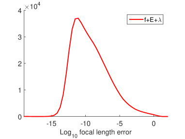
(a)	(b)

Figure 1: Numerical stability. (a) $\textrm{Log}_{10}$ of the relative error of the estimated radial distortion. (b) $\textrm{Log}_{10}$ of the relative error of the estimated focal length.

Numerical stability.

We studied the behavior of our solver on noise-free data. Figure 1(a) shows the experimental frequency of the base 10 logarithm of the relative error of the radial distortion parameter $\lambda$ estimated using the new f+E+$\lambda$ solver. These result were obtained by selecting the real roots closest to the ground truth values. The results suggest that the solver delivers correct solutions and its numerical stability is suitable for real word applications.

Figure 1(b) shows the distribution of $\textrm{Log}_{10}$ of the relative error of the estimated focal length $f$. Again these result were obtained by selecting the real roots closest to the ground truth values. Note that the f+E+$\lambda$ solver does not directly compute the focal length $f$. Its output is the monomial vector in $m$ (42), from which we extract $\lambda$ and the fundamental matrix $F=(x_{ij})$. To obtain the unknown focal length from $F$, we use the following formula:

Lemma 5.1.

Let $X=(x_{ij})_{1\leq i,j\leq 3}$ be a generic point in the variety $G^{\prime\prime}$ from Example 2.5. Then there are exactly two pairs of essential matrix and focal length $(E,f)$ such that $X=\textup{diag}(f^{-1},f^{-1},1)E$. If one of them is $(E,f)$ then the other is $(\textup{diag}(-1,-1,1)E,\,-f)$. In particular, f is determined up to sign by $X$. A formula to recover $f$ from $X$ is as follows:

$$f^{2}\,\,=\,\,\frac{x_{23}x_{31}^{2}+x_{23}x_{32}^{2}-2x_{21}x_{31}x_{33}-2x_{22}x_{32}x_{33}-x_{23}x_{33}^{2}}{2x_{11}x_{13}x_{21}+2x_{12}x_{13}x_{22}-x_{11}^{2}x_{23}-x_{12}^{2}x_{23}+x_{13}^{2}x_{23}+x_{21}^{2}x_{23}+x_{22}^{2}x_{23}+x_{23}^{3}}.$$ (43)

Proof.

Consider the map $E\times\mathbb{C}^{*}\rightarrow\mathbb{P}^{8}$, $(E,f)\mapsto\textup{diag}(f^{-1},f^{-1},1)E$. Let $I\subset\mathbb{Q}[e_{ij},f,x_{ij}]$ be the ideal of the graph of this map. So, $I$ is generated by the ten Demazure cubics and the nine entries of $X-\textup{diag}(f^{-1},f^{-1},1)E$. We computed the elimination ideal $I\cap\mathbb{Q}[f,x_{ij}]$ in Macaulay2. The polynomial gotten by clearing the denominator and subtracting the RHS from the LHS in the formula (43) lies in this elimination ideal. This proves the lemma. ∎

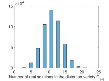
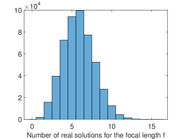
(a)	(b)

Figure 2: Number of real solutions for floating point computation with noise-free image data.

Counting real solutions.

In the next experiment we studied the distribution of the number of real solutions $(\lambda,F)$ and the number of real solutions for the focal length $f$.

Figure 2 (a) shows the histogram of the number of real solutions on the distortion variety $G^{\prime\prime}_{[v]}$. All odd integers between $1$ and $23$ were observed. Most of the time we got an odd number of real solutions between $7$ and $15$. The empirical probabilities are in Table 5.

real roots
in $G^{\prime\prime}_{[v]}$	1	3	5	7	9	11	13	15	17	19	21	23
$\%$	0.003	0.276	2.47	9.50	21.0	28.0	22.8	11.5	3.60	0.681	0.078	0.003

Table 5: Percentage of the number of real solutions in the distortion variety $G^{\prime\prime}_{[v]}$.

Figure 2 (b) shows the histogram of the number of solutions for the focal length $f$, computed from the distortion variety $G^{\prime\prime}_{[v]}$ using the formula (43). Of the $46$ complex solutions, at most $23$ could be real and positive. The largest number of positive real solutions $f$ observed in in 500,000 runs was $16$. The empirical probabilities from this experiment are in Table 6.

real $f$	0	1	2	3	4	5	6	7	8	9	10	11
$\%$	0.003	0.397	3.16	7.93	14.5	18.8	19.9	15.5	10.5	5.54	2.52	0.894
real $f$	12	13	14	15	16
$\%$	0.295	0.075	0.023	0.005	0.001

Table 6: Percentage of the number of positive real roots for the focal length $f$.

We performed the same experiment with image measurements corrupted by Gaussian noise with the standard deviation set to 2 pixels. The distribution of the real roots in the distortion variety $G^{\prime\prime}_{[v]}$ was very similar to the distribution for noise-free data. The main difference between these result and those for noise-free data was in the number of real values for the focal length $f$. For a fundamental matrix corrupted by noise, the formula (43) results in no real solutions more often. See Tables 7 and 8 for the empirical probabilities.

real roots	1	3	5	7	9	11	13	15	17	19	21	23
$\%$	0.021	0.509	3.23	11.2	22.4	27.7	21.1	10.1	3.07	0.566	0.062	0.004

Table 7: Percentage of the number of real solutions in the distortion variety $G^{\prime\prime}_{[v]}$ for image measurements corrupted with Gaussian noise with $\sigma=2$ pixels.

real $f$	0	1	2	3	4	5	6	7	8	9	10	11
$\%$	0.243	1.30	4.92	10.2	16.1	19.0	18.5	13.7	8.79	4.33	1.96	0.689
real $f$	12	13	14	15	16
$\%$	0.217	0.048	0.015	0.002	0.001

Table 8: Percentage of the number of real roots for the focal length $f$ with data as in Table 7.

Finally, we performed the same experiments for a special camera motion. It is known [29, 33] that the focal length cannot be determined by the formula (43) from the fundamental matrix if the optical axes are parallel to each other, e.g. for a sideways motion of cameras. Therefore, we generated cameras undergoing “close-to-sideways motion”. To model this scenario, 100 points were again placed in a 3D cube $\left[-\textrm{10},\textrm{10}\right]^{\textrm{3}}$. Then 500,000 different camera pairs were generated such that both cameras were first pointed in the same direction (optical axes were intersecting at infinity) and then translated laterally. Next, a small amount of rotational noise of 0.01 degrees was introduced into the camera poses by right-multiplying the projection matrices by respective rotation matrices. This multiplication slightly rotated the optical axes of cameras (as not to intersect at infinity) as well as simultaneously displaced the camera centers.

The results for noise-free data are displayed in Tables 10 and 10. For this special close-to-sideways motion, the formula (43) provides up to $20$ real solutions for the focal length $f$.

real roots	1	3	5	7	9	11	13	15	17	19	21	23
$\%$	0.007	0.544	5.14	16.83	26.2	24.9	16.2	7.37	2.30	0.475	0.061	0.006

Table 9: Real solutions in the distortion variety $G^{\prime\prime}_{[v]}$ for the close-to-sideways motion scenario.

real $f$	0	1	2	3	4	5	6	7	8	9	10	11
$\%$	0.006	0.755	3.08	10.2	12.9	20.9	16.2	16.0	8.73	6.17	2.61	1.58
real $f$	12	13	14	15	16	17	18	19	20
$\%$	0.556	0.253	0.086	0.033	0.011	0.0044	0.0016	0.0012	0.0002

Table 10: Real solutions for the focal length $f$ in the close-to-sideways motion scenario.

Acknowledgement.
This project started at the Algebraic Vision workshop (May 2016) at the American Institute of Mathematics (AIM) in San Jose. We are grateful to the organizers, Sameer Agarwal, Max Lieblich and Rekha Thomas, for bringing us together. Joe Kileel and Bernd Sturmfels were supported by the US National Science Foundation (DMS-1419018). Zuzana Kukelova was supported by the Czech Science Foundation (GACR P103/12/G08). Part of this study was carried out while she worked for Microsoft Research, Cambridge, UK. Tomas Pajdla was supported by H2020-ICT-731970 LADIO.

Authors’ addresses:

Joe Kileel and Bernd Sturmfels, University of California, Berkeley, USA, {jkileel,bernd}@berkeley.edu

Zuzana Kukelova and Tomas Pajdla, Czech Technical University in Prague, {kukelova,pajdla}@cvut.cz

References

- [1] E. Arnold: Modular algorithms for computing Gröbner bases, Journal of Symbolic Computation 35 (2003) 403–419.
- [2] C. Bocci, E. Carlini and J. Kileel: Hadamard products of linear spaces, Journal of Algebra 448 (2016) 595–617.
- [3] M. Bujnak: Algebraic Solutions to Absolute Pose Problems, Doctoral Thesis, Czech Technical University in Prague, 2012.
- [4] M. Bujnak, Z. Kukelova, and T. Pajdla: 3D reconstruction from image collections with a single known focal length, IEEE International Conference on Computer Vision, pp. 351–358, 2009.
- [5] M. Bujnak, Z. Kukelova and T. Pajdla: Making Minimal Solvers Fast, CVPR 2012 - IEEE Computer Society Conference on Computer Vision and Pattern Recognition, IEEE Computer Society Press, 2012.
- [6] M. Byrod, Z. Kukelova, K. Josephson, T. Pajdla and K. Åström: Fast and robust numerical solutions to minimal problems for cameras with radial distortion, CVPR 2008 – IEEE conf. on Computer Vision and Pattern Recognition.
- [7] E. Cattani, M. A. Cueto, A. Dickenstein, S. Di Rocco and B. Sturmfels: Mixed discriminants, Mathematische Zeitschrift 274 (2013) 761–778.
- [8] D. Cox, J. Little and H. Schenck: Toric Varieties, Graduate Studies in Mathematics, 124. American Mathematical Society, Providence, RI, 2011.
- [9] J. Dalbec and B. Sturmfels: Introduction to Chow forms, Invariant Methods in Discrete and Computational Geometry (ed. N. White), 37–58, Springer, New York, 1995.
- [10] M. Demazure: Sur deux problèmes de reconstruction, Technical Report 882, INRIA, Rocquencourt, France, 1988.
- [11] S. Di Rocco: Linear toric fibrations, Combinatorial Algebraic Geometry, Lecture Notes in Mathematics, Vol 2108, Springer, Cham, 2014, pp. 119–147.
- [12] D. Eisenbud and J. Harris: On varieties of minimal degree (a centennial account), Algebraic Geometry, Bowdoin, 1985, Proc. Sympos. Pure Math. 46, Part 1, Amer. Math. Soc., Providence, RI, 1987, pp. 3–13.
- [13] J.-C. Faugère: A new efficient algorithm for computing Gröbner bases (F4), Journal of Pure and Applied Algebra 139 (1999) 61–88.
- [14] M. Fischler and R. Bolles: Random sample consensus: a paradigm for model fitting with applications to image analysis and automated cartography, Commun. ACM 24 (1981) 381–395.
- [15] A. Fitzgibbon: Simultaneous linear estimation of multiple view geometry and lens distortion, IEEE Conf. on Computer Vision and Pattern Recognition, vol. I, pp. 125-132, 2001.
- [16] G. Floystad, J. Kileel and G. Ottaviani: The Chow form of the essential variety in computer vision, arXiv:1604.04372.
- [17] I.M. Gel’fand, M.M. Kapranov and A.V. Zelevinsky: Discriminants, Resultants and Multidimensional Determinants, Birkhäuser, Boston, 1994.
- [18] D. Grayson and M. Stillman: Macaulay2, a software system for research in algebraic geometry, available at www.math.uiuc.edu/Macaulay2/.
- [19] J. Harris: Algebraic Geometry. A First Course, Graduate Texts in Mathematics, 133, Springer-Verlag, New York, 1992.
- [20] R. Hartley and A. Zisserman: Multiple View Geometry in Computer Vision, Cambridge University Press, 2nd ed., 2003.
- [21] A. Jensen: Gfan, a software system for Gröbner fans and tropical varieties, Available at http://home.imf.au.dk/jensen/software/gfan/gfan.html.
- [22] F. Jiang, Y. Kuang, J.E. Solem and K. Åström: A minimal solution to relative pose with unknown focal length and radial distortion, 12th Asian Conference on Computer Vision, (ACCV 2014), 2014.
- [23] M. Kapranov, B. Sturmfels and A. Zelevinski: Chow polytopes and general resultants, Duke Mathematical Journal 67 (1992) 189–218.
- [24] Y. Kuang, J.E. Solem, F. Kahl and K. Åström: Minimal solvers for relative pose with a single unknown radial distortion, IEEE Conference on Computer Vision and Pattern Recognition (CVPR), pp. 33–40, 2014.
- [25] Z. Kukelova, M. Bujnak and T. Pajdla: Automatic Generator of Minimal Problem Solvers, ECCV 2008 - European Conference on Computer Vision, Lecture Notes in Computer Science 5304, pp. 302–315, Springer 2008.
- [26] Z. Kukelova: Algebraic Methods in Computer Vision, Doctoral Thesis, Czech Technical University in Prague, 2013.
- [27] D. Maclagan and B. Sturmfels: Introduction to Tropical Geometry, Graduate Studies in Mathematics, Vol 161, American Mathematical Society, 2015.
- [28] B. Micusik and T. Pajdla: Structure from motion with wide circular field of view cameras, IEEE Transactions on Pattern Analysis and Machine Intelligence 28 (2006) 1135–1149.
- [29] G. Newsam, D. Q. Huynh, M. Brooks and H. P. Pan: Recovering unknown focal lengths in self-calibration: An essentially linear algorithm and degenerate configurations. In Int. Arch. Photogrammetry & Remote Sensing, vol. XXXI-B3, pp. 575–580, 1996.
- [30] D. Nister: An efficient solution to the five-point relative pose problem, IEEE Transactions on Pattern Analysis and Machine Intelligence 26 (2004) 756–€“770.
- [31] S. Petrović: On the universal Gröbner bases of varieties of minimal degree, Mathematical Research Letters 15 (2008) 1211–1221.
- [32] H. Stewenius, D. Nister, F. Kahl and F. Schaffalitzky: A minimal solution for relative pose with unknown focal length. CVPR 2005 – IEEE conf. on Computer Vision and Pattern Recognition.
- [33] P. Sturm: On focal length calibration from two views, CVPR 2001 - IEEE Computer Society Conference on Computer Vision and Pattern Recognition, IEEE Computer Society Press, 2001.
- [34] B. Sturmfels: Gröbner Bases and Convex Polytopes, American Mathematical Society, Univ. Lectures Series, No 8, Providence, Rhode Island, 1996.
- [35] B. Sturmfels: Solving Systems of Polynomial Equations, American Mathematical Society, CBMS Regional Conferences Series, No 97, Providence, Rhode Island, 2002.
- [36] C. Traverso: Gröbner trace algorithms, Symbolic and Algebraic Computation, Lecture Notes in Computer Science, Vol 358, pp. 125–138, Springer, 2005.