A phase transition in a Curie-Weiss system with binary interactions

Abstract

A single-sort continuum Curie-Weiss system of interacting particles is studied. The particles are placed in the space $\mathds{R}^{d}$ divided into congruent cubic cells. For a region $V\subset\mathds{R}^{d}$ consisting of $N\in\mathds{N}$ cells, every two particles contained in $V$ attract each other with intensity $J_{1}/N$. The particles contained in the same cell are subjected to binary repulsion with intensity $J_{2}>J_{1}$. For fixed values of the temperature, the interaction intensities, and the chemical potential the thermodynamic phase is defined as a probability measure on the space of occupation numbers of cells, determined by a condition typical of Curie-Weiss theories. It is proved that the half-plane $J_{1}\,\times\,$chemical potential contains phase coexistence points at which there exist two thermodynamic phases of the system. An equation of state for this system is obtained.

Key words: equation of state, phase coexistence, mean field

Abstract

Ó ðîáîòi äîñëiäæåíî îäíîêîìïîíåíòíó íåïåðåðâíó ñèñòåìó чàñòèíîê iç âçàєìîäiєþ Êþði-Âåéñà. Чàñòèíêè ïåðåáóâàþòü ó ïðîñòîði $\mathds{R}^{d}$, ïîäiëåíîìó íà îäèíàêîâi êóáiчíi êîìiðêè. Äëÿ îáëàñòi $V\subset\mathds{R}^{d}$, ùî ñêëàäàєòüñÿ ç $N\in\mathds{N}$ êîìiðîê, êîæíi äâi чàñòèíêè, ùî ìiñòÿòüñÿ â $V$, ïðèòÿãóþòü îäíà îäíó ç iíòåíñèâíiñòþ $J_{1}/N$. Чàñòèíêè, ùî ìiñòÿòüñÿ â îäíié êîìiðöi, ïîïàðíî âiäøòîâõóþòüñÿ ç iíòåíñèâíiñòþ $J_{2}>J_{1}$. Äëÿ ôiêñîâàíèõ çíàчåíü òåìïåðàòóðè, iíòåíñèâíîñòi âçàєìîäi¿ òà õiìiчíîãî ïîòåíöiàëó òåðìîäèíàìiчíà ôàçà âèçíàчàєòüñÿ ÿê ìiðà éìîâiðíîñòi íà ïðîñòîði çàéíÿòèõ чèñåë êîìiðîê, ùî âèçíàчàєòüñÿ óìîâîþ, òèïîâîþ äëÿ òåîðié Êþði-Âåéñà. Äîâåäåíî, ùî íàïiâïëîùèíà $J_{1}\,\times\,$õiìiчíèé ïîòåíöiàë ìiñòèòü òîчêè ôàçîâîãî ñïiâiñíóâàííÿ, ïðè ÿêèõ iñíóþòü äâi òåðìîäèíàìiчíi ôàçè ñèñòåìè. Îòðèìàíî ðiâíÿííÿ ñòàíó äëÿ öiє¿ ñèñòåìè.

Ключовi слова: ìîëåêóëÿðíå ïîëå, ðiâíÿííÿ ñòàíó, ñïiâiñíóâàííÿ ôàç

1 Introduction

The mathematical theory of phase transitions in continuum particle systems has much fewer results as compared to its counterpart dealing with discrete underlying sets like lattices, graphs, etc. It is then quite natural that the first steps in such theories are being made by employing various mean field models. In [1], the mean field approach was mathematically realized by using a Kac-like infinite range attraction combined with a two-body repulsion. By means of rigorous upper and lower bounds for the canonical partition function obtained in that paper, the authors derived the equation of state indicating the possibility of a first-order phase transition. Later on, this result was employed in [2, 3] to go beyond the mean field, see also [4, 5] for recent results. Another way of realizing the mean-field approach is to use Curie-Weiss interactions and then appropriate the methods of calculating the asymptotics of integrals, cf. [6]. Quite recently, this way was formulated as a coherent mathematical theory based on the large deviation techniques, in the framework of which the Gibbs states (thermodynamic phases) of the system are constructed as probability measures on an appropriate phase space, see [7, section II].

In this work, we introduce a simple Curie-Weiss type model of a single-sort continuum particle system in which the space $\mathds{R}^{d}$ is divided into congruent (cubic) cells. For a bounded region $V\subset\mathds{R}^{d}$ consisting of $N$ such cells, the attraction between every two particles in $V$ is set to be $J_{1}/N$, regardless of their positions. If such two particles lie in the same cell, they repel each other with intensity $J_{2}>J_{1}$. Unlike [1], we deal with the grand canonical ensemble. Therefore, our initial thermodynamic variables are the inverse temperature $\beta=1/k_{\text{B}}T$ and the physical chemical potential. However, for the sake of convenience we employ the variables $p=\beta J_{1}$ and $\mu=\beta\,\times\,$(physical chemical potential) and define single-phase domains of the half-plane $\{(p,\mu):p>0,\mu\in\mathds{R}\}$ (see definition 2.1) by a condition that ensures the existence of a unique $\bar{y}\in\mathds{R}$, which determines a probability measure $\mathbf{Q}_{p,\mu}$, given in (2.22) and (2.21). In the grand canonical formalism and in the approach of [7], this measure is set to be the thermodynamic phase of the system. The points $(p,\mu)$ where the mentioned single-phase condition fails to hold due to the existence of multiple $\bar{y}$ correspond to the coexistence of multiple thermodynamic phases. In theorem 2.1, we show that there exists $p_{0}>0$ such that $\mathcal{R}(p_{0}):=\{(p,\mu):p\in(0,p_{0}),\mu\in\mathds{R}\}$ is a single-phase domain, that is, there is no phase-coexistence point in the strip $\mathcal{R}(p_{0})$ for small enough attractions. Note that for some models on graphs, see the example given in [8], there exist multiple phases for each positive attraction. Thereafter, in theorem 2.2 we show that for each value of $J_{2}/J_{1}:=a>1$, there exist points in which two phases do coexist. Namely, we show that there exists $p_{1}>0$ such that for each $p\geqslant p_{1}$, there exists $\mu_{\text{c}}(p)\in\mathds{R}$ and small enough $\epsilon>0$ such that the sets $\{(p,\mu):\mu\in(\mu_{\text{c}}(p)-\epsilon,\mu_{\text{c}}(p))\}$ and $\{(p,\mu):\mu\in(\mu_{\text{c}}(p),\mu_{\text{c}}(p)+\epsilon)\}$ lie in different single-phase domains, and that there exist at least two $\bar{y}$ whenever $\mu=\mu_{\text{c}}(p)$. In section 3, we present a number of results of the corresponding numerical calculations which illustrate the postulates proved in theorems 2.1 and 2.2.

2 The model

By $\mathds{N}$, $\mathds{R}$ and $\mathds{C}$ we denote the sets of natural, real and complex numbers, respectively. We also put $\mathds{N}_{0}=\mathds{N}\cup\{0\}$. For $d\in\mathds{N}$, by $\mathds{R}^{d}$, we denote the Euclidean space of vectors $x=(x^{1},\dots,x^{d})$, $x^{i}\in\mathds{R}$. In the sequel, its dimension $d$ will be fixed. By $dx$ we mean the Lebesgue measure on $\mathds{R}^{d}$. In this section, we use some tools of the analysis on configuration spaces whose main aspects can be found in [9].

2.1 The integration

For $n\in\mathds{N}$, let $\Gamma^{(n)}$ be the set of all $n$-point subsets of $\mathds{R}^{d}$. Every subset of this kind, $\gamma\in\Gamma^{(n)}$ (called configuration), is an $n$-element set of distinct points $x\in\mathds{R}^{d}$. Let also $\Gamma^{(0)}$ be the one–element set consisting of the empty configuration. Every $\Gamma^{(n)}$ is equipped with the topology related to the Euclidean topology of $\mathds{R}^{d}$. Then, we define

$$\Gamma_{0}=\bigsqcup_{n\in\mathds{N}_{0}}\Gamma^{(n)},$$

that is, $\Gamma_{0}$ is the topological sum of the spaces $\Gamma^{(n)}$. We equip $\Gamma_{0}$ with the corresponding Borel $\sigma$-field $\mathcal{B}(\Gamma_{0})$ that makes $(\Gamma_{0},\mathcal{B}(\Gamma_{0}))$ a standard Borel space. A function $G:\Gamma_{0}\to\mathds{R}$ is $\mathcal{B}(\Gamma_{0})$-measurable if and only if, for each $n\in\mathds{N}$, there exists a symmetric Borel function $G^{(n)}:(\mathds{R}^{d})^{n}\to\mathds{R}$ such that $G(\gamma)=G^{(n)}(x_{1},\dots,x_{n})$ for $\gamma=\{x_{1},\dots,x_{n}\}$. For such a function $G$, we also set $G^{(0)}=G(\varnothing)$. The Lebesgue-Poisson measure $\lambda$ on $(\Gamma_{0},\mathcal{B}(\Gamma_{0}))$ is defined by the relation

$$\int_{\Gamma_{0}}G(\gamma)\lambda(\mathrm{d}\gamma)=G^{(0)}+\sum_{n=1}^{\infty}\frac{1}{n!}\int_{(\mathds{R}^{d})^{n}}G^{(n)}(x_{1},\dots,x_{n})\mathrm{d}x_{1}\dots\mathrm{d}x_{n}\,,$$ (2.1)

which should hold for all measurable $G:\Gamma_{0}\to\mathds{R}_{+}:=[0,+\infty)$ for which the right-hand side of (2.1) is finite.

For some $c>0$, we let $\Delta=(-c/2,c/2]^{d}\subset\mathds{R}^{d}$ be a cubic cell of volume $\upsilon=c^{d}$ centered at the origin. Let also $V\subset\mathds{R}^{d}$ be the union of $N\in\mathds{N}$ disjoint translates $\Delta_{\ell}$ of $\Delta$, i.e.,

$$V=\bigcup_{\ell=1}^{N}\Delta_{\ell}.$$

As is usual for Curie-Weiss theories, cf. [6, 7], the form of the interaction energy of the system of particles placed in $V$ depends on $V$. In our model, the energy of a configuration $\gamma\subset V$ is

$$W_{N}(\gamma) = \frac{1}{2}\sum_{x,y\in\gamma}\Phi_{N}(x,y),$$

$$\Phi_{N}(x,y) = -J_{1}/N+J_{2}\sum_{\ell=1}^{N}\mathds{I}_{\Delta_{\ell}}(x)\mathds{I}_{\Delta_{\ell}}(y),$$ (2.2)

where $\mathds{I}_{\Delta_{\ell}}$ is the indicator of $\Delta_{\ell}$, that is, $\mathds{I}_{\Delta_{\ell}}(x)=1$ if $x\in\Delta_{\ell}$ and $\mathds{I}_{\Delta_{\ell}}(x)=0$ otherwise. For convenience, in $W_{N}$ above we have included the self-interaction term $\Phi_{N}(x,x)$, which does not affect the physics of the model. We also write $W_{N}$ and $\Phi_{N}$ instead of $W_{V}$ and $\Phi_{V}$ since these quantities depend only on the number of cells in $V$. The first term in $\Phi_{N}$ with $J_{1}>0$ describes the attraction. By virtue of the Curie-Weiss approach, it is taken equal for all particles. The second term with $J_{2}>0$ describes the repulsion between two particles contained in one and the same cell. That is, in our model every two particles in $V$ attract one another independently of their location, and repel if they are in the same cell. The intensities $J_{1}$ and $J_{2}$ are assumed to satisfy the following condition

$$J_{2}>J_{1}.$$ (2.3)

The latter is to secure the stability of the interaction [10], that is, to satisfy

$$\int_{V}\Phi_{N}(x,y)\mathrm{d}y>0,\qquad{\rm for}\ {\rm all}\ x\in V.$$

Let $\beta=1/k_{\rm B}T$ be the inverse temperature. To optimize the choice of the thermodynamic variables we introduce the following ones

$$p=\beta J_{1}\,,\qquad a=J_{2}/J_{1}\,,$$ (2.4)

and the dimensionless chemical potential $\mu=\beta\,\times\,$(physical chemical potential). Then, $(p,\mu)\in\mathds{R}_{+}\times\mathds{R}$ is considered to be the basic set of thermodynamic variables, whereas $a$ and $\upsilon$ are model parameters.

The grand canonical partition function in region $V$ is

$$\Xi_{N}(p,\mu) = \int_{\Gamma_{V}}\exp\left[\mu|\gamma|-\beta W_{N}(\gamma)\right]\lambda(\mathrm{d}\gamma)$$ (2.5)

$$= \int_{\Gamma_{V}}\exp\left[\mu|\gamma|+\frac{p}{2N}|\gamma|^{2}-\frac{ap}{2}\sum_{x,y\in\gamma}\sum_{\ell=1}^{N}\mathds{I}_{\Delta_{\ell}}(x)\mathds{I}_{\Delta_{\ell}}(y)\right]\lambda(\mathrm{d}\gamma),$$

where $|\gamma|$ stands for the number of points in the configuration $\gamma$, and $\Gamma_{V}$ is the subset of $\Gamma_{0}$ consisting of all $\gamma$ contained in $V$. We write $\Xi_{N}$ instead of $\Xi_{V}$ for the reasons mentioned above.

2.2 Transforming the partition function

Now we use a concrete form of the energy as in (2.1) to bring (2.5) to a more convenient form. For a given $\ell=1,\dots,N$ and a configuration $\gamma\in\Gamma_{V}$, we set $\gamma_{\ell}=\gamma\cap\Delta_{\ell}$, that is, $\gamma_{\ell}$ is the part of the configuration contained in $\Delta_{\ell}$. Then, $|\gamma_{\ell}|$ will stand for the number of points of $\gamma$ contained in $\Delta_{\ell}$. Note that

$$|\gamma_{\ell}|=\sum_{x\in\gamma_{\ell}}1=\sum_{x\in\gamma}\mathds{I}_{\Delta_{\ell}}(x).$$ (2.6)

Then, cf. (2.1) and (2.5),

$$\sum_{x,y\in\gamma}\Phi_{N}(x,y)=\sum_{\ell,\ell^{\prime}=1}^{N}\sum_{x\in\Delta_{\ell}}\sum_{y\in\Delta_{\ell^{\prime}}}\Phi_{N}(x,y)=-\frac{J_{1}}{N}\left(\sum_{\ell=1}^{N}|\gamma_{\ell}|\right)^{2}+J_{2}\sum_{\ell=1}^{N}\left|\gamma_{\ell}\right|^{2}.$$

To rewrite the integrand in (2.5) in a more convenient form we set

$$F_{N}(\varrho,p,\mu)=\exp\left[\frac{p}{2N}\left(\sum_{\ell=1}^{N}\varrho_{\ell}\right)^{2}+\mu\sum_{\ell=1}^{N}\varrho_{\ell}-\frac{ap}{2}\sum_{\ell=1}^{N}\varrho_{\ell}^{2}\right],$$ (2.7)

where $\varrho\in\mathds{N}_{0}^{N}$ is a vector with nonnegative integer components $\varrho_{\ell}$, $\ell=1,2,\dots,N$. Then, (2.5) takes the form

$$\Xi_{N}(p,\mu)=\int_{\Gamma_{V}}F_{N}\big{(}\nu(\gamma),p,\mu\big{)}\lambda(\mathrm{d}\gamma),$$ (2.8)

where $F_{N}$ is as in (2.7) and $\nu(\gamma)\in\mathds{N}_{0}^{N}$ is the vector with component $|\gamma_{\ell}|$, $\ell=1,\dots,N$. For $n,m\in\mathds{N}_{0}$, the Kronecker $\delta$-symbol can be written

$$\delta_{nm}=\int_{0}^{1}\exp\left[2\piup{\rm i}t(n-m)\right]\mathrm{d}t,\qquad{\rm i}=\sqrt{-1}.$$

Applying this in (2.8) we get

$$\Xi_{N}(p,\mu) = \sum_{\varrho\in\mathds{N}_{0}^{N}}F_{N}(\varrho,p,\mu)\int_{\Gamma_{V}}\int_{[0,1]^{N}}\exp\left[2\piup{\rm i}\sum_{\ell=1}^{N}\left(\varrho_{\ell}-|\gamma_{\ell}|\right)t_{\ell}\right]\lambda(\mathrm{d}\gamma)\mathrm{d}t_{1}\dots\mathrm{d}t_{N}$$ (2.9)

$$= \sum_{\varrho\in\mathds{N}_{0}^{N}}F_{N}(\varrho,p,\mu)\int_{[0,1]^{N}}\exp\bigg{(}2\piup{\rm i}\sum_{\ell=1}^{N}\varrho_{\ell}t_{\ell}\bigg{)}R_{N}(t_{1},\dots,t_{N})\mathrm{d}t_{1}\dots\mathrm{d}t_{N}.$$

Here,

$$R_{N}(t_{1},\dots,t_{N}) = \int_{\Gamma_{V}}\exp\bigg{(}-2\piup{\rm i}\sum_{\ell=1}^{N}|\gamma_{\ell}|t_{\ell}\bigg{)}\lambda(\mathrm{d}\gamma)=\int_{\Gamma_{V}}\exp\bigg{[}-2\piup{\rm i}\sum_{\ell=1}^{N}\sum_{x\in\gamma}\mathds{I}_{\Delta_{\ell}}(x)t_{\ell}\bigg{]}\lambda(\mathrm{d}\gamma)$$ (2.10)

$$= \sum_{n=0}^{\infty}\frac{1}{n!}\int_{V^{n}}\exp\bigg{[}-2\piup{\rm i}\sum_{\ell=1}^{N}\sum_{j=1}^{n}\mathds{I}_{\Delta_{\ell}}(x_{j})t_{\ell}\bigg{]}\mathrm{d}x_{1}\dots\mathrm{d}x_{n}.$$

In getting the second line of (2.10), we use (2.6), and then the integral with $\lambda$ is written according to (2.1). Note that the expression under the integral in the last line of (2.10) factors in $j$, which allows for writing it in the form

$$R_{N}(t_{1},\dots,t_{N}) = \sum_{n=0}^{\infty}\frac{1}{n!}\left\{\int_{V}\exp\left[-2\piup{\rm i}\sum_{\ell=1}^{N}\mathds{I}_{\Delta_{\ell}}(x)t_{\ell}\right]\mathrm{d}x\right\}^{n}$$

$$= \sum_{n=0}^{\infty}\frac{1}{n!}\left[\sum_{\ell=1}^{N}\int_{\Delta_{\ell}}\exp\left(-2\piup{\rm i}t_{\ell}\right)\mathrm{d}x\right]^{n}=\exp\left[\upsilon\sum_{\ell=1}^{N}\exp\left(-2\piup{\rm i}t_{\ell}\right)\right].$$

Now we apply this in (2.9) and obtain

$$\Xi_{N}(p,\mu)=\sum_{\varrho\in\mathds{N}_{0}^{N}}F_{N}(\varrho,p,\mu)\prod_{\ell=1}^{N}\left(\frac{\upsilon^{\varrho_{\ell}}}{\varrho_{\ell}!}\right)=\sum_{\varrho\in\mathds{N}_{0}^{N}}\exp\left[\frac{p}{2N}\left(\sum_{\ell=1}^{N}\varrho_{\ell}\right)^{2}\right]\prod_{\ell=1}^{N}\pi(\varrho_{\ell},\mu),$$ (2.11)

where $p$ is as in (2.4) and

$$\pi(n,\mu)=\frac{\upsilon^{n}}{n!}\exp\left(\mu n-\frac{1}{2}apn^{2}\right),\qquad n\in\mathds{N}_{0}.$$ (2.12)

Note that, for $p=0,\pi$ turns into the (non-normalized) Poisson distribution with parameter $\upsilon\mathrm{e}^{\,\mu}$. Hence, alternating the cell size amounts to shifting $\mu$.

2.3 Single-phase domains

By a standard identity

$$\exp\left[\frac{p}{2N}\left(\sum_{\ell=1}^{N}\varrho_{\ell}\right)^{2}\right]=\sqrt{\frac{N}{2\piup p}}\int_{\mathds{R}}\exp\Bigg{(}-N\frac{y^{2}}{2p}+y\sum_{\ell=1}^{N}\varrho_{\ell}\Bigg{)}\mathrm{d}y,$$

we transform (2.11) into the following expression

$$\Xi_{N}(p,\mu)=\sqrt{\frac{N}{2\piup p}}\int_{\mathds{R}}\exp\left[NE(y,p,\mu)\right]\mathrm{d}y,$$ (2.13)

where

$$E(y,p,\mu)=-\frac{y^{2}}{2p}+\ln K(y,p,\mu),$$ (2.14)

and, cf. (2.4) and (2.12),

$$K(y,p,\mu)=\sum_{n=0}^{\infty}\frac{\upsilon^{n}}{n!}\exp\left[(y+\mu)n-\frac{ap}{2}n^{2}\right].$$ (2.15)

Note that $E$ is an infinitely differentiable function of all its arguments. Set

$$P_{N}(p,\mu)=\frac{1}{\upsilon N}\ln\Xi_{N}(p,\mu).$$ (2.16)

By the following evident inequality

$$(y+\mu)n-\frac{ap}{2}n^{2}\leqslant\frac{(y+\mu)^{2}}{2ap}\,,\qquad n\in\mathds{N}_{0}\,,$$

we obtain from (2.15) and (2.14) that

$$E(y,p,\mu)\leqslant-\frac{a-1}{2ap}y^{2}+\frac{\mu}{2ap}(2y+\mu)+\upsilon.$$ (2.17)

By virtue of Laplace’s method [11], to calculate the large $N$ limit in (2.16) we should find the global maxima of $E(y,p,\mu)$ as a function of $y\in\mathds{R}$.

Remark 2.1.

From the estimate in (2.17) it follows that: (a) the integral in (2.13) is convergent for all $p>0$ and $\mu\in\mathds{R}$ since $a>1$, see (2.3) and (2.4); (b) for fixed $p$ and $\mu$, as the bounded from the above function $E(y,p,\mu)$ has global maxima, each of which is also its local maximum.

To get (b) we observe that (2.17) implies $\lim_{|y|\to+\infty}E(y,p,\mu)=-\infty$; hence, each point $\bar{y}$ of global maximum belongs to a certain interval $(\bar{y}-\varepsilon,\bar{y}+\varepsilon)$, where it is also a maximum point. Since $E$ is everywhere differentiable in $y$, then $\bar{y}$ is the point of global maximum only if it solves the following equation

$$E_{1}(y,p,\mu):=\frac{\partial}{\partial y}E(y,p,\mu)=0.$$ (2.18)

By (2.14) and (2.15) this equation can be rewritten in the form

$$-\frac{y}{p}+\frac{K_{1}(y,p,\mu)}{K(y,p,\mu)}=0,$$

$$K_{1}(y,p,\mu):=\sum_{n=1}^{\infty}\frac{n\upsilon^{n}}{n!}\exp\left[(y+\mu)n-\frac{ap}{2}n^{2}\right].$$

Remark 2.2.

As we will see from the proof of theorem 2.1 below, the equation in (2.3) has at least one solution for all $p>0$ and $\mu\in\mathds{R}$. Since both $K_{1}$ and $K$ take only strictly positive values, these solutions are also strictly positive.

Definition 2.1.

We say that $(p,\mu)$ belongs to a single-phase domain if $E(y,p,\mu)$ has a unique global maximum $\bar{y}\in\mathds{R}$ such that

$$E_{2}(\bar{y},p,\mu):=\frac{\partial^{2}}{\partial y^{2}}E(y,p,\mu)\Big{|}_{y=\bar{y}}<0.$$ (2.20)

Note that $\bar{y}$ can be a point of maximum if $E_{1}(\bar{y},p,\mu)=E_{2}(\bar{y},p,\mu)=0$. That is, not every point of global maximum corresponds to a point in a single-phase domain.

The condition in (2.3) determines the unique probability measure $Q_{p,\mu}$ on $\mathds{N}_{0}$ such that

$$Q_{p,\mu}(n)=\frac{1}{K(\bar{y},p,\mu)n!}\upsilon^{n}\exp\left[(\bar{y}+\mu)n-\frac{ap}{2}n^{2}\right],\qquad n\in\mathds{N}_{0}\,,$$ (2.21)

which yields the probability law of the occupation number of a single cell. Then, the unique thermodynamic phase of the model corresponding to $(p,\mu)\in\mathcal{R}$ is the product

$$\mathbf{Q}_{p,\mu}=\bigotimes_{\ell=1}^{\infty}Q^{(\ell)}_{p,\mu}$$ (2.22)

of the copies of the measure defined in (2.21). It is a probability measure on the space of all vectors $\mathbf{n}=(n_{\ell})_{\ell=1}^{\infty}$, in which $n_{\ell}\in\mathds{N}_{0}$ is the occupation number of $\ell$-th cell.

The role of the condition in (2.20) is to yield the possibility to apply Laplace’s method for asymptotic calculation of the integral in (2.13). By direct calculations, it follows that

$$E_{2}(y,p,\mu)=-\frac{1}{p}+\frac{1}{2\left[K(y,p,\mu)\right]^{2}}$$ (2.23)

$$\quad\times\sum_{n_{1},n_{2}=0}^{\infty}\frac{\upsilon^{n_{1}+n_{2}}}{n_{1}!n_{2}!}(n_{1}-n_{2})^{2}\exp\left[(y+\mu)(n_{1}+n_{2})-\frac{ap}{2}(n_{1}^{2}+n_{2}^{2})\right].$$

In dealing with the equation in (2.3) we fix $p>0$ and consider $E_{1}$ as a function of $y\in\mathds{R}$ and $\mu\in\mathds{R}$. Then, for a given $\mu_{0}$, we solve (2.3) to find $\bar{y}_{0}$ and then check whether it is the unique point of global maximum and (2.20) is satisfied, i.e., whether $(p,\mu_{0})$ belongs to a single-phase domain. Then, we slightly vary $\mu$ and repeat the same. This will yield a function $\mu\mapsto\bar{y}(\mu)$ defined in the neighbourhood of $\mu_{0}$, which dependends on the choice of $p$ and satisfies $\bar{y}(\mu_{0})=\bar{y}_{0}$. In doing so, we use the analytic implicit function theorem based on the fact that, for each fixed $p>0$, the function $\mathds{R}^{2}\ni(y,\mu)\mapsto E_{1}(y,p,\mu)$ can be analytically continued to some complex neighbourhood of $\mathds{R}^{2}$, see (2.15) and (2.3). For the reader’s convenience, we present this theorem here in the form adapted from [12, section 7.6, page 34]. For some $p_{0}>0$, let $\mathcal{B}\subset\mathds{C}^{2}$ be a connected open set containing $\mathds{R}^{2}$ such that the function $(y,\mu)\mapsto E_{1}(y,p_{0},\mu)$ should be analytic in $\mathcal{B}$.

Proposition 2.1 (Implicit function theorem).

Let $p_{0}$ and $(y_{0},\mu_{0})$ be such that $E_{1}(y_{0},p_{0},\mu_{0})=0$ and $E_{2}(y_{0},p_{0},\mu_{0})\neq 0$. Let also $\mathcal{B}\subset\mathds{C}^{2}$ be as just described. Then, there exist open sets $\mathcal{D}_{1}\subset\mathds{C}$ and $\mathcal{D}_{2}\subset\mathds{C}$ such that $y_{0}\in\mathcal{D}_{1}$, $\mu_{0}\in\mathcal{D}_{2}$, $\mathcal{D}_{1}\times\mathcal{D}_{2}\subset\mathcal{B}$, and an analytic function $\bar{y}:\mathcal{D}_{2}\to\mathcal{D}_{1}$, for which the following holds

$$\{(y,\mu)\in\mathcal{D}_{1}\times\mathcal{D}_{2}:E_{1}(y,p_{0},\mu)=0\}=\{(\bar{y}(\mu),\mu):\mu\in\mathcal{D}_{2}\}.$$

The derivative of $\bar{y}$ in $\mathcal{D}_{2}$ is

$$\frac{\mathrm{d}\bar{y}(\mu)}{\mathrm{d}\mu}=-\frac{1}{E_{2}(\bar{y}(\mu),p_{0},\mu)}\left[\frac{\partial}{\partial\mu}E_{1}(y,p_{0},\mu)\right]_{y=\bar{y}(\mu)}.$$ (2.24)

Remark 2.3.

In the sequel, we also use the version of the implicit function theorem in which we do not employ the analytic continuation of $E_{1}$ to complex values of $p$. Let the conditions of proposition 2.1 regarding $E_{1}$ and $E_{2}$ be satisfied. Then, there exist open sets $\mathcal{D}_{i}\subset\mathds{R}$, $i=1,2,3$, and a continuous function $\bar{y}:\mathcal{D}_{3}\times\mathcal{D}_{2}\to\mathcal{D}_{1}$ such that $p_{0}\in\mathcal{D}_{3}$, $\mu_{0}\in\mathcal{D}_{2}$ and the following holds

$$\{(y,p,\mu)\in\mathcal{D}_{1}\times\mathcal{D}_{2}\times\mathcal{D}_{3}:E_{1}(y,p_{0},\mu)=0\}=\{(\bar{y}(p,\mu),p,\mu):p\in\mathcal{D}_{3},\ \mu\in\mathcal{D}_{2}\}.$$

The partial derivative of $\bar{y}(p,\mu)$ over $\mu\in\mathcal{D}_{2}$ is given by the right-hand side of (2.24). In the sequel, by writing $\bar{y}(\mu)$ we assume both the function as proposition 2.1, defined for a fixed $p$ known from the context, and that as in remark 2.3 with the fixed value of $p$.

For a fixed $p_{0}>0$, assume that $(p_{0},\mu_{0})$ belongs to a single-phase domain. By proposition 2.1 there exists $\varepsilon>0$ such that the function $(\mu_{0}-\varepsilon,\mu_{0}+\varepsilon)\ni\mu\mapsto\bar{y}(\mu)$ can be defined by the equation $E_{1}(y,p_{0},\mu)=0$. Its continuation from the mentioned interval is related to the fulfilment of the condition $E_{2}(\bar{y}(\mu),p_{0},\mu)<0$, cf. (2.20), which may not be the case. At the same time, by (2.23) we have that

$$\frac{\partial}{\partial\mu}E_{1}(y,p,\mu)=E_{2}(y,p,\mu)+\frac{1}{p}>0,$$

holding for all $y\in\mathds{R}$, $p>0$ and $\mu\in\mathds{R}$. In view of this and (2.24), it might be more convenient to use the inverse function $y\mapsto\bar{\mu}(y)$ since the $\mu$-derivative of $E_{1}$ is always nonzero. Its properties are described by the following statement obtained from the analytic implicit function theorem mentioned above. Recall that only positive $y$ solves the equation in (2.3).

Proposition 2.2.

Given $p_{0}$, let $\mathcal{B}$ be as in proposition 2.1. Then, there exist open connected subsets $\mathcal{D}_{i}\subset\mathds{C}$, $i=1,2$, and an analytic function $\mathcal{D}_{1}\ni y\mapsto\bar{\mu}(y)\in\mathcal{D}_{2}$ such that $\mathcal{D}_{1}$ contains $\mathds{R}_{+}$, $\mathcal{D}_{1}\times\mathcal{D}_{2}\subset\mathcal{B}$, and the following holds

$$\{(y,\mu)\in\mathcal{D}_{1}\times\mathcal{D}_{2}:E_{1}(y,p_{0},\mu)=0\}=\{(y,\bar{\mu}(y)):y\in\mathcal{D}_{1}\}.$$

The derivative of $\bar{\mu}$ in $\mathcal{D}_{1}$ is

$$\frac{\mathrm{d}\bar{\mu}(y)}{\mathrm{d}y}=-\frac{E_{2}(y,p_{0},\bar{\mu}(y))}{E_{2}(y,p_{0},\bar{\mu}(y))+\frac{1}{p}}.$$

Proposition 2.3.

Each single-phase domain, $\mathcal{R}$, has the following properties: (a) it is an open subset of $\mathds{R}_{+}\times\mathds{R}$; (b) for each $(p_{0},\mu_{0})\in\mathcal{R}$, the function $\mathcal{I}_{p_{0}}:=\{\mu\in\mathds{R}:(p_{0},\mu)\in\mathcal{R}\}\ni\mu\mapsto\bar{y}(\mu)$ as in proposition 2.1 is continuously differentiable on $\mathcal{I}_{p_{0}}$. Moreover,

$$\frac{\mathrm{d}\bar{y}(\mu)}{\mathrm{d}\mu}>0,\qquad{\textit{f}or}\ {\textit{a}ll}\ \mu\in\mathcal{I}_{p_{0}}.$$ (2.25)

Proof.

For a single-phase domain, $\mathcal{R}$, take $(p_{0},\mu_{0})\in\mathcal{R}$. By remark 2.3 the function $(p,\mu)\mapsto\bar{y}(p,\mu)$, defined by the equation $E_{1}(y,p,\mu)=0$ is continuous in some open subset of $\mathcal{R}$ containing $(p_{0},\mu_{0})$. By the continuity of $E_{2}(\bar{y}(p,\mu),p,\mu)$ and the fact that $E_{2}(\bar{y}(p_{0},\mu_{0}),p_{0},\mu_{0})<0$ (since $(p_{0},\mu_{0})\in\mathcal{R}$) we get that $E_{2}(\bar{y}(p,\mu),p,\mu)<0$ for $(p,\mu)$ in some open neighbourhood of $(p_{0},\mu_{0})$. Hence, $\mathcal{R}$ contains $(p_{0},\mu_{0})$ with some neighbourhood and thus is open. The continuous differentiability of $\bar{y}$ and the sign rule in (2.25) follow by proposition 2.1 and (2.24), respectively. ∎

By (2.21) and (2.3) we get the $Q_{p,\mu}$-mean value $\bar{n}=\bar{n}(p,\mu)$ of the occupation number of a given cell in the form

$$\bar{n}(p,\mu)=\sum_{n=0}^{\infty}nQ_{p,\mu}(n)=\frac{K_{1}(\bar{y}(p,\mu),p,\mu)}{K(\bar{y}(p,\mu),p,\mu)}=\frac{\bar{y}(p,\mu)}{p}.$$ (2.26)

Note that, up to the factor $\upsilon^{-1}$, $\bar{n}(p,\mu)$ is the particle density in phase $\mathbf{Q}_{p,\mu}$. For a fixed $p$, by proposition 2.3 $\bar{n}(p,\cdot)$ in an increasing function on $\mathcal{I}_{p}$, which can be inverted to give $\bar{\mu}(p,\bar{n})$. By Laplace’s method we then get the following corollary of proposition 2.3.

Proposition 2.4.

Let $\mathcal{R}$ be a single-phase domain. Then, for each $(p,\mu)\in\mathcal{R}$, the limiting pressure $P(p,\mu)=\lim_{N\to+\infty}P_{N}(p,\mu)$, see (2.16), exists and is continuously differentiable on $\mathcal{R}$. Moreover, it is given by the following formula

$$P(p,\mu)=\upsilon^{-1}E(\bar{y}(p,\mu),p,\mu).$$ (2.27)

Let $\mathcal{N}_{p}$ be the image of $\mathcal{I}_{p}$ under the map $\mu\mapsto\bar{n}(p,\mu)$. Then, the inverse map $\bar{n}\mapsto\bar{\mu}(p,\bar{n})$ is continuously differential and increasing on $\mathcal{N}_{p}$. By means of this map, for a fixed $p$, the pressure given in (2.27) can be written as a function of $\bar{n}$

$$P=\bar{P}(\bar{n})=\upsilon^{-1}E(p\bar{n},p,\bar{\mu}(p,\bar{n})),\qquad\bar{n}\in\mathcal{N}_{p}\,,$$ (2.28)

which is the equation of state.

2.4 The phase transition

Recall that the notion of the single-phase domain was introduced in definition 2.1, and each domain of this kind is an open subset of the open right half-plane $\{(p,\mu):p>0,\ \mu\in\mathds{R}\}$, see proposition 2.3. With this regard we have the following possibilities: (i) the whole half-plane $\{(p,\mu):p>0,\ \mu\in\mathds{R}\}$ is such a domain; (ii) there exist more than one single-phase domain. In case (i), for all $(p,\mu)$ there exists one phase (2.22). In the context of this work, a phase transition is understood as the possibility of having different phases at the same value of the pair $(p,\mu)$. If this is the case, $(p,\mu)$ is called a phase coexistence point. Clearly, such a point should belong to the common topological boundary of at least two distinct single-phase domains. That is, to prove the existence of phase transitions we have to show that possibility (ii) takes place and that these single-phase domains have a common boundary. We do this in theorems 2.1 and 2.2 below.

Let $\mathcal{R}$ be a single-phase domain. Take $(p_{0},\mu_{0})\in\mathcal{R}$ and consider the line $l_{p_{0}}=\{(p_{0},\mu):\mu\in\mathds{R}\}$. If the whole line lies in $\mathcal{R}$, by proposition 2.3, $\bar{y}(\mu)$ is a continuously differentiable and increasing function of $\mu\in\mathds{R}$. In our first theorem, we prove that this is the case for small enough $p_{0}$.

Theorem 2.1.

There exists $p_{0}>0$ such that the set $\mathcal{R}(p_{0}):=\{(p,\mu):p\in(0,p_{0}]\}$ is a single-phase domain.

Proof.

In view of remark 2.1, we have to show that, for fixed $p\leqslant p_{0}$ and all $\mu\in\mathds{R}$, $E(y,p,\mu)$ has exactly one local maximum such that (2.20) holds. For $x\in\mathds{R}$, we set, cf. (2.15),

$$\phi(x,p) = \ln\sum_{n=0}^{\infty}\frac{\upsilon^{n}}{n!}\exp\left(xn-\frac{ap}{2}n^{2}\right),$$ (2.29)

$$\phi_{k}(x,p) = \frac{\partial^{k}}{\partial x^{k}}\phi(x,p),\qquad k=1,2.$$

Similarly to (2.17), we get

$$\phi(x,p)\leqslant\upsilon+\frac{x^{2}}{2ap}\,.$$ (2.30)

Note also that, for the functions defined in (2.29), we have

$$\lim_{p\to 0}\phi(x,p)=\lim_{p\to 0}\phi_{1}(x,p)=\lim_{p\to 0}\phi_{2}(x,p)=\upsilon\mathrm{e}^{x},\qquad x\in\mathds{R}.$$ (2.31)

By means of (2.29) we rewrite the equation in (2.3) in the following form

$$\left\{\begin{array}[]{ll}x=y+\mu,\\ \mu=x-p\phi_{1}(x,p).\end{array}\right.$$ (2.32)

Our aim is to show that there exists $p_{0}>0$ such that, for each $p\in(0,p_{0}]$, the following holds: (a) the second line in (2.32) defines an increasing unbounded function $\tilde{\mu}(x)$, $x\in\mathds{R}$; (b) $p\phi_{2}(x,p)\leqslant 1-\delta$ for some $\delta\in(0,1)$ and all $x\in\mathds{R}$. Indeed, the function mentioned in (a) can be inverted to give an unbounded increasing function $\tilde{x}(\mu)$, $\mu\in\mathds{R}$, such that the solution of (2.3) is $\bar{y}(\mu)=\tilde{x}(\mu)-\mu$. Then, by (2.29) and (2.23) we get

$$E_{2}(\bar{y}(\mu),p,\mu)=-\frac{1}{p}+\phi_{2}(\tilde{x}(\mu),p)<0,$$

where the latter inequality follows by (b). Thus, to prove both (a) and (b), it is enough to show that there exists positive $p_{0}$ such that

$$p\phi_{2}(x,p)\leqslant\frac{1}{a}\,,\qquad{\rm for}\ \ {\rm all}\ \ x\in\mathds{R}\ \ {\rm and}\ \ p\in(0,p_{0}].$$ (2.33)

By (2.29) we have

$$\phi_{2}(x,p) = \frac{1}{2\Phi(x,p)}\sum_{n_{1},n_{2}=0}^{\infty}\frac{\upsilon^{n_{1}+n_{2}}}{n_{1}!n_{2}!}(n_{1}-n_{2})^{2}\exp\left[x(n_{1}+n_{2})-\frac{ap}{2}(n_{1}^{2}+n_{2}^{2})\right],$$ (2.34)

$$\Phi(x,p) = \left[\sum_{n=0}^{\infty}\frac{\upsilon^{n}}{n!}\exp\left(xn-\frac{ap}{2}n^{2}\right)\right]^{2}$$ (2.35)

$$= \sum_{n_{1},n_{2}=0}^{\infty}\frac{\upsilon^{n_{1}+n_{2}}}{n_{1}!n_{2}!}\exp\left[x(n_{1}+n_{2})-\frac{ap}{2}(n_{1}^{2}+n_{2}^{2})\right].$$

Since $\Phi(x,p)\geqslant 1$, we get from the latter

$$\phi_{2}(x,p) \leqslant \frac{1}{2}\sum_{n_{1},n_{2}=0}^{\infty}\frac{\upsilon^{n_{1}+n_{2}}}{n_{1}!n_{2}!}(n_{1}-n_{2})^{2}\exp\left[x(n_{1}+n_{2})-\frac{ap}{2}(n_{1}^{2}+n_{2}^{2})\right]$$ (2.36)

$$\leqslant \frac{1}{2}\sum_{n_{1},n_{2}=0}^{\infty}\frac{\upsilon^{n_{1}+n_{2}}}{n_{1}!n_{2}!}(n_{1}-n_{2})^{2}\exp\left[x(n_{1}+n_{2})\right]$$

$$= \left[\sum_{n=1}^{\infty}\frac{n^{2}}{n!}\left(\upsilon\mathrm{e}^{x}\right)^{n}\right]\cdot\left[\sum_{n=0}^{\infty}\frac{1}{n!}\left(\upsilon\mathrm{e}^{x}\right)^{n}\right]-\left[\sum_{n=1}^{\infty}\frac{n}{n!}\left(\upsilon\mathrm{e}^{x}\right)^{n}\right]^{2}=\upsilon\exp(x+2\upsilon\mathrm{e}^{x}).$$

Fix some $x_{0}>0$ and then set

$$p_{01}=\frac{1}{a\upsilon}\exp(-x_{0}-2\upsilon\mathrm{e}^{x_{0}}).$$ (2.37)

Then, by (2.36) we get

$$p\phi_{2}(x,p)\leqslant\frac{1}{a}\,,\qquad{\rm for}\ \ {\rm all}\ \ x\leqslant x_{0}\ \ {\rm and}\ \ p\leqslant p_{01}.$$ (2.38)

By (2.29) and (2.31) we see that the function

$$\psi(p)=\frac{\upsilon-\phi(0,p)}{\phi_{1}(0,p)}$$ (2.39)

continuously depends on $p>0$ and $\psi(p)\to 0$ as $p\to 0$. For each $x>0$, one finds $\xi\in(0,1]$, dependent on $x$ and $p$, such that

$$\phi(x,p)=\phi(0,p)+\phi_{1}(0,p)x+\frac{1}{2}\phi_{2}(\xi x,p)x^{2}.$$

From this and (2.30) we get

$$\phi(\xi^{-1}x,p)=\phi(0,p)+\phi_{1}(0,p)\xi^{-1}x+\frac{1}{2}\phi_{2}(x,p)\xi^{-2}x^{2}\leqslant\upsilon+\frac{\xi^{-2}x^{2}}{2ap}\,.$$ (2.40)

For the function defined in (2.39) and $x_{0}$ as in (2.37), we pick $p_{02}$ such that $\psi(p)\leqslant x_{0}$ for all $p\leqslant p_{02}$. For such values of $p$, this yields

$$\phi_{1}(0,p)\xi^{-1}x\geqslant\phi_{1}(0,p)x_{0}\geqslant\upsilon-\phi(0,p),\qquad{\rm for}\ \ {\rm all}\ \ x\geqslant x_{0}\,.$$

We apply this in (2.40) and get

$$p\phi_{2}(x,p)\leqslant\frac{1}{a}\,,\qquad{\rm for}\ \ {\rm all}\ \ x\geqslant x_{0}\ \ {\rm and}\ \ p\leqslant p_{02}\,.$$ (2.41)

This and (2.38) yields (2.33) with $p_{0}=\min\{p_{01};p_{02}\}$, which completes the proof. ∎

Theorem 2.2.

For each $a>1$, there exists $p_{1}=p_{1}(a)>0$ such that, for each $p\geqslant p_{1}$, the line $l_{p}=\{(p,\mu):\mu\in\mathds{R}\}$ contains at least one phase-coexistence point.

Proof.

Let $\bar{\mu}(y)$ be the function as in proposition 2.2. By (2.29) and (2.32) we have that

$$\bar{\mu}(y)=\left[x-p\phi_{1}(x,p)\right]_{x=\bar{x}(y)},$$ (2.42)

and

$$\lim_{y\to 0}\bar{\mu}(y)=-\infty,\qquad\lim_{y\to+\infty}\bar{\mu}(y)=+\infty.$$

In (2.42), $\bar{x}(y)$ is the inverse of the function $\mathds{R}\ni x\mapsto y=p\phi_{1}(x,p)$. Note that

$$\frac{\mathrm{d}\bar{x}(y)}{\mathrm{d}y}=\left[\frac{1}{p\phi_{2}(x,p)}\right]_{x=\hat{x}(y)},$$ (2.43)

hence $(0,+\infty)\ni y\mapsto\bar{x}(y)\in\mathds{R}$ is increasing. By (2.42) and (2.43) it follows that

$$\frac{\mathrm{d}\bar{\mu}(y)}{\mathrm{d}y}=\frac{\mathrm{d}\bar{x}(y)}{\mathrm{d}y}\left[1-p\phi_{2}(x,p)\right]_{x=\bar{x}(y)}=\left[\frac{1}{p\phi_{2}(x,p)}\right]_{x=\bar{x}(y)}-1.$$ (2.44)

For a given $p>0$, pick $x^{p}>0$ such that $\psi(p)$ defined in (2.39) satisfies $\psi(p)\leqslant x^{p}$. Then, as in (2.41) we obtain $p\phi_{2}(x,p)\leqslant 1/a$ for all $x\geqslant x^{p}$. By (2.44), this yields that

$$\frac{\mathrm{d}\bar{\mu}(y)}{\mathrm{d}y}\geqslant a-1,\qquad{\rm for}\ \ y\in[y^{p},+\infty),$$ (2.45)

where $y^{p}=p\phi_{1}(x^{p},p)$. For the same $p$, let $x_{p}$ be such that $a\upsilon p=\exp(-x_{p}-2\upsilon\mathrm{e}^{x_{p}})$, cf. (2.37). Then, by (2.36) and (2.44), we conclude that the inequality in (2.45) holds also for $y\in(0,y_{p}]$, $y_{p}:=p\phi_{1}(x_{p},p)$. As we have seen in the proof of theorem 2.1, the mentioned two intervals may overlap, i.e., it may be that $y_{p}>y^{p}$, if $p$ is small enough. Let us prove that this is not the case for big $p$. That is, let us show that there exists $p_{1}>0$ such that, cf. (2.44) and (2.41), for all $p\geqslant p_{1}$, there exists $x\in\mathds{R}$ such that the following holds

$$p_{1}\phi_{2}(x,p_{1})\geqslant 1,\qquad{\rm and}\quad p\phi_{2}(x,p)>1,\quad{\rm for}\quad p>p_{1}.$$ (2.46)

To this end, we estimate the denominator of (2.34) from the above and the numerator from the below. For $x=ap/2$, by (2.35) it follows that

$$\Phi(x,p)=\left\{\sum_{n=0}^{\infty}\frac{\upsilon^{n}}{n!}\exp\left[-\frac{ap}{2}n(n-1)\right]\right\}^{2}\leqslant\left(\sum_{n=0}^{\infty}\frac{\upsilon^{n}}{n!}\right)^{2}=\mathrm{e}^{2\upsilon},$$ (2.47)

where we used the fact that $p>0$. In the sum in the numerator of (2.34), we take just two summands corresponding to $n_{1}=1$, $n_{2}=0$ and $n_{1}=0$, $n_{2}=1$, and obtain, by (2.47), the following estimate

$$p\phi_{2}(x,p)\geqslant p\upsilon\mathrm{e}^{-2\upsilon},$$ (2.48)

holding for $x=ap/2$. Then, we set $p_{1}=\upsilon^{-1}\mathrm{e}^{2\upsilon}$. For this $p_{1}$ and $x=ap_{1}/2$, by (2.48) we obtain (2.46). Clearly, for $p>p_{1}$, $x_{p}$ and $x^{p}$ introduced above satisfy

$$x_{p}<ap/2<x^{p}.$$

For $p>p_{1}$, let $({x}_{p},{x}^{p})$ be the biggest interval which contains $x=ap/2$ and is such that $p\phi_{2}(x,p)>1$ for each $x\in({x}_{p},{x}^{p})$. Then, $p\phi_{2}(x,p)=1$ for $x={x}_{p}$ and $x={x}^{p}$. Set

$${y}_{p}=p\phi_{1}({x}_{p},p),\qquad{y}^{p}=p\phi_{1}({x}^{p},p).$$

Then, by (2.44) and (2.45) it follows that

$$\frac{\mathrm{d}\bar{\mu}(y)}{\mathrm{d}y} = 0,\qquad{\rm for}\quad y={y}_{p},\ {y}^{p},$$

$$\frac{\mathrm{d}\bar{\mu}(y)}{\mathrm{d}y} < 0,\qquad{\rm for}\quad y\in({y}_{p},{y}^{p}),$$

$$\frac{\mathrm{d}\bar{\mu}(y)}{\mathrm{d}y} \geqslant a-1>0,\qquad{\rm for}\quad y<{y}_{p}\ \ {\rm and}\ \ y>{y}^{p}.$$ (2.49)

From this we see that ${y}_{p}$ (resp. ${y}^{p}$) is the first maximum (resp. the last minimum) of $\bar{\mu}(y)$. Let $\hat{y}^{p}$ be the first minimum of $\bar{\mu}(y)$. Set $\hat{\mu}^{p}=\bar{\mu}(\hat{y}^{p})$. Now we pick $y_{2}>\hat{y}^{p}$ such that: (a) either $\bar{\mu}(y_{2})=\bar{\mu}(y_{p})$; (b) or $y_{2}$ is the second maximum of $\bar{\mu}(y)$ if $\bar{\mu}(y_{2})\leqslant\bar{\mu}(y_{p})$. Then, set $\hat{\mu}_{p}=\bar{\mu}(y_{2})$. Clearly, $\hat{\mu}_{p}>\hat{\mu}^{p}$. In case (a), we have $\hat{\mu}_{p}=\bar{\mu}(y_{p})$; and $\hat{\mu}_{p}\leqslant\bar{\mu}(y_{p})$ in case (b). Now we pick $y_{1}\in(0,y_{p})$ such that $\bar{\mu}(y_{1})=\bar{\mu}(\hat{y}^{p})$. By (2.4) and the above construction, the function $\bar{\mu}(y)$ is increasing on $[y_{1},y_{p})$ and $(\hat{y}_{p},y_{2})$, and decreasing on $(y_{p},\hat{y}^{p})$, see figure 2. Let $\bar{y}_{1}$ and $\bar{y}_{2}$ be the inverse functions to the restrictions of $\bar{\mu}(y)$ to $[y_{1},y_{p})$ and $(\hat{y}_{p},y_{2})$, respectively. Let also $\bar{y}_{3}$ be the inverse function to the restrictions of $\bar{\mu}(y)$ to the interval $(y_{p},\hat{y}^{p})$. All the three functions are defined on $M_{p}:=(\hat{\mu}^{p},\hat{\mu}_{p})$ and are continuously differentiable thereon. Note that $\bar{y}_{2}(\mu)>\bar{y}_{3}(\mu)>\bar{y}_{1}(\mu)$ for all $\mu\in(\hat{\mu}^{p},\hat{\mu}_{p})$ and

$$\bar{y}_{1}(\hat{\mu}_{p})=\bar{y}_{3}(\hat{\mu}_{p}),\qquad\bar{y}_{2}(\hat{\mu}^{p})=\bar{y}_{3}(\hat{\mu}^{p}).$$ (2.50)

Moreover, all the three $\bar{y}_{i}(\mu)$, $i=1,2,3$, satisfy (2.3) and, for $\mu\in(\hat{\mu}^{p},\hat{\mu}_{p})$, $E(y,p,\mu)$ has local maxima at $y=\bar{y}_{i}(\mu)$, $i=1,2$ and a local minimum at $y=\bar{y}_{3}(\mu)$. This follows from the fact that $E_{2}(\bar{y}_{i}(\mu),p,\mu)<0$ for $\mu\in M_{p}$ and $i=1,2$, and from $E_{2}(\bar{y}_{3}(\mu),p,\mu)>0$ for $\mu\in M_{p}$, see (2.4).

Set

$$D(\mu)=E(\bar{y}_{2}(\mu),p,\mu)-E(\bar{y}_{1}(\mu),p,\mu),\qquad\mu\in M_{p}.$$ (2.51)

If $D(\mu)<0$, then $\bar{y}_{1}(\mu)$ is the point of global maximum of $E(y,p,\mu)$ and hence $(p,\mu)$ lies in a single-phase domain, say $\mathcal{R}_{1}$. If $D(\mu)>0$, then the same holds for $\bar{y}_{2}(\mu)$ and $\mathcal{R}_{2}$. If

$$D(\mu_{1})<0,\qquad{\rm and}\qquad D(\mu_{2})>0,$$ (2.52)

for some $\mu_{1},\mu_{2}\in M_{p}$, then there should exist $\mu_{\text{c}}$ in between where $D$ vanishes. Thus, $(p,\mu_{\text{c}})$ belongs to the boundaries of both $\mathcal{R}_{1}$ and $\mathcal{R}_{2}$, and hence is a phase coexistence point, if $\mu_{\text{c}}$ is an isolated zero of (2.51). The phases are then given in (2.21) and (2.22) with $\bar{y}_{1}(\mu_{\text{c}})$ and $\bar{y}_{2}(\mu_{\text{c}})$, respectively. Note that the vanishing of $D$ at $\mu_{\text{c}}$ corresponds to the Maxwell rule, cf. [1], and to the existence of two global maxima of $E(y,p,\mu)$. Since both $\bar{y}_{i}(\mu)$ are differentiable, by (2.14), (2.15), (2.18), and (2.23) we have

$$\frac{\mathrm{d}D(\mu)}{\mathrm{d}\mu} = E_{1}(\bar{y}_{2}(\mu),p,\mu)\frac{\mathrm{d}\bar{y}_{2}(\mu)}{\mathrm{d}\mu}+\frac{K_{1}(\bar{y}_{2}(\mu),p,\mu)}{K(\bar{y}_{2}(\mu),p,\mu)}-E_{1}(\bar{y}_{1}(\mu),p,\mu)\frac{\mathrm{d}\bar{y}_{1}(\mu)}{\mathrm{d}\mu}-\frac{K_{1}(\bar{y}_{1}(\mu),p,\mu)}{K(\bar{y}_{2}(\mu),p,\mu)}$$

$$= \frac{K_{1}(\bar{y}_{2}(\mu),p,\mu)}{K(\bar{y}_{2}(\mu),p,\mu)}-\frac{K_{1}(\bar{y}_{1}(\mu),p,\mu)}{K(\bar{y}_{2}(\mu),p,\mu)}=E_{2}(\bar{y}_{*}(\mu),p,\mu)+\frac{1}{p}>0$$

for some $\bar{y}_{*}(\mu)\in[\bar{y}_{1}(\mu),\bar{y}_{2}(\mu)]$. Note that $E_{1}(\bar{y}_{i}(\mu),p,\mu)=0$, $i=1,2$, cf. (2.18). Therefore, $D$ can hit the zero level once at most. Let us show that (2.52) does hold. If $\mu_{1}\in M_{p}$ is close enough to $\hat{\mu}^{p}$, then by (2.50) and the mentioned continuity we have that $E(\bar{y}_{2}(\mu_{1}),p,\mu_{1})$ is close to $E(\bar{y}_{3}(\mu_{1}),p,\mu_{1})$, and hence $\bar{y}_{2}$ cannot be the global maximum of $E(y,p,\mu_{1})$. Therefore, $D(\mu_{1})<0$ for such $\mu$. Likewise, we establish the existence of $\mu_{2}$ such that $D(\mu_{2})>0$. Now, the existence of $\mu_{\text{c}}\in(\mu_{1},\mu_{2})$ follows by the continuity and (2.52). ∎

3 Numerical results

Here, we present the results of numerical calculations of the functions which appear in the preceding part of the paper.

We begin by considering the extremum points of the functions that appear in section 2.4. According to definition 2.1, the line $l_{p}=\{(p,\mu):\mu\in\mathds{R}\}$ lies in a single-phase domain, if the function $\mathds{R}_{+}\ni y\mapsto E(y,p,\mu)$, see (2.14), has a unique non-degenerate global maximum for all $\mu\in\mathds{R}$. The corresponding condition in (2.3) determines an increasing function $\bar{y}(\mu)$, see proposition 2.3, which can be inverted to give $\bar{\mu}(y)$, see (2.42). In theorem 2.1, we show that this holds for small enough $p$. Figure 1 presents the results of the calculation of $\bar{\mu}(y)$ for

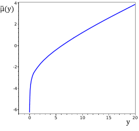
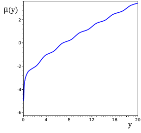
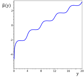
a) b)                                  c) d)

Figure 1: (Colour online) Plot of $\bar{\mu}(y)$ defined in (2.42) for $a=1.2$, $\upsilon=12$ and various values of the attraction parameter: $p=2$ (curve a), $p=3$ (curve b), $p=4$ (curve c), $p=6$ (curve d).

$$a=1.2,\qquad\upsilon=12,$$ (3.1)

and $p=2,3,4,6$ — curves (a), (b), (c) and (d), respectively. In the first two cases, $\bar{\mu}$ is an increasing function, which corresponds to the situation described in theorem 2.1. That is, the values of $p=2$ and $3$ are below the critical value $p_{\text{c}}=p_{\text{c}}(a)$. For $a$ and $\upsilon$ as in (3.1), our calculations yield

$$p_{\text{c}}=3.928235(8).$$

For $p=p_{\text{c}}$, the function $y\mapsto E(y,p_{\text{c}},\mu)$ still has a unique global maximum, which gets degenerate, i.e., $E_{2}(\bar{y},p_{\text{c}},\mu)=0$, cf. (2.20). The value of $\bar{y}=\bar{y}_{\text{c}}$ at which this occurs gives the value of the critical density $\bar{n}_{\text{c}}=\bar{y}_{\text{c}}/p_{\text{c}}$, see (2.28). For various values of the parameter $a$, see (2.4), the values of $p_{\text{c}}(a)$, $\bar{y}_{\text{c}}(a)$ and $\bar{n}_{\text{c}}(a)$ are given in the following table 1.

Table 1: Values of $p(a)$, $\bar{y}(a)$, $\bar{n}(a)$ in the critical point for $v=12$.

$a$	1.0001	1.2	1.5	2	10
$p_{\text{c}}(a)$	3.8255	3.9282	3.9796	3.9973	4.0000
$\bar{y}_{\text{c}}(a)$	2.0485	2.0187	2.0052	2.0007	2.0000
$\bar{n}_{\text{c}}(a)$	0.5355	0.5139	0.5038	0.5005	0.5000

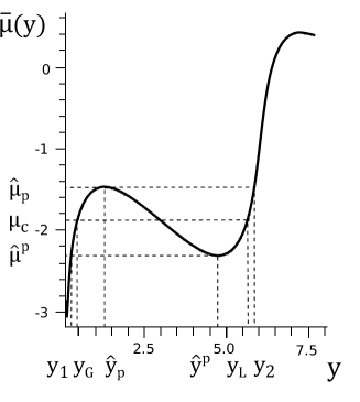
Figure 2: Plot of $\bar{\mu}(y)$ for $a=1.2$ and $p=6$ more in detail.

The values of $p=4$ and $6$ are above the critical point $p_{\text{c}}$, which can be clearly seen from the curves (c) and (d) of figure 1. In this case, one deals with the situation described by theorem 2.2. figure 2 presents more in detail the curve plotted in figure 1 (d), i.e., corresponding to $p=6$ and $a=1.2$. It provides a good illustration to the proof of theorem 2.2. Here, we have $\bar{\mu}(y_{2})=\bar{\mu}(y_{p})$.

Let us now turn to the maximum points of $E(y,p,\mu)$. For $a$ as in (3.1) and $p=6$, figure 3 presents the dependence of $E$ on $y$ for $\mu_{1}=-2.3080$ (curve a), and $\mu_{2}=-1.4700$ (curve b). This provides an illustration to (2.52). The curve plotted in figure 5 corresponds to the critical value of $\mu$ defined by the condition $D(\mu)=0$. That is, $(p,\mu_{\text{c}})$ with $p=6$ and $\mu_{\text{c}}=-1.890291$ is the phase coexistence point whose existence was proved in theorem 2.2. Figure 5 presents the dependence of $E(\bar{y}_{1}(\mu),p,\mu)$ (line 1, red) and $E(\bar{y}_{2}(\mu),p,\mu)$ (line 2, blue) on $\mu\in M_{p}$, $p=6$, cf. (2.51). Their intersection occurs at $\mu=\mu_{\text{c}}=-1.890291$.

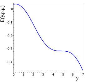
a) b)

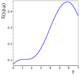
Figure 3: (Colour online) Plot of the function $E(y,p,\mu)$ for $p=6$, $a=1.2$ and $\mu_{1}=-2.3080$ (curve a), $\mu_{2}=-1.4700$ (curve b).

Figure 4: (Colour online) The same as in figure 3 for $\mu=\mu_{\text{c}}=-1.890291$.

Figure 5: (Colour online) Plot of the pressure as a function of temperature in the extremum points of the compressibility. Plot of the functions $M_{p}\ni\mu\mapsto E(y_{i}(\mu),p,\mu)$, $i=1,2$, see (2.51), and $p=6$, $a=1.2$.

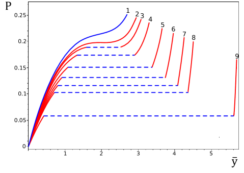
Figure 6: (Colour online) Plot of the dependence of the pressure on $\bar{y}=p\bar{n}$ (isotherms) see (2.27) and (2.28). Curve 1 corresponds to $p=3.8<p_{\text{c}}$. The curves 2–9 correspond to $p\geqslant p_{\text{c}}$: $p=p_{\text{c}}$ (curve 2), $p=4$ (curve 3), $p=4.135$ (curve 4), $p=4.3647$ (curve 5), $p=4.5824$ (curve 6), $p=4.8$ (curve 7), $p=5$ (curve 8), $p=6$ (curve 9).

The curves plotted in figure 6 present the isotherms — the dependence of the pressure on $\bar{y}$, which is equivalent to the dependence on the density $\bar{n}$, see (2.26), calculated from (2.28) for a number of fixed values of $p$.

4 Concluding remarks

In this work, we proved the existence of multiple thermodynamic phases at the same values of the extensive model parameters — temperature and chemical potential. In contrast to the approach of [1], we deal directly with thermodynamic phases in the grand canonical setting. To the best of our knowledge, this is the first result of this kind.

Ukrainian 0

Ôàçîâèé ïåðåõiä ó ñèñòåìi iç ïàðíîþ âçàєìîäiєþ Êþði-Âåéñà

[]Þ.Â. Êîçèöüêèé${}^{\textsf{\footnotesize{\mbox{?}}}}$, Ì.Ï. Êîçëîâñüêèé${}^{\textsf{\footnotesize{\mbox{?}}}}$, Î.À. Äîáóø${}^{\textsf{\footnotesize{\mbox{?}}}}$

             
${}^{\textsf{\footnotesize 1}}$ Iíñòèòóò ìàòåìàòèêè, Óíiâåðñèòåò Ìàði¿ Êþði-Ñêëîäîâñüêî¿,
ïë. Ìàði¿ Êþði-Ñêëîäîâñüêî¿, 1, 20-031 Ëþáëií, Ïîëüùa ${}^{\textsf{\footnotesize 2}}$ Iíñòèòóò ôiçèêè êîíäåíñîâàíèõ ñèñòåì ÍÀÍ Óêðà¿íè, âóë. Ñâєíöiöüêîãî, 1, 79011 Ëüâiâ, Óêðà¿íà

References

- [1] Lebowitz J.L., Penrose O., J. Math. Phys., 1966, 7, 98, doi:10.1063/1.1704821.
- [2] Lebowitz J.L., Mazel A.Z., Presutti E., J. Stat. Phys., 1999, 94, 955, doi:10.1023/A:1004591218510.
- [3] Presutti E., Physica A, 1999, 263, 141, doi:10.1016/S0378-4371(98)00526-3.
- [4] Pulvirenti E., Phase Transitions and Coarce Graining for a System of Particles in the Continuum, Ph.D. Thesis, Roma Tre, 2013, URL http://pub.math.leidenuniv.nl/~pulvirentie/tesi.pdf.
- [5] Pulvirenti E., Tsagkarogiannis D., In: From Particle Systems to Partial Differential Equations III, Springer Proc. in Math. Statistics, Vol. 162, Gonçalves P., Soares A.J. (Eds.), Springer International Publishing Switzerland, 2016, 263–283.
- [6] Ellis R.S., Newman C.M., J. Stat. Phys., 1978, 19, 149, doi:10.1007/BF01012508.
- [7] Külske Ch., Opoku A., J. Math. Phys., 2008, 49, 125215, doi:10.1063/1.3021285.
- [8] Kepa D., Kozitsky Yu., Condens. Matter Phys., 2008, 11, 313, doi:10.5488/CMP.11.2.313.
- [9] Albeverio S., Kondratiev Yu., Röckner M., J. Funct. Anal., 1998, 154, 444, doi:10.1006/jfan.1997.3183.
- [10] Ruelle D., Commun. Math. Phys., 1970, 18, 127, doi:10.1007/BF01646091.
- [11] Fedoryuk M.V., In: Analysis I: Integral Representations and Asymptotic Methods, Encyclopaedia of Mathematical Sciences, Vol. 13, Evgrafov M.A., Gamkrelidze R.V. (Eds.), Springer-Verlag, Berlin, Heidelberg, 1989, 83–191.
- [12] Fritsche K., Grauert H., From Holomorphic Funtions to Complex Manifold, Springer-Verlag, New York, 2002.
Ukrainian \adddialect\l@ukrainian0 \l@ukrainian