Phenomenological Implications of Very Special Relativity

Abstract

We discuss several phenomenological implications of Very Special Relativity (VSR). It is assumed that there is a small violation of Lorentz invariance and the true symmetry group of nature is a subgroup called SIM(2). This symmetry group postulates the existence of a fundamental or preferred direction in space-time. We study its implications by using an effective action which violates Lorentz invariance but respects VSR. We find that the problem of finding the masses of fundamental fermions is in general intractable in the presence of VSR term. The problem can be solved only in special cases which we pursue in this paper. We next determine the signal of VSR in torsion pendulum experiment as well as clock comparison experiment. We find that VSR predicts a signal which is different from other Lorentz violating theories and hence a dedicated data analysis is needed in order to impose reliable limits. Assuming that signal is absent in data we determine the limits that can be imposed on the VSR parameters. We also study the implications of VSR in particle decay experiments taking the charged pion and kaon decay as an example. The effective interaction between the charged pion and the final state leptons is related to the fundamental VSR mass terms through a loop calculation. We also predict a shift in the angular dependence of the decay products due to VSR. In particular we find that these no longer display azimuthal symmetry with respect to the momentum of the pion. Furthermore the azimuthal and polar angle distributions show time dependence with a period of a sidereal day. This time dependence provides us with a novel method to test VSR in future experiments.

I Introduction

Lorentz invariance is experimentally verified to a very high degree of accuracy. Nevertheless, it is interesting to consider models which postulate a small violation of this symmetry. In particular, many quantum gravity models predict breaking of Lorentz invariance at Planck scale energy ($M_{Pl}\approx 10^{19}$ GeV) [1]. It is rather interesting that the observational data already rules out most of these models, except those based on supersymmetry [2, 3, 4, 5]. In such models, violation of Lorentz invariance is suppressed by the factor $\frac{M_{SUSY}^{2}}{M_{Pl}^{2}}$ [4]. In these models the effects of Lorentz violation (LV) grow with energy and are significant only at very high energies.

An alternative framework to implement violation of Lorentz invariance is provided by Very Special Relativity (VSR) [6]. In this framework one postulates that only a subgroup, such as, T(2), E(2), HOM(2) and SIM(2), of the full Lorentz group remains preserved [6]. The generators of HOM(2), for example, are $T_{1}=K_{x}+J_{y}$, $T_{2}=K_{y}-J_{x}$ and $K_{z}$ where $\mathbb{J}$ and $\mathbb{K}$ represent rotation and boost respectively, while those of SIM(2) are $T_{1}$, $T_{2}$, $J_{z}$ and $K_{z}$. A theory which is invariant only under one of these subgroups but not the full Lorentz group, necessarily breaks the discrete symmetries P, T, CP (or CT). However the dispersion relations of particles remain unchanged. Hence several consequence of SR, such as frame invariance of the speed of light, time dilation and velocity addition remain preserved [6, 7]. This also implies that some of the standard high energy tests of LV are not applicable in this case.

It is useful to define a null vector

$$n^{\mu}=(1,0,0,1)\,,$$ (1)

which is invariant under E(2) and T(2) transformations but not under HOM(2) and SIM(2). In this paper we shall primarily be interested in small violations of Lorentz invariance which preserve SIM(2). We shall implement this by using effective Lagrangian approach and construct interaction terms in terms of $n^{\mu}$ which respect SIM(2) but violate Lorentz invariance. The vector $n^{\mu}$ is given by Eq. 1 only in a particular reference frame. In general, the form of $n^{\mu}$ would change under Lorentz transformations and rotations. However it is always possible to make a HOM(2) (and SIM(2)) transformation into the rest frame of a particle [6]. Under these transformations $n^{\mu}$ changes at most by an overall factor which cancels out in the calculation of decay rates. Hence we can choose a frame at rest with respect to the particle or to the laboratory in which $n^{\mu}$ takes the form given in Eq. 1. However the orientation of the particle momentum relative to the z-axis in this frame has to be taken into account while making experimental predictions, as discussed below.

There has been considerable theoretical effort in order to understand the phenomenological implications of VSR [8, 9, 10, 11, 12, 13, 14, 15, 16, 17, 18, 19, 20]. In this paper we illustrate some phenomenological implications of VSR [6] using an effective action approach. We assume that Lorentz violating, VSR effects are small and can be treated perturbatively. We add an effective, gauge invariant VSR invariant mass terms for leptons and quarks to the Standard Model (SM) action. Such a mass term is interesting since it can potentially explain the neutrino masses and mixings without requiring a right handed neutrino. However a detailed analysis of the resulting model is so far lacking in the literature. As we argue in section II, the model in the general case becomes rather intractable and leads to a mathematical structure incompatible with quantum mechanics. Hence we are unable to make reliable predictions in the general case and impose some constraints on the parameter space in order make the problem solvable. We next consider limits that can be imposed on the restricted set of VSR parameters using torsion pendulum [21] and clock comparison experiments [22]. These can impose limits on the VSR contributions to the electron and nucleon masses respectively. The latter can be used to constrain the VSR up and down quark masses. We determine the time dependence of the signal that VSR produces in such experiments due to rotation of the Earth. We find that the signal is different from what is expected in a generic LV theory and requires a dedicated data analysis in order to impose proper limits. We determine the level at which the electron and nucleon masses can be constrained in such experiments.

We also study the implications of VSR for elementary particle decay experiments taking the charged pion and kaon decays as an example. Using the uncertainty in the observed decay rates we impose a limit on the VSR contribution to the up, down and strange quark masses. We also show that VSR leads to anisotropic distribution of decay products in the pion (or kaon) rest frame. Furthermore it leads to azimuthal angle dependence in the laboratory frame. The differential cross section also picks up time dependence due to rotation of the Earth. Similar effects are likely arise in a wide range of decay and scattering processes within VSR. Such effects have so far not been studied within the framework of VSR although some studies have been performed in other Lorentz violating theories [23]. As we have already mentioned, in the latter case the effect is likely to be seen only at very high energies whereas the effects associated with VSR may be observable at low energies. Charged pion decay has been studied to constrain LV in the weak sector [24, 25]. However none of these studies have investigated this decay process within the framework of VSR.

II VSR invariant effective Lagrangian

We work within the framework of a generalized SM in which the Lorentz violating terms which respect VSR are introduced using the effective action approach. The corresponding Lagrangian density can be written as

$${\cal L}={\cal L}_{g}+{\cal L}_{Y}$$ (2)

where we have split the terms into the gauge and the Yukawa sector. The gauge terms for the case of leptons can be written as

$${\cal L}_{g} = i\left(\begin{array}[]{cc}\bar{\nu}_{i}&\bar{e}_{i}\end{array}\right)_{L}\left(\not{\partial}+i{g^{\prime}\over 2}\not{A}-i{g\over 2}\tau\cdot\not{W}\right)\left(\begin{array}[]{c}\nu_{i}\\ e_{i}\end{array}\right)_{L}$$ (6)

$$+ i\bar{e}_{iR}\left(\not{\partial}+ig^{\prime}\not{A}\right)e_{iR}+{\cal L}_{VSR}$$ (7)

where $i$ is the family index and $A_{\mu}$ and $W^{a}_{\mu}$ represent the U(1) and SU(2) gauge fields. The corresponding gauge couplings are denoted by $g_{1}$ and $g_{2}$ respectively. The Lorentz violating, VSR invariant term can be expressed as

$${\cal L}_{VSR} = {i\over 2}\left(\begin{array}[]{cc}\bar{\nu}_{i}&\bar{e}_{i}\end{array}\right)_{L}\left[{\tilde{M}_{L}}^{2}\right]_{ij}{\not{n}\over n\cdot D}\left(\begin{array}[]{c}\nu_{j}\\ e_{j}\end{array}\right)_{L}$$ (11)

$$+ {i\over 2}\bar{e}_{iR}\left[{\tilde{M}_{R}}^{2}\right]_{ij}{\not{n}\over n\cdot D}e_{jR}$$ (12)

where $n^{\mu}$ is the null vector defined in Eq. 1. Here we shall assume that neutrinos do not acquire any mass terms other than those arising out of VSR. The mass matrices $\tilde{M}_{L}^{2}$ and $\tilde{M}_{R}^{2}$ need not be diagonal but have to be Hermitian. We could diagonalize them by a unitary transformation but then the standard mass terms for charged leptons generated through the Yukawa interactions will necessarily be non-diagonal. After expanding the Higgs field ${\cal H}$ around its vacuum expectation value (vev) $v$, the Yukawa terms yield

$${\cal L}_{Y}=-\bar{e}_{iL}M_{{}_{ij}}\,e_{jR}+\left(\begin{array}[]{cc}\bar{\nu}_{i}&\bar{e}_{i}\end{array}\right)_{L}g_{{}_{Yij}}\tilde{\cal H}\,e_{jR}+h.c.$$ (13)

where the mass matrix $M=-g_{Y}v/\sqrt{2}$ , $g_{Y}$ is the Yukawa coupling matrix and $\tilde{\cal H}$ represent the fluctuations of the Higgs field around its vev.

We next diagonalize the mass matrix $M$ by the transformation

$$e_{iL}\rightarrow U_{Lij}e_{jL}\,\,\,\,,\,\,\,e_{iR}\rightarrow U_{Rij}e_{jR}$$ (14)

where $U_{L}$ and $U_{R}$ are unitary matrices. Furthermore we diagonalize the VSR neutrino $\tilde{M}_{L}^{2}$ by the transformation

$$\nu_{iL}\rightarrow V_{Lij}\nu_{jL}$$ (15)

The VSR charged lepton mass terms can now be written as [9, 20]

$${\cal L}_{VSR} = {i\over 2}\bar{\nu}_{iL}M_{\nu ij}^{2}{\not{n}\over n\cdot D}\nu_{jL}+{i\over 2}\bar{e}_{iL}\left[M_{L}^{2}\right]_{ij}{\not{n}\over n\cdot D}e_{jL}$$ (16)

$$+ {i\over 2}\bar{e}_{iR}\left[M_{R}^{2}\right]_{ij}{\not{n}\over n\cdot D}e_{jR}$$

where $M^{2}_{\nu}$ is a diagonal matrix and $M_{L}^{2}=U_{e}^{\dagger}M_{\nu}^{2}U_{e}$ and $M_{R}^{2}=U_{R}^{\dagger}\tilde{M}_{R}^{2}U_{R}$ are non-diagonal charged lepton mass matrices. Here $U_{e}=U^{\dagger}_{L}V$ is the neutrino mixing matrix. The resulting Lagrangian nicely explains the neutrino masses and mixings but considerably complicates the propagation of charged leptons. The charged lepton Dirac equation gets modified to

$$\left[\not{p}-M_{D}-{1\over 2}M_{+}^{2}{\not{n}\over n\cdot p}-{1\over 2}M_{-}^{2}{\not{n}\gamma_{5}\over n\cdot p}\right]\psi=0$$ (17)

where $M_{D}$ is the diagonal Dirac mass matrix,

$$\psi=\left(\begin{array}[]{c}e\\ \mu\\ \tau\end{array}\right)$$

is a 12 component lepton multiplet with $e$, $\mu$ and $\tau$ representing the 4 component Dirac spinors for these leptons and $M_{\pm}^{2}=(M_{L}^{2}\pm M_{R}^{2})/2$.

The matrix $M_{L}^{2}$ is fixed by the neutrino masses and mixings whereas $M_{R}^{2}$ is completely unknown. Hence, excluding some special cancellations, we expect that in general both $M_{\pm}^{2}$ would be non-zero and non-diagonal. This makes Eq. 17 rather complicated and untractable since it leads to mixing both between different spinors as well as between families. Furthermore it does not even lead to a Hamiltonian structure. We see this by going to the non-relativistic limit and setting the three momentum $\vec{p}=0$. In this limit the equation can be written as

$$H\psi=E\psi$$ (18)

where $H$ is the generalized Dirac Hamiltonian

$$H=\gamma^{0}M_{D}+{M_{+}^{2}\over 2E}\Gamma+{M_{-}^{2}\over 2E}\Gamma\gamma^{5}\,,$$ (19)

$\Gamma=1-\gamma^{0}\gamma^{3}$. Let us first consider the simpler case in which the matrices $M_{+}^{2}$ and $M_{-}^{2}$ are diagonal. In this case we can treat each generation of fermions independently. Hence we focus on a single four component spinor and set $M_{D}$, $M_{+}^{2}$ and $M_{-}^{2}$ equal to their corresponding diagonal entries $m_{D}$, $m_{+}^{2}$ and $m_{-}^{2}$ respectively. However due to the presence of $(n\cdot\partial)^{-1}$ in the original equation, the Hamiltonian itself depends on the energy eigenvalue $E$, which in the present case is equal to the mass of the particle. The solution for this case is given in [9]. The eigenvalues are found to be $E(\uparrow)=\sqrt{m_{D}^{2}+m_{+}^{2}-m_{-}^{2}}$ and $E(\downarrow)=\sqrt{m_{D}^{2}+m_{+}^{2}+m_{-}^{2}}$ for the positive energy (electron) spinors with spin up and down respectively. Similar results are obtained for anti-particles which are degenerate with particles. Here we use the non-relativistic limit and focus on the particle states.

The important point is that the energy eigenvalues of the spin up and down states are not degenerate. This means that the Hamiltonian is different for these two states and hence does not really get diagonalized. In other words the eigenvectors for spin up and down are eigenvectors of different Hamiltonians and hence we are unable to construct a unitary operator which will diagonalize the Hamiltonian. This means that the mathematical structure of VSR is not consistent with the standard framework of quantum mechanics. We are not sure how to mathematically solve this problem and do not pursue it further in full generality. However, as discussed below, we find that there are some limiting cases in which the problem is tractable.

The problem is obvious directly from Eq. 19. We work in the Dirac-Pauli representation in which $\gamma^{0}$ is diagonal. Due to presence of $E$ in the last two terms in this equation, diagonalization of $H$ is possible only if (i) the operator $m_{+}^{2}\Gamma+m_{-}^{2}\Gamma\gamma^{5}$ is diagonal or (ii) All eigenvalues of H are degenerate. The first possibility is not realized for any choice of values of $m_{+}^{2}$ and $m_{-}^{2}$ while the second is found to be true if $m_{-}^{2}=0$. We see this directly by the eigenvalues $E(\uparrow)$ and $E(\downarrow)$ given above. Hence in this case the problem mentioned above no longer appears and the eigenvectors will correspond to a unique Hamiltonian. We shall impose this condition for further analysis. In earlier work [9] it has been argued that $m_{-}^{2}$ is very strongly constrained by observations. This may be correct but we have argued that it is really not possible to reliably determine the experimental implications of the theory if $m_{-}^{2}\neq 0$. Hence it is not possible to impose reliable constraints on this parameter.

We next consider the general case in which mass matrix $M_{+}^{2}$ is not diagonal. We continue to set $M_{-}^{2}=0$ based on the arguments presented above. In this case the energy eigenvalues are clearly not degenerate since different charged leptons have different masses. Hence the system can be solved only if the matrix $M_{+}^{2}$ is diagonal which is just the limit discussed above. However if we assume that neutrino masses are generated entirely by the VSR mass terms, then $M_{+}^{2}=U_{e}^{\dagger}M_{\nu}^{2}U_{e}$ is necessarily non-diagonal. Based on our arguments above, this case cannot be treated reliably and we do not pursue it further. Only by assuming a diagonal form for the matrix $M_{+}^{2}$ can we impose reliable limits on the VSR parameters. This of course significantly reduces the interest in further pursuing this formalism. Nevertheless we feel that it is an interesting theory of Lorentz violation and continue to investigate its phenomenological consequences. Furthermore it is possible that mathematical framework may be developed in future which may give a reliable solution to the problem in the general case.

The situation with VSR quark masses is similar. We have an effective Lorentz violating, VSR Lagrangian similar to Eq. 12 with left and right handed terms both for up and down type quark multiplets. This can be expressed as

$${\cal L}^{q}_{VSR} = {i\over 2}\left(\begin{array}[]{cc}\bar{u}_{i}&\bar{d}_{i}\end{array}\right)_{L}\left[{\tilde{M}_{Lq}}^{2}\right]_{ij}{\not{n}\over n\cdot D}\left(\begin{array}[]{c}u_{j}\\ d_{j}\end{array}\right)_{L}$$

$$+ {i\over 2}\bar{u}_{iR}\left[{\tilde{M}_{Ru}}^{2}\right]_{ij}{\not{n}\over n\cdot D}u_{jR}$$

$$+ {i\over 2}\bar{d}_{iR}\left[{\tilde{M}_{Rd}}^{2}\right]_{ij}{\not{n}\over n\cdot D}d_{jR}$$ (24)

In principle, these mass matrices can be non-diagonal [9, 20]. Here we work in the basis in which the Dirac mass matrices are diagonal. For reasons discussed above for the case of leptons, the Hamiltonian in this case also admits energy eigenvalues and eigenvectors only in the case in which the VSR mass matrices are diagonal. Hence we impose this restriction for further analysis. Furthermore we set $M_{-}^{2}=(M_{L}^{2}-M_{R}^{2})/2=0$ for reasons given earlier.

III Limits based on torsion pendulum

We next consider the limits that can be imposed on the VSR masses based on the spin pendulum experiment. Here we set $M_{-}^{2}=0$ and assume that $M_{+}^{2}$ is diagonal both for quarks and leptons. The basic framework has been developed in [9] which can be applied to electrons. In the non-relativisitic limit, the relevant term in the effective Hamiltonian in the $n\cdot A=0$ gauge is given by [9]

$$H_{VSR}=-\epsilon\mu_{B}(\hat{n}\cdot\vec{\sigma})(\hat{n}\cdot\vec{B})$$ (25)

where $\vec{B}$ is the background magnetic field, $\hat{n}$ is the spatial component of the vector $n^{\mu}$, $\mu_{B}=e\hbar/(2m_{e}c)$, $\epsilon=m_{+}^{2}/m_{e}^{2}$, $m_{e}$ is the electron mass and $m_{+}^{2}$ is the VSR contribution to the electron mass. By using the results of Penning trap experiment with a single trapped electron [26] it was found that $\epsilon\lesssim 10^{-11}$ [9]. It may be possible to impose a more stringent limit by using the experimental results on torsion pendulum [21]. However it is not possible to directly use the limits given in [21]. This is because those limits have been obtained by assuming that the effect has a time period of 1 sidereal day. However Eq. 25 shows that the effect is more complicated. In particular, as discussed below, it shows two oscillations in 1 sidereal day.

Let us denote the equatorial coordinate system by $xyz$ and the laboratory system by $abc$. We choose coordinates such that z-axis is parallel to the rotation axis of the Earth and x-axis points towards the vernal equinox. Let the equatorial coordinates of the vector $\hat{n}$ be $(\theta_{e},\phi_{e})$ where $\phi_{e}$ is the Right Ascension and $\theta_{e}$ is the polar angle (Declination = $\pi/2-\theta_{e}$). Let the unit vectors along the axis $a,b,c$ of the local frame be $\hat{i},\hat{j}$ and $\hat{k}$ respectively. We take the vector $\hat{k}$ to point vertically upwards and vectors $\hat{i}$ and $\hat{j}$ tangential to the surface pointing towards north and west respectively. The two coordinate systems are related by the formula

$$\hat{x} = \cos(\theta+\alpha)\hat{j}-\sin(\theta+\alpha)(\cos\lambda\hat{k}-\sin\lambda\hat{i})$$

$$\hat{y} = \sin(\theta+\alpha)\hat{j}+\cos(\theta+\alpha)(\cos\lambda\hat{k}-\sin\lambda\hat{i})$$

$$\hat{z} = \cos\lambda\hat{i}+\sin\lambda\hat{k}$$ (26)

where $\theta=\Omega t$, $\alpha$ is the Right Ascension of $\hat{j}$ at $t=0$, $\lambda$ is the latitude of the observer, $\Omega=2\pi/T_{0}$ and $T_{0}$ is one sidereal day.

The spin of the torsion pendulum used in [21] is aligned horizontally. Hence we set the magnetic moment $\vec{m}$ of the pendulum equal to $m_{1}\hat{i}+m_{2}\hat{j}$. The magnetic field $\vec{B}=B_{1}\hat{i}+B_{2}\hat{j}$ also points in the same direction as $\vec{m}$ and hence $B_{1}/B_{2}=m_{1}/m_{2}$. Using this we can determine the torque experienced by a single electron due to VSR effects. The torque about the local normal is found to be

$$\tau_{b} = \epsilon\hat{n}\cdot\vec{B}\bigg{\{}m_{1}\sin\theta_{e}\cos(\theta+\alpha-\phi_{e})$$ (27)

$$- m_{2}\sin\theta_{e}\sin\lambda\sin(\theta+\alpha-\phi_{e})$$

$$- m_{2}\cos\theta_{e}\cos\lambda\bigg{\}}$$

where

$$\hat{n}\cdot\vec{B} = B_{1}\bigg{[}\sin\lambda\sin\theta_{e}\sin(\theta+\alpha-\phi_{e})+\cos\lambda$$ (28)

$$\times \cos\theta_{e}\bigg{]}+B_{2}\sin\theta_{e}\cos(\theta+\alpha-\phi_{e})$$

The experimentalists [21] split data into torques generated by the north and west components of the effective field $\vec{\beta}$ which couples to $\vec{m}$, such that the energy $E\propto-\vec{\beta}\cdot\vec{m}$. In our case this corresponds to $n_{1}$ and $n_{2}$ respectively times an overall factor $\epsilon\hat{n}\cdot\vec{B}$. The corresponding torques generated by these components are given by the terms proportional to $m_{2}$ and $m_{1}$ respectively in Eq. 27. The overall expression is different from what is assumed in the analysis performed in [21]. Hence we suggest that the data should be reanalyzed in order to impose constraints on VSR parameters. In Fig. 1 we show a representative graph of our results setting $m_{1}/m_{2}=1$. We clearly see that the signal shows two oscillations within one sidereal day. Hence a dedicated analysis is needed in order to obtain reliable limits on VSR parameters. Assuming that no signal is found, the torsion pendulum experiment [21] will impose limit on $\epsilon$ such that $\epsilon\lesssim 10^{-20}\ {\rm eV}/(\mu_{B}B)$ which will imply $\epsilon\lesssim 10^{-15}$.

Figure 1: The predicted signal for the torques generated in the torsion pendulum [21] in arbitrary units for a randomly chosen set of parameters $\theta_{e}=0.6\pi$ and $\alpha-\phi_{e}=\pi/2$. The solid and dotted curves refer to $\beta_{W}$ and $\beta_{N}$ using the notation of [21]. The latitude $\lambda$ has been set equal to that of the observer location. We have also set $m_{1}/m_{2}=B_{1}/B_{2}=1$.

III.1 Limits on VSR nucleon mass using clock comparison experiments

We next consider bounds that can be imposed on VSR contribution to nucleon mass using clock comparison experiments [27, 28, 29, 30] with polarized nucleons [31, 32, 22]. Let $\tilde{m}_{n}^{2}$ be the VSR contributions to the nucleon mass. We assume isospin symmetry and set the proton and neutron mass equal to one another. Furthermore we treat nucleon as a Dirac particle with an effective magnetic moment described by the g-factor of proton or neutron. We also ignore nuclear effects which have to be included for a detailed fit. As argued earlier we only allow contributions which are proportional to $\not{n}$ and set the contribution proportional to $\not{n}\gamma_{5}$ to zero. The VSR nucleon mass may be related to the up and down quark VSR masses, denoted by $\tilde{m}_{q}^{2}$, of up and down quarks by a form factor $G_{n}$. Hence we expect $\tilde{m}_{n}^{2}=G_{n}\tilde{m}_{q}^{2}$.

We consider an experiment with polarized neutrons or protons, with their spins vertically upwards. The VSR effect will lead to a shift in the precession frequency of the nucleons. The effect has already been considered in [9] for the case of electrons. Essentially we can incorporate the effect by defining an effective magnetic field $\vec{B}^{\prime}=\vec{B}+(2/g)\epsilon_{n}\hat{n}(\hat{n}\cdot\vec{B})$, where $g$ is the g-factor of the particle, proton or neutron, $\epsilon_{n}=\tilde{m}_{n}^{2}/m_{n}^{2}$ and $m_{n}$ is the nucleon mass. The magnetic field in this case points along $\hat{k}$ and hence the frequency gets shifted by the factor $(1+\xi)$ where $\xi=(2/g)\epsilon_{n}(\hat{n}\cdot\hat{k})^{2}$. We obtain

$$\hat{n}\cdot\hat{k}=\cos\theta_{e}\sin\lambda-\sin\theta_{e}\cos\lambda\sin(\theta+\alpha-\phi_{e})$$ (29)

We plot $\xi$ for arbitrarily chosen parameters in Fig. 2. We again clearly see that the signal is not just a simple sinusoidal variation with a period of a sidereal day. Instead we see two oscillations with varying amplitude within one sidereal day. Hence a dedicated search is needed in order to constrain the VSR parameters. Assuming that the signal is absent in the data, we can obtain the bound $\epsilon_{n}\mu_{N}B\lesssim 10^{-31}$ GeV using the experimental data from [22], where $\mu_{N}=e\hbar/(2m_{n}c)$. This will lead to the limit $\epsilon_{n}\lesssim 10^{-11}$ where we have used $B\approx 1.5$ G. This leads to $\tilde{m}_{n}^{2}\lesssim 10^{7}$ eV².

Figure 2: The predicted signal for $\xi$, the shift in the precession frequency of nucleon (in arbitrary units) due to VSR effects. Here we have chosen the same set of parameters $(\theta_{e},\alpha-\phi_{e},\lambda)$ as in Fig. 1.

IV Pion Decay

We next consider implications of VSR for elementary particle physics experiments. Here we are primarily interested in effects which arise due to rotation of Earth. We shall illustrate the effect by considering the decay of pion as an example. Similar effects are expected in other processes. The decay amplitude within the SM can be computed by introducing the following effective interaction term:

$${\cal L}_{\pi,SM}=V_{ud}\frac{G_{f}}{\sqrt{2}}{f}_{\pi}\partial_{\mu}\pi^{-}\bar{\psi_{l}}\gamma^{\mu}(1-\gamma^{5})\psi_{\nu}+h.c.\,,$$ (30)

where $\pi^{-}$, $\psi_{l}$ and $\psi_{\nu}$ represent the charged pion, charged lepton and the neutrino fields respectively. Here $f_{\pi}=132$ MeV is the pion decay constant, $V_{ud}=\cos\theta_{c}$ is the CKM matrix element and $\theta_{c}$ the Cabibbo angle. This leads to the standard formula for the weak differential decay rate of pions.

The basic Lorentz violating, VSR invariant terms for quarks are given in Eq. 24. Due to the presence of gauge covariant derivative, the VSR terms also lead to Lorentz violating VSR invariant interaction terms of fermions with electroweak gauge bosons as well as gluons for the case of quarks [19, 20]. As argued earlier we require the resulting VSR quark mass matrices to be diagonal and furthermore set $M_{-}^{2}=0$. As we shall show below VSR terms in Eq. 24 lead to an effective Lagrangian density for the coupling of pions with leptons which can be written as

$${\cal L}_{\pi} = {\cal L}_{\pi,SM}+\tilde{g}\left(\frac{n_{\mu}}{n.\partial}\pi^{-}\right)\bar{\psi}_{l}\gamma^{\mu}(1-\gamma^{5})\psi_{\nu}$$ (31)

$$+ h.c.,$$

where $n^{\mu}$ is given by Eq. 1. The first term gives the standard decay amplitude for pion. The second term respects SIM(2) but violates Lorentz invariance due to the presence of preferred axis $n^{\mu}$ [8].

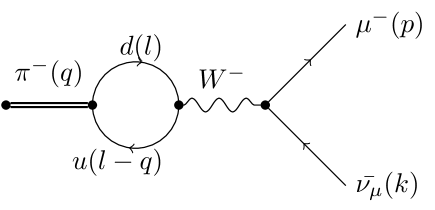
Figure 3: The Lorentz violating matrix term arises from quark VSR modified propagator and lepton-W boson vertex correction in the VSR modified SM Lagrangian.

We next provide a justification for the Lorentz violating effective operator in Eq. 31 using linear sigma model for strong interactions and VSR modified SM Lagrangian which has mass terms of the form given in Eqs. 12 and 24 for all fermions. Alternatively we may use a model pion wave function [33] for this calculation. Here we are primarily interested in demonstrating that this loop leads to a non-zero answer and hence our use of linear sigma model is justified. However a quantitatively reliable estimate of this loop is not possible due to the standard uncertainties in handling strong interactions. We consider linear sigma model at the quark level which contains the fermion field multiplet $\begin{pmatrix}u\\ d\end{pmatrix}$ and the meson multiplet $\sigma+i\tau\cdot\pi\gamma^{5}$, where $\sigma$ is a scalar field. The model leads to an interaction between pseudoscalar pion field and the quark doublet of the form

$${\cal L}_{\sigma}=g^{\prime}\begin{pmatrix}\bar{u}_{i}&\bar{d}_{i}\end{pmatrix}(\sigma+i\tau.\pi\gamma^{5})\begin{pmatrix}u_{i}\\ d_{i}\end{pmatrix},$$ (32)

where $g^{\prime}$ is the coupling and $i$ is the color index. The pion decay into a lepton pair can be represented by the diagram shown in Fig. 3. The coupling of pion with the up and down quarks is given by the linear sigma model. The Lorentz violating VSR invariant contributions arise due to the modification to the up and down quark propagators and the interaction vertex of $W$ boson with quarks. The VSR modified fermion propagator can be written as,

$$\frac{\not{l}+m-\frac{\tilde{m}^{2}}{2}\frac{\not{n}}{n.l}}{l^{2}-m^{2}-\tilde{m}^{2}+i\epsilon}\,.$$

where $m$ is the standard mass arising due to a Lorentz invariant term and $\tilde{m}$ is the VSR mass. We shall assume that for all fermions, except the neutrinos, $\tilde{m}<<m$. The interaction terms arise due to the gauge covariant derivative in Eq. 24. We expand $1/n\cdot D$ in powers of the gauge coupling and keep only the leading order term in this coupling. The modified lepton-W boson vertex is found to be

$$\frac{g}{\sqrt{2}}\left[\gamma^{\mu}+\tilde{m}^{2}\frac{\not{n}n^{\mu}}{2(n\cdot l)(n\cdot(l-q))}\right](1-\gamma^{5})\,.$$

The Feynman amplitude shown in Fig. 3 generates an effective vertex between the pion and the leptons. We can obtain the effective coupling by evaluating the Feynman amplitude for the quark loop in Fig. 3, which can be expressed as,

$$g^{\prime}\frac{g}{\sqrt{2}}\int\frac{d^{4}l}{(2\pi)^{4}}tr\Big{[}\frac{\not{l}+m_{d}-\frac{\tilde{m}_{q}^{2}}{2}\frac{\not{n}}{n.l}}{l^{2}-(m_{d}^{2}+\tilde{m}_{q}^{2})+i\epsilon}\left(\gamma^{\mu}+\tilde{m}_{q}^{2}\frac{\not{n}n^{\mu}}{2n.ln.(l-q)}\right)(1-\gamma^{5})\frac{(\not{l}-\not{q})+m_{u}-\frac{\tilde{m}_{q}^{2}}{2}\frac{\not{n}}{n.(l-q)}}{(l-q)^{2}-(m_{u}^{2}+\tilde{m}_{q}^{2})+i\epsilon}\gamma^{5}\Big{]}$$ (33)

where $\tilde{m}_{q}=\tilde{m}_{u}=\tilde{m}_{d}$. We note that for the left handed up and down quarks the VSR masses have to be equal by gauge invariance. In evaluating this loop we consider terms only up to order $\tilde{m}_{q}^{2}$ because of our assumption $\tilde{m}_{q}<<m_{u},m_{d}$. It is also important to notice that the VSR invariant, Lorentz violating terms are nonlocal.

The Lorentz violating or nonlocal part of the above expression becomes

$$g^{\prime}\frac{g}{\sqrt{2}}\tilde{m}_{q}^{2}n^{\mu}\int\frac{d^{4}l}{(2\pi)^{4}}\Big{(}\frac{4m_{d}\,n\cdot q}{n.l\hskip 3.0ptn.(l-q)(l^{2}-m_{d}^{2}+i\epsilon)((l-q)^{2}-m_{u}^{2}+i\epsilon)}$$

$$+\frac{4m_{u}}{n.(l-q)(l^{2}-m_{d}^{2}+i\epsilon)((l-q)^{2}-m_{u}^{2}+i\epsilon)}-\frac{4m_{u}}{n.l(l^{2}-m_{d}^{2}+i\epsilon)((l-q)^{2}-m_{u}^{2}+i\epsilon)}\Big{)}$$ (34)

After integrating over $l$ the result can only depend on the momentum of the pion, i.e. $q$. Hence the integral leads to an overall factor of $1/n\cdot q$. This gives us an effective interaction of the form given in Eq. 31. We next perform this integral in the rest frame of pion.

The presence of nonlocal term in the fermion propagator inside the loop results in infrared (IR) divergences. It is not practical to use Feynman parametrization for evaluating the above integral because of the presence of nonlocal terms, i.e. $\frac{1}{n.l}$ and $\frac{1}{n.(l-q)}$. There doesn’t exist any reliable procedure for handling these infrared divergences in the literature. We handle this divegence by adding a small imaginary part to the mass of the particle. This amounts to adding a small imaginary part to the energy of an on-shell particle. Hence we replace

$${1\over n\cdot l}\rightarrow{1\over n\cdot(l+i\epsilon^{\prime})}$$ (35)

where $\epsilon^{\prime}$ is a four vector with time component ($\epsilon^{\prime}_{0}>0$) non-zero and space components zero. This prescription may be justified by considering the action of the operator $1/n\cdot\partial$ on a charged scalar field $\phi$. The Fourier decomposition of this may be expressed as

$$\phi=\int{d^{3}k\over(2\pi)^{3}2\omega_{k}}\left[e^{-ik\cdot x}a(k)+e^{ik\cdot x}b^{\dagger}(k)\right]$$ (36)

Action of the operator $1/n\cdot\partial$ on this field should result in the factor $1/n\cdot k$. In order to explicitly implement this we need a prescription for $1/n\cdot\partial$ which essentially is equivalent to an integral. We follow a prescription which is analogous to the one used in Ref. [17]. For the positive frequency part, we set

$${1\over n\cdot\partial}f^{+}(x)\rightarrow\int_{-\infty}^{x_{+}}dx^{\prime}_{+}f^{+}(x^{\prime})$$ (37)

whereas for the negative frequency we use

$${1\over n\cdot\partial}f^{-}(x)\rightarrow-\int_{x_{+}}^{\infty}dx^{\prime}_{+}f^{-}(x^{\prime})\,.$$ (38)

Here $x_{+}=(t+z)/2$. Let us now apply this operator to the positive frequency part. We obtain

$${1\over n\cdot\partial}\phi^{+}(x)=\int{d^{3}k\over(2\pi)^{3}2\omega_{k}}{1\over-ik_{-}}\left[e^{-ik_{-}x_{+}}-e^{ik_{-}\infty}\right]e^{-ik\cdot x+ik_{-}x_{+}}a(k)$$ (39)

where $k_{-}=k^{0}-k^{3}=n\cdot k$. This clearly gives us the expected result as long as the second term in the bracket goes to zero. This is true if $k^{0}$ contains a small imaginary part as prescribed above. Similarly we can check that the negative frequency part leads to the expected result with our prescription.

The loop integral is evaluated by performing the integral over $l^{0}$ analytically and over the spatial components numerically. The numerical calculations are performed by using a small non-zero value of the infrared regulator $\epsilon^{\prime}_{0}$ of the order of a few MeV. We have verified that the final result is insensitive to the precise choice of this regulator provided it is sufficiently small. For $m_{d}=4.8$ MeV, $m_{u}=2.3$ MeV and $m_{\pi}=139.5$ MeV, we obtain the result $-N_{c}g^{\prime}\frac{g}{\sqrt{2}}\tilde{m}_{q}^{2}n^{\mu}\times 0.092$ where $N_{c}=3$ is the number of colors. Hence the loop gives a non-zero result and generates an effective vertex given in Eq. 31. As already mentioned we can only trust this result qualitatively and not quantitatively due to our inability to reliably handle strong interactions.

IV.1 pion decay in the rest frame

In this section we compute the decay rate of charged pion ($\pi^{-}(q)\rightarrow\mu^{-}(p)+\bar{\nu}_{\mu}(k)$) in its rest frame within the VSR framework. We consider $|\mathfrak{M}|^{2}$ upto leading order in $\tilde{g}$ because the LV parameters are expected to be very small. We obtain

$$|\mathfrak{M}|^{2}=4G_{f}^{2}\mathfrak{f}_{\pi}^{2}V_{ud}^{2}m_{\mu}^{2}(p.k)+\frac{16}{\sqrt{2}}\tilde{g}G_{f}f_{\pi}V_{ud}\left(\frac{(n.p)(q.k)}{n.q}+\frac{(n.k)(p.q)}{n.q}-\frac{(n.q)(p.k)}{n.q}\right)+O(\tilde{g}^{2})$$ (40)

This is valid in general and not just the rest frame.

As explained above, we can always make a SIM(2) transformation to the rest frame of a particle. Our action is invariant under this transformation, although the vector $n^{\mu}$ changes by an overall constant. However the change cancels out in the amplitude. Here we work in a frame ($S$) in which the vector $n^{\mu}$ is given by Eq. 1 up to an overall constant. The LV contribution is assumed to arise entirely from the interaction term in Eq. 31. We point out that the VSR invariant quadratic terms do not change the dispersion relations [8]. Hence the kinematics of the incoming and outgoing particles remain unchanged. The dominant LV contribution to the differential decay rate arises due to SM and LV interference term. This leads to a contribution proportional to $\tilde{g}(1+\cos\theta)$ where $\theta$ is the angle between the muon three momentum and the $z$-axis in the fundamental frame $S$.

We next impose a direct limit on $\tilde{g}$ by assuming that the standard observed value of the pion decay rate arises entirely from the Standard Model and demanding that the LV terms give a contribution less than the error in the observed value. A more detailed limit by studying the angular distributions of the final state can also be imposed. In the next section we shall work out the theoretical formalism required for such a study. However a detailed implementation can only be performed by an experimental group and is beyond the scope of current paper. We point out that here we are only interested in direct experimental limit that can be imposed on this LV parameter. Through loop corrections this parameter may lead to LV contribution to electron propagator. However such contributions only add to the LV parameters in the leptonic sector of the action which can be adjusted to agree with experimental limits. This might require some fine tuning of parameters.

The life time ($\tau$) of the charged pion is $(2.6033\pm 0.0005)\times 10^{-8}$s [34]. The uncertainty in the theoretical calculation of the pion decay rate is approximately 0.2%. Hence we see that the theoretical uncertainty dominates. This leads to the limit, $\tilde{g}<g_{0}$ where $g_{0}=2.2\times 10^{-11}$ GeV. We can relate this to the VSR up and down quark mass parameter $\tilde{m}_{q}$ through the loop shown in Fig. 3 and impose a limit on this parameter. We fix the linear sigma model parameter $g^{\prime}$ by using the standard relation $M_{q}=g^{\prime}f_{\pi}$, where $M_{q}\approx 330$ MeV [35] is the constituent quark mass of up and down quarks. We obtain $\tilde{m}_{u,d}\lesssim 3$ MeV. We notice that the limit is not very stringent and is much weaker than that obtained by using clock comparison experiments assuming that the nucleon form factor $G_{n}$ is of order unity.

The relative change of differential decay rate can be expressed as

$$\Delta = \frac{\frac{d\Gamma}{d\Omega}|_{\tilde{g}\not{=}0}-\frac{d\Gamma}{d\Omega}|_{\tilde{g}=0}}{\frac{d\Gamma}{d\Omega}|_{\tilde{g}=0}}$$ (41)

$$= {2\sqrt{2}\tilde{g}\over f_{\pi}m_{\pi}^{2}G_{f}|V_{ud}|}\left[1+\cos\theta\right]\,.$$

Hence we find that even in the rest frame of pion, the muon distribution is not isotropic and depends on the polar angle $\theta$ due to the LV contributions. The dependence provides a qualitatively new test of LV theories which respect VSR.

IV.2 Kaon Decay

The above formalism can be directly applied to the charged kaon decay $K^{-}(q)\rightarrow\mu^{-}(p)+\bar{\nu}_{\mu}(k)$. We compute the loop integral corresponding to the quark loop shown in Fig. 3 by replacing the down quark with a strange quark. The Lorentz violating part of the loop integral in this case is found to be $N_{c}g^{\prime}\frac{g}{\sqrt{2}}\tilde{m}_{q}^{2}\times 2.32$. Furthermore we use $M_{s}=g^{\prime}f_{K}$ where $M_{s}\approx 550$ MeV [35] is the constituent mass of the strange quark. Using the known uncertainty in the kaon decay rate we impose the limit $\tilde{g}<1.0\times 10^{-10}$ GeV. In this case the theoretical and experimental errors are comparable to one another and we add the two in quadratures in order to obtain the limit on $\tilde{g}$. This leads to a limit $\tilde{m}_{s}\lesssim 1.3$ MeV on the VSR contribution to strange quark mass.

IV.3 pion decay in the laboratory frame

In this section, we determine the differential decay rate assuming that pion has non-zero momentum in the laboratory frame. It is useful to define two frame $S$ and $S^{\prime}$, both at rest with respect to the laboratory. In frame $S$, $n^{\mu}$ is given by Eq. 1 up to an irrelevant overall constant. Let us now consider a beam of pions moving along the $z^{\prime}$ direction making an angle $\theta$ with the preferred axis, as shown in Fig. 4. Let $q$, $p$ and $k$ denote the momenta of $\pi^{-}$, $\mu^{-}$ and $\bar{\nu}$ respectively. Here $xyz$ and $x^{\prime}y^{\prime}z^{\prime}$ refer to $S$ and $S^{\prime}$ coordinate systems respectively. We have used rotational symmetry about the $z$-axis in the frame $S$ in order to choose $x$-axis such that $y^{\prime}$ is aligned with the $y$-axis. Hence $z^{\prime}$ and $x^{\prime}$ lie in the $x-z$ plane. The final state muon makes an angle $\theta^{\prime}$ w.r.t. the beam, i.e. the $z^{\prime}$ axis.

Figure 4: Here $z$ denotes the preferred axis and $x,y$ some chosen coordinate axes. The beam direction is taken to be along the $z^{\prime}$-axis which makes an angle $\theta$ relative to $z$-axis. The axis $x^{\prime}$ is chosen to lie in the $x-z$ plane. Hence the $y$ and $y^{\prime}$ axes, pointing into the plane of the paper, coincide with one another. The momentum of the muon, denoted by $\vec{p}$, makes an angle $\theta^{\prime}$ relative to the $z^{\prime}$-axis.

We find that the differential decay rate picks up a small correction to the $\theta^{\prime}$ dependence of the decay rate due to the LV term. Furthermore it induces a $\phi^{\prime}$ dependence of the final state muon distribution, which is absent in the SM. The $\phi^{\prime}$ dependence of the decay rate can be quantified by defining

$$\Delta^{\prime}=\frac{\frac{d\Gamma}{d\phi^{\prime}}-\Gamma_{avg}}{\Gamma_{avg}}$$ (42)

where $\Gamma_{avg}=\frac{1}{2\pi}\int_{0}^{2\pi}\frac{d\Gamma}{d\phi^{\prime}}d\phi^{\prime}$ is the decay rate averaged over $\phi^{\prime}$. In Fig.(5) we plot $\Delta^{\prime}$ as a function of $\phi^{\prime}$ for the choice of parameters, pion energy $E=200$ MeV and $\theta=\pi/4$. We see that the distribution peaks at $\phi^{\prime}=\pi$ and is minimum at $\phi^{\prime}=0$. From Fig. 4 we see our choice of coordinate system is such that the beam axis, i.e. $z^{\prime}$, lies in the $x^{\prime}-z$ plane. Hence $\phi^{\prime}$ is the azimuthal angle in the $x^{\prime},y^{\prime},z^{\prime}$ coordinate system which is chosen such that $z^{\prime}$ lies in the $x^{\prime}-z$ plane

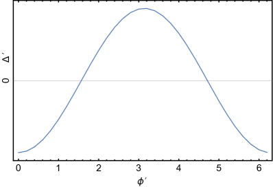
Figure 5: The azimuthal angle $\phi^{\prime}$ dependence of the final state muon distribution. The observable $\Delta^{\prime}$ is defined in Eq. 42. The amplitude of the effect depends on the unknown VSR parameter $\tilde{g}$ or equivalently $\tilde{m}_{u,d}^{2}$ for which we only have an upper limit.

IV.4 Daily Variation

The angle between the preferred axis and the beam direction is expected to change with time due to rotation of Earth. Due to this change the contribution to the differential decay rate arising from the LV term is expected to show periodic variation with a period of 1 sidereal day. Both the observables $\Delta$ and $\Delta^{\prime}$ are expected to show time dependence. In particular we expect that the peak position of $\Delta^{\prime}$ as a function of the azimuthal angle $\phi^{\prime}$ in laboratory frame will show a periodic shift with time.

Let us assume that an observer is located at the latitude $\lambda$. We choose a local laboratory coordinate system at this location, denoted by $x^{\prime\prime}y^{\prime\prime}z^{\prime\prime}$. Here $z^{\prime\prime}$ is along the direction of the beam and $y^{\prime\prime}$ is chosen along the local vertical. It is also convenient to define another local frame $x^{\prime}y^{\prime}z^{\prime}$ such that $z^{\prime}$ is along the beam direction, i.e. same as $z^{\prime\prime}$ and $x^{\prime}$ lies in the $z-z^{\prime}$ plane. We denote the angle between $z$ and $z^{\prime}$ by $\theta$ as shown in Fig. 4. Hence $\hat{z}\cdot\hat{z}^{\prime}=\hat{z}\cdot\hat{z}^{\prime\prime}=\cos\theta$. The $x^{\prime}$-axis lies in the same plane as $z$ and $z^{\prime}$ (or $z^{\prime\prime}$). The $x^{\prime}-y^{\prime}$ and $x^{\prime\prime}-y^{\prime\prime}$ planes coincide and we denote the angle between $x$ and $x^{\prime}$ as $\beta$. Using this we obtain

$$\hat{z}=\cos\theta\hat{z}^{\prime\prime}-\sin\theta\left(\cos\beta\hat{x}^{\prime\prime}+\sin\beta\hat{y}^{\prime\prime}\right)$$ (43)

The coordinates $x^{\prime}y^{\prime}z^{\prime}$ at any particular time are exactly the same as in Fig. 4. Hence once we obtain the angle $\theta$, which is time dependent, we can obtain the differential decay rate in this frame at any particular time using the formulism described earlier. In this frame the peak in the $\phi^{\prime}$ distribution occurs at $\phi^{\prime}=\pi$ as shown in Fig. 5. We next need to transform to the laboratory frame $x^{\prime\prime}y^{\prime\prime}z^{\prime\prime}$. This simply amounts to a rotation about the $z^{\prime}$ (or $z^{\prime\prime}$) axis by an angle $-\beta$. Hence in this frame the peak occurs at $\phi^{\prime\prime}=\pi-\beta$.

Figure 6: The laboratory coordinates $x^{\prime\prime}y^{\prime\prime}z^{\prime\prime}$ and the local coordinates $x^{\prime}y^{\prime}z^{\prime}$ at the position of the observer $O$ located at latitude $\lambda$. Here $z^{\prime}$ and $z^{\prime\prime}$ are along the beam direction. The rotation axis of Earth $Z$ is also shown. The $y^{\prime\prime}$ coordinate is taken to be the local normal, pointing upwards. The $x^{\prime}$ direction is chosen such that it lies in the $z-z^{\prime}$ frame as shown Fig. 4.

We next determine the time dependence of the angles $\theta$ and $\beta$ due to the rotation of Earth. We use the astronomical equatorial system as our fixed coordinate system denoted by $XYZ$. In this case the $Z$-axis is parallel to the rotation axis of Earth and the $X-Y$ plane is same as the equatorial plane. Let us assume that the preferred axis $z$ in this frame can be expressed as,

$$\hat{z}=\cos\theta_{p}\hat{Z}+\sin\theta_{p}\left(\cos\phi_{p}\hat{X}+\sin\phi_{p}\hat{Y}\right)$$ (44)

The axis $y^{\prime\prime}$ makes an angle $(\pi/2)-\lambda$ with respect to the $Z$ axis at all times. At some initial time $t=0$ let the azimuthal angle of $y^{\prime\prime}$ in this system be $\alpha$. Hence we can express the laboratory frame $x^{\prime\prime}y^{\prime\prime}z^{\prime\prime}$ in terms of the fixed coordinate system as

$$\hat{y}^{\prime\prime} = \sin\lambda\hat{Z}+\cos\lambda\left(\cos\alpha\hat{X}+\sin\alpha\hat{Y}\right)$$

$$\hat{z}^{\prime\prime} = -\cos\lambda\hat{Z}+\sin\lambda\left(\cos\alpha\hat{X}+\sin\alpha\hat{Y}\right)$$

$$\hat{x}^{\prime\prime} = -\sin\alpha\hat{X}+\cos\alpha\hat{Y}$$ (45)

At a later time $t$ the same formulas hold with the angle $\alpha$ replaced by $\tilde{\alpha}=\alpha+\delta$, where $\delta=2\pi t/t_{0}$ and $t_{0}$ is equal to a sidereal day. Using this we can directly compute the angles $\theta$ and $\beta$ at any time by using $\cos\theta=\hat{z}\cdot\hat{z}^{\prime\prime}$, $\sin\theta\cos\beta=(\hat{z}\times\hat{z}^{\prime\prime})\cdot\hat{y}^{\prime\prime}$ and $\sin\theta\sin\beta=-(\hat{z}\times\hat{z}^{\prime\prime})\cdot\hat{x}^{\prime\prime}$. Here $0\leq\theta\leq\pi$ and $0\leq\beta<2\pi$. The time dependences of $\theta$ and $\beta$ are shown in Fig. 7 for a particular choice of parameters $\lambda$, $\theta_{p}$, $\phi_{p}$ and $\alpha$.

Figure 7: The time dependence of $\theta$ (solid curve) and $\beta$ (dotted curve), $0\leq\beta<2\pi$, as a function of time. Here $t_{0}$ is equal to 1 sidereal day. The observer is located at $\lambda=30^{o}$ and the remaining angles (in radians) are chosen as, $\theta_{p}=0.4\pi$, $\phi_{p}=0.3\pi$ and $\alpha=0.1\pi$. The peak position in the $\phi^{\prime\prime}$ distribution occurs at $\pi-\beta$.

The daily variation of differential decay rate provides a very interesting way to test the LV contribution due to VSR. We may divide each sidereal day into a chosen number of bins. The data in each bin can be accummulated over a large number of days in order to test for the daily variation in the peak position of the azimuthal ($\phi^{\prime\prime}$) distribution. Correspondingly we can test the time dependence of the $\theta^{\prime}$ (or $\theta^{\prime\prime}$) of the decay rate. Here $\theta^{\prime}$ (or $\theta^{\prime\prime}$) is simply the angle of the muon momentum relative of the beam direction. In testing the angular dependence the main complication is the detector response, which may not be isotropic. However the detector response is not expected to be time dependent. Hence it can be removed by subtracting out the time independent component in the $\phi^{\prime\prime}$ and $\theta^{\prime}$ distributions.

V Conclusion

We have studied several phenomenological implication of VSR starting from an effective action approach in which we assume that the VSR term acts as a small perturbation to the Standard Model action. The Lorentz violating VSR invariant terms are interesting since they may lead to neutrino masses and mixing without requiring a right handed neutrino. Although this is possible we find that the resulting model becomes intractable due to the non-diagonal nature of the resulting charged lepton VSR mass matrix. The problem arises since the model, in general, does not admit a unitary evolution operator. We then impose some constraints on the VSR mass parameters so that this problem does not arise and we can reliably determine its phenomenological implications. This requires us to set VSR mass $M_{-}^{2}=0$ and furthermore assume that $M^{2}_{+}$ is diagonal both for quarks and leptons.

We determine the limits that can be imposed by the torsion pendulum experiment and the clock comparison experiment on the VSR parameters. It is generally expected that Lorentz violation will lead to a periodic time varying signal in these experiments with a period of 1 sidereal day. Extensive searches for such signals have lead to null results [21, 27, 28, 29, 30, 31, 32, 22] We find that VSR also predicts a time depend signal in such experiments, however the signal shows two complete oscillations with varying amplitude over a period of one sidereal day. Hence it is not possible to impose reliable limits on the VSR parameters directly from the limits obtained by assuming a generic Lorentz violating model. A dedicated search is required which may pursued in future. We determine the level at which the VSR parameters for electron and nucleon (or up and down quarks) can be constrained by such experiments.

Finally we study the implications of VSR in elementary particle experiments by considering the charged pion and kaon decay processes, $\pi^{-}(q)\rightarrow\mu^{-}(p)+\bar{\nu}_{\mu}(k)$ and $K^{-}(q)\rightarrow\mu^{-}(p)+\bar{\nu}_{\mu}(k)$ respectively. We impose a limit on the VSR contributions to the up, down and strange quark masses by using the known uncertainty in the decay rate of these processes. A more stringent limit may be imposed by studying the angular distribution of the decay products. Due to the presence of a preferred direction in VSR, we find that final state muon distribution acquires an azimuthal angle dependence relative to pion (or kaon) beam. Furthermore both the azimuthal and polar angle distributions acquire periodic time dependence with a period of one sidereal day. This time dependence provides us with an effective way to test the principle of VSR at future particle physics experiments. The phenomenon is not limited to pion (or kaon) decay but may be observed in many decay and scattering processes if VSR is the true symmetry of nature. Excluding electron, up and down quarks, the most stringent limits on the VSR contribution to fermion masses is expected to arise from elementary particle physics experiments. Furthermore the phenomenon is different from the LV induced by quantum gravity effects [1, 2, 3, 4, 5] and might be observable at energies accessible in current or future colliders.

References

- Colladay and Kostelecky [1998] D. Colladay and V. A. Kostelecky, Phys. Rev. D58, 116002 (1998), eprint hep-ph/9809521.
- Collins et al. [2004] J. Collins, A. Perez, D. Sudarsky, L. Urrutia, and H. Vucetich, Phys. Rev. Lett. 93, 191301 (2004), eprint gr-qc/0403053.
- Groot Nibbelink and Pospelov [2005] S. Groot Nibbelink and M. Pospelov, Phys. Rev. Lett. 94, 081601 (2005), eprint hep-ph/0404271.
- Jain and Ralston [2005] P. Jain and J. P. Ralston, Phys. Lett. B621, 213 (2005), eprint hep-ph/0502106.
- Polchinski [2012] J. Polchinski, Class. Quant. Grav. 29, 088001 (2012), eprint 1106.6346.
- Cohen and Glashow [2006a] A. G. Cohen and S. L. Glashow, Phys. Rev. Lett. 97, 021601 (2006a), eprint hep-ph/0601236.
- Das and Mohanty [2011] S. Das and S. Mohanty, Mod. Phys. Lett. A26, 139 (2011), eprint 0902.4549.
- Cohen and Glashow [2006b] A. G. Cohen and S. L. Glashow (2006b), eprint hep-ph/0605036.
- Dunn and Mehen [2006] A. Dunn and T. Mehen, ArXiv High Energy Physics - Phenomenology e-prints (2006), eprint hep-ph/0610202.
- Fan et al. [2007] J. Fan, W. D. Goldberger, and W. Skiba, Phys. Lett. B649, 186 (2007), eprint hep-ph/0611049.
- Cohen and Freedman [2007] A. G. Cohen and D. Z. Freedman, JHEP 07, 039 (2007), eprint hep-th/0605172.
- Gibbons et al. [2007] G. W. Gibbons, J. Gomis, and C. N. Pope, Phys. Rev. D76, 081701 (2007), eprint 0707.2174.
- Bernardini and da Rocha [2008] A. E. Bernardini and R. da Rocha, Europhys. Lett. 81, 40010 (2008), eprint hep-th/0701092.
- Lee [2016] C.-Y. Lee, Phys. Rev. D93, 045011 (2016), eprint 1512.09175.
- Sheikh-Jabbari and Tureanu [2008] M. M. Sheikh-Jabbari and A. Tureanu, Phys. Rev. Lett. 101, 261601 (2008), eprint 0806.3699.
- Ahluwalia and Horvath [2010] D. V. Ahluwalia and S. P. Horvath, JHEP 11, 078 (2010), eprint 1008.0436.
- Vohánka [2012] J. Vohánka, Phys. Rev. D 85, 105009 (2012), eprint 1112.1797.
- Alfaro and Rivelles [2013] J. Alfaro and V. O. Rivelles, Phys.Rev. D88, 085023 (2013), eprint 1305.1577.
- Cheon et al. [2009] S. Cheon, C. Lee, and S. J. Lee, Phys. Lett. B679, 73 (2009), eprint 0904.2065.
- Alfaro et al. [2015] J. Alfaro, P. González, and R. Ávila, Phys. Rev. D91, 105007 (2015), [Addendum: Phys. Rev.D91,no.12,129904(2015)], eprint 1504.04222.
- Heckel et al. [2006] B. R. Heckel, C. E. Cramer, T. S. Cook, E. G. Adelberger, S. Schlamminger, and U. Schmidt, Phys. Rev. Lett. 97, 021603 (2006).
- Canè et al. [2004] F. Canè, D. Bear, D. F. Phillips, M. S. Rosen, C. L. Smallwood, R. E. Stoner, R. L. Walsworth, and V. A. Kostelecký, Phys. Rev. Lett. 93, 230801 (2004).
- Garg et al. [2011] S. K. Garg, T. Shreecharan, P. K. Das, N. G. Deshpande, and G. Rajasekaran, JHEP 07, 024 (2011), eprint 1105.5203.
- Altschul [2013] B. Altschul, Phys. Rev. D88, 076015 (2013), eprint 1308.2602.
- Noordmans and Vos [2014] J. P. Noordmans and K. K. Vos, Phys. Rev. D89, 101702 (2014), eprint 1404.7629.
- Mittleman et al. [1999] R. K. Mittleman, I. I. Ioannou, H. G. Dehmelt, and N. Russell, Phys. Rev. Lett. 83, 2116 (1999).
- Hughes et al. [1960] V. W. Hughes, H. G. Robinson, and V. Beltran-Lopez, Phys. Rev. Lett. 4, 342 (1960).
- Prestage et al. [1985] J. D. Prestage, J. J. Bollinger, W. M. Itano, and D. J. Wineland, Phys. Rev. Lett. 54, 2387 (1985).
- Berglund et al. [1995] C. J. Berglund, L. R. Hunter, D. Krause, Jr., E. O. Prigge, M. S. Ronfeldt, and S. K. Lamoreaux, Phys. Rev. Lett. 75, 1879 (1995).
- Kostelecky and Lane [1999] V. A. Kostelecky and C. D. Lane, Phys. Rev. D60, 116010 (1999), eprint hep-ph/9908504.
- Bear et al. [2000] D. Bear, R. E. Stoner, R. L. Walsworth, V. A. Kostelecký, and C. D. Lane, Phys. Rev. Lett. 85, 5038 (2000).
- Phillips et al. [2001] D. F. Phillips, M. A. Humphrey, E. M. Mattison, R. E. Stoner, R. F. C. Vessot, and R. L. Walsworth, Phys. Rev. D 63, 111101 (2001).
- Jain and Munczek [1993] P. Jain and H. J. Munczek, Phys. Rev. D48, 5403 (1993), eprint hep-ph/9307221.
- Patrignani et al. [2016] C. Patrignani et al. (Particle Data Group), Chin. Phys. C40, 100001 (2016).
- Capstick and Roberts [2000] S. Capstick and W. Roberts, Prog. Part. Nucl. Phys. 45, S241 (2000), eprint nucl-th/0008028.