Conductance of closed and open long Aharonov-Bohm-Kondo rings
Abstract
We calculate the finite temperature linear DC conductance of a generic single-impurity Anderson model containing an arbitrary number of Fermi liquid leads, and apply the formalism to closed and open long Aharonov-Bohm-Kondo (ABK) rings. We show that, as with the short ABK ring, there is a contribution to the conductance from the connected 4-point Green’s function of the conduction electrons. At sufficiently low temperatures this contribution can be eliminated, and the conductance can be expressed as a linear function of the T-matrix of the screening channel. For closed rings we show that at temperatures high compared to the Kondo temperature, the conductance behaves differently for temperatures above and below where is the Fermi velocity and is the circumference of the ring. For open rings, when the ring arms have both a small transmission and a small reflection, we show from the microscopic model that the ring behaves like a two-path interferometer, and that the Kondo temperature is unaffected by details of the ring. Our findings confirm that ABK rings are potentially useful in the detection of the size of the Kondo screening cloud, the scattering phase shift from the Kondo singlet, and the suppression of Aharonov-Bohm oscillations due to inelastic scattering.
I Introduction
The Kondo problem, one of the most influential problems in condensed matter physics, emerges from a deceptively unembellished model: a localized impurity spin coupled with a Fermi sea of conduction electrons.Kondo (1964); Hewson (1997) Perturbation theory in the coupling constant is plagued by infrared divergence, but after much theoretical endeavorAnderson (1970); Wilson (1975); Nozières (1974) it has been recognized that the model has a relatively simple low energy behavior. For the single-channel spin- model, at temperatures well below the Kondo temperature , the impurity spin is “screened” by the conduction electrons, forming a local singlet state. The spatial extent of this singlet state, commonly termed the “Kondo screening cloud”, is expected to be where is the Fermi velocity. The remaining conduction electrons are well described by a Fermi liquid theory at zero temperature, and acquire a phase shift ( in the presence of particle-hole symmetry) upon being elastically scattered by the Kondo singlet. Moreover, at finite temperatures, scattering by the Kondo impurity can have both elastic and inelastic contributionsZaránd et al. (2004); *PhysRevB.75.235112, and it has been suggested that the inelastic scattering can be the origin of decoherence in mesoscopic structure, as measured for example by weak localization.Zaránd et al. (2004); Micklitz et al. (2006); Pierre and Birge (2002)
Advances in semiconductor technology have made it possible to imitate the impurity spin with a quantum dot (QD):Goldhaber-Gordon et al. (1998); Cronenwett et al. (1998); Simmel et al. (1999); van der Wiel et al. (2000); Pustilnik and Glazman (2004); *condmat0501007 when the ground state number of electrons in the QD is odd, the QD hosts a nonzero spin at temperatures lower than the charging energy. This possibility has triggered renewed experimental and theoretical interest in mesoscopic manifestations of Kondo physics in QD devices, such as the observation of the length scale , the phase shift, and also decoherence effects of inelastic Kondo scattering.
Many mesoscopic configurations have been proposed in order to observe . These include QD-terminated finite quantum wires,Pereira et al. (2008) and also various geometries with an embedded QD, including finite quantum wires,Simon and Affleck (2002); *PhysRevB.68.115304; Cornaglia and Balseiro (2003); Park et al. (2013) small metallic grains/larger QDs,Thimm et al. (1999); Cornaglia and Balseiro (2002); Kaul et al. (2005); Simon et al. (2006); Kaul et al. (2006); *EurophysLett.97.17006; *PhysRevB.85.155455 and in particular, closed long Aharonov-Bohm (AB) rings withSimon et al. (2005); Yoshii and Eto (2011) and withoutAffleck and Simon (2001); *PhysRevB.64.085308 external electrodes. (A closed ring conserves the electric current and there is no leakage current.) Another motivation for quantum rings is that they may be used to answer the question of whether or not the inelastic scattering from the Kondo QD can cause decoherence by suppressing the amplitude of AB oscillations. A common feature of all these configurations is that they introduce at least one additional mesoscopic length scale . When the bare Kondo coupling strength is adjusted so that crosses the scale , the dependence of observables on other control parameters changes qualitatively. In the closed long AB ring with an embedded QD [also known as the Aharonov-Bohm-Kondo (ABK) ring], for instance, is the circumference of the ring: it is known that both itself and the conductance through the ring can have drastically different AB phase dependences for and .Simon et al. (2005); Yoshii and Eto (2011) In the “large Kondo cloud” regime , corresponding to a relatively small bare Kondo coupling, the Kondo cloud “leaks” out of the ring and the size of the cloud becomes strongly influenced by the ring size and other mesoscopic details of the system. For a given bare Kondo coupling, can be extremely sensitive to the AB phase at certain values of Fermi energy, varying by many orders of magnitude. This sensitivity is completely lost in the opposite “small Kondo cloud” regime , where the bare Kondo coupling is relatively large.
The conductance calculation of ABK rings, however, involves an additional layer of complicationKomijani et al. (2013) that went neglected in a number of early works. In mesoscopic Kondo problems with Fermi liquid electrodes, it is usually convenient to work with the scattering states and rotate to the basis of the so-called screening and non-screening channels: the screening channel is coupled to the QD and therefore has a nonzero T-matrix, while the non-screening channel is described by a decoupled non-interacting theory.Glazman and Raikh (1988); Bruder et al. (1996); Pustilnik and Glazman (2001); Malecki and Affleck (2010); Yoshii and Eto (2011) A careful evaluation by Kubo formula at finite temperatures reveals that, unlike a QD directly coupled to external leads, the interaction effects on the linear DC conductance of short ABK rings are generally not fully encoded by the screening channel T-matrix in the single-particle sector, or equivalently the two-point function. Instead, there exists a contribution from connected four-point diagrams, corresponding to two-particle scattering processes in the screening channel, which cannot be interpreted as resulting from a single-particle scattering amplitude.Komijani et al. (2013) This is not in contradiction with the famous Meir-Wingreen formulaMeir and Wingreen (1992); *PhysRevB.50.5528 due to the violation of the proportionate coupling condition.Dinu et al. (2007) For the short ABK ring, the four-point contribution becomes comparable to the two-point contribution well above the Kondo temperature , but can be approximately eliminated at temperatures low compared to the bandwidth and the on-site repulsion of the QD, , by applying the bias voltage and probing the current in a particular fashion. (This does not mean the four-point contribution is negligible for , however.) One naturally wonders how this result generalizes to the closed long ring at high and low temperatures, and how it possibly modifies early predictions on conductance,Yoshii and Eto (2011) which is again expected to display qualitatively different behaviors for and .
On the other hand, efforts to measure the phase shift are mainly concentrated on two-path AB interferometer devices.Zaffalon et al. (2008); Schuster et al. (1997); Ji et al. (2000, 2002); Avinun-Kalish et al. (2005); Takada et al. (2014) In these devices, electrons from the source lead propagate through two possible paths (QD path and reference path) to the drain lead; the two paths enclose a tunable AB phase , and a QD tuned into the Kondo regime is embedded in the QD path. Most importantly, the complex transmission amplitudes through the two paths and should be independent of each other, and the total coherent transmission amplitude at zero temperature is the sum of the individual amplitudes (the “two-slit condition”), meaning multiple traversals of the ring are negligible. Using a multi-particle scattering formalism, and assuming that only single-particle scattering processes are coherent, Ref. Carmi et al., 2012 calculates the conductance of such an interferometer with an embedded Kondo QD in terms of the single-particle T-matrix through the QD, and concludes that the AB oscillations are suppressed by inelastic multi-particle scattering processes due to the Kondo QD.
The two-path interferometer can in principle be realized through open AB rings, where in contrast to closed rings, the propagating electrons may leak into side leads attached to the ring. For a non-interacting QD, Ref. Aharony et al., 2002 presents the criteria for an open long ring to yield the intrinsic transmission phase through the QD: all lossy arms with side leads should have a small transmission and a small reflection. A small transmission suppresses multiple traversals of the ring and guarantees the validity of the two-slit assumption, while a small reflection prevents electrons from “rattling” (tunneling back and forth) across the QD. However, when the QD is in the Kondo regime, as with the previously discussed closed AB rings, the transmission probability through the QDAharony and Entin-Wohlman (2005) and even the Kondo temperatureSimon et al. (2005) may be sensitive to the AB phase and other details of the geometry, hampering the detection of the intrinsic phase shift across the QD. In addition, since the screening channels in the open ABK ring and in the simple embedded QD geometry are usually not the same, it is not obvious that the single-particle sector T-matrices coincide in the two geometries. These issues are not addressed in Ref. Carmi et al., 2012, which simply assumes that the two-slit condition is obeyed by the coherent processes, and that the T-matrix of the open ABK ring is identical to that of the QD embedded between source and drain leads. To our knowledge, it has been a mystery whether in certain parameter regimes the open long ABK ring realizes the two-path interferometer with a Kondo QD, where the Kondo temperature and the transmission probability through the QD are independent of the details of other parts of the ring, and the T-matrix of the ring truthfully reflects the T-matrix of the QD.
The aforementioned problems in closed and open ABK rings prompt a unified treatment of linear DC conductance in different mesoscopic geometries containing an interacting QD. Much work has been done on generic mesoscopic geometries,Entin-Wohlman et al. (2005); *PhysRevB.73.125338; Dinu et al. (2007) but in our formalism presented in this paper we aim to take the connected contribution into account expressly, and refrain from making assumptions about the geometry in question (such as parity symmetry).
We study a QD represented by an Anderson impurity, which is embedded in a junction connecting an arbitrary number of Fermi liquid leads. The junction is regarded as a black box characterized only by its scattering S-matrix and its coupling with the QD, and all leads (including source, drain and possibly side leads) are treated on equal footing. In parallel with Ref. Komijani et al., 2013 we find that the linear DC conductance is given by the sum of a “disconnected” part and a “connected” part. The disconnected part has the appearance of a linear response Landauer formula, where the “transmission amplitude” is linear in the T-matrix of the screening channel in the single-particle sector, and indeed reduces at zero temperature to a non-interacting transmission amplitude appropriate for the local Fermi liquid theory. The connected part is again a Fermi surface property, can be eliminated by proper application of bias voltages, and is calculated perturbatively at weak coupling , as well as at strong coupling provided the local Fermi liquid theory applies.
Our formalism is subsequently applied to long ABK rings. In the case of closed rings, we show that for , the high-temperature conductance does exhibit qualitatively different behaviors as a function of the AB phase for and . In the case of open rings, when the small transmission condition is met, we find the mesoscopic fluctuations are suppressed, and the two-path interferometer behavior is indeed recovered at low temperatures. If in addition the small reflection condition is satisfied, the Kondo temperature of the QD and the complex transmission amplitude through the QD are both unaffected by the details of the ring. We then find the conductance at and , and in particular rigorously calculate the normalized visibilityCarmi et al. (2012) of the AB oscillations in the Fermi liquid regime. We show that while the deviation of normalized visibility from unity is indeed proportional to inelastic scattering as predicted by Ref. Komijani et al., 2013, the constant of proportionality depends on non-universal particle-hole symmetry breaking potential scattering. Our findings also suggest that the phase shift across the QD is measurable in our two-path interferometer when the criteria of small transmission and small reflection are fulfilled. We stress again that, while we focus on long ABK rings in this paper, our general formalism is applicable to a Kondo impurity embedded in an arbitrary non-interacting multi-terminal mesoscopic structure.
The rest of this paper is outlined below. In Sec. II we provide a formulation of our generalized Anderson model with an interacting QD, separate the screening channel from the non-screening ones, and discuss the effective Kondo model in the local moment regime. In Sec. III the linear DC conductance is calculated using Kubo formula. Disconnected and connected contributions are examined separately, along with the approximate elimination of the latter. Perturbation theories in the weak-coupling and Fermi liquid regimes are employed in Sec. IV; weak-coupling results applicable at high temperatures formally resemble the short ring case. Sec. V applies the abstract formalism to the closed long ring, and Sec. VI studies open long rings and their potential utilization as two-path interferometers. Conclusions and open questions are presented in Sec. VII. In Appendix A, we make contact with early results by applying our formalism in a few other mesoscopic systems. Appendix B consists of details related to the calculation of disconnected contributions. Appendix C is a check of our formalism in the case of a non-interacting QD. Appendix D focuses on the Fermi liquid regime: we derive the T-matrix for the screening channel, and perform another consistency check on our formalism by calculating the connected contribution explicitly. Finally, Appendix E presents the non-interacting Schroedinger equations for the open long ring, whose solutions are used in Sec. VI.
II Model
Our generalized tight-binding Anderson model describes Fermi liquid leads meeting at a junction containing a QD with an on-site Coulomb repulsion. In addition to the QD, the junction comprises an arbitrary configuration of non-interacting tight-binding sites. The full Hamiltonian contains a non-interacting part, a QD part, and a coupling term between the two:
| (1a) |
The non-interacting part is made up of two terms,
| (1b) |
the lead term
| (1c) |
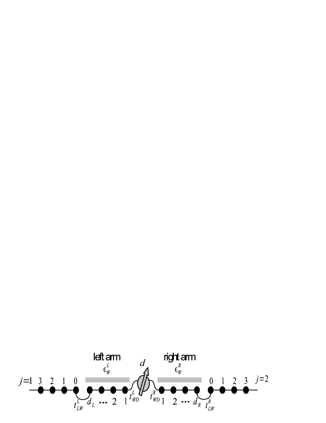
models the Fermi liquid leads as semi-infinite nearest-neighbor tight-binding chains with hopping , where is the lead index and is the site index. For simplicity all leads are assumed to be identical, and we temporarily suppress the spin index. is the non-interacting part of the junction; it glues all leads together and often includes additional sites (e.g. representing the arms of an ABK ring), but does not include coupling to the interacting QD. In a typical open ABK ring with electron leakage, two of the leads serve as source and drain electrodes, while the remaining leads mimic the base contacts thorough which electrons escape the junction. In experiments usually the current flowing through the source or the drain is monitored, but the leakage current can also be measured.
Assume that there are sites in the junction to which the QD is directly coupled; hereafter we refer to these sites as the coupling sites. The coupling to the QD can be written as
| (1d) |
where annihilates an electron on the QD, and creates an electron on the th coupling site. may coincide with . In the simplest AB ring, there is only one physical AB phase, which may be incorporated in either or . In more complicated models both and can depend on AB phases.
Finally, the Hamiltonian of the interacting QD is given by
| (1e) |
where . We assume spin symmetry throughout the paper.
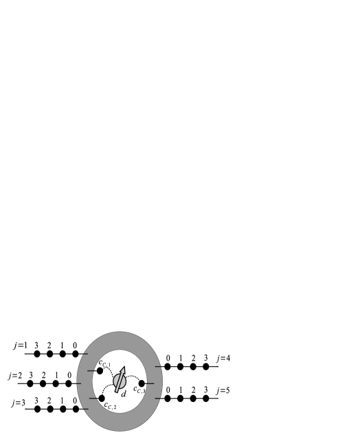
A generic system with and is sketched in Fig. 1, with details of the mesoscopic junction hidden. We will analyze more concrete examples in Secs. V and VI; additional examples, previously studied in Refs. Malecki and Affleck, 2010; Komijani et al., 2013; Simon and Affleck, 2002, are provided in Appendix A.
II.1 Screening and non-screening channels
While it is that ultimately determines the properties of the junction, its details are actually not important in our formalism. Instead, in the following we characterize the model by its background scattering S-matrix and coupling site wave functions. Both quantities are easily obtained from a given , and as we show in Sec. III, they play a central role in our quest for the linear DC conductance.
To recast our model into the standard form of an interacting QD coupled to a continuum of states, it is convenient to first diagonalize the non-interacting part of the Hamiltonian by introducing the scattering basis :
| (2) |
where is the dispersion relation in the leads, and for simplicity we let the lattice constant . In addition to the scattering states , there may exist a number of bound states with their energies outside of the continuum, but since their wave functions decay exponentially away from the junction region, they do not affect linear DC transport properties.
The scattering basis operator annihilates a scattering state electron incident from lead with momentum , and obeys the anti-commutation relation . The corresponding wave function has the following form on site in lead ,
| (3a) | |||
| and on coupling site , | |||
| (3b) |
In other words, for an electron incident from lead , is the background reflection or transmission amplitude in lead , and is the wave function on coupling site . The scattering S-matrix is unitary: .
From its wave function, can be related to and :
| (4a) | |||
| and | |||
| (4b) |
We now express in the scattering basis. Inserting Eq. (4b) into Eq. (1d), we find the QD is only coupled to one channel in the continuum, i.e. the screening channel:
| (5) |
where the screening channel operator is defined by
| (6) |
and the normalization factor is defined by
| (7) |
This ensures . Here we also introduce the Hermitian QD coupling matrix ,
| (8) |
It will be useful to define a series of non-screening channels orthogonal to , where , , . The channels are decoupled from the QD. In a compact notation we can write the transformation from the scattering basis to the screening–non-screening basis as
| (9) |
where is a unitary matrix. The first row of is known:
| (10) |
As long as stays unitary, its remaining matrix elements can be chosen freely without affecting physical observables. now also diagonalizes ,
| (11) |
we shall also need the inverse transformation,
| (12) |
II.2 Kondo model
In the local moment regime of the Anderson model,Kondo (1964); Hewson (1997) for we can perform the Schrieffer-Wolff transformationSchrieffer and Wolff (1966) on to obtain an effective Kondo model with a reduced bandwidth and a momentum-dependent coupling:
| (13a) | |||
| where all momenta are between and with Fermi wave vector , is the initial momentum cutoff, and the dispersion is linearized near the Fermi energy as . For the tight-binding model . | |||
The interaction consists of a spin-flip term ,
| (13b) |
| (13c) |
and a particle-hole symmetry breaking potential scattering term ,
| (13d) |
| (13e) |
The energy cutoff is initially . When we reduce the running energy cutoff from to () to integrate out the high-energy degrees of freedom in the narrow strips of energy and , is exactly marginal in the renormalization group (RG) sense, whereas is marginally relevant and obeys the following RG equation:
| (14) |
or equivalently
| (15) |
where is the density of states per channel per spin, . Therefore, renormalization of the Kondo coupling is controlled by the momentum-dependent normalization factor , defined in Eq. (7). is the only truly independently renormalized coupling constant despite the appearance of Eq. (14); this follows from the fact that the screening channel is the only channel coupled to the QD.Simon and Affleck (2002)
The prototype Kondo model possesses a momentum-independent coupling function, . As a result, spin-charge separation occurs and the Kondo interaction is found to be exclusively in the spin sector.Affleck and Ludwig (1993) The charge sector is nothing but a non-interacting theory with a particle-hole symmetry breaking phase shift due to the potential scattering term , while at very low energy scales the spin sector renormalizes to a local Fermi liquid theory with phase shift.
On the other hand, in a mesoscopic geometry often exhibit fluctuations on a mesoscopic energy scale . (More precisely, can be defined as the energy corresponding to the largest Fourier component in the spectrum of , but for both specific models discussed in this paper we can simply read it off the analytic expression.) In the presence of a characteristic length scale , may be of the order of the Thouless energy , as is the case for the closed long ABK ring in Sec. V; however this is not always true, with a counterexample provided by the open long ABK ring in Sec. VI where is of the order of the bandwidth . Well above , appears featureless and can be approximated by its mean value with respect to . The Kondo temperature can be loosely defined as the energy cutoff at which the dimensionless coupling becomes . As briefly sketched in Sec. I, there are two very different parameter regimes of the Kondo temperature:Simon and Affleck (2002); Yoshii and Eto (2011)
a) The small Kondo cloud regime . For , the size of the Kondo screening cloud ; hence the name. In this regime, the bare Kondo coupling is sufficiently large, so that renormalizes to before it “senses” any mesoscopic fluctuation. By approximating , Eq. (15) has a solution
| (16) |
where is the bare Kondo coupling constant at the initial energy cutoff . Eq. (16) gives the “background” Kondo temperature
| (17) |
independent of the mesoscopic details of the geometry. For , the low-energy effective theory is also conjectured to be a Fermi liquid, but the T-matrix (or the phase shift) of the screening channel is not yet known with certainty.Simon and Affleck (2002); Liu et al. (2012a)
b) The very large Kondo cloud regime . For , . In this regime, the bare Kondo coupling is very small, and does not begin to renormalize significantly until the energy cutoff is well below . The variation of is hence negligible in the resulting low energy theory, , but may be significantly different from , which means Kondo temperature is thus highly sensitive to the mesoscopic details of . Because is almost independent of , we may map the low-energy theory in question onto the conventional Kondo model, where conduction electrons are scattered by a point-like spin in real space. (We stress that this mapping would not be possible for a strongly -dependent , which is the case for the small cloud regime.) Following well-known results in the conventional Kondo model,Hewson (1997) we see that the low-energy effective theory is a local Fermi liquid theory, with parameters also sensitive to mesoscopic details.
III Linear DC conductance
In this section we calculate the DC conductance tensor of the system in linear response theory, generalizing the results in Ref. Komijani et al., 2013 to our multi-terminal setup. The result is presented as the sum of a disconnected contribution and a connected one (Fig. 2). By “disconnected” and “connected”, we are referring to the topology of the corresponding Feynman diagrams: a disconnected contribution originates from a Feynman diagram without any cross-links, and can always be written as the product of two two-point functions. The disconnected contribution has a simple Landauer form, and is quadratic in the T-matrix of the screening channel . The connected contribution is also shown to depend on properties near the Fermi surface only, but it is usually difficult to evaluate analytically except at high temperatures, or at low temperatures if the Fermi-liquid perturbation theory is applicable. Nevertheless, just as with the short ABK ring, the connected contribution can be approximately eliminated at temperatures low compared to another mesoscopic energy scale .

III.1 Kubo formula in terms of screening and non-screening channels
The linear DC conductance tensor is defined through , where is the current operator in lead , and is the applied bias voltage on lead . is given by , where is the real time variable, and
| (18) |
is the density operator in lead . is then given by the Kubo formula
| (19) |
where the retarded density-density correlation function is
| (20) |
and . The retarded correlation function can be obtained by means of analytic continuation from its imaginary time counterpart,
| (21) |
where is a bosonic Matsubara frequency, is the inverse temperature, and is the imaginary time-ordering operator.
To calculate the correlation function we need the density operator written as bilinears of . This is achieved by the insertion of Eq. (4a) and then Eq. (12) into Eq. (18). We find
| (22) |
where for , , …, ,
| (23) |
The matrix obeys which ensures is Hermitian.
III.2 Disconnected part
We substitute Eq. (22) into Eq. (20). The disconnected part of the conductance is obtained by pairing up and operators to form two two-point Green’s functions:
| (24) |
Here the factor of in the second line is due to the spin degeneracy. The greater and lesser Green’s functions in the screening–non-screening basis are defined as
| (25a) | |||
| and | |||
| (25b) |
In equilibrium, fluctuation-dissipation theorem requires that , and , where is the Fermi function. These equilibrium relations result from the fact that for the Anderson model [see Eq. (29) below].Komijani et al. (2013) With these relations Eq. (24) becomes
| (26) |
We note that, in contrast to the case of Ref. Komijani et al., 2013, the momentum integral here is not necessarily real. Instead, its complex conjugate takes the same form but with and interchanged:
| (27) |
Making use of this property, we can show that . Thus the disconnected contribution to the DC conductance can be written as
| (28) |
We should realize, however, that taking the imaginary part of is generally not equivalent to taking the -function part of in Eq. (26).
For the Anderson model, it is not difficult to find the Dyson’s equation for the retarded Green’s function by the equation-of-motion technique:
| (29) |
where the free retarded Green’s function for and is
| (30) |
and is the projection operator onto the screening channel subspace. Again, only the Green’s function of the screening channel is modified by coupling to the QD. The retarded T-matrix of the screening channel in the single-particle sector is related to the retarded two-point function of the QD by
| (31) |
where .
From Eqs. (26) and (29) we may express the disconnected contribution to the linear DC conductance in the Landauer form:
| (32) |
where the disconnected “transmission probability” is written in terms of the absolute square of a “transmission amplitude”,
| (33) | |||||
Again is the QD coupling matrix defined in Eq. (8) and is the density of states per channel per spin for the tight-binding model
| (34) |
The detailed derivation of Eq. (33) by contour methods is left for Appendix B. As a consistency check, we show in Appendix C that for a non-interacting QD, , Eq. (33) and solving the Schroedinger’s equation yield the same transmission probability.
At zero temperature, when the single-particle sector of the screening channel T-matrix obeys the optical theorem and the inelastic part of the T-matrix vanishes,Zaránd et al. (2004) there is no connected contribution and Eq. (32) yields the full linear DC conductance.Komijani et al. (2013) In this case a clear picture emerges from Eq. (33): the conductance is given by the Landauer formula with an effective single-particle S-matrix, which is obtained from the original S-matrix simply by imposing a phase shift on the screening channel, corresponding to the particle-hole symmetry breaking potential scattering and the elastic scattering by the Kondo singlet.Ng and Lee (1988); Malecki and Affleck (2010)
Another useful representation of the disconnected probability, similar to that in Ref. Komijani et al., 2013, is obtained by expanding Eq. (33):
| (35a) | |||||
| with a background transmission term | |||||
| (35b) |
a term linear in the real part of the T-matrix, proportional to
| (35c) |
a term linear in the imaginary part, proportional to
| (35d) |
and a term quadratic in the T-matrix, proportional to
| (35e) |
In the DC limit, the total current flowing out of the junction is zero, and a uniform voltage applied to all leads does not result in any current; hence the linear DC conductance satisfies current and voltage Kirchhoff’s laws . As a comparison it is interesting to consider the sum of the disconnected transmission probability, Eq. (35a), over or . Using the unitarity of and Eq. (8) it is not difficult to find that
| (36) |
and
| (37) |
As mentioned in Ref. Komijani et al., 2013, the quantity in curly brackets in Eqs. (36) and (37) measures the deviation of the single-particle sector of the T-matrix from the optical theorem.Zaránd et al. (2004) In the case of a non-interacting QD or the Fermi liquid theory of the Kondo limit, where the connected contribution to the conductance vanishes, these row/column sum formulas conform to our expectations: the T-matrix obeys the optical theorem, leading to , so that is ensured.
III.3 Connected part and its low-temperature elimination
In this subsection we show that the connected contribution to the conductance is again a Fermi surface contribution, and discuss how it can be approximately eliminated at low temperatures. Following Ref. Komijani et al., 2013 we construct a transmission probability for this contribution. After a partial insertion of Eq. (22) into Eq. (21), the connected part of the density-density correlation function can be written as
| (38) |
where the connected four-point function with two temporal arguments is
| (39) |
the subscript denotes connected diagrams. Note that only the screening channel contributes to the connected part, as the non-screening channels are free fermions. Using the equation-of-motion technique, it is easy to relate to a partially amputated quantity:
| (40) |
where
| (41) |
is the imaginary time free Green’s function and is the Heaviside unit-step function. With only appearing in free propagators, we can perform the Fourier transform explicitly,
| (42) |
One may now use the contour integration argument in Ref. Komijani et al., 2013.Mahan (2000) The final result is that the connected contribution to the DC conductance is expressed in terms of a transmission probability related to :
| (43) |
where
| (44) |
and
| (45) |
Here , are positive infinitesimal numbers.
| (46) |
Here domains of the momentum integrals are extended to according to Eq. (133), which facilitates the application of the residue method. As explained in Appendix B, the poles of and are not important in the DC limit . Therefore, the contribution is dominated by the poles of the free Green’s functions, and is given by
| (47) |
where , , . This leads to
| (48) |
A similar manipulation can be done for the part of the correlation function.
One can again consider the row and column sums of the tensor . Tracing over immediately yields
| (49) |
combining the last two equations, we have
| (50) |
Let us now define as the characteristic energy scale below which both and vary slowly. By definition ; while is not necessarily the same as , for the two ABK ring geometries considered in this paper . For a mesoscopic structure with characteristic length scale , is usually the Thouless energy, ; however, this is again not always the case, and the open long ABK ring in Sec. VI provides a counterexample where is comparable to the bandwidth. Below , the function is only weakly dependent on .
Eq. (50) suggests that we can approximately eliminate the connected part of , provided the temperature is low compared to .Komijani et al. (2013) Consider the linear combination
| (51) |
this corresponds to measuring the conductance by measuring the current in lead , plus a constant times the total current in all leads. (Note that here we include both disconnected and connected contributions.) By Kirchhoff’s law, this linear combination must equal itself. We write it as a sum of disconnected and connected contributions:
| (52) | |||||
For , by Eq. (50), the quantity in curly brackets approximately vanishes for , whereas the Fermi factor approximately vanishes for . Therefore
| (53) |
in other words, at it is possible to write the conductance in terms of disconnected contributions alone.
Since Eq. (53) contains only the disconnected contribution, we may calculate it explicitly using Eqs. (35a) and (36). Since both and are slowly varying below the energy scale , we find the conductance is approximately linear in the T-matrix,
| (54) | |||||
provided . Eq. (54) can also be obtained by eliminating the connected part with the column sum Eq. (37) instead of the row sum,
| (55) |
which corresponds to measuring the conductance by applying a small uniform bias voltage in all leads, in addition to the small bias voltage in lead .
Eq. (54) is the first central result of this paper. It generalizes the result of the two-lead short ABK ring in Ref. Komijani et al., 2013 to an arbitrary ABK ring, and expresses the linear DC conductance as a linear function of the scattering channel T-matrix, as long as the temperature is low compared to the mesoscopic energy scale at which and varies significantly.
IV Perturbation theories
IV.1 Weak-coupling perturbation theory
Although we now understand that the connected part of the conductance can be eliminated at low temperatures, this procedure may not be applicable in the weak-coupling regime . In this subsection we calculate the linear DC conductance perturbatively in powers of , again generalizing the short ring results of Ref. Komijani et al., 2013; we expect the result to be valid in both small and large Kondo cloud regimes as long as and the renormalized Kondo coupling constant remains weak.
IV.1.1 Disconnected part
We first find the disconnected part; the result is already given in Ref. Komijani et al., 2013, but for completeness we reproduce it here. As implied by Eq. (33), our task amounts to calculating the retarded T-matrix of the screening channel in the single-particle sector, which is in turn achieved by calculating the two-point Green’s function . The pertinent Feynman diagrams to and are depicted in Fig. 3, and we find
| (56) |
where again for the model with a reduced band. The factor of results from time-ordering and tracing over the impurity spin, where we have used the following identity
| (57) |

The and terms, accounting for the particle-hole symmetry breaking potential scattering due to the QD, clearly obey the optical theorem . If is comparable to the renormalized value of then the term dominates the T-matrix.
On the other hand, if we tune the QD to be particle-hole symmetric, and , both terms containing will vanish, and the term becomes the lowest order contribution to the T-matrix. For this term, one should also make a distinction between the real principal value part and the imaginary -function part. As noticed in Ref. Malecki and Affleck, 2010 and reiterated in Ref. Komijani et al., 2013, the principal value part introduces non-universalities due to its dependence on all energies in the reduced band ; nevertheless it is merely an elastic potential scattering term, and we neglect it in the following. Meanwhile, the -function part is an inelastic effect stemming from the Kondo physics, as can be seen from its violation of the optical theorem. (The T-matrix apparently disobeys the optical theorem because it is restricted to the single-particle sector, and the sum over intermediate states excludes many-particle states.) Therefore, for a particle-hole symmetric QD, to we haveKomijani et al. (2013)
| (58) |
The weak-coupling perturbation theory is famous for being infrared divergent at ,Kondo (1964); Mahan (2000) but as long as , to logarithmic accuracy we can verify that the corrections to the T-matrix can be absorbed into our result by reinterpreting the bare Kondo coupling constant as a renormalized one. The renormalization is governed by Eq. (14), and cut off at either the “electron energy” or the temperature , whichever is larger. In other words, the Kondo coupling in Eq. (58) should be replaced by , where the argument in round brackets stands for the energy cutoff in Eq. (14) where the running coupling constant is evaluated.
IV.1.2 Connected part
We now calculate the connected part to ; the calculation follows Ref. Komijani et al., 2013 closely. Inserting Eq. (22) into Eq. (21), we write the connected part of the density-density correlation function in terms of a four-point correlation function of :
| (59) |
where
| (60) |
We insert Eqs. (10) and (23) into Eq. (59), and take the continuum limit, which is appropriate for the Kondo model. Because in the wide band limit the most divergent contribution to is from and , we can expand the integrand around these points,
| (61) |
The only non-vanishing diagrams at are shown in panel c) of Fig. 3:
| (62) | |||||
we have again used Eq. (57). The frequency summation is performed by deforming the complex plane contour and wrapping it around the lines and . Analytic continuation yields
| (63) |
Substituting Eqs. (63) and (13b) into Eq. (61), we are able to evaluate the momentum integrals in the limit by contour methods. The and terms vanish, and the terms combine to produce a Fermi surface factor :
| (64) |
where we used Eq. (35e). The connected contribution to the conductance is now clearly a Fermi surface property:
| (65) |
where the connected transmission probability is
| (66) |
This is formally identical to the short ring result, and is of the same order of magnitude [] as the disconnected contribution for a particle-hole symmetric QD.Komijani et al. (2013) In fact, if leads and are not directly coupled to each other (i.e. they become decoupled when their couplings with the QD are turned off; the simplest example is a QD embedded between source and drain leads)Pustilnik and Glazman (2004), we have , and the disconnected contribution for a particle-hole symmetric QD is . In this case the connected contribution dominates.
IV.1.3 Total conductance
We write the total conductance at as a background term and a correction due to the QD:
| (67) |
If the QD is well away from particle-hole symmetry, can be of the same order of magnitude as even when the latter is fully renormalized to the given temperature. In this case, the correction to the background conductance will be dominated by the potential scattering term; the connected contribution is negligible. The expression for is
| (68) |
If, however, the QD is particle-hole symmetric, the connected contribution becomes important. Inserting Eq. (58) into Eq. (35a) and combining with (66), we find the Kondo-type correction to at
| (69) |
Again, in the RG improved perturbation theory, in Eq. (69) should be replaced by , indicating that is the renormalized value at the running energy cutoff . This expression is valid as long as , irrespective of whether the system is in small or large Kondo cloud regime.
Eq. (69) is formally similar to the previously obtained short ring result.Komijani et al. (2013) It should be noted, however, that the energy dependence of , and is possibly much stronger than the short ring case, and the thermal averaging in Eq. (67) can lead to very different results in small and large Kondo cloud regimes. For instance, if (which may happen in the small cloud regime), the Fermi factor in Eq. (67) averages over many peaks in , , and that are associated with the underlying mesoscopic structure. In this case connected part elimination is not applicable. On the other hand, if , the variation of , , or is negligible on the scale of , and the Fermi factor in Eq. (67) may be approximated by a function. This leads to
| (70) |
which agrees with our prescription of eliminating the connected part, Eq. (54).
IV.2 Fermi liquid perturbation theory
It is also interesting to consider temperatures low compared to the Kondo temperature . Since our formalism does not by itself provide a low-energy effective theory of the small cloud regime for , we focus on the very large Kondo cloud regime , where as explained in Sec. II the low-energy effective theory is simply a Fermi liquid theory. If we further assume , then we can simply eliminate the connected contribution to the conductance with Eq. (54).
To use Eq. (54) we need the low-energy T-matrix for the screening channel in the single-particle sector in the Fermi liquid regime, which is again well known.Affleck and Ludwig (1993); Affleck et al. (2008) As mentioned in Sec. I, the strong-coupling single particle wave function at zero temperature is obtained by imposing a phase shift on the weak-coupling wave function. This phase shift results from both elastic scattering off the Kondo singlet and particle-hole symmetry breaking potential scattering:
| (71) |
where for spin-up/spin-down electrons. To the lowest order in potential scattering , we haveMalecki and Affleck (2010)
| (72) |
Let us introduce the phase-shifted screening channel , which is then related to the original screening channel via a scattering basis transformation:
| (73) |
Using the definition of the T-matrix in the single-particle sector Eq. (29) and the transformation Eq. (73) one can show that retarded T-matrices for and are related by
| (74) |
Since diagonalizes the strong-coupling fixed point Hamiltonian, by definition T̃ at zero temperature.
The leading irrelevant operator perturbing the strong-coupling fixed point is localized at the QD (with a spatial extent of ), and quadratic in spin current.Affleck and Ludwig (1993); Glazman and Pustilnik (2005) It is most conveniently written in terms of :
| (75) | |||||
Here denotes normal ordering, and sums over repeated spin indices and are implied. The operators has been unfolded, so that their wave functions are now defined on the entire real axis instead of the positive real axis. The two terms in are illustrated in panel a) of Fig. 4 as a four-point vertex and a two-point one. Both terms share a single coupling constant of , because the leading irrelevant operator written in the basis must be particle-hole symmetric by definition. The on-shell retarded T-matrix for in the single-particle sector is calculated to in Ref. Affleck and Ludwig, 1993:
| (76) |
For completeness we give a derivation of this result in Appendix D. It is diagramatically represented by Fig. 4 panel b).

Substituting Eqs. (71), (74) and (76) into Eq. (54), we eliminate the connected contribution, and obtain the conductance in the very large Kondo cloud regime:
| (77) | |||||
We note that the connected contribution can in fact be evaluated directly in the Fermi liquid theory. This is also done in Appendix D, and provides further verification of our scheme of eliminating the connected contribution.
Predictions of the conductance at high temperatures [Eq. (67)] and at low temperatures [Eq. (77)] together constitute the second main result of this paper. We emphasize once more that, while Eq. (67) is valid as long as , Eq. (77) is expected to be justified provided , so that the Fermi liquid theory applies, and also , so that the connected contribution can be eliminated.
For clarity we tabulate various regimes of energy scales discussed so far (Table 1). Note again that the connected contribution to conductance can be eliminated when . In general we have , but we assume in this table that , which is the case with the systems to be discussed in this paper.
| Weak-coupling perturbation theory applies | depends on mesoscopic details | Connected part elimination possible | |
| Yes | No | No | |
| Yes | Yes | No | |
| Yes | Yes | Yes |
| Fermi liquid perturbation theory applies | depends on mesoscopic details | Connected part elimination possible | |
| Yes | Yes | Yes | |
| ? | No | Yes | |
| ? | No | No |
V Closed long ABK rings
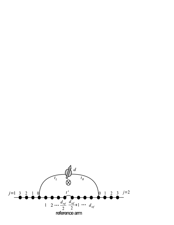
In this section we apply our general formalism to the simplest model of a closed long ABK ring, studied in Ref. Yoshii and Eto, 2011 (Fig. 5): the QD is coupled directly to the source and drain leads, and a long reference arm connects the two leads smoothly. A weak link with hopping splits the reference arm into two halves of equal length where is an even integer. As opposed to Ref. Yoshii and Eto, 2011, however, we use gauge invariance to assign the AB phase to the QD tunnel couplings rather than the weak link: and . We assume no additional non-interacting long arms connecting the QD with the source and drain leads, because multiple traversal processes in such long QD arms will lead to interference effectsMiroshnichenko et al. (2010) independent of the AB phase, complicating the problem.Yoshii and Eto (2011) The Hamiltonian representing this model takes the form
| (78) | |||||
the coupling sites are and .
We first repeat the Kondo temperature analysis in Ref. Yoshii and Eto, 2011 in order to distinguish between small and large Kondo cloud regimes, then carefully study the conductance at high and low temperatures, taking into account the previously neglected connected contribution.
V.1 Kondo temperature
The background S-matrix for this model is identical to the short ABK ringMalecki and Affleck (2010) up to overall phases, due to the smooth connection between reference arm and leads:
| (79) |
where the S-matrix elements and for the weak link are
| (80) |
and we introduce the shorthand . The wave function is also straightforward to find:
| (81) |
In the wide band limit, and are approximately independent of in the reduced band where the momentum cutoff . This allows us to approximate them by their Fermi surface values, and (the phase difference is required by unitarity of ); without loss of generality we focus on the case.
From Eq. (81) one conveniently obtains the normalization factor
| (82) | |||||
where measures the degree of symmetry of coupling to the QD. In the second line we have used and introduced another phase , where is a function of , and but independent of . We note that this expression is also applicable in the continuum limit, where the lattice constant (we have previously set ) but the arm length is fixed. In that case should be understood as the arm length .
For long rings and filling factors not too small , oscillates around as a function of , and has its extrema at where takes integer values. The only characteristic energy scale for is therefore the peak/valley spacing , and . As in Ref. Yoshii and Eto, 2011 we define the reduced band such that , and the reduced band initially contains many oscillations.
In the small Kondo cloud regime , one may assume the oscillations of are smeared out when the energy cutoff is being reduced from , which is still well above : . This means in this regime is approximately the background Kondo temperature defined in Eq. (17), independent of the position of the Fermi level at the energy scale , and also independent of the magnetic flux.
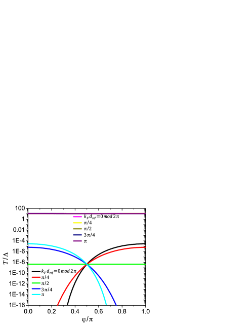
On the other hand, in the large cloud regime , now that the Kondo temperature is largely determined by the value of in a very narrow range of energies around the Fermi level, the mesoscopic oscillations become much more important. When the running energy cutoff is above the peak/valley spacing , the renormalization of is controlled by as in Eq. (16). Once is reduced below , we may approximate the renormalization of as being dominated by . This leads to the following estimation of the Kondo temperature:
| (83) |
It is clear that can be significantly dependent on the AB phase in this regime. In particular, varies from (“on resonance”) to practically (“off resonance”) as is tuned between and , when the Fermi energy is located on a peak or in a valley , the background transmission is perfect , and coupling to the QD is symmetric ; see Fig. 6.Yoshii and Eto (2011) (The special case corresponds to a pseudogap problem , and the stable RG fixed point can be the local moment fixed point or the asymmetric strong coupling fixed point, depending on the degree of particle-hole symmetry.Vojta and Fritz (2004); *PhysRevB.70.214427) As a general rule, stronger transmission through the pinch and greater symmetry of coupling result in stronger interference between the two tunneling paths through the device, and hence increases the tunability of the Kondo temperature by the magnetic flux.
V.2 High-temperature conductance
We now calculate the conductance at by perturbation theory. Following the discussion in Ref. Yoshii and Eto, 2011, we consider the case of a particle-hole symmetric QD and , and also ignore the elastic real part of the potential scattering generated at .Komijani et al. (2013) These assumptions allow us to adopt Eq. (69) for the correction to the transmission probability:
Note that Eq. (84) does not depend on details of the non-interacting part of the ring Hamiltonian . For a parity-symmetric geometry with two leads and two coupling sites (), when coupling to the QD is also symmetric () and time-reversal symmetry is present ( or ), we can further show that the sign of the transmission probability correction is determined by the sign of , a property discussed in Ref. Komijani et al., 2013 at the end of Sec. IV C. Indeed, parity symmetry implies that , , , ; hence it is not difficult to find from Eq. (84) that
| (85) |
The left-hand side correspond to a particular way to measure the conductance, namely parity-symmetric bias voltage and parity-symmetric current probes, or in Sec. V of Ref. Komijani et al., 2013.
We now return to the long ring geometry without assumptions about , and . Plugging Eqs. (79) and (81) into Eq. (84) we find
| (86) |
where the coefficients , and are independent of but are usually complicated functions of :
| (87a) | ||||
| (87b) |
| (87c) |
In the special case of a smooth reference arm and , the Kondo-type correction becomes especially simple:
| (88) |
As in Refs. Yoshii and Eto, 2011; Komijani et al., 2013, only the first and the second harmonics of the AB phase appear in the correction to the transmission probability .
We may perform the thermal averaging in Eq. (67) at this stage. The Fermi factor ensures only the energy range contributes significantly to the conductance; in this energy range the renormalization of is cut off by .
In the small Kondo cloud regime, means so that we can average over many peaks of , so we may drop all rapidly oscillating Fourier components in Eq. (86). This leads to
| (89) |
We see that the first harmonic in approximately drops out upon thermal averaging.
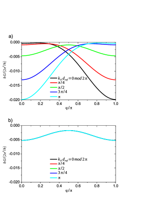
On the other hand, in the large Kondo cloud regime, for it is possible to have either or . In the former case Eq. (89) continues to hold. In the latter case has little variation in the energy range , so it is appropriate to replace with a function at the Fermi level; thus
| (90) |
Fig. 7 illustrates these two different cases for the large Kondo cloud regime. We note that our results, Eq. (89) for and Eq. (90) for , are different from those of Ref. Yoshii and Eto, 2011. We believe the discrepancy is due to the fact that only single-particle scattering processes are taken into consideration by Ref. Yoshii and Eto, 2011; the connected contribution to the conductance is omitted, despite being of comparable magnitude with the disconnected contribution.
V.3 Fermi liquid conductance
It is also interesting to calculate the conductance in the limit in the very large Kondo cloud regime, starting from Eq. (77). We make the assumption that the particle-hole symmetry breaking potential scattering is negligible, , as in Ref. Yoshii and Eto, 2011. Inserting Eqs. (79) and (81) into Eqs. (35d) and (35e), we find the total conductance has the form
| (91) |
where the transmission probability is
| (92) |
While Eq. (91) is ostensibly in agreement with Eq. (69) of Ref. Yoshii and Eto, 2011, we suspect that there are two oversights in the derivation of the latter: at finite temperature, Ref. Yoshii and Eto, 2011 neglects the connected contribution to the conductance, and also replaces the thermal factor with a function in Eq. (54). These two discrepancies cancel each other, leading to the same result as ours.
VI Open long ABK rings
We turn to the open long ABK ring, with strong electron leakage due to side leads coupled to the arms of the ring, where our multi-terminal formalism shows its full capacity.
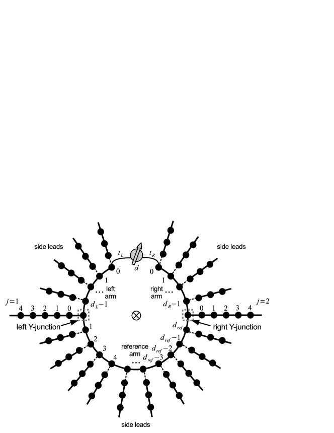
In our geometry shown in Fig. 8, the source lead branches into two paths at the left Y-junction, a QD path of length and a reference path of length . These two paths converge at the right Y-junction at the end of the drain lead. An embedded QD in the Kondo regime separates the QD path into two arms of lengths and . To open up the ring we attach additional non-interacting side leads to all sites inside the ring other than the two central sites in the Y-junctions and QD.Aharony et al. (2002); Aharony and Entin-Wohlman (2005); Simon et al. (2005); Carmi et al. (2012) The side leads, numbering in total, are assumed to be identical to the main leads (source and drain), except that the first link on every side lead (connecting site of the side lead to its base site in the ring) is assumed to have a hopping strength which is generally different than the bulk hopping . The Hamiltonian representing this model is therefore
| (93) | |||||
where is the annihilation operator on the central site of the left (right) Y-junction, and is the annihilation operator on site of the side lead attached to the th site on arm , , and . The coupling sites are and , and again we let the couplings to the QD be and .
Our hope is that in certain parameter regimes the open long ring provides a realization of the two-path interferometer, where the two-slit interference formula applys:
| (94) |
where is the conductance through the reference arm with the QD arm sealed off, and is the conductance through the QD with the reference arm sealed off. is as before the AB phase, and is the accumulated non-magnetic phase difference of the two paths (including the transmission phase through the QD). is the unit-normalized visibility of the AB oscillations; at zero temperature if all transport processes are coherent.Carmi et al. (2012) In the two-path interferometer regime, reflects the intrinsic transmission phase through the QD, provided that the geometric phases of the two paths are the same (e.g. identical path lengths in a continuum model), no external magnetic field is applied to the QD, and the particle-hole symmetry breaking phase shift is zero.
For non-interacting embedded QDs well outside of the Kondo regime, small transmission through the lossy arms is known to suppress multiple traversals of the ring and ensure that the transmission amplitudes in two paths are mutually independent.Aharony et al. (2002) We show below that in our interferometer with a Kondo QD, the same criterion renders the mesoscopic fluctuations of the normalization factor negligible, and paves the way to the two-slit condition . If we additionally have small reflection by the lossy arms, then both the Kondo temperature of the system and the intrinsic transmission amplitude through the QD are the same as their counterparts for a QD directly embedded between the source and the drain. At finite temperature , we recover and generalize the single-channel Kondo results of Ref. Carmi et al., 2012 for the normalized visibility and the transmission phase .
VI.1 Wave function on a single lossy arm
To solve for the background S-matrix and the wave function matrix of the open ring, we first analyze a single lossy arm attached to side leads, depicted in Fig. 9.Aharony et al. (2002)

Consider an arbitrary site labeled on this arm; let the wave function on this site be , and let incident and scattered amplitudes on the side lead attached to this site be and . The wave function on site () on the side lead is then written as . The Schroedinger’s equations are
| (95a) |
| (95b) |
Eliminating , we find
| (96) |
This means if , i.e. no electron is incident from the side lead , we can write the wave function on the th site on the arm as
| (97) |
where are constants independent of and . are roots of the characteristic equation
| (98) |
so that . Hereafter we choose the convention . When , to the lowest nontrivial order in ,
| (99) |
and thus .
Eq. (97) bypasses the difficulty of solving for each individually: on the same arm the constants and only change where the side lead incident amplitude .
Let us now quantify the conditions of small transmission and small reflection. Connecting external leads smoothly to both ends of a lossy arm of length , we may write the scattering state wave function incident from one end as
| (100) |
the Schroedinger’s equation then yields
| (101a) |
| (101b) |
| (101c) |
| (101d) |
It is now straightforward to find the transmission and reflection coefficients:
| (102a) |
| (102b) |
At or we always have trivially and ; we therefore focus on energies that are not too close to the band edges, so that is not too small. In this case, under the long arm assumption , the small transmission condition is satisfied if and only if , and the small reflection condition is satisfied if and only if .Aharony et al. (2002)
VI.2 Background S-matrix and coupling site wave functions
We now return to the open long ring model to solve for and with the aid of Eq. (97). Let us denote the incident amplitude vector by
| (103) |
here is the incident amplitude in the side lead attached to the th site on arm . We are interested in the normalization factor and the source-lead component of the conductance tensor ; for this purpose, according to Eqs. (7) and (77), the first two rows of the S-matrix and the full coupling site wave function matrix must be found. In other words, we need to express the scattered amplitudes in the main leads , , as well as the wave functions at the coupling sites and , in terms of incident amplitudes. Some details of this straightforward calculation are given in Appendix E, and we skip to the solution now.
If we assume (comparable arm lengths and path lengths in the long ring) and (small transmission criterion), to we have
| (104a) | ||||
| (104b) |
| (104c) |
| (104d) |
Here the matrices and are defined in Eqs. (203) and (204); they are generally not unitary. Being properties of the Y-junctions, they are independent of the amplitudes (, etc.) and arm lengths (, and ), as can be seen from e.g. Eq. (205). In the limit , and turn into the usual unitary S-matrices and .
VI.3 Kondo temperature and conductance
To the lowest nontrivial order in , Eq. (104) leads to the following simple results after some algebra:
| (105) |
| (106) |
| (107) |
In obtaining Eq. (107) we have used the algebraic identity
| (108) |
in the limit this is just a statement of the S-matrix unitarity.
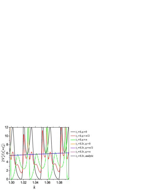
Eq. (105) tells us that, in the small transmission limit, the normalization factor exhibits little mesoscopic fluctuation, so that ; furthermore, it does not depend on the AB phase at all (see Fig. 10). When we also impose the small reflection condition , and we find ; this is precisely the normalization factor for a QD embedded between source and drain leads. We recall from Eq. (15) that the normalization of Kondo coupling is governed by . Therefore, at least for our simple model of an interacting QD, the conditions of small transmission and small reflection combine to reduce the Kondo temperature of the open long ABK ring to that of the simple embedded geometry, independent of the details of the ring or the AB flux.
Proceeding with the small transmission assumption, we observe that since , the distinction between small and large Kondo cloud regimes is no longer applicable. This is presumably because the Kondo cloud leaks into the side leads in the open ring, and is no longer confined in a mesoscopic region as in the closed ring. The low-energy theory of our model is therefore the usual local Fermi liquid. At zero temperature, the connected contribution to the conductance vanishes, and the conductance is proportional to the disconnected transmission probability Eq. (33) at the Fermi energy:
| (109) |
where , and are all evaluated at the Fermi surface, and we have used Eqs. (71) and (74). In the small reflection limit, Eq. (109) becomes
| (110) |
where are the aforementioned S-matrices of the Y-junctions, and
| (111) |
is the transmission amplitude through an embedded QD in the Kondo limit [see Eq. (123)].
It is clear from Eq. (109) that the two-slit condition is satisfied at zero temperature. Furthermore, under the small reflection condition, both and have straightforward physical interpretations; in particular can be factorized into a part which is the intrinsic transmission amplitude through QD, and a part due completely to the rest of the QD arm and the two Y-junctions.
We now consider the finite temperature conductance, assuming realistically that and . If we further assume that the two Y-junctions are non-resonant, so that and change significantly as functions of energy only on the scale of the bandwidth , then mesoscopic fluctuations are entirely absent from Eq. (107), i.e. . (It is worth mentioning that can be much less than if the Y-junctions allow resonances, e.g. when the central site of each Y-junction is weakly coupled to all three legs; however, even in this case.) Since , we can comfortably eliminate the connected contribution and use Eq. (77). At the total Fermi liquid regime conductance is found to :
| (112a) | |||
| Here the conductance through the reference path is defined as | |||
| (112b) |
the conductance through the QD path is defined as
| (112c) |
with its and value
| (112d) |
and finally the non-magnetic phase difference between the QD path and the reference path (including the QD) in the absence of is
| (112e) |
Once again, , and are all evaluated at the Fermi surface.
For , we discuss two different scenarios: the particle-hole symmetric case and the strongly particle-hole asymmetric case. In the particle-hole symmetric case, as explained in Sec. IV, the potential scattering term vanishes, and the connected contribution plays an important role. Inserting Eqs. (105)–(107) into Eqs. (69) and (67), we find the total high-temperature conductance in the particle-hole symmetric case to be
| (113) |
Here the conductance through the reference path is given as before, while the conductance through the QD path has the usual logarithmic temperature dependence,
| (114) |
We have taken into account the renormalization of the Kondo coupling, Eq. (16); thermal averaging cuts off the logarithm at . For our slowly varying given by Eq. (105), is simply the Fermi surface value , and the Kondo temperature is defined by Eq. (17).
Comparing Eqs. (112a) and (113) and noting that , we find that there is no phase shift between and in the presence of particle-hole symmetry, which is consistent with e.g. Fig. 4(d) of Ref. Gerland et al., 2000. We also observe that the particle-hole symmetric normalized visibility , defined in Eq. (94), has a characteristic logarithmic behavior at :
| (115) |
On the other hand, to demonstrate the phase shift due to Kondo physics, it is more useful to consider the case of relatively strong particle-hole asymmetry at . The leading contribution to the conductance from potential scattering is , and the leading contribution from the Kondo coupling is ; therefore, indicates that we may neglect the Kondo coupling altogether at temperature . To the lowest order in potential scattering , Eq. (68) applies; also, since , the thermal averging in Eq. (67) becomes trivial. Using the relation between and , Eq. (72), we finally obtain
| (116) |
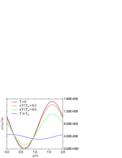
Comparing Eqs. (112a) and (116), it becomes evident that transmission through the QD undergoes a phase shift from to as the Kondo correlations are switched on; see Fig. 11. We remark that the strongly particle-hole asymmetric case represents the situation without Kondo correlation whereas the particle-hole symmetric case does not. This is because in the latter case the leading QD contribution to the conductance is , which is of Kondo origin as we have discussed above Eq. (58).
We can again make a direct comparison with Eq. (94). While itself is not necessarily , is experimentally observed with respect to its value with Kondo correlations turned off, so we should define the reference value by e.g. comparing with Eq. (116):
| (117) |
Therefore, to we readily obtain the following results for the transmission phase and the normalized visibility:
| (118) |
| (119) |
These are in agreement with the , and , results of Ref. Carmi et al., 2012, which assumes , i.e. the non-magnetic phase difference between the two paths is zero without Kondo correlations. Note that in obtaining the dependence in Eq. (119) it is crucial to include the connected contribution to conductance.
We stress that our results for the transmission phase across the QD and the normalized visibility, Eqs. (118) and (119), are both exact in , which is non-universal and encompasses the effects of all particle-hole symmetry breaking perturbation. In particular, the coefficients were not reported previously.
VII Conclusion and open questions
In this paper, we generalized the method developed in Ref. Komijani et al., 2013 to calculate the linear DC conductance tensor of a generic multi-terminal Anderson model with an interacting QD. The linear DC conductance of the system has a disconnected contribution of the Landauer form, and a connected contribution which is also a Fermi surface property. At temperatures low compared to the mesoscopic energy scale below which the background S-matrix and the coupling site wave functions vary slowly, , the connected contribution can be approximately eliminated using properties of the conductance tensor; the elimination procedure physically corresponds to probing the current response or applying the bias voltages in a particular manner. At temperatures high compared to the Kondo temperature this connected part is computed explicitly to , and found to be of the same order of magnitude as the disconnected part in the case of a particle-hole symmetric QD.
With this method we scrutinize both closed and open long ABK ring models. We find modifications to early results on the closed ring with a long reference arm of length : the high-temperature conductance at should have qualitatively distinct behaviors for and . In the open ring we conclude that the two-path interferometer is realized when the arms on the ring have weak transmission and weak reflection, and demonstrate the possibility to observe in this device the phase shift due to Kondo physics, and the suppression of AB oscillation visibility due to inelastic scattering.
One question we have not so far addressed is the low-energy physics in the small Kondo cloud regime, and ; here is the energy scale below which the normalization factor controlling the Kondo temperature varies slowly, and . We assume and are of the same order of magnitude, a condition satisfied by both the closed ring () and the open ring with non-resonant Y-junctions (). For temperatures above the mesoscopic energy scale , we are no longer able to eliminate the connected contribution. However, because one can argue that physics associated with the energy scale is smeared out by thermal fluctuations, and the mesoscopic system behaves as a bulk system with parameters showing no mesoscopic fluctuations.Liu et al. (2012a) On the other hand, below the mesoscopic energy scale , since for our formalism predicts that the connected part can be eliminated, the knowledge of the screening channel T-matrix in the single-particle sector alone is adequate for us to predict the conductance. Ref. Liu et al., 2012a again offers an appealing hypothesis: the low-energy effective theory is again a Fermi liquid theory, with the T-matrix governed by Kondo physics at short range and modulated by mesoscopic fluctuations at long range . This scenario leads to a quasiparticle spectrum which is in qualitative agreement with slave boson mean field theory.Liu et al. (2012a) The Fermi liquid picture is often analyzed by a renormalized perturbation theory of the quasiparticles, where the bare parameters of the QD are replaced by renormalized values; in particular the large between bare electrons is replaced by a small renormalized between quasiparticles.Hewson (1997) In the small Kondo cloud regime, we expect that the real space geometry in the renormalized perturbation theory resembles that of the bare theory;Simon and Affleck (2002) thus a perturbation theory calculation in in our formalism is potentially useful in understanding the low-energy physics, as long as is interpreted as the effective . It will be interesting to test this picture, along with our perturbative predictions on conductance in other parameter regimes in this paper, against results obtained from the numerical RG algorithm.Gerland et al. (2000); Hofstetter et al. (2001); Affleck et al. (2008)
There is also an issue regarding the assumption of a single-level QD in the Kondo regime. To experimentally detect the phase shift in an AB interferometer, one typically sweeps the plunger gate voltage on the QD, and monitors the phase shift between consecutive Coulomb blockade peaks. A plateau should be observed at near the center of each Coulomb valley deep in the local moment regime, with an odd number of electrons on the QD.Gerland et al. (2000); Takada et al. (2014) However, one needs to adopt a multi-level QD model to quantitatively reproduce the experimental results, in particular the phase shift lineshape asymmetry relative to the center of a valley, and also possibly a phase lapse inside the valley.Silvestrov and Imry (2003); Takada et al. (2014) A generalization of the current formalism to the multi-level case is necessary in order to quantify the influence of the interferometer on the measured transmission phase shift through a realistic QD.
Another natural open problem is the extension to the multi-channel Kondo physics. In our generalized Anderson model, separation of screening and non-screening channels is achieved in a single-level QD, and there is only one effective screening channel. Exotic physics emerges in the presence of two or more screening channels, realizable in e.g. a many-QD system.Affleck and Ludwig (1993); Oreg and Goldhaber-Gordon (2003); Potok et al. (2007) In the 2-channel Kondo effect with identical couplings to two channels, for example, the low-energy physics is governed by a non-Fermi liquid RG fixed point: at zero temperature a single particle scattered by the impurity can only enter a many-body state, and there are no elastic single-particle scattering events.Zaránd et al. (2004) Ref. Carmi et al., 2012 discusses the manifestations of the 2-channel Kondo physics in the two-path interferometer, but again makes the two-slit assumption without examining its validity. Therefore an extension of our approach to the multi-channel case will be useful to justify the two-slit assumption in the open long ring and thus the 2-channel predictions of Ref. Carmi et al., 2012.
Acknowledgements.
This work was supported in part by NSERC of Canada, Discovery Grant 36318-2009 (ZS). ZS is grateful to Prof. Ian Affleck for initiating the project, extensive discussions and proofreading the manuscript. YK gratefully acknowledges the kind hospitality of UBC Department of Physics and Astronomy during his visit. The authors would also like to acknowledge fruitful discussions with Prof. L. I. Glazman, as well as valuable comments and suggestions of two anonymous reviewers.Appendix A Comparison with early results
A.1 Short ABK ring
Our formalism can be applied to the short ABK ringMalecki and Affleck (2010); Komijani et al. (2013) shown in Fig. 12. There are two leads () and two coupling sites (); . The coupling sites coincide with the th sites of the leads, , ; also the AB phase is on the couplings to the QD, and . We again let .
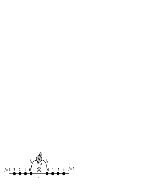
It is straightforward to obtain the background S-matrix and coupling site wave function matrix:
| (120) |
| (121) |
With Eqs. (15), (69) and (77), one reproduces all analytic results in Refs. Malecki and Affleck, 2010; Komijani et al., 2013, including the Kondo temperature, the high- and low-temperature conductance, and the elimination of connected contribution at low temperatures.
The limit is useful as a benchmark against long ring geometries so we study it in some more detail. In this limit we recover the simplest geometry where a QD is embedded between source and drain leads.Pustilnik and Glazman (2004) The normalization factor is
| (122) |
and the zero-temperature transmission amplitude through the QD is given by Eqs. (33), (71), (74) and (76):
| (123) | |||||
A.2 Finite quantum wire
Another special case is the finite wire (or semi-transparent Kondo box) geometry in Fig. 13 where the reference arm is absent;Simon and Affleck (2002) again . The left and right QD arms and coupling sites are subject to gate voltages:
| (124) | |||||
The coupling sites are the first sites of the QD arms, , ; and .
The two leads are decoupled without the QD, so and are both diagonal. In this system we have
| (125) |
and
| (126) |
where is determined by the gate voltage ,
| (127) |
and . and can be obtained simply by substituting with . Again, these results allow us to reproduce the (weak coupling) Kondo temperature, the high-temperature conductance, as well as the low-temperature conductance in the large Kondo cloud regime. (We did not quantitatively discuss the low-temperature conductance in the small cloud regime in this paper; see Sec. VII.)
Appendix B Details of the disconnected contribution
In this appendix we present the detailed derivation of Eq. (33) [or equivalently Eq. (35a)] from Eq. (26). The calculations are similar to those in Appendix B of Ref. Komijani et al., 2013, but an important difference is that here we cannot simply take the -function part and neglect the principal value part in Eq. (26). Instead, most of the momentum integrals are evaluated by means of contour integration.
From Eq. (29)
| (128) |
We denote the three terms above as , and respectively. Inserting into Eq. (26), we find types of contributions to the disconnected part:
| (129) |
The term is the background transmission, the first pair of square brackets is linear in the T-matrix of the screening channel, and the second pair of square brackets is quadratic in the T-matrix.
Due to the multiplying factor of in Eq. (19), terms in contribute to the linear DC conductance, while and other terms which are regular in the DC limit do not contribute. (We can check explicitly that there are no or higher-order divergences.) Therefore, in the DC limit we are only interested in the part of .
B.1 Properties of the S-matrix and the wave functions
Before actually doing the calculations it is useful to examine the properties of the background S-matrix and the wave functions in our tight-binding model, since we rely on these properties to transform the momentum integrals into contour integrals and evaluate them.
First consider the analytic continuation . The wave function “incident” from lead at momentum takes the following form on lead [cf. Eq. (3a)],
| (130) |
and on coupling site ,
This wave function should be a linear combination of the scattering state wave functions at momentum which form a complete basis. The linear coefficients are obtained from S-matrix unitarity:
| (131) |
and the same coefficients apply to the coupling sites:
Hence
| (132) |
Another useful property is the location of poles of on the complex plane. Our analysis closely follows Ref. Perelomov et al., 1998 which deals with the case of quadratic dispersion.
Consider one pole of the S-matrix , where for certain values of and , . In the scattering state , where is the Fermi sea ground state, the incident component of the wave function at momentum becomes negligible relative to the scattered component. Therefore, the time-dependent wave function on lead at site reads
| (134) |
This expression is valid for any where is divergent; for other the wave function is negligible.
We define the “junction area” to include any tight-binding site that is not part of a lead, together with the 0th site of each lead. The total probability of the electron being inside the junction area, , obeys the probability continuity equation
| (135) |
where the right-hand side is the current operator between site and site of lead , summed over all leads. Taking the expectation value in the state , we find
| (136) |
For the left-hand side we have used the form of the time evolution , and is a positive time-independent constant proportional to the total probability in the junction area; is divergent whenever is divergent. For the right-hand side, we have used Eq. (134) at and ; the summation is over any where is divergent.
Eq. (136) implies that either , in which case or ; or , in which case . The poles of on the plane are therefore either outside the unit circle or located on the real axis. For the models we study in this paper, the poles of and those of coincide (see also Sec. C); in other words, the poles of and on the plane are either outside the unit circle or on the real axis.
B.2 Background transmission
This part is independent of the QD and the result should be the famous Landauer formula:
| (138) |
By residue theorem we can perform the integral in the part proportional to and the integral in the part proportional to . In the following we assume ; the case can be dealt with similarly.
We begin from the first term in curly brackets, which is proportional to . For the part proportional to , making the substitution , and calculating the contour integral on the counterclockwise unit circle, we find
| (139a) | |||
| where . ( corresponds to the rate of switching on the bias voltage in Kubo formalism, so the limit should be taken before the DC limit .) We have assumed where if is real; the poles of the integrand inside the unit circle are then and . At the band edges, , and is purely imaginary; we can choose it to have a positive imaginary part so the above expression remains valid. Similarly | |||
| (139b) |
where , if is real, or if is purely imaginary. Now combine the two parts. In the limit, only for real and , and only for real and ; the most divergent contribution is therefore
| (140) |
We have substituted the dummy variables , , and noted that . Expanding various parts of the integrand in limit, we find
| (141) |
The two terms in which are linear in the S-matrix do not contribute any terms of to : the difference of Fermi functions is proportional to , but the denominators are also , unlike the case for the terms whose denominators are . This leaves us with the term quadratic in the S-matrix, which can be similarly evaluated. For the part proportional to ,
| (142a) | |||
| the poles of inside the unit circle (on the real axis) may contribute to the contour integral, but these terms are regular in the limit and do not contribute to the DC conductance. Similarly | |||
| (142b) |
Therefore
| (144) |
taking the limit, noting that , we recover the Landauer formula, Eq. (35b).
B.3 Terms linear in T-matrix
We focus on ; the calculation of is analogous.
| (146a) | |||
| (146b) |
Writing , where or , we are now free to do the and integrals. The poles of and are again not important in the DC limit:
| (147a) | |||
| (147b) |
Now do the and integrals. The terms are regular in the DC limit, so we only need to keep the terms. In the term, while the integral in the part is straightforward, the integral in the part can be simplified by expanding around :
| (148a) | |||
| Here, in the part, we have written () assuming , integrated over using the complex variable , and again neglected contributions from the poles of . Because is always positive and never close to , the denominator for the part is ; thus the part is itself . Meanwhile, in the part, we have used for . We then extend the domain of integration back to the entire real axis. Both and are analytic in the upper half plane; thus, closing the contour above the real axis, the integral in the part sees no pole and vanishes. Similarly, in the term, | |||
B.4 Terms quadratic in T-matrix
We focus on first.
| (150) |
We can integrate over all four momenta. Let where or , and where or ; integrating over and ,
| (151) |
finally, integrating over and , we find
| (152a) |
| (152b) |
Expanding around and integrating over and , assuming , we obtain
| (153) |
where we have written . A similar calculation can be performed on and ; both are for the same reason that is . Therefore, is the only term quadratic in the T-matrix which contributes to the linear DC conductance. Note that this is not the case in Ref. Komijani et al., 2013, where the term and the term are complex conjugates as a result of taking the -function part in Eq. (26). It is easy to see that Eq. (153) reproduces Eq. (35e).
We mention in passing that Eq. (35a) can be derived in the wide band limit with essentially the same method, although the pole structure is much simpler in that case.
Appendix C Non-interacting QD
In this appendix we verify Eq. (33) in the case of a non-interacting QD with as a consistency check on our formalism. The connected part must vanish completely in this case; thus the disconnected contribution to the conductance should coincide with the Landauer formula, with an S-matrix modified by the presence of the non-interacting QD.
C.1 Relation between and
First let us quantify the relation between the background S-matrix and the coupling site wave function matrix . and are both determined by the non-interacting part of the system with the QD decoupled, and are usually intimately related: for instance they often have the same poles on the complex momentum plane, and have resonances (sharp changes in amplitude and phase) over the same range of real momenta. To characterize this relation, we attach to each of the coupling sites an additional “phantom” lead. These phantom leads have the same nearest neighbor hopping as the pre-existing leads. The coupling site is designated as site of its phantom lead. We let be the S-matrix of the resulting non-interacting system with leads; that is, for the scattering state incident from lead with momentum , the wave function on lead should be
| (154) |
and can be , , or , , , so that is an unitary matrix. For future convenience we partition as follows,
| (155) |
where and are shorthands for lead and dot respectively; is and is . Note that and are not usually unitary, although all four blocks are constrained by the overall unitarity of . Also, our argument for in Sec. B applies to :
| (156) |
Due to the non-interacting nature of the system, we can conveniently express and in terms of the auxiliary object . With the QD decoupled, the phantom leads should be terminated by open boundary conditions. The wave function on phantom lead should be
| (157) |
so that and . The incident amplitude and reflected amplitude in lead are respectively . We then see, from the definition of , that and obey the following relations:
| (158a) |
| (158b) |
Therefore,
| (159) |
and
| (160) |
It is straightforward to check the unitarity of .
C.2 Green’s function of the QD
We now find the retarded T-matrix of the non-interacting QD. As is standard for the non-interacting Anderson model in Eq. (5),Mahan (2000) the retarded Green’s function for the QD is
| (161) |
where , and the retarded self-energy is
| (163) |
With contour methods it is straightforward to show, for and integer , that
| (164) |
We now make the assumption that is analytic at the origin of the complex plane. This appears to be a reasonable assumption, because a singularity at the origin would imply an infinite energy feature, which should decouple completely from any properties of system probed at finite energies. Thus can be expanded around the origin in a Taylor series of , and we may integrate term by term to find
| (165) |
where and are non-negative integers.
Expanding in powers of and , the only negative power term in the series is ; therefore, by Eq. (164),
| (166) |
and hence
| (167) |
Eqs. (161) and (167) give the retarded T-matrix T. One can easily verify that the optical theorem is obeyed, which must be the case for a non-interacting system. Inserting Eqs. (160), (159), (161), and (167) into Eq. (33), we find
| (168) |
where
| (169) |
Here we have defined the dimensionless coupling matrix
| (170) |
C.3 Landauer formula
We turn to the alternative method of scattering state wave functions to find the S-matrix in the presence of the QD.
By definition, for the scattering state incident from , the wave function on lead is
| (171) |
The coupling sites are now attached to the QD. We imagine that the QD and the coupling sites are separated by “phantom leads” of zero length, so that the wave function on phantom lead takes the form
| (172) |
where only. Since the phantom leads are also attached to the QD, the Schroedinger equation on coupling site is
| (173) |
where is the wave function on the QD. Meanwhile, the Schroedinger equation on the QD itself is
| (174) |
Eqs. (173) and (174) allow us to express in terms of , i.e. to find the S-matrix for the non-interacting QD:
| (175) |
or more compactly
| (176) |
| (177) |
On the other hand, the amplitudes and are also related to each other and to by the phantom-lead S-matrix :
| (178) |
and
| (180) |
Appendix D Fermi liquid perturbation theory
In this appendix, we discuss the perturbation theory in the Fermi liquid regime (also assuming ; see Table 1). We first present an alternative derivation of Eq. (76), the retarded T-matrix obtained in Ref. Affleck and Ludwig, 1993. Then we perform an additional consistency check on our formalism of eliminating the connected contribution to the DC conductance at low temperatures: we directly compute the connected contribution to , and show that Eq. (50) is indeed satisfied.
In momentum space, the leading irrelevant operator Eq. (75) takes the form
| (181) |
(We measure all momenta relative to the Fermi wavevector hereafter.) Here is the location of the operator; the weight function is peaked at the origin and can be approximated as a -function above the length scale . To lighten notations, we take whenever it is unambiguous to do so.
At both terms in Eq. (181) contribute to the T-matrix, but only the first term plays a role in the connected 4-point function.
D.1 T-matrix
To find the retarded T-matrix of the phase-shifted screening channel , we begin from the imaginary time 2-point Green’s function
| (182) |
This object is diagonal in spin indices. The three diagrams in Fig. 4 panel b) evaluate to
| (183) | |||||
Going to the Fourier space, we identify the imaginary time T-matrix as
| (184) | |||||
where all Matsubara frequencies are fermionic, e.g. . Both frequency summations are standard,Mahan (2000) and analytic continuation yields
| (185) | |||||
where is the Bose function.
In the integral we close the contour in the upper half plane for , and in the lower half plane for ; this leads to
| (186) |
For the on-shell T-matrix T̃, the phase factors involving and cancel, and the integrals become . We can simplify the triple integral over , and by the contour method in a similar fashion, before using the following identity,
D.2 Connected contribution to the conductance
Inserting Eqs. (60) and (73) into the 4-point function Eq. (61), and performing the , , and integrals, we obtain
| (188) |
we have ignored the momentum dependence of and in the Fermi liquid regime (which is justified at ). Here the -independent connected four-point correlation function for is defined as
| (189) |
We observe that drops out of completely, which reflects the inelastic nature of the connected contribution.
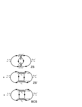
To , there are three diagrams resulting in nonzero connected contributions to the linear DC conductance, depicted in Fig. 14. The corresponding 4-point functions read
| (190a) | ||||
| (190b) |
| (190c) |
Here the terminology of BCS, ZS and ZS′ is borrowed from Ref. Shankar, 1994 and refers only to the topology of the diagrams.
We illustrate the calculation with the BCS diagram; ZS and ZS’ again turn out to be completely analogous. Going to the Fourier space,
| (191) |
the summation is standard, whereas the and summations require the following identities:
| (192a) | |||
| and | |||
| (192b) |
where . The second identity can be derived by allowing the complex plane contour to wrap around the line .Mahan (2000)
After applying the identities above, performing analytic continuation , and performing all integrals that are approachable by the contour method in Eq. (188), we find
| (193) |
In the DC limit, the principal value parts of the integrands cancel to , while the -function parts remain:
| (194) |
In the second step we have again invoked Eq. (187).
Each of the ZS and ZS’ contributions ends up being the opposite of the BCS contribution,
| (195) |
therefore, using Eq. (10) for the matrix elements, we can express the total connected contribution to the conductance to as
| (196) |
where
| (197) |
We have reintroduced the coupling matrix Eq. (8). The integral can be done explicitly:
| (198) |
i.e. the lowest order connected contribution to the conductance is , characteristic of a Fermi liquid.
Appendix E Non-interacting Schroedinger equations for the open long ring
In this appendix we sketch how to obtain Eq. (104) which expresses, in terms of incident amplitudes , the scattered amplitudes in the main leads , and the coupling site wave functions , . Because the Schroedinger equation is linear and all incident amplitudes are independent, we can let all but one of the incident amplitudes be zero at a time, and obtain the full solution by means of linear superposition.
When the incident amplitudes from the side leads are all zero , according to Eq. (97) the wave function at wave vector takes the form
| (202) |
To characterize the two Y-junctions in the AB ring, it is convenient to introduce the auxiliary objects and :
| (203) |
| (204) |
The physical meaning of and is discussed below Eq. (104). For our model we can find explicitly by solving the Schroedinger equations,
| (205a) |
| (205b) |
| (205c) |
| (205d) |
where is the wave function on the central site of the left Y-junction. We can solve for in a similar fashion.
For given and , Eq. (202) has unknowns. Now that and are known, Eqs. (203) and (204) provide us with equations. The remaining two equations are the open boundary conditions at the ends of the two QD arms, appropriate when the QD is decoupled:
| (206) |
| (207) |
It is straightforward to solve the closed set of equations.
On the other hand, when we let one of the incident amplitudes in the side leads be nonzero, there are two additional amplitudes in the wave function. For instance, if for a given , we need to effectuate the following changes to the wave function on the left QD arm in Eq. (202):
| (208) |
should be replaced by in Eq. (206) and by in Eq. (203). Furthermore, we should have two boundary conditions at site :
| (209) |
| (210) |
thus closing the set of equations. The last equation is none other than Eq. (96).
Solving all four different sets of equations in the limit of and and combining the solutions, we promptly arrive at Eq. (104).
References
- Kondo (1964) J. Kondo, Prog. Theor. Phys. 32, 37 (1964).
- Hewson (1997) A. Hewson, The Kondo Problem to Heavy Fermions, Cambridge Studies in Magnetism (Cambridge University Press, 1997).
- Anderson (1970) P. W. Anderson, J. Phys. C 3, 2436 (1970).
- Wilson (1975) K. G. Wilson, Rev. Mod. Phys. 47, 773 (1975).
- Nozières (1974) P. Nozières, J. Low Temp. Phys. 17, 31 (1974).
- Zaránd et al. (2004) G. Zaránd, L. Borda, J. von Delft, and N. Andrei, Phys. Rev. Lett. 93, 107204 (2004).
- Borda et al. (2007) L. Borda, L. Fritz, N. Andrei, and G. Zaránd, Phys. Rev. B 75, 235112 (2007).
- Micklitz et al. (2006) T. Micklitz, A. Altland, T. A. Costi, and A. Rosch, Phys. Rev. Lett. 96, 226601 (2006).
- Pierre and Birge (2002) F. Pierre and N. O. Birge, Phys. Rev. Lett. 89, 206804 (2002).
- Goldhaber-Gordon et al. (1998) D. Goldhaber-Gordon, H. Shtrikman, D. Mahalu, D. Abusch-Magder, U. Meirav, and M. A. Kastner, Nature 391, 156 (1998).
- Cronenwett et al. (1998) S. M. Cronenwett, T. H. Oosterkamp, and L. P. Kouwenhoven, Science 281, 540 (1998).
- Simmel et al. (1999) F. Simmel, R. H. Blick, J. P. Kotthaus, W. Wegscheider, and M. Bichler, Phys. Rev. Lett. 83, 804 (1999).
- van der Wiel et al. (2000) W. G. van der Wiel, S. D. Franceschi, T. Fujisawa, J. M. Elzerman, S. Tarucha, and L. P. Kouwenhoven, Science 289, 2105 (2000).
- Pustilnik and Glazman (2004) M. Pustilnik and L. Glazman, J. Phys. Condens. Matter 16, R513 (2004).
- Glazman and Pustilnik (2005) L. I. Glazman and M. Pustilnik, “Nanophysics: Coherence and transport,” (Elsevier, 2005) pp. 427–478.
- Pereira et al. (2008) R. G. Pereira, N. Laflorencie, I. Affleck, and B. I. Halperin, Phys. Rev. B 77, 125327 (2008).
- Simon and Affleck (2002) P. Simon and I. Affleck, Phys. Rev. Lett. 89, 206602 (2002).
- Simon and Affleck (2003) P. Simon and I. Affleck, Phys. Rev. B 68, 115304 (2003).
- Cornaglia and Balseiro (2003) P. S. Cornaglia and C. A. Balseiro, Phys. Rev. Lett. 90, 216801 (2003).
- Park et al. (2013) J. Park, S.-S. B. Lee, Y. Oreg, and H.-S. Sim, Phys. Rev. Lett. 110, 246603 (2013).
- Thimm et al. (1999) W. B. Thimm, J. Kroha, and J. von Delft, Phys. Rev. Lett. 82, 2143 (1999).
- Cornaglia and Balseiro (2002) P. S. Cornaglia and C. A. Balseiro, Phys. Rev. B 66, 115303 (2002).
- Kaul et al. (2005) R. K. Kaul, D. Ullmo, S. Chandrasekharan, and H. U. Baranger, Europhys. Lett. 71, 973 (2005).
- Simon et al. (2006) P. Simon, J. Salomez, and D. Feinberg, Phys. Rev. B 73, 205325 (2006).
- Kaul et al. (2006) R. K. Kaul, G. Zaránd, S. Chandrasekharan, D. Ullmo, and H. U. Baranger, Phys. Rev. Lett. 96, 176802 (2006).
- Liu et al. (2012a) D. E. Liu, S. Burdin, H. U. Baranger, and D. Ullmo, Europhys. Lett. 97, 17006 (2012a).
- Liu et al. (2012b) D. E. Liu, S. Burdin, H. U. Baranger, and D. Ullmo, Phys. Rev. B 85, 155455 (2012b).
- Simon et al. (2005) P. Simon, O. Entin-Wohlman, and A. Aharony, Phys. Rev. B 72, 245313 (2005).
- Yoshii and Eto (2011) R. Yoshii and M. Eto, Phys. Rev. B 83, 165310 (2011).
- Affleck and Simon (2001) I. Affleck and P. Simon, Phys. Rev. Lett. 86, 2854 (2001).
- Simon and Affleck (2001) P. Simon and I. Affleck, Phys. Rev. B 64, 085308 (2001).
- Komijani et al. (2013) Y. Komijani, R. Yoshii, and I. Affleck, Phys. Rev. B 88, 245104 (2013).
- Glazman and Raikh (1988) L. Glazman and M. Raikh, JETP Lett. 47, 452 (1988).
- Bruder et al. (1996) C. Bruder, R. Fazio, and H. Schoeller, Phys. Rev. Lett. 76, 114 (1996).
- Pustilnik and Glazman (2001) M. Pustilnik and L. I. Glazman, Phys. Rev. B 64, 045328 (2001).
- Malecki and Affleck (2010) J. Malecki and I. Affleck, Phys. Rev. B 82, 165426 (2010).
- Meir and Wingreen (1992) Y. Meir and N. S. Wingreen, Phys. Rev. Lett. 68, 2512 (1992).
- Jauho et al. (1994) A.-P. Jauho, N. S. Wingreen, and Y. Meir, Phys. Rev. B 50, 5528 (1994).
- Dinu et al. (2007) I. V. Dinu, M. Ţolea, and A. Aldea, Phys. Rev. B 76, 113302 (2007).
- Zaffalon et al. (2008) M. Zaffalon, A. Bid, M. Heiblum, D. Mahalu, and V. Umansky, Phys. Rev. Lett. 100, 226601 (2008).
- Schuster et al. (1997) R. Schuster, E. Buks, M. Heiblum, D. Mahalu, V. Umansky, and H. Shtrikman, Nature 385, 417 (1997).
- Ji et al. (2000) Y. Ji, M. Heiblum, D. Sprinzak, D. Mahalu, and H. Shtrikman, Science 290, 779 (2000).
- Ji et al. (2002) Y. Ji, M. Heiblum, and H. Shtrikman, Phys. Rev. Lett. 88, 076601 (2002).
- Avinun-Kalish et al. (2005) M. Avinun-Kalish, M. Heiblum, O. Zarchin, D. Mahalu, and V. Umansky, Nature 436, 529 (2005).
- Takada et al. (2014) S. Takada, C. Bäuerle, M. Yamamoto, K. Watanabe, S. Hermelin, T. Meunier, A. Alex, A. Weichselbaum, J. von Delft, A. Ludwig, A. D. Wieck, and S. Tarucha, Phys. Rev. Lett. 113, 126601 (2014).
- Carmi et al. (2012) A. Carmi, Y. Oreg, M. Berkooz, and D. Goldhaber-Gordon, Phys. Rev. B 86, 115129 (2012).
- Aharony et al. (2002) A. Aharony, O. Entin-Wohlman, B. I. Halperin, and Y. Imry, Phys. Rev. B 66, 115311 (2002).
- Aharony and Entin-Wohlman (2005) A. Aharony and O. Entin-Wohlman, Phys. Rev. B 72, 073311 (2005).
- Entin-Wohlman et al. (2005) O. Entin-Wohlman, A. Aharony, and Y. Meir, Phys. Rev. B 71, 035333 (2005).
- Kashcheyevs et al. (2006) V. Kashcheyevs, A. Aharony, and O. Entin-Wohlman, Phys. Rev. B 73, 125338 (2006).
- Schrieffer and Wolff (1966) J. R. Schrieffer and P. A. Wolff, Phys. Rev. 149, 491 (1966).
- Affleck and Ludwig (1993) I. Affleck and A. W. W. Ludwig, Phys. Rev. B 48, 7297 (1993).
- Ng and Lee (1988) T. K. Ng and P. A. Lee, Phys. Rev. Lett. 61, 1768 (1988).
- Mahan (2000) G. Mahan, Many-Particle Physics, Physics of Solids and Liquids (Springer, 2000).
- Affleck et al. (2008) I. Affleck, L. Borda, and H. Saleur, Phys. Rev. B 77, 180404 (2008).
- Miroshnichenko et al. (2010) A. E. Miroshnichenko, S. Flach, and Y. S. Kivshar, Rev. Mod. Phys. 82, 2257 (2010).
- Vojta and Fritz (2004) M. Vojta and L. Fritz, Phys. Rev. B 70, 094502 (2004).
- Fritz and Vojta (2004) L. Fritz and M. Vojta, Phys. Rev. B 70, 214427 (2004).
- Gerland et al. (2000) U. Gerland, J. von Delft, T. A. Costi, and Y. Oreg, Phys. Rev. Lett. 84, 3710 (2000).
- Hofstetter et al. (2001) W. Hofstetter, J. König, and H. Schoeller, Phys. Rev. Lett. 87, 156803 (2001).
- Silvestrov and Imry (2003) P. G. Silvestrov and Y. Imry, Phys. Rev. Lett. 90, 106602 (2003).
- Oreg and Goldhaber-Gordon (2003) Y. Oreg and D. Goldhaber-Gordon, Phys. Rev. Lett. 90, 136602 (2003).
- Potok et al. (2007) R. M. Potok, I. G. Rau, H. Shtrikman, Y. Oreg, and D. Goldhaber-Gordon, Nature 446, 167 (2007).
- Bellazzini et al. (2007) B. Bellazzini, M. Mintchev, and P. Sorba, J. Phys. A 40, 2485 (2007).
- Perelomov et al. (1998) A. Perelomov, Â. Zel’dovič, and I. Zelʹdovich, Quantum Mechanics: Selected Topics, Selected Topics Series (World Scientific, 1998).
- Shankar (1994) R. Shankar, Rev. Mod. Phys. 66, 129 (1994).