Duality and Conditional Expectations in the Nakajima-Mori-Zwanzig Formulation

Abstract

We develop a new operator algebraic formulation of the Nakajima-Mori-Zwanzig (NMZ) method of projections. The new theory is built upon rigorous mathematical foundations, and it can be applied to both classical and quantum systems. We show that a duality principle between the NMZ formulation in the space of observables and in the state space can be established, analogous to the Heisenberg and Schrödinger pictures in quantum mechanics. Based on this duality we prove that, under natural assumptions, the projection operators appearing in the NMZ equation must be conditional expectations. The proposed formulation is illustrated in various examples.

I Introduction

High-dimensional stochastic dynamical systems arise in many areas of mathematics, natural sciences and engineering. Whether it is a physical system being studied in a lab, or an equation being solved on a computer, the full microscopic state of the system as a point evolving in some phase space is often intractable to handle in all its complexity.

Instead, it is often desirable to attempt to reduce the complexity of the theoretical description by passing from a model of the dynamics of the full system to a model only of the observables of interest. Such observables may be chosen, for example, because they represent global macroscopic features of the bulk system, as in the derivation of the Boltzmann equation of nonequilibrium thermodynamics from microscopic descriptions Villani (2002); Snook (2006); Cercignani, Gerasimenko, and Petrina (2012), or in the derivation of the dynamics of commutative subalgebras of observables in quantum mechanics Kolomietz and Radionov (2010). The observables may also represent features localized on a subsystem of interest, as in the Brownian motion of a particle in a liquid, where the master equation governing the position and momentum of the particle is derived from first principles (Hamiltonian equations of motion of the full system), by eliminating the degrees of freedom associated with the surrounding liquid van Kampen and Oppenheim (1986); Chaturvedi and Shibata (1979). In the context of numerical approximation of stochastic partial differential equations (SPDEs), the observables may be chosen to define a finite-dimensional approximation of the phase space, for example a finite set of Fourier-Galerkin coefficients Edwards (1964); Herring (1966); Montgomery (1976). Whatever the reason behind this reduction of the set of observables, it is often desirable to then attempt to reduce the complexity of the theoretical description by passing from a model of the dynamics of the full system to a model only of the observables of interest. For example, we might have a high-dimensional dynamical system evolving as $dx/dt=F(x)$, but we are only interested in a relatively small number of $\mathbb{C}$-valued observable functions $g_{1}(x),\dots,g_{m}(x)$. The dynamics of this lower-dimensional set of observable quantities may be simpler than that of the entire system, although the underlying law by which such quantities evolve in time is often quite complex. Nevertheless, approximation of such law can in many cases allow us to avoid performing simulation of the full system and solve directly for the quantities of interest. If the resulting equation for $\{g_{i}(x)\}$ is low dimensional and computable, this provides a means of avoiding the curse of dimensionality.

In this paper we study one family of techniques for performing such dimensional reduction, namely the Nakajima-Mori-Zwanzig (NMZ) method of projections Nakajima (1958); Mori (1965); Zwanzig (1960, 1961) (see also Chorin, Hald, and Kupferman (2000); Venturi, Cho, and Karniadakis (2016); Venturi and Karniadakis (2014)). To this end, we place the NMZ formulation in the context of $C^{*}$-algebras of observables, and in so doing, set rigorous foundations of this important and widely used technique. More importantly, the operator algebraic setting we propose unifies classical and quantum mechanical formulations. The method of projections derives its name from the use of a projection map from the algebra of observables of the full system, to the subalgebra of interest. In this algebraic context, it will naturally emerge that the two common flavors of NMZ – for “phase space functions” and for probability density functions (PDFs) – are dual equations for observables and states, directly corresponding to the dual Schrödinger and Heisenberg pictures of quantum mechanics. Reasoning about information in these algebras and desiderata of the NMZ projection will reveal that the projection must be a conditional expectation in the operator algebraic sense.

The paper is organized as follows. We begin in Section II with a quick review of $C^{*}$-algebras, their states and homomorphisms, as well as the relationship between topological spaces and algebras of functions. We then discuss the relationship between classical dynamical systems and observable algebras in Section III, deriving from the nonlinear dynamical system the equivalent linear dynamics on the observable algebra. In Section IV, the NMZ equation is introduced for the reduced dynamics on an observable algebra, along with the dual NMZ equation on the states of the algebra. We then look more closely at the NMZ projection operator in Section V, finding that, under natural assumptions, the projection operator must be a conditional expectation. While the elements of $C^{*}$-algebras are bounded observables, it is common to consider also unbounded observables (such as momentum); the incorporation of such affiliated observables into the NMZ framework is considered in Section V.2. In Section VI, we consider the problem of “pushing” the dynamics from one space to another (typically lower dimensional) space using NMZ and discuss the application of NMZ to quantum open systems. In Section VII two simple examples of the NMZ method are carried out analytically. Finally, the main results are summarized in Section VIII. We also include two brief Appendices, in which we discuss technical questions related to non-degenerate homeomorphisms and state-preserving maps.

II Background

In this section we provide a quick review of $C^{*}$-algebras, their states and homomorphisms, and relationship between topological spaces and algebras of functions. The material in this section is well-known and can be found throughout the literature on operator algebras and algebraic dynamics. Standard references for much of this material include, e.g., Kadison and Ringrose (1997); Takesaki (2002); Bratteli and Robinson (2003); Blackadar (2006).

II.1 $C^{*}$-Algebras of Observables

We are interested in developing the NMZ formalism simultaneously for dynamical systems

$$\dot{x}=F(x,\xi,t)$$ (1)

evolving on a (sufficiently) smooth manifold $\mathcal{M}$, where $\xi$ represents parameters drawn (perhaps randomly) from some parameter space $\Xi$, as well as for quantum mechanical systems. By “manifold” here we mean any of a large class of spaces on which (1) makes sense, including, at a minimum, finite-dimensional manifolds, Banach spaces, and more general Banach manifolds. In particular, the simple form of (1) can represent many different kinds of initial value problem, including ODEs, PDEs, and functional differential equations Venturi (2016). Thinking first of the classical dynamical system above, and of $\mathcal{M}$ as a generalized phase space of the system, a classical observable will typically be a $\mathbb{C}$-valued function on $\mathcal{M}$. There are different possible choices for the set of such functions, but certain properties may be desirable Segal (1947); Strocchi (2008). For example, if we can observe $f$ and $g$, then we should be able to observe $\alpha f+\beta g$ for any $\alpha,\beta\in\mathbb{C}$. We should also expect to be able to observe the product $fg$. In this way, we should expect the space of observables to form an algebra of functions under pointwise addition and multiplication. More careful and detailed reasoning Strocchi (2008) about arbitrary physical systems (be they classical or quantum) leads to the conclusion that the set of observables for any physical system can be represented as a $C^{*}$-algebra. That algebra will generally be commutative in the classical case, and noncommutative in the quantum case.

A Banach algebra is an algebra $\mathfrak{A}$ over $\mathbb{C}$ with a norm making $\mathfrak{A}$ a Banach space, and such that $\|xy\|\leq\|x\|\|y\|$ for all $x,y\in\mathfrak{A}$. A $C^{*}$-algebra is a Banach algebra $\mathfrak{A}$ with an isometric involution $x\mapsto x^{*}$ such that $(xy)^{*}=y^{*}x^{*}$ for all $x,y\in\mathfrak{A}$, and such that $\|x^{*}x\|=\|x\|^{2}$ for all $x\in\mathfrak{A}$.

An important subclass of $C^{*}$-algebras is formed by the von Neumann (i.e. $W^{*}$-) algebras, which are unital $C^{*}$-algebras closed with respect to the ultraweak topology. They can be characterized as those $C^{*}$-algebras which admit a Banach space predual Sakai (1956), i.e. a Banach space whose dual space is (isomorphic to) the $C^{*}$-algebra. Two key commutative algebras of functions to keep in mind are

1. $\mathfrak{A}=C_{0}(\mathcal{M})$. This is the algebra of continuous $\mathbb{C}$-valued functions on $\mathcal{M}$ “vanishing at infinity”. This means that for any $f\in\mathfrak{A}$ and any $\epsilon>0$, the set $\{x\in\mathcal{M}\;:\;|f(x)|\geq\epsilon\}$ is compact within $\mathcal{M}$. The algebra $C_{0}(\mathcal{M})$ is endowed with the $\sup$ norm, i.e. $\|f\|=\sup_{x\in\mathcal{M}}\|f(x)\|$. It is a unital algebra if and only if $\mathcal{M}$ is compact, in which case the identity is the function that is everywhere equal to one: $\mathds{1}(x)=1$ for all $x\in\mathcal{M}$. The dual space ${\mathfrak{A}^{\ast}}$ is isometrically isomorphic to the space $\mathfrak{M}(\mathcal{M})$ of all complex-valued regular Borel measures (i.e. Radon measures) with finite norm

   $$\|\nu\|=\sup_{f\in C_{0}(\mathcal{M})}\frac{\left|\int_{\mathcal{M}}f(x)\,{d}\nu(x)\right|}{\|f\|}.$$ (2)

2. $\mathfrak{A}=L^{\infty}(\mathcal{M},\mu)$. This is the algebra of (equivalence classes of) essentially bounded $\mathbb{C}$-valued measurable functions on $\mathcal{M}$, for some choice of localizable Segal (1951) regular Borel measure (i.e. Radon measure) $\mu$ on $\mathcal{M}$. The norm on this algebra is the essential supremum $\|f\|=\inf\{r>0\;:\;|f(x)|\leq r\quad\mu\text{-a.e.}\}$. The dual space ${\mathfrak{A}^{\ast}}$ is isometrically isomorphic to the space of finitely additive localizable complex-valued Borel measures absolutely continuous with respect to $\mu$ and with finite norm

   $$\|\nu\|=\sup_{f\in L^{\infty}(\mathcal{M},\mu)}\frac{\left|\int_{\mathcal{M}}f(x)\,{d}\nu(x)\right|}{\|f\|}.$$ (3)

   $L^{\infty}(\mathcal{M},\mu)$ is a von Neumann algebra, and, as such, admits a unique (up to isometric isomorphism) predual ${{L^{\infty}(\mathcal{M},\mu)}_{\ast}}$, which can be identified with $L^{1}(\mathcal{M},\mu)$. Of course, $L^{1}(\mathcal{M},\mu)$ can itself be identified with the space of localizable $\mathbb{C}$-valued Borel measures absolutely continuous with respect to $\mu$.

II.2 Order Structure and States

A function $g$ in $\mathfrak{A}=C_{0}(\mathcal{M})$ or $\mathfrak{A}=L^{\infty}(\mathcal{M},\mu)$ is considered to be positive if $g(x)\geq 0$ everywhere (or almost everywhere, as appropriate). This will be denoted $g\geq 0$. More abstractly, in a general $C^{*}$-algebra $\mathfrak{A}$, $G\geq 0$ if there exist $H\in\mathfrak{A}$ such that $G=H^{*}H$. The positive elements of $\mathfrak{A}$ form a closed convex cone. An element $\phi$ of the Banach dual space ${\mathfrak{A}^{\ast}}$ is positive if $\phi(G)\geq 0$ for all $G\geq 0$. And $\phi\in{\mathfrak{A}^{\ast}}$ is a state if it is positive and $\|\phi\|=1$. Note that, in the case that $\mathfrak{A}$ is unital, the normalization condition $\|\phi\|=1$ is equivalent to $\phi(\mathds{1})=1$. We will denote the set of states as $\mathcal{S}(\mathfrak{A})\subset{\mathfrak{A}^{\ast}}$. The equivalence of ${\mathfrak{A}^{\ast}}$ with a Banach space of $\mathbb{C}$-valued (at least finitely additive) measures on $\mathcal{M}$ implies that $\mathcal{S}(\mathfrak{A})$ can be identified with the subset of probability measures on $\mathcal{M}$. Thus for any $\rho\in\mathcal{S}(\mathfrak{A})$ and any $G\in\mathfrak{A}$, $\rho(G)$ is the expectation value of $G$ over the state (probability measure) $\rho$. In other words, if $\hat{\rho}$ is the measure associated with the state $\rho$, then $\rho(G)$ can be interpreted as

$$\rho(G)=\int_{\mathcal{M}}G(x)\,{d}\hat{\rho}(x).$$

When $\mathfrak{A}$ is a von Neumann algebra such as $L^{\infty}(\mathcal{M},\mu)$, we identify the positive cone in the predual ${{\mathfrak{A}}_{\ast}}$ as follows: for any $\phi\in{{\mathfrak{A}}_{\ast}}$, $\phi\geq 0$ if $G(\phi)\geq 0$ for all $G\geq 0$ in $\mathfrak{A}$. The set of normal states $\mathcal{S}_{N}(\mathfrak{A})$ is the set of $\rho\in{{\mathfrak{A}}_{\ast}}$ such that $\rho\geq 0$ and $\|\rho\|=1$. Because of the added complications that finitely additive measures impose, it may be advantageous to work with states in the predual when we take $\mathfrak{A}=L^{\infty}(\mathcal{M},\mu)$. In what follows, we will use the notation associated with duals (rather than preduals), but replacing this with the predual (and normal states) in the case of von Neumann algebras is straightforward.

Although $\rho(G)$ is the expectation value of $G$, the state $\rho$ carries more detailed statistical information about the result of measuring the observable $G$. Indeed, repeated measurements of a normal observable $G$ (meaning $G^{*}G=GG^{*}$) against an ensemble of systems in identical states does not simply yield the expectation value, but samples from a probability measure of values. Let $\mathfrak{A}$ be any unital $C^{*}$-algebra and $\rho\in\mathcal{S}(A)$ be a state; if $\mathfrak{A}$ is not unital, pass to the unitization $\tilde{\mathfrak{A}}$ and extend $\rho$ by $\rho(\mathds{1})=1$ to a state of $\tilde{\mathfrak{A}}$. For any normal $G\in\mathfrak{A}$, let $\sigma(G)\subset\mathbb{C}$ (topologized as a compact subset of $\mathbb{C}$) be the spectrum of $G$, and $C(\sigma(G))$ the $C^{*}$-algebra of continuous $\mathbb{C}$-valued functions on $\sigma(G)$. There is a continuous functional calculus, expressible as a unital $*$-morphism $\Phi_{G}:C(\sigma(G))\to\mathfrak{A}$, which is an isomorphism onto the unital subalgebra of $\mathfrak{A}$ generated by $G$ [Takesaki, 2002, Prop. I.4.6]. Then $\rho_{G}:=\Phi_{G}^{*}\rho$ is a state of $C(\sigma(G))$, and therefore may be identified through the Riesz-Markov theorem with a Radon probability measure on $\sigma(G)$, or equivalently with a Radon probability measure $\mu$ on $\mathbb{C}$ that is supported on $\sigma(G)$. This measure describes the probability of observing value $\lambda\in\mathbb{C}$ when measuring observable $G$ on a system in state $\rho$.

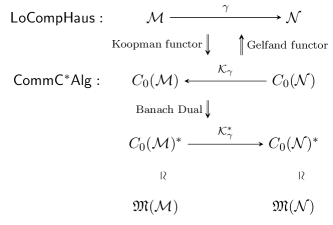
Figure 1: Sketch of typical spaces and maps associated with the Gelfand representation of locally compact Hausdorff spaces and proper maps.

II.3 Categories of Interest

Here we briefly review some categories of topological spaces, measure spaces, and algebras that will be relevant to the remainder of the paper.

• LoCompHaus: locally compact Hausdorff topological spaces with proper continuous maps.

• CommC^∗Alg: commutative (not necessarily unital) $C^{*}$ algebras with continuous (i.e. bounded) non-degenerate ^∗-homomorphisms. Here $f:\mathfrak{A}\to\mathfrak{B}$ non-degenerate means $\operatorname{Span}_{\mathbb{C}}\{f(a)b\;:\;a\in\mathfrak{A},b\in\mathfrak{B}\}$ is dense in $\mathfrak{B}$ Brandenburg (2007). See also Lemma 1 in Appendix A for an alternative characterization of non-degenerate morphisms.

• LocMeas: Localizable measure spaces Segal (1951) with non-singular measurable functions (defined almost everywhere), i.e. $f:(X,\Sigma,\mu)\to(Y,\Sigma^{\prime},\nu)$ is such that $\mu(f^{-1}(A))=0$ whenever $\nu(A)=0$.

• CommVNA: commutative (unital) von Neumann algebras with ultraweakly continuous unital ^∗-homomorphisms.

• C^∗Alg: (not necessarily unital) $C^{*}$ algebras with continuous (i.e. bounded) non-degenerate ^∗-homomorphisms.

• vNAlg: (unital) von Neumann algebras with ultraweakly continuous unital ^∗-homomorphisms.

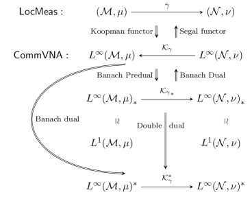
Figure 2: Sketch of typical spaces and maps associated with the Segal representation of localizable measure spaces and measurable maps.

When describing the NMZ formalism for a dynamical system evolving on a manifold (perhaps infinite-dimensional), we will be working largely in the two categories of commutative algebras CommC^∗Alg and CommVNA. The more general setting – including the NMZ formalism for quantum mechanics – involves the categories of noncommutative algebras C^∗Alg and vNAlg.

Gelfand duality Bratteli and Robinson (2003); Brandenburg (2007) implies that LoCompHaus is equivalent to CommC^∗Alg^op (see Figure 1). Thus, for example, any commutative $C^{*}$ algebra is realizable as the algebra $C_{0}(X)$ of continuous functions vanishing at infinity on an essentially unique locally compact Hausdorff (LCH) topological space $X$, and every nondegenerate $C^{*}$-homomorphism between such algebras is realizable as an essentially unique proper map between LCH spaces. A similar Segal duality Segal (1951) implies that LocMeas is equivalent to CommVNA^op (see Figure 2). These duality theories, which we discuss further in the next subsection, allow for the transformation from nonlinear dynamical systems to completely equivalent linear dynamical systems in Banach spaces.

II.4 Composition and Transfer Operators

We will make extensive use of the composition operator (i.e., the Koopman operator Koopman (1931)) and its adjoint, the transfer operator (i.e., the Perron-Frobenius operator) Beck and Schlögl (1995); Sarig (2012). Let $\gamma:\mathcal{M}\to\mathcal{N}$ be a continuous map. In keeping with our definitions of LoCompHaus and LocMeas, we require that $\gamma$ is non-singular: in LoCompHaus we require that $\gamma$ is proper (the pre-image of a compact set is compact), and in LocMeas we require that $\mu(\gamma^{-1}(A))=0$ whenever $\nu(A)=0$ (where $\nu$ is the Borel measure on $\mathcal{N}$). Then the composition operator (Koopman) $\mathcal{K}_{\gamma}$ is the $C^{*}$-homomorphism from $\mathfrak{B}=C_{0}(\mathcal{N})$ to $\mathfrak{A}=C_{0}(\mathcal{M})$ (or from $\mathfrak{B}=L^{\infty}(\mathcal{N},\nu)$ to $\mathfrak{A}=L^{\infty}(\mathcal{M},\mu)$), defined by

$$\mathcal{K}_{\gamma}g=g\circ\gamma.$$ (4)

As it is a $C^{*}$-homomorphism, $\mathcal{K}_{\gamma}$ is contractive, i.e., $\|\mathcal{K}_{\gamma}\|\leq 1$. In fact, it is easy to see that $\|\mathcal{K}_{\gamma}\|=1$, since one can construct a nontrivial $g\in\mathfrak{B}$ supported in the range of $\gamma$, for which we clearly have $\|\mathcal{K}_{\gamma}g\|=\|g\|$ (see Lemma 3 in Appendix A).

The dual of the composition operator is the transfer operator (Perron Frobenius)Lasota and Mackey (2008) ${\mathcal{K}_{\gamma}^{\ast}}:{\mathfrak{A}^{\ast}}\to{\mathfrak{B}^{\ast}}$ which essentially “pushes” states forward along $\gamma$. It is straightforward to show that ${\mathcal{K}_{\gamma}^{\ast}}$ is positive and contractive, i.e. $\|{\mathcal{K}_{\gamma}^{\ast}}\phi\|\leq\|\phi\|$ for all $\phi\in{\mathfrak{A}^{\ast}}$. Moreover, for any $\phi\geq 0$ in ${\mathfrak{A}^{\ast}}$, $\|{\mathcal{K}_{\gamma}^{\ast}}\phi\|=\|\phi\|$ (see Lemma 4 in Appendix A), so that ${\mathcal{K}_{\gamma}^{\ast}}\mathcal{S}(\mathfrak{A})\subset\mathcal{S}(\mathfrak{B})$. When $\mathfrak{A}=C_{0}(\mathcal{M})$ and $\mathfrak{B}=C_{0}(\mathcal{N})$, then ${\mathfrak{A}^{\ast}}\simeq\mathfrak{M}(\mathcal{M})$ (the space of Radon measures on $\mathcal{M}$), ${\mathcal{B}^{\ast}}\simeq\mathfrak{M}(\mathcal{N})$, and for any measurable $B\subset\mathcal{N}$ and $\mu\in\mathfrak{M}(\mathcal{M})$, $({\mathcal{K}_{\gamma}^{\ast}}\mu)(B)=\mu(\gamma^{-1}(B))$. In the von Neumann algebra setting, when ${{\mathfrak{A}}_{\ast}}\simeq L^{1}(\mathcal{M},\mu)$ and ${{\mathfrak{B}}_{\ast}}\simeq L^{1}(\mathcal{N},\nu)$, the transfer operator ${{\mathcal{K}_{\gamma}}_{\ast}}$ may be regarded as a transformation between $L^{1}$ functions, defined via the Radon-Nikodym derivative

$$\big{(}{{\mathcal{K}_{\gamma}}_{\ast}}\rho\big{)}(y)=\frac{{d}\eta_{\rho}}{{d}\nu}(y)$$ (5)

for all $y\in\mathcal{N}$, where $\eta_{\rho}$ is the push-forward measure on $\mathcal{N}$ given by

$$\eta_{\rho}(A):=\int_{\gamma^{-1}(A)}\rho(x){d}\mu(x).$$

II.5 Partial Information

Given the $C^{*}$-algebra of observables $\mathfrak{A}$ on our system, we may choose to only observe the system through a subcollection $C\subset\mathfrak{A}$. By only viewing the system through these observables in $C$, we obtain only partial information (relative to that obtained from using all of the observables in $\mathfrak{A}$). However, the set $C$ may not fully represent the set of observables whose value we know if we observe using $C$. For example, if $f,g\in C$, then we know the value of $\alpha f+\beta g\in\mathfrak{A}$ for any $a,b\in\mathbb{C}$. We also know the value of $f^{*}$, $g^{*}$, and, at least when $f$ and $g$ commute, we know the value of $fg$. So, to represent the set of observables whose value we know after measurement, we must expand any mutually commuting set of observables $C$ at least to the $*$-algebra containing $C$. In this paper (and in keeping with much of the literature in quantum mechanics and quantum information) we generally view partial information only through the lens of $C^{*}$-subalgebras of observables.

III Nonlinear Dynamical Systems

Consider a nonautonomous dynamical system in the form (1) and assume that the flow $\Phi(t,t_{0})$ exists for all $t\geq t_{0}$. Let $\mathfrak{A}$ be a commutative $C^{*}$-algebra of $\mathbb{C}$-valued “observable” functions on a manifold $\mathcal{M}$, and let $\mathcal{K}_{\Phi(t,s)}$ be the Koopman operator associated with $\Phi(t,s)$. Clearly, $\mathcal{K}_{\Phi(t,s)}$ is a $*$-endomorphism acting on $\mathfrak{A}$.

III.1 Composition and Transfer Operators

Let $\Phi(t,t_{0})$ be the flow generated by the dynamical system (1). For any observable $g(x)$ we have

$$g(x(t))=\mathcal{K}_{\Phi(t,t_{0})}g(x_{0}).$$ (6)

By differentiating this equation with respect to $t$ we obtain

$$\frac{{d}}{{d}t}\mathcal{K}_{\Phi(t,t_{0})}g(x_{0}) =\mathcal{K}_{\Phi(t,t_{0})}\mathcal{L}_{F^{\xi}_{t}}g(x_{0}),$$ (7)

where $F_{t}^{\xi}=F(\cdot,\xi,t)$ is the vector field from (1) at fixed $t$ and $\xi$, and $\mathcal{L}_{F^{\xi}_{t}}g={d}g(F_{t}^{\xi})$ is an ultraweakly densely defined, ultraweakly closed, generally unbounded linear operator on $\mathfrak{A}$. Therefore,

$$\frac{{d}}{{d}t}\mathcal{K}_{\Phi(t,t_{0})} =\mathcal{K}_{\Phi(t,t_{0})}\mathcal{L}_{F^{\xi}_{t}},$$ (8)

which implies

$$\mathcal{K}_{\Phi(t,s)} =\operatorname{\overrightarrow{\mathcal{T}}}e^{\int_{s}^{t}\mathcal{L}_{F^{\xi}_{\tau}}\,{d}\tau}.$$ (9)

Here $\operatorname{\overrightarrow{\mathcal{T}}}$ is the time-ordering operator placing later operators to the right. It should be noted that, for time-dependent $\mathcal{L}_{t}$ and irreversible flow $\Phi(t,t_{0})$, the observable $g(t)=g(x(t))$ doesn’t generally obey a simple evolution equation of the form ${d}g(t)/{d}t=R_{t}g(t)$. This is because there need not exist a time-dependent operator $R_{t}$ such that

$$\frac{{d}}{{d}t}g(t)=\mathcal{K}_{\Phi(t,0)}\mathcal{L}_{t}g_{0}=R_{t}\mathcal{K}_{\Phi(t,0)}g_{0}=R_{t}g(t).$$ (10)

Now, consider a fixed state $\rho_{0}\in\mathcal{S}(\mathfrak{A})$. By using (6) and (9) we have

$$\rho_{0}(g(t))=\rho_{0}\left(\operatorname{\overrightarrow{\mathcal{T}}}e^{\int_{0}^{t}\mathcal{L}_{F^{\xi}_{\tau}}\,{d}\tau}g_{0}\right).$$

Differentiation with respect to $t$ yields

$$\frac{{d}}{{d}t}\big{[}\rho_{0}(g(t))\big{]} =\rho_{0}\left(\frac{{d}}{{d}t}g(t)\right)$$

$$=\rho_{0}\left(\operatorname{\overrightarrow{\mathcal{T}}}e^{\int_{0}^{t}\mathcal{L}_{F^{\xi}_{\tau}}\,{d}\tau}\mathcal{L}_{F^{\xi}_{t}}g_{0}\right)$$

$$=\left({\mathcal{L}_{F^{\xi}_{t}}^{\ast}}\operatorname{\overleftarrow{\mathcal{T}}}e^{\int_{0}^{t}{\mathcal{L}_{F^{\xi}_{\tau}}^{\ast}}\,{d}\tau}\rho_{0}\right)(g_{0})$$

$$=\left({\mathcal{L}_{F^{\xi}_{t}}^{\ast}}\rho(t)\right)(g_{0}),$$ (11)

i.e.,

$$\frac{{d}}{{d}t}\rho(t) ={\mathcal{L}_{F^{\xi}_{t}}^{\ast}}\rho(t).$$ (12)

The formal solution to (12) is

$$\rho(t)={\mathcal{K}_{\Phi(t,s)}^{\ast}}\rho(0),$$ (13)

where

$${\mathcal{K}_{\Phi(t,s)}^{\ast}}=\operatorname{\overleftarrow{\mathcal{T}}}e^{\int_{0}^{t}{\mathcal{L}_{F^{\xi}_{\tau}}^{\ast}}\,{d}\tau}$$ (14)

is the transfer operator (Perron-Frobenius) associated to the flow map $\Phi(t,s)$. The Gelfand and Segal dualities (see Fig. 1 and Fig. 2) imply that the linear dynamics of the composition operator in $\mathcal{B}(\mathfrak{A})$ [or the linear dynamics of the transfer operator in $\mathcal{B}({\mathfrak{A}^{\ast}})$] is completely equivalent to the nonlinear dynamics generated by (1) on $\mathcal{M}$.

IV Operator Algebraic Formulation

So far we have framed the discussion around dynamical systems evolving on manifolds, leading to commutative observable algebras $\mathfrak{A}$. However, very little of what we will do will depend on the commutativity of $\mathfrak{A}$. By and large, if we have any $C^{*}$-algebra $\mathfrak{A}$ and a linear evolution operator which is an $*$-endomorphism on $\mathfrak{A}$ that evolves as in (8), it is possible to apply the NMZ formulation to obtain a generalized Langevin equation for the reduced dynamics. In particular, this applies to quantum mechanics. In this section we develop the formalism in this more general perspective.

Let $\mathfrak{A}$ be a (not necessarily commutative) $C^{*}$-algebra. We will typically let ${\mathfrak{A}^{\ast}}$ denote the Banach space dual, and $\mathcal{S}(\mathfrak{A})\subset{\mathfrak{A}^{\ast}}$, the closed convex set of positive norm one linear functionals on $\mathfrak{A}$, be the set of states on $\mathfrak{A}$. However, when $\mathfrak{A}$ is a von Neumann algebra (i.e. it admits a Banach predual), we will abuse the notation to let ${\mathfrak{A}^{\ast}}$ denote the Banach space predual, and $\mathcal{S}(\mathfrak{A})\subset{\mathfrak{A}^{\ast}}$, the closed convex set of positive norm one elements of the predual, be the set of (normal) states on $\mathfrak{A}$. A (not necessarily bounded) linear operator $\mathcal{L}$ acting on $\mathcal{A}$ is called a $\ast$-derivation if for any $f,g\in\mathfrak{A}$, $\mathcal{L}(fg^{\ast})=(\mathcal{L}f)g^{\ast}+f(\mathcal{L}g)^{\ast}$.

Suppose that we have available a time-dependent family of closed, densely defined linear $\ast$-derivations $\{\mathcal{L}_{t}\}_{0\leq t\leq T}$, along with a $*$-endomorphism $\mathcal{E}(t,s)$ on $\mathfrak{A}$, strongly continuous in both $s$ and $t$, and satisfying for $t\geq s$

$$\mathcal{E}(t,s)=\operatorname{id}_{\mathfrak{A}}+\int_{s}^{t}\mathcal{E}(\tau,s)\mathcal{L}_{\tau}\,{d}\tau,$$ (15)

i.e., satisfying, in the sense of Carathéodory, the differential equation

$$\frac{{d}}{{d}t}\mathcal{E}(t,s)=\mathcal{E}(t,s)\mathcal{L}_{t}$$ (16)

such that $\mathcal{E}(s,s)$ is the identity morphism $\operatorname{id}_{\mathfrak{A}}$ on $\mathfrak{A}$. In the case of von Neumann algebras it suffices for $\{\mathcal{L}_{t}\}$ to be weak-*-densely defined and for $\mathcal{E}(t,s)$ to be weak-* continuous in $s$ and $t$. Then

$$\mathcal{E}(t,s)=\operatorname{\overrightarrow{\mathcal{T}}}e^{\int_{s}^{t}\mathcal{L}_{\tau}\,{d}\tau}$$ (17)

is contractive, i.e., $\|\mathcal{E}(t,s)X\|\leq\|X\|$ for all $t\geq s$ and all $X\in\mathfrak{A}$, by virtue of being a $*$-endomorphism. This $\mathcal{E}(t,t_{0})$ serves as the evolution operator for observables in $\mathfrak{A}$, i.e., $\mathcal{E}(t,t_{0})(G_{0})=G(t)$. In the classical case described in Section III, $\mathcal{E}(t,t_{0})=\mathcal{K}_{\Phi(t,t_{0})}$.

IV.1 Nakajima-Mori-Zwanzig Method of Projections

We now introduce a projection $\mathcal{P}$ on $\mathfrak{A}$ and develop from it the equations that comprise the NMZ formalism. The nature and properties of $\mathcal{P}$ will be discussed in detail in section V, but for now it will suffice to assume only that $\mathcal{P}$ is a bounded linear operator acting on $\mathfrak{A}$, and that $\mathcal{P}^{2}=\mathcal{P}$. The NMZ formalism describes the evolution of observables initially in the image of the $\mathcal{P}$. Because the evolution of observables is governed by $\mathcal{E}(t,t_{0})$ (see equation (17)), we seek an evolution equation for $\mathcal{E}(t,t_{0})\mathcal{P}$. To this end, recall first the well-known Dyson identity: if

$$Y(t,s)=\operatorname{\overrightarrow{\mathcal{T}}}e^{\int_{s}^{t}A(\tau)\,{d}\tau}\quad\textrm{and}\quad Z(t,s)=\operatorname{\overrightarrow{\mathcal{T}}}e^{\int_{s}^{t}B(\tau)\,{d}\tau}$$ (18)

then

$$Y(t,t_{0})-Z(t,t_{0}) =\int_{t_{0}}^{t}\frac{d}{ds}\Big{(}Y(s,t_{0})Z(t,s)\Big{)}\,{d}s$$

$$=\int_{t_{0}}^{t}Y(s,t_{0})(A(s)-B(s))Z(t,s)\,{d}s.$$ (19)

Applying this to $Y(t,t_{0})=\mathcal{E}(t,t_{0})$ (equation (17)) and $Z(t,t_{0})=\operatorname{\overrightarrow{\mathcal{T}}}e^{\int_{t_{0}}^{t}\mathcal{Q}\mathcal{L}_{\tau}\,{d}\tau}$ (here $\mathcal{Q}=1-\mathcal{P}$ denotes the complementary projection), we find

$$\mathcal{E}(t,t_{0}) =\operatorname{\overrightarrow{\mathcal{T}}}e^{\int_{t_{0}}^{t}\mathcal{Q}\mathcal{L}_{\tau}\,{d}\tau}+\int_{t_{0}}^{t}\mathcal{E}(s,t_{0})\mathcal{P}\mathcal{L}_{s}\operatorname{\overrightarrow{\mathcal{T}}}e^{\int_{s}^{t}\mathcal{Q}\mathcal{L}_{\tau}\,{d}\tau}\,{d}s.$$ (20)

A differentiation with respect to time and composition with $\mathcal{P}$ yields the following generalized Langevin equation for $\mathcal{E}(t,t_{0})\mathcal{P}$

$$\frac{{d}}{{d}t}\mathcal{E}(t,t_{0})\mathcal{P} =\mathcal{E}(t,t_{0})\mathcal{P}\mathcal{L}_{t}\mathcal{P}+\operatorname{\overrightarrow{\mathcal{T}}}e^{\int_{t_{0}}^{t}\mathcal{Q}\mathcal{L}_{\tau}\,{d}\tau}\mathcal{Q}\mathcal{L}_{t}\mathcal{P}$$

$$\quad+\int_{t_{0}}^{t}\mathcal{E}(s,t_{0})\mathcal{P}\mathcal{L}_{s}\operatorname{\overrightarrow{\mathcal{T}}}e^{\int_{s}^{t}\mathcal{Q}\mathcal{L}_{\tau}\,{d}\tau}\mathcal{Q}\mathcal{L}_{t}\mathcal{P}\,{d}s.$$ (21)

Letting $f_{0}=\mathcal{P}g_{0}$ represent an observable initially in the image of $\mathcal{P}$, the NMZ equation describes its evolution as

$$\frac{{d}}{{d}t}f(t) =\mathcal{E}(t,t_{0})\mathcal{P}\mathcal{L}_{t}f_{0}+\operatorname{\overrightarrow{\mathcal{T}}}e^{\int_{t_{0}}^{t}\mathcal{Q}\mathcal{L}_{\tau}\,{d}\tau}\mathcal{Q}\mathcal{L}_{t}f_{0}$$

$$\quad+\int_{t_{0}}^{t}\mathcal{E}(s,t_{0})\mathcal{P}\mathcal{L}_{s}\operatorname{\overrightarrow{\mathcal{T}}}e^{\int_{s}^{t}\mathcal{Q}\mathcal{L}_{\tau}\,{d}\tau}\mathcal{Q}\mathcal{L}_{t}f_{0}\,{d}s.$$ (22)

The Banach dual of (21) yields the NMZ equation for states

$$\frac{{d}}{{d}t}{\mathcal{P}^{\ast}} {\mathcal{E}(t,t_{0})^{\ast}}={\mathcal{P}^{\ast}}{\mathcal{L}_{t}^{\ast}}{\mathcal{P}^{\ast}}{\mathcal{E}(t,t_{0})^{\ast}}+{\mathcal{P}^{\ast}}{\mathcal{L}_{t}^{\ast}}\operatorname{\overleftarrow{\mathcal{T}}}e^{\int_{t_{0}}^{t}{\mathcal{Q}^{\ast}}{\mathcal{L}_{\tau}^{\ast}}\,{d}\tau}{\mathcal{Q}^{\ast}}$$

$$+{\mathcal{P}^{\ast}}{\mathcal{L}_{t}^{\ast}}\int_{t_{0}}^{t}\operatorname{\overleftarrow{\mathcal{T}}}e^{\int_{s}^{t}{\mathcal{Q}^{\ast}}{\mathcal{L}_{\tau}^{\ast}}\,{d}\tau}{\mathcal{Q}^{\ast}}{\mathcal{L}_{s}^{\ast}}{\mathcal{P}^{\ast}}{\mathcal{E}(s,t_{0})^{\ast}}\,{d}s.$$ (23)

In this case, the generalized Langevin equation describing the evolution of a projected state $\sigma(t)={\mathcal{P}^{\ast}}\rho(t)={\mathcal{P}^{\ast}}{\mathcal{E}(t,t_{0})^{\ast}}\rho_{0}$ is

$$\frac{{d}}{{d}t}\sigma(t)= {\mathcal{P}^{\ast}}{\mathcal{L}_{t}^{\ast}}\sigma(t)+{\mathcal{P}^{\ast}}{\mathcal{L}_{t}^{\ast}}\operatorname{\overleftarrow{\mathcal{T}}}e^{\int_{t_{0}}^{t}{\mathcal{Q}^{\ast}}{\mathcal{L}_{\tau}^{\ast}}\,{d}\tau}{\mathcal{Q}^{\ast}}\rho_{0}$$

$$+{\mathcal{P}^{\ast}}{\mathcal{L}_{t}^{\ast}}\int_{t_{0}}^{t}\operatorname{\overleftarrow{\mathcal{T}}}e^{\int_{s}^{t}{\mathcal{Q}^{\ast}}{\mathcal{L}_{\tau}^{\ast}}\,{d}\tau}{\mathcal{Q}^{\ast}}{\mathcal{L}_{s}^{\ast}}\sigma(s)\,{d}s.$$ (24)

The NMZ equations (22) and (24) describe the exact evolution of the reduced observable algebras and states. In the context of classical dynamical systems, equations (22) and (24) describe, respectively, the evolution of a phase space function (observable) and the corresponding probability density function. We would like to emphasize that the duality we just established between the NMZ formulations (22) and (24) extends the well-known duality between Koopman and Perron-Frobenious operators to reduced observable algebras and states.

IV.2 Matrix Form

Unlike the NMZ evolution equation for states (24), the evolution equation for observables (22) involves the explicit application of the full evolution operator (17). In other words, while (21) is a generalized Langevin equation for the evolution operator $\mathcal{E}(t,t_{0})\mathcal{P}$, (22) is not explicitly in Langevin form. However, the equation may be put into a Langevin-type form by considering a basis for the image of $\mathcal{P}$. To this end, suppose that

$$\{g_{k}\}\subset \left(\bigcap_{t\in[t_{0},T]}\mathscr{D}(\mathcal{L}_{t})\right)\cap$$

$$\left(\bigcap_{t_{0}\leq s\leq t\leq T}\mathscr{D}\Big{(}\mathcal{L}_{s}\operatorname{\overrightarrow{\mathcal{T}}}e^{\int_{s}^{t}\mathcal{Q}\mathcal{L}_{\tau}\,{d}\tau}\mathcal{Q}\mathcal{L}_{t}\Big{)}\right)$$

is a basis for the image of $\mathcal{P}$. Let $\{\Omega_{ij}(t)\}$, $\{R_{i}(t)\}$, and $\{K_{ij}(t,s)\}$ be the unique functions such that

$$\mathcal{P}\mathcal{L}_{t}g_{i} =\sum_{j}\Omega_{ij}(t)g_{j}$$

$$R_{i}(t) =\operatorname{\overrightarrow{\mathcal{T}}}e^{\int_{t_{0}}^{t}\mathcal{Q}\mathcal{L}_{\tau}\,{d}\tau}\mathcal{Q}\mathcal{L}_{t}g_{i}$$

$$\mathcal{P}\mathcal{L}_{s}\operatorname{\overrightarrow{\mathcal{T}}}e^{\int_{s}^{t}\mathcal{Q}\mathcal{L}_{\tau}\,{d}\tau}\mathcal{Q}\mathcal{L}_{t}g_{i} =\sum_{j}K_{ij}(t,s)g_{j},$$

i.e. $\Omega(t)$ and $K(t,s)$ are the matrix representations of $\mathcal{P}\mathcal{L}_{t}\mathcal{P}$ and $\mathcal{P}\mathcal{L}_{s}\operatorname{\overrightarrow{\mathcal{T}}}e^{\int_{s}^{t}\mathcal{Q}\mathcal{L}_{\tau}\,{d}\tau}\mathcal{Q}\mathcal{L}_{t}\mathcal{P}$, respectively. Then

$$\frac{{d}\vec{g}}{{d}t}(t)=\Omega(t)\vec{g}(t)+\vec{R}(t)+\int_{t_{0}}^{t}K(t,s)\vec{g}(s)\,{d}s.$$ (25)

This is the generalized Langevin equation for the vector-valued observable $\vec{g}(t)$.

V Conditional Expectations

We now consider a special class of projections on $\mathfrak{A}$, i.e., the conditional expectations. After a brief introduction to these operators, we argue that the projection $\mathcal{P}$ used in the NMZ formalism should typically be a conditional expectation, and discuss the problem of constructing these projections. In the $C^{*}$-algebra literature, the notion of conditional expectation Umegaki (1954) has been be developed as a noncommutative generalization of the more traditional idea of conditional expectation known from probability theory. It is defined to be a positive contractive projection $\mathcal{P}$ on a $C^{*}$ algebra $\mathfrak{A}$ with image equal to a $C^{*}$-subalgebra $\mathfrak{B}\subset\mathfrak{A}$, such that $\mathcal{P}(bab^{\prime})=b\mathcal{P}(a)b^{\prime}$ for all $a\in\mathfrak{A}$ and $b,b^{\prime}\in\mathfrak{B}$. This implies also that $\mathcal{P}$ is completely positive Nakamura, Takesaki, and Umegaki (1960).

Next, we show that under natural assumptions the NMZ projection $\mathcal{P}$ must be a conditional expectation. First, we will want $\mathcal{P}$ to project onto a $C^{*}$-subalgebra $\mathfrak{B}\subset\mathfrak{A}$. This is because the projection represents a restriction to partial information about the system, represented as a subset of observables, and, as argued in II.5, such partial information is embodied in the $C^{*}$-subalgebra generated by the monitored observables. Secondly, keeping the dual pictures in mind, when we introduce the projection $\mathcal{P}$ on $\mathfrak{A}$, we want to ensure that ${\mathcal{P}^{\ast}}$ preserves states, i.e., that ${\mathcal{P}^{\ast}}$ maps $\mathcal{S}(\mathfrak{A})$ into itself, so that the dual NMZ Langevin equation (24) describes the evolution of states associated with the reduced system. For any $C^{*}$-algebra $\mathfrak{A}$ of observables of a system and any state-preserving projection $\mathcal{P}$ onto a $C^{*}$-subalgebra, $\mathcal{P}$ is a conditional expectation, as we show in Appendix B.

It should be noted that, since $\mathcal{P}$ is contractive (i.e., $\|\mathcal{P}\|=1$), the complementary projection $\mathcal{Q}=\mathds{1}-\mathcal{P}$ is bounded: $\|\mathcal{Q}\|=\|\mathds{1}-\mathcal{P}\|\leq\|\mathds{1}\|+\|\mathcal{P}\|=2$. Indeed, as we will see in Example 2 below, the norm of $\mathcal{Q}$ can achieve this bound, and therefore $\mathcal{Q}$ is not, in general, contractive.

V.1 Constructing Conditional Expectations

We aim at constructing explicitly a projection operator representing an observable $g(x)$ (see equation (6)). In the language of operator algebras this is equivalent to asking the following question: How do we find a conditional expectation projecting onto a chosen subalgebra $\mathfrak{B}\subset\mathfrak{A}$? It should first be noted that, for general $\mathfrak{B}\subset\mathfrak{A}$ $C^{*}$-algebras, there need not exist a conditional expectation $\mathcal{P}:\mathfrak{A}\to\mathfrak{B}$. In fact, such conditional expectations are rare Takesaki (1972); Blackadar (2006). However, if $\mathfrak{A}$ admits a faithful, tracial state $\tau$ and $\mathfrak{B}\subset\mathfrak{A}$ is a nondegenerate $C^{*}$-subalgebra, then there exists a unique conditional expectation $\mathcal{P}:\mathfrak{A}\to\mathfrak{B}$ such that $\tau(AB)=\tau(\mathcal{P}(A)B)$ for each $A\in\mathfrak{A},B\in\mathfrak{B}$ [Kadison, 2004, Theorem 7]. This conditional expectation is ultraweakly continuous if $\mathfrak{A}$ and $\mathfrak{B}$ are von Neumann algebras and $\tau$ is normal. Any faithful state $\rho$ of $\mathfrak{A}$ induces an inner product on $\mathfrak{A}$ via $\langle x,y\rangle=\rho(x^{*}y)$ Kadison (1962). Then there exists a unique projection from $\mathfrak{A}$ onto the closed subspace $\mathfrak{B}$. When $\tau$ is a faithful, tracial state, this projection is the unique “$\tau$-preserving” conditional expectation $\mathcal{P}$ satisfying $\tau(AB)=\tau(\mathcal{P}(A)B)$.

On $\mathfrak{A}=L^{\infty}(\mathcal{M},\mu)$, the faithful, normal, tracial states are the probability measures $\rho$ on $\mathcal{M}$ that are equivalent to $\mu$, in the sense that $\mu\ll\rho$ and $\rho\ll\mu$. And on $\mathfrak{A}=C_{0}(\mathcal{M})$, the faithful, tracial states are the strictly positive Radon probability measures, i.e. the Radon probability measures $\mu$ for which $\mu(G)>0$ for all nonempty open sets $G\subset\mathcal{M}$. Thus, when $\mathfrak{A}$ is commutative, there always exists a conditional expectation onto $\mathfrak{B}\subset\mathfrak{A}$. Moreover, for von Neumann $\mathfrak{A}$ and commutative von Neumann $\mathfrak{B}\subset\mathfrak{A}$, there exists a conditional expectation $\mathcal{P}:\mathfrak{A}\to\mathfrak{B}$ [Kadison, 2004, Prop. 6]. Conditional expectations can also exist when $\mathfrak{A}$ and $\mathfrak{B}$ are both noncommutative. An example is considered in Section VI.1. For now, let us provide simple examples involving commutative algebras of observables.

Example 1.

Consider a three-dimensional dynamical system such as the Kraichnan-Orszag system Orszag and Bissonnette (1967), or the Lorenz system evolving on the manifold $\mathcal{M}=\mathbb{R}^{3}$. Let $\mathfrak{A}=L^{\infty}(\mathbb{R}^{3},\lambda)$ where $\lambda$ is Lebesgue measure on $\mathbb{R}^{3}$, and let $h:\mathbb{R}^{3}\to\mathbb{R}$ (phase space function) be given by

$$h(x)=e^{-(x_{1}^{2}+x_{2}^{2})},$$ (26)

where $x_{1}(t)$ and $x_{2}(t)$ are the first two phase variables of the system. Then, the subalgebra $\mathfrak{B}$ generated by $h$ is the set of all $g\in\mathfrak{A}$ that factor over $h$, i.e., functions in the form $g=f\circ h$ for some $f:\mathbb{R}\to\mathbb{R}$. In other words, $\mathfrak{B}$ is the subalgebra of $\mathfrak{A}$ comprising those functions $g$ that are constant on level sets of $h$. A conditional expectation projecting onto this subalgebra may be obtained by starting with the faithful, normal, tracial state $\tau$ on $\mathbb{R}^{3}$

$$\tau(f)=\int_{\mathbb{R}^{3}}f(x){d}\mu(x)$$

given by the Gaussian measure

$${d}\mu(x)=\frac{1}{(2\pi\sigma^{2})^{\frac{3}{2}}}e^{-\frac{x_{1}^{2}+x_{2}^{2}+x_{3}^{2}}{2\sigma^{2}}}{d}\lambda(x).$$ (27)

The construction of the projection onto the subalgebra $\mathfrak{B}$ generated by (26) then proceeds as follows. Since $g\in\mathfrak{B}$ is constant on level sets of $h$, in order to ensure $\tau(fg)=\tau(\mathcal{P}(f)g)$ for all $f\in\mathfrak{A}$ and all $g\in\mathfrak{B}$, we require that $\mathcal{P}(f)(x)$ is the mean value of $f$ on the level set of $h$ through $x$. In other words,

$$(\mathcal{P}f)(x)=\begin{cases}\displaystyle\int_{\mathbb{R}}\frac{e^{-{y_{3}^{2}}/(2\sigma^{2})}}{\sigma(2\pi)^{\frac{1}{2}}}f(0,0,y_{3})\,{d}y_{3},\quad x_{1}=x_{2}=0\\ \displaystyle\int_{y\in C(x)}\frac{e^{-y_{3}^{2}(2\sigma^{2})}}{\sigma(2\pi)^{\frac{3}{2}}\sqrt{x_{1}^{2}+x_{2}^{2}}}\,f(y)\,{d}y\end{cases}$$ (28)

where $C(x)$ is the cylinder $\{y:y_{1}^{2}+y_{2}^{2}=x_{1}^{2}+x_{2}^{2}\}\subset\mathbb{R}^{3}$ (level set of $h$ containing $x$). It is readily verified that this $\mathcal{P}$ is a projection from $\mathfrak{A}$ to $\mathfrak{B}$ and that $\tau(fg)=\tau(\mathcal{P}(f)g)$, as desired. Of course, this projection works for any dynamical system on $\mathbb{R}^{3}$ where we’re measuring (26).

Example 2.

Let $(S^{1},\lambda)$ be the circle with normalized Haar measure $\lambda$, represented for example as $S^{1}=\{e^{2i\pi s}\;:\;s\in[0,1)\}$ with $\lambda$ Lebesgue measure on $[0,1)$. Let $(\mathcal{M},\mu)=T^{2}$ be the two-dimensional torus with normalized Haar measure, i.e., $(\mathcal{M},\mu)=(S^{1},\lambda)\times(S^{1},\lambda)$. Let $\mathfrak{A}=L^{\infty}(\mathcal{M},\mu)=L^{\infty}(S_{1},\lambda)^{\otimes 2}$. Now consider the observable function $g\in\mathfrak{A}$ given by

$$g\left(e^{2i\pi s_{1}},e^{2i\pi s_{2}}\right)=e^{2i\pi s_{1}}.$$ (29)

The von Neumann subalgebra $\mathfrak{B}\subset\mathfrak{A}$ generated by $g$ is the subalgebra of functions that factor over $g$. In other words, $\mathfrak{B}$ is the subalgebra of functions $h\in\mathfrak{A}$ that are constant on level sets of $g$

$$h\left(e^{2i\pi s_{1}},e^{2i\pi s_{2}}\right)=h\left(e^{2i\pi s_{1}},1\right)\quad\forall s_{2}\in[0,1).$$ (30)

A conditional expectation $\mathcal{P}$ onto $\mathfrak{B}$ is given by

$$\big{(}\mathcal{P}f\big{)}(e^{2i\pi s_{1}},e^{2i\pi s_{2}})=\int_{0}^{1}f\big{(}e^{2i\pi s_{1}},e^{2i\pi r}\big{)}\,{d}r.$$ (31)

Next we show that the complementary projection $\mathcal{Q}=1-\mathcal{P}$ is not a contraction in this case. To this end, let

$$f_{n}(e^{2i\pi s_{1}},e^{2i\pi s_{1}})=-1+2e^{-n^{2}\frac{(s_{2}-1/2)^{2}}{2}}$$ (32)

so that $\|f_{n}\|_{\infty}=1$, $\mathcal{P}f_{n}\equiv v_{n}$ is a constant function with value

$$v_{n}=-1+2\int_{0}^{1}e^{-n^{2}\frac{(r-1/2)^{2}}{2}}\,{d}r\searrow-1$$ (33)

and $\|\mathcal{Q}f_{n}\|=\|f_{n}-v_{n}\mathds{1}\|\nearrow 2$, so that

$$\|\mathcal{Q}\|=2.$$ (34)

V.2 Unbounded Observables

By their nature, $C^{*}$-algebras comprise bounded observables of the system. In many cases, however, one is interested in unbounded observables. For example, in studying physical particle systems, we are often interested in the positions and momenta of the particles. The theory of $C^{*}$-algebras and von Neumann algebras have been extended (in two independent ways) to incorporate certain classes of well-behaved unbounded operators. In both cases, these operators are called affiliated operators, and the underlying idea is to identify those unbounded operators that may in some sense be approximated by the (bounded) elements of the algebra.

1. von Neumann Algebras. When $\mathfrak{A}$ is a von Neumann algebra acting on a Hilbert space $\mathcal{H}$, a closed, densely-defined operator $T$ is affiliated with $\mathfrak{A}$ whenever $U^{*}TU=T$ for all unitary operators $U\in\mathcal{B}(\mathcal{H})$ that commute with $\mathfrak{A}$ Murray and von Neumann (1936); Kadison and Ringrose (1997). For example, in the case $\mathfrak{A}\simeq L^{\infty}(X,\sigma,\mu)$ of a commutative von Neumann algebra isomorphic (via Segal duality) to the algebra of essentially bounded functions on a localizeable measure space, the affiliated operators $\mathfrak{A}^{\eta}$ are represented by the set a of all measurable $\mathbb{C}$-valued functions on $(X,\sigma,\mu)$. Given a von Neumann algebra $\mathfrak{A}$ and a normal affiliated operator $T$, there is a minimal von Neumann subalgebra $\mathfrak{B}\subset\mathfrak{A}$ such that every $T$ is affiliated with $\mathfrak{B}$. This $\mathfrak{B}$ is the Abelian subalgebra generated by $T$ [Kadison and Ringrose, 1997, Thm. 5.6.18]. With respect to the polar decomposition $T=U|T|$, $\mathfrak{B}$ contains $U$ as well as all spectral projections of $|T|$ [Bratteli and Robinson, 2003, Lemma 2.5.8].

2. $C^{*}$-Algebras. When $\mathfrak{A}$ is a $C^{*}$-algebra, a densely-defined operator $T$ acting on $\mathfrak{A}$ is affiliated with $\mathfrak{A}$ when $T$ admits a $T^{*}$ such that $a^{*}T(b)=[T^{*}(a)]^{*}b$ for all $b\in\mathscr{D}(T)\subset\mathfrak{A}$ and all $a$ in a dense subset of $\mathfrak{A}$, and when $\operatorname{id}_{\mathfrak{A}}+T^{*}T$ has a dense range in $\mathfrak{A}$ Woronowicz (1991); Woronowicz and Napiórkowski (1992); Lance (1995). For example, when $\mathfrak{A}\simeq C_{0}(X)$ for some locally compact Hausdorff space $X$, the affiliated operators are represented by the set $C(X)$ of all continuous $\mathbb{C}$-valued functions on $X$ Woronowicz (1991). If $\mathfrak{A}$ is unital, then the set $\mathfrak{A}^{\eta}$ of affiliated operators may be identified with $\mathfrak{A}$ itself, which is analogous to the statement that every continuous function on a compact space is bounded Woronowicz (1991).

As in the case of measuring a bounded normal operator (see Section II.2), there is a continuous functional calculus for any normal affiliated operator $T\in\mathfrak{A}^{\eta}$, i.e. a injective nondegenerate $*$-morphism $\Phi_{T}:C_{0}(\sigma(T))\to M(\mathfrak{A})$, where $M(\mathfrak{A})$ is the multiplier algebra of $\mathfrak{A}$ Woronowicz (1991); Woronowicz and Napiórkowski (1992). Any state $\rho\in\mathfrak{A}$ extends uniquely to a state of $M(\mathfrak{A})$ and restricts to a state of $C_{0}(\sigma(T))$, namely $\rho_{T}:={\Phi_{T}^{\ast}}\rho$. As before, the Riesz-Markov theorem then yields a probability measure on $\mathbb{C}$, supported on $\sigma(T)$, which is interpreted as the probability of the possible outcomes of measurement of $T$ on a system in state $\rho$. When $\mathfrak{A}$ is unital, $M(\mathfrak{A})=\mathfrak{A}$, and the image of $\Phi_{T}$ is the subalgebra of $\mathfrak{A}$ generated by $T$.

Example 3.

Consider a nonlinear dynamical system evolving on $\mathcal{M}=\mathbb{R}^{n}$, for example the semi-discrete form of an initial/boundary value problem for a PDE. Let, $\mathfrak{A}=C_{0}(\mathbb{R}^{n})$ and $\mathfrak{B}$ be the subalgebra generated by the observable

$$h(x)=\sum_{i=1}^{n}a_{i}x_{i},$$ (35)

for some fixed $a=(a_{1},...,a_{n})\in\mathbb{C}^{n}$. Note that $h(x)$ may represent the series expansion of the solution to the aforementioned PDE. Although $h\notin\mathfrak{A}$ (it doesn’t vanish at infinity), we can still represent the partial information embodied in $h$ by the subalgebra $\mathfrak{B}\subset\mathfrak{A}$ of functions $g\in\mathfrak{A}$ that factor over $h$, i.e. for which there exists $r$ such that $g=r\circ h$. Thus, $\mathfrak{B}$ comprises functions in $C_{0}(\mathcal{M})$ that are constant on level sets of $h$. A conditional expectation onto this $\mathfrak{B}$ is given by

$$(\mathcal{P}f)(x)=e^{\frac{|\langle x,a\rangle|^{2}}{\|a\|^{2}}}\int_{C(x)}\frac{e^{-\frac{\|y\|^{2}}{2\sigma^{2}}}}{(2\pi\sigma^{2})^{\frac{n-1}{2}}}f(y)\,{d}y,$$ (36)

where $C(x)=\{y:h(y)=h(x)\}$.

VI Dimensional Reduction

In many cases, the reduction to a coarser algebra of observables involves pushing the problem from the original phase space $\mathcal{M}$ to a new (typically smaller, lower dimensional) space $\mathcal{N}$ via a continuous (and appropriately nonsingular) map $\gamma:\mathcal{M}\to\mathcal{N}$. In other words, rather than worrying about how a state $\rho_{0}\in\mathcal{S}(\mathfrak{A})$ evolves, we are interested only in how the push-forward state $\sigma_{0}:={\mathcal{K}_{\gamma}^{\ast}}\rho_{0}\in\mathcal{S}(\mathfrak{B})$ evolves, where $\mathcal{K}_{\gamma}:\mathfrak{B}\to\mathfrak{A}$ is the Koopman homomorphism from the appropriate observable algebra $\mathfrak{B}$ on $\mathcal{N}$ to the original algebra $\mathfrak{A}$ of observables on $\mathfrak{A}$ and ${\mathcal{K}_{\gamma}^{\ast}}$ is the corresponding transfer (i.e., Perron-Frobenius) operator pushing states forward from $\mathcal{M}$ to $\mathcal{N}$. A similar situation can arise in the case of noncommutative algebras, for example when $\mathcal{K}:\mathfrak{B}\to\mathfrak{A}$ is an embedding identifying the subalgebra of observables localized on a quantum subsystem of interest. To keep the discussion general, we will assume in this section that $\mathcal{E}(t,s)$ is a strongly continuous (or weak-* continuous, in the case of von Neumann algebras) family of *-endomorphisms generated by derivations $\mathcal{L}_{t}$ on $\mathfrak{A}$ and that $\mathcal{K}:\mathfrak{B}\to\mathfrak{A}$ is a nondegenerate $*$-homomorphism. We then seek an appropriate evolution equation for the reduced state $\sigma(t)={\mathcal{K}^{\ast}}\rho(t)$. To this end, consider $g_{0}\in\mathfrak{B}$. We have

$$[\mathcal{K}g](t)= \mathcal{E}(t,0)\mathcal{K}g_{0}$$

$$= \operatorname{\overrightarrow{\mathcal{T}}}e^{\int_{0}^{t}\mathcal{L}_{\tau}\,{d}\tau}(g_{0}\circ\gamma),$$ (37)

and

$$\frac{{d}}{{d}t}[\mathcal{K}g](t) =\operatorname{\overrightarrow{\mathcal{T}}}e^{\int_{0}^{t}\mathcal{L}_{\tau}\,{d}\tau}\mathcal{L}_{t}\mathcal{K}g_{0}$$

$$=\operatorname{\overrightarrow{\mathcal{T}}}e^{\int_{0}^{t}\mathcal{L}_{\tau}\,{d}\tau}\mathcal{L}_{t}(g_{0}\circ\gamma).$$ (38)

Then for any state $\rho_{0}\in\mathcal{S}(\mathfrak{A})$

$$\rho_{0}([\mathcal{K}g](t)) =\rho_{0}(e^{t\mathcal{L}}\mathcal{K}g_{0})=\rho(t)(\mathcal{K}g_{0})=\left[{\mathcal{K}^{\ast}}\rho(t)\right](g_{0}).$$ (39)

Therefore, as expected,

$$\frac{{d}}{{d}t}{\mathcal{K}^{\ast}}\rho(t) ={\mathcal{K}^{\ast}}{\mathcal{L}_{t}^{\ast}}\rho(t).$$ (40)

This equation is still not a reduced-order equation, since the right hand side is not in terms of $\sigma_{t}:={\mathcal{K}^{\ast}}\rho_{t}$. However, we can use the NMZ projection operator method to derive the reduced-order equation we are interested in. To this end, let us assume that $\mathcal{K}:\mathfrak{B}\to\mathfrak{A}$ is injective; if not, one can typically replace $\mathfrak{B}$ by $\mathfrak{B}/\ker\mathcal{K}$ and replace $\mathcal{K}$ by $\tilde{\mathcal{K}}:\mathfrak{B}/\ker\mathcal{K}\to\mathfrak{A}$. In the case $\mathcal{K}=\mathcal{K}_{\gamma}$ is the Koopman morphism of a map $\gamma:\mathcal{M}\to\mathcal{N}$, this amounts to replacing $\mathcal{N}$ with $\tilde{\mathcal{N}}=\gamma(\mathcal{M})$, i.e. the image of $\gamma$, and letting $\mathfrak{B}$ be the appropriate algebra of observables on $\tilde{\mathcal{N}}$, say $C_{0}(\tilde{\mathcal{N}})$. Since $\mathcal{K}$ is injective *-morphism, $\mathcal{K}:\mathfrak{B}\to\mathfrak{A}$ is an embedding of $\mathfrak{B}$ into $\mathfrak{A}$. In other words, $\hat{\mathfrak{B}}:=\operatorname{Im}\mathcal{K}\subset\mathfrak{A}$ is isomorphic to $\mathfrak{B}$ via $\mathcal{K}$. Suppose that $\mathcal{P}:\mathfrak{A}\to\mathfrak{A}$ is a conditional expectation onto $\hat{\mathfrak{B}}$. Then $\mathcal{P}$ can be decomposed as the composition of two positive contractions: $\mathcal{P}=\mathcal{K}\circ\pi$, where $\pi:\mathfrak{A}\to\mathfrak{B}$ may be viewed as the projection $\mathcal{P}$ onto $\hat{\mathfrak{B}}$, followed by identification of $\hat{\mathfrak{B}}$ with $\mathfrak{B}$. Moreover, it is clear that $\pi\circ\mathcal{K}$ is the identity map on $\mathfrak{B}$, so that $\mathcal{P}\circ\mathcal{K}=\mathcal{K}$, and $\pi\circ\mathcal{P}=\pi$. Using $\mathcal{P}$, we get the standard NMZ evolution equation for ${\mathcal{P}^{\ast}}\rho(t)$:

$$\frac{{d}}{{d}t}{\mathcal{P}^{\ast}}\rho(t) ={\mathcal{P}^{\ast}}{\mathcal{L}_{t}^{\ast}}{\mathcal{P}^{\ast}}\rho(t)+{\mathcal{P}^{\ast}}{\mathcal{L}_{t}^{\ast}}\operatorname{\overleftarrow{\mathcal{T}}}e^{\int_{0}^{t}{\mathcal{Q}^{\ast}}{\mathcal{L}_{\tau}^{\ast}}\,{d}\tau}{\mathcal{Q}^{\ast}}\rho_{0}$$

$$+{\mathcal{P}^{\ast}}{\mathcal{L}_{t}^{\ast}}\int_{0}^{t}\operatorname{\overleftarrow{\mathcal{T}}}e^{\int_{s}^{t}{\mathcal{Q}^{\ast}}{\mathcal{L}_{\tau}^{\ast}}\,{d}\tau}{\mathcal{Q}^{\ast}}{\mathcal{L}_{s}^{\ast}}{\mathcal{P}^{\ast}}\rho(s)\,{d}s.$$ (41)

Now, replacing ${\mathcal{P}^{\ast}}$ with ${\mathcal{P}^{\ast}}={\pi^{\ast}}{\mathcal{K}^{\ast}}$, acting on the left with ${\mathcal{K}^{\ast}}$, and using the fact that ${\mathcal{K}^{\ast}}{\mathcal{P}^{\ast}}={\mathcal{K}^{\ast}}$, we get the desired Langevin equation for $\sigma(t)={\mathcal{K}^{\ast}}\rho(t)$:

$$\frac{{d}}{{d}t}{\mathcal{K}^{\ast}}\rho(t) ={\mathcal{K}^{\ast}}{\mathcal{L}_{t}^{\ast}}{\pi^{\ast}}{\mathcal{K}^{\ast}}\rho(t)+{\mathcal{K}^{\ast}}{\mathcal{L}_{t}^{\ast}}\operatorname{\overleftarrow{\mathcal{T}}}e^{\int_{0}^{t}{\mathcal{Q}^{\ast}}{\mathcal{L}_{\tau}^{\ast}}\,{d}\tau}{\mathcal{Q}^{\ast}}\rho_{0}$$

$$+{\mathcal{K}^{\ast}}{\mathcal{L}_{t}^{\ast}}\int_{0}^{t}\operatorname{\overleftarrow{\mathcal{T}}}e^{\int_{s}^{t}{\mathcal{Q}^{\ast}}{\mathcal{L}_{\tau}^{\ast}}\,{d}\tau}{\mathcal{Q}^{\ast}}{\mathcal{L}_{s}^{\ast}}{\pi^{\ast}}{\mathcal{K}^{\ast}}\rho(s)\,{d}s,$$ (42)

$$\frac{{d}}{{d}t}\sigma(t) ={\mathcal{K}^{\ast}}{\mathcal{L}_{t}^{\ast}}{\pi^{\ast}}\sigma(t)+{\mathcal{K}^{\ast}}{\mathcal{L}_{t}^{\ast}}\operatorname{\overleftarrow{\mathcal{T}}}e^{\int_{0}^{t}{\mathcal{Q}^{\ast}}{\mathcal{L}_{\tau}^{\ast}}\,{d}\tau}{\mathcal{Q}^{\ast}}\rho_{0}$$

$$+{\mathcal{K}^{\ast}}{\mathcal{L}_{t}^{\ast}}\int_{0}^{t}\operatorname{\overleftarrow{\mathcal{T}}}e^{\int_{s}^{t}{\mathcal{Q}^{\ast}}{\mathcal{L}_{\tau}^{\ast}}\,{d}\tau}{\mathcal{Q}^{\ast}}{\mathcal{L}_{s}^{\ast}}{\pi^{\ast}}\sigma(s)\,{d}s.$$ (43)

If $\rho_{0}\in\mathcal{S}(\mathfrak{A})$ is supported on $\hat{\mathfrak{B}}$, then $\rho_{0}={\pi^{\ast}}\sigma_{0}$ for some $\sigma_{0}\in\mathcal{S}(\mathfrak{B})$. Then, since $\pi\mathcal{P}=\pi$, it follows that $\pi\mathcal{Q}=0$ and ${\mathcal{Q}^{\ast}}{\pi^{\ast}}=0$, so that ${\mathcal{Q}^{\ast}}\rho_{0}={\mathcal{Q}^{\ast}}{\pi^{\ast}}\sigma_{0}=0$ and the “random noise” term in the Langevin equation vanishes, leaving

$$\frac{{d}}{{d}t}\sigma(t) ={\mathcal{K}^{\ast}}{\mathcal{L}_{t}^{\ast}}{\pi^{\ast}}\sigma(t)$$

$$+{\mathcal{K}^{\ast}}{\mathcal{L}_{t}^{\ast}}\int_{0}^{t}\operatorname{\overleftarrow{\mathcal{T}}}e^{\int_{s}^{t}{\mathcal{Q}^{\ast}}{\mathcal{L}_{\tau}^{\ast}}\,{d}\tau}{\mathcal{Q}^{\ast}}{\mathcal{L}_{s}^{\ast}}{\pi^{\ast}}\sigma(s)\,{d}s.$$ (44)

As we will see in the next example, this equation takes a particularly simple form if the dynamics is on a manifold $\mathcal{M}$ with a tensor product structure.

Example 4.

Let $(\mathcal{N},\nu)$ and $(\mathcal{R},\eta)$ manifolds with Borel measures $\nu$ and $\eta$, respectively, and let $(\mathcal{M},\mu)=(\mathcal{N},\nu)\times(\mathcal{R},\eta)$, i.e. $\mathcal{M}=\mathcal{N}\times\mathcal{R}$ and $\mu$ is the product measure $\nu\times\eta$. Then with $\mathfrak{A}=L^{\infty}(\mathcal{M},\mu)$, $\mathfrak{B}=L^{\infty}(\mathcal{N},\nu)$ and $\mathfrak{R}=L^{\infty}(\mathcal{R},\eta)$, we have that $\mathfrak{A}=\mathfrak{B}\otimes\mathfrak{R}$. Let $\gamma:\mathcal{M}\to\mathcal{N}$ be the map $\gamma(x,y)=x$ for $x\in\mathcal{N}$ and $y\in\mathcal{R}$. Then the composition (i.e. Koopman) operator $\mathcal{K}_{\gamma}:\mathfrak{B}\to\mathfrak{A}$ is given by

$$(\mathcal{K}_{\gamma}g)(x,y)=g(\gamma(x,y))=g(x)=(g\otimes\mathds{1})(x,y)$$

for any $g\in\mathfrak{B}$. Let $\pi:\mathfrak{A}\to\mathfrak{B}$ be given by

$$(\pi f) =(\operatorname{id}_{\mathfrak{B}}\otimes\rho_{\mathfrak{R}})(f)$$

$$(\pi f)(x) =\int_{\mathcal{R}}p(y)f(x,y)\,{d}\eta(y)$$

where $\rho_{\mathfrak{R}}\in\mathcal{S}(\mathfrak{R})$ is a normal state and $p$ is the corresponding probability density function on $(\mathcal{R},\eta)$. Then $\mathcal{P}=\mathcal{K}_{\gamma}\pi$ is a conditional expectation on $\mathfrak{A}$ with image isomorphic to $\mathfrak{B}$, and $\pi\mathcal{K}_{\gamma}$ is the identity morphism on $\mathfrak{B}$.

It is now straightforward to identity the predual operators (with the predual of $L^{\infty}(\mathcal{M},\mu)$ identified with $L^{1}(\mathcal{M},\mu)$, and likewise for $(\mathcal{N},\nu)$ and $(\mathcal{R},\eta)$)

$$({{\mathcal{K}_{\gamma}}_{\ast}}\phi)(x) =\int_{\mathcal{R}}\phi(x,y)\,{d}\eta(y),$$

$$({{\pi}_{\ast}}\psi)(x,y) =(\psi\otimes p)(x,y)=\psi(x)p(y),$$

$$({{\mathcal{P}}_{\ast}}\phi)(x,y) =p(y)\int_{\mathcal{R}}\phi(x^{\prime},y)\,{d}\eta(x^{\prime}),$$

for any $\phi\in{{\mathfrak{A}}_{\ast}}$, $\psi\in{{\mathfrak{B}}_{\ast}}$. Then the NMZ equation (44) becomes

$$\frac{{d}}{{d}t}\sigma_{t}(x)=\int_{\mathcal{R}}{{\mathcal{L}_{t}}_{\ast}}(\sigma_{t}\otimes p)(x,y)\,{d}\eta(y)$$

$$+\int_{\mathcal{R}}\left[{{\mathcal{L}_{t}}_{\ast}}\int_{0}^{t}\operatorname{\overleftarrow{\mathcal{T}}}e^{\int_{s}^{t}{{\mathcal{Q}}_{\ast}}{{\mathcal{L}_{\tau}}_{\ast}}\,{d}\tau}{{\mathcal{Q}}_{\ast}}{{\mathcal{L}_{s}}_{\ast}}(\sigma_{s}\otimes p)\,{d}s\right](x,y)\,{d}\eta(y).$$ (45)

Remark 1.

The projection defined in Example 4 may be thought of as a generalization of Chorin’s conditional expectation Chorin, Hald, and Kupferman (2000) when $\mathcal{N}\simeq\mathbb{R}^{n}$ and $\mathcal{R}\simeq\mathbb{R}^{r}$, with $\nu$ and $\eta$ the Lebesgue measures on these spaces. It is also a commutative (i.e., classical) example of the problem of reducing dynamics to a subsystem of interest that arises in the theory of open quantum systems and quantum information theory.

The steps necessary to undertake dimension reduction using the NMZ formalism are outlined in Algorithm 1. The last step obviously hides many important details involving approximation of memory integrals, noise terms and implementation. These details are beyond the scope of the present paper and we refer to Stinis (2015); Chorin, Hald, and Kupferman (2000); Stinis (2007); Venturi and Karniadakis (2014); Venturi, Cho, and Karniadakis (2016) (see also Zhu, Dominy, and Venturi (2016)). In general, solving the NMZ equations is a very challenging task that implicitly requires propagation of all information of the system. Only by suitable (typically problem-class-dependent) approximations and efficient numerical algorithms, can these equations be rendered tractable. Except under strong assumptions (e.g. scale-separation), these issues persist and present serious challenges to the development of efficient and accurate solution methods.

Algorithm 1 NMZ algorithm

1:Identify the system $\dot{x}=F(x,\xi,t).$

2:Decide on the algebra of observables, typically either $\mathfrak{A}=L^{\infty}(\mathcal{M},\mu)$ or $\mathfrak{A}=C_{0}(\mathcal{M})$.

3:Identify the subalgebra of interest $\mathfrak{B}\subset\mathfrak{A}$.

4:Choose a faithful tracial state $\rho$ of $\mathfrak{A}$. This is typically equivalent to choosing a strictly positive probability measure $\hat{\rho}$ on $\mathcal{M}$.

5:Extract a conditional expectation $\mathcal{P}$ as the unique projection $\mathcal{P}:\mathfrak{A}\to\mathfrak{B}\subset\mathfrak{A}$ satisfying $\rho(AB)=\rho(\mathcal{P}(A)B)$ for all $A\in\mathfrak{A}$ and $B\in\mathfrak{B}$. In the typical case, this is

$$\int_{\mathcal{M}}A(x)B(x)\,d\hat{\rho}(x)=\int_{\mathcal{M}}\mathcal{P}(A)(x)B(x)\,d\hat{\rho}(x).$$

6:Set up the NMZ equations (22) and/or (24).

7:Solve, by approximating the memory integral and/or noise term as needed.

In the next section we study an example of the NMZ formalism applied to quantum systems, in which the observable algebra is non-commutative.

VI.1 Reduced-Order Quantum Dynamics

Let $\mathcal{H}_{\textsc{a}}$ and $\mathcal{H}_{\textsc{b}}$ be Hilbert spaces for two quantum systems. Then the total Hilbert space for the two systems together is $\mathcal{H}_{\textsc{a}}\otimes\mathcal{H}_{\textsc{b}}$. We will look at the case where we know the Hamiltonian dynamics of the composite system, but want to understand the dynamics of system $A$ alone. This is a common starting point for the study of open quantum systems, where system $B$ represents the (typically nuisance) environment from which we cannot entirely decouple our system $A$ of interest. Let $\mathfrak{A}=\mathcal{B}(\mathcal{H}_{\textsc{a}}\otimes\mathcal{H}_{\textsc{b}})$ and $\mathfrak{B}=\mathcal{B}(\mathcal{H}_{\textsc{a}})$, where $\mathcal{B}(\mathcal{H})$ denotes the (noncommutative) von Neumann algebra of all bounded linear operators on $\mathcal{H}$ with the operator norm $\|X\|_{\infty}=\sup_{\|v\|=1}\|Xv\|$. Note that that predual of $\mathcal{B}(\mathcal{H})$ is $\mathcal{T}(\mathcal{H})$, the Banach space of trace class bounded linear operators on $\mathcal{H}$ with norm $\|A\|_{1}=\operatorname{Tr}|A|$, where $|A|=\sqrt{A^{{\dagger}}A}$. As suggested by the definitions (and subscripts), $\mathcal{B}(\mathcal{H})$ and $\mathcal{T}(\mathcal{H})$ are in some ways analogous to $L^{\infty}$ and $L^{1}$ function spaces.

We consider the isometric $*$-homomorphism $\mathcal{K}:\mathfrak{B}\to\mathfrak{A}$ given by $\mathcal{K}(X)=X\otimes\mathds{1}$. The predual of $\mathcal{K}$ is then ${{\mathcal{K}}_{\ast}}(Y)=\operatorname{Tr}_{\textsc{b}}(Y)$, the partial trace of $Y$ over $\mathcal{H}_{\textsc{b}}$. We seek a pseudoinverse of $\mathcal{K}$, i.e. a linear map $\pi:\mathfrak{A}\to\mathfrak{B}$ such that $\mathcal{K}\pi\mathcal{K}=\mathcal{K}$ and $\pi\mathcal{K}\pi=\pi$. It is easily verified that, for any fixed $\rho_{\textsc{b}}\in\mathcal{S}(\mathcal{B}(\mathcal{H}_{\textsc{b}}))$, $\pi(X)=\operatorname{Tr}_{\textsc{b}}(X\mathds{1}\otimes\rho_{\textsc{b}})$ is such a pseudoinverse. Indeed, with this choice, $\pi\mathcal{K}=\operatorname{id}_{\mathfrak{B}}$. This choice brings us in line with [Breuer and Petruccione, 2002, §9.1]. Then ${{\pi}_{\ast}}:{{\mathfrak{A}}_{\ast}}\to{{\mathfrak{B}}_{\ast}}$ is ${{\pi}_{\ast}}(A)=A\otimes\rho_{\textsc{b}}$. Let $\mathcal{P}$ be the conditional expectation $\mathcal{K}\pi$ on $\mathfrak{A}$, so that $\mathcal{P}(X)=\operatorname{Tr}_{\textsc{b}}(X\mathds{1}\otimes\rho_{\textsc{b}})\otimes\mathds{1}$ projects onto the subalgebra $\mathfrak{B}\otimes\mathds{1}\subset\mathfrak{A}$, and ${{\mathcal{P}}_{\ast}}(A)=\operatorname{Tr}_{\textsc{b}}(A)\otimes\rho_{\textsc{b}}$ projects onto ${{\mathfrak{B}}_{\ast}}\otimes\rho_{\textsc{b}}\subset{{\mathfrak{A}}_{\ast}}$. Then, letting $\sigma(t)={{\mathcal{K}}_{\ast}}\rho(t)$, (43) yields:

$$\frac{{d}}{{d}t}\sigma(t)=\operatorname{Tr}_{\textsc{b}}\big{[}{{\mathcal{L}_{F^{\xi}_{t}}}_{\ast}}\sigma(t)\otimes\rho_{\textsc{b}}\big{]}$$

$$\quad+\operatorname{Tr}_{\textsc{b}}\left[{{\mathcal{L}_{F^{\xi}_{t}}}_{\ast}}\operatorname{\overleftarrow{\mathcal{T}}}e^{\int_{0}^{t}{{\mathcal{Q}}_{\ast}}{{\mathcal{L}_{F^{\xi}_{\tau}}}_{\ast}}\,{d}\tau}{{\mathcal{Q}}_{\ast}}\rho_{0}\right]$$

$$\quad+\operatorname{Tr}_{\textsc{b}}\left[{{\mathcal{L}_{F^{\xi}_{t}}}_{\ast}}\int_{0}^{t}\operatorname{\overleftarrow{\mathcal{T}}}e^{\int_{s}^{t}{{\mathcal{Q}}_{\ast}}{{\mathcal{L}_{F^{\xi}_{\tau}}}_{\ast}}\,{d}\tau}{{\mathcal{Q}}_{\ast}}{{\mathcal{L}_{F^{\xi}_{s}}}_{\ast}}\sigma(s)\otimes\rho_{\textsc{b}}\,{d}s\right].$$ (46)

This generalized Langevin equation should be compared with the classical subsystem reduction in (45). In many cases, further assumptions and approximations are made in order to eliminate the memory, yielding a Markovian master equation Gorini, Kossakowski, and Sudarshan (1976).

VII Application to Integrable Systems

In this section we study the dynamics of simple integrable systems on $\mathrm{SU}(2)$ and $\mathrm{SO}(3)$ and work through an analytic example in both the observable (Heisenberg) and state (Schrödinger) pictures.

VII.1 Integrable System on $\mathrm{SU}(2)$: The Heisenberg Picture

Let $\mathcal{M}=\mathrm{SU}(2)$ with normalized Haar measure $\mu$, and consider the observable $g(U)=\operatorname{Tr}(U)/2$ in the Banach algebra $\mathfrak{A}=L^{\infty}(\mathrm{SU}(2),\mu)$. Then $g=g^{\ast}$ ($g$ is real-valued) and $\|g\|=1$. Consider the dynamical system

$$\dot{U}=-iHU,$$ (47)

where $H\in\mathbb{C}^{2\times 2}$ is Hermitian and $\operatorname{Tr}(H)=0$, so that, by the Cayley-Hamilton theorem, $H^{2}=-\mathds{1}\det{H}$. While (47) resembles a quantum mechanical model of a 2-state system in some respects, we will not think of it in those terms, but only as a simple ODE defined on a 3-dimensional compact manifold. In particular, the observable algebra we consider hereafter is a commutative algebra of $\mathbb{C}$-valued functions on $\mathrm{SU}(2)$, rather than the non-commutative algebra $\mathcal{B}(\mathbb{C}^{2})$. Then for any differentiable $f\in L^{\infty}(\mathrm{SU}(2),\mu)$,

$$(\mathcal{L}f)(U)={d}f(-iHU).$$ (48)

Recall that the class functions on $\mathrm{SU}(2)$ are those functions $f:\mathrm{SU}(2)\to\mathbb{C}$ such that $f(U)=f(\Omega U\Omega^{{\dagger}})$ for all $\Omega\in\mathrm{SU}(2)$, i.e. the functions that are constant on conjugacy classes. Let $\mathfrak{B}\subset\mathfrak{A}$ be the von Neumann subalgebra of class functions within $L^{\infty}(\mathrm{SU}(2),\mu)$. This subalgebra captures the observables on $\mathrm{SU}(2)$ that depend only on the spectra of the unitary operators. And, since in $\mathrm{SU}(2)$ the spectrum of $U$ is determined by $\operatorname{Tr}(U)$, the class functions are exactly the functions that factor over $g$, so that $\mathfrak{B}$ is the von Neumann subalgebra of $\mathfrak{A}$ generated by $g$. We take as the projection operator onto $\mathfrak{B}$ the conditional expectation

$$(\mathcal{P}f)(U)=\int_{\mathrm{SU}(2)}f(\Omega U\Omega^{{\dagger}})\,{d}\mu(\Omega).$$ (49)

The NMZ equation for $g$ is

$$\frac{d}{dt}g(t) =e^{t\mathcal{L}}\mathcal{P}\mathcal{L}g+R(t)+\int_{0}^{t}e^{(t-s)\mathcal{L}}\mathcal{P}\mathcal{L}R(s)\,{d}s$$ (50)

where

$$R(t)=e^{t(\mathds{1}-\mathcal{P})\mathcal{L}}(\mathds{1}-\mathcal{P})\mathcal{L}g.$$ (51)

To begin making this MZ equation more concrete, observe first that

$$(\mathcal{L}g)(U) =-\frac{i}{2}\operatorname{Tr}(HU)$$

$$(\mathcal{L}^{2}g)(U) =-\frac{1}{2}\operatorname{Tr}(H^{2}U)=\det(H)g(U),$$

so that $g$ and $\mathcal{L}g$ span an invariant subspace of $\mathcal{L}$. Moreover, $g$ is a class function of $\mathrm{SU}(2)$, so $\mathcal{P}g=g$, and

$$(\mathcal{P}\mathcal{L}g)(U) =\int_{\mathrm{SU}(2)}(\mathcal{L}g)(\Omega U\Omega^{{\dagger}})\,{d}\mu(\Omega)$$

$$=-\frac{i}{2}\int_{\mathrm{SU}(2)}\operatorname{Tr}(H\Omega U\Omega^{{\dagger}})\,{d}\mu(\Omega)$$

$$=-\frac{i}{2}\operatorname{Tr}\left[\left(\int_{\mathrm{SU}(2)}\Omega^{{\dagger}}H\Omega\,{d}\mu(\Omega)\right)U\right]$$

$$=-i\operatorname{Tr}(H)g(U)=0$$ (52)

for all $U\in\mathrm{SU}(2)$ since $\operatorname{Tr}(H)=0$. Then $\operatorname{Span}\{g,\mathcal{L}g\}$ is also an invariant subspace of $\mathcal{P}$ (and therefore also of $\mathds{1}-\mathcal{P}$). It follows that

$$\big{[}(\mathds{1}-\mathcal{P})\mathcal{L}\big{]}^{k}g=\begin{cases}g&k=0\\ \mathcal{L}g&k=1\\ 0&k\geq 2\end{cases},$$ (53)

and therefore

$$R(t) =e^{t(\mathds{1}-\mathcal{P})\mathcal{L}}(\mathds{1}-\mathcal{P})\mathcal{L}g$$

$$=\sum_{k=0}^{\infty}\frac{t^{k}}{k!}\big{[}(\mathds{1}-\mathcal{P})\mathcal{L}\big{]}^{k+1}g$$

$$=\mathcal{L}g.$$ (54)

This means that $R(t)(U_{0})=R(U_{0})=-i\operatorname{Tr}(HU_{0})$ is constant in time and that $\mathcal{P}\mathcal{L}R=\det(H)g$. The NMZ equation then reduces to

$$\frac{d}{dt}g(t)=R+\det(H)\int_{0}^{t}g(t-s)\,{d}s.$$ (55)

Now, since the ODE (47) is linear, we can solve it exactly. This is particularly simple since, as we observed above, $H^{2}=-\det(H)\mathds{1}$. We therefore immediately get

$$U(t) =e^{-itH}U_{0}=\cos(\lambda t)U_{0}-i\frac{\sin(\lambda t)}{\lambda}HU_{0},$$ (56)

where $\lambda=\sqrt{-\det{H}}$, so that $\sigma(H)=\{\pm\lambda\}$. Thus,

$$g(t) =\cos(\lambda t)g+\frac{\sin(\lambda t)}{\lambda}\mathcal{L}g.$$ (57)

It is easy to show by direct substitution that (91) is indeed the solution to the integro-differential equation (88), as desired.

VII.2 Integrable System on $\mathrm{SU}(2)$: The Schrödinger Picture

We now turn to the problem of solving the predual NMZ equation for the evolution of a reduced normal state. Note that in the present example, this is a classical reduced-order probability distribution function on $\mathrm{SU}(2)$, not a density matrix as would be typical in a quantum mechanical setting. We consider the subalgebra $\mathfrak{B}\subset\mathfrak{A}$ of bounded class functions, i.e. $f\in\mathfrak{A}$ such that $f(\Omega U\Omega^{{\dagger}})=f(U)$ for all $U,\Omega\in\mathrm{SU}(2)$. The projector (78) $\mathcal{P}\in\mathcal{B}(\mathfrak{A})$ given in (78) has predual ${{\mathcal{P}}_{\ast}}\in\mathcal{B}({{\mathfrak{A}}_{\ast}})$ with the same form, i.e.,

$$({{\mathcal{P}}_{\ast}}\rho)(U)=\int_{\mathrm{SU}(2)}\rho(\Omega^{{\dagger}}U\Omega)\,{d}\mu(\Omega).$$ (58)

Here, and throughout this section, we’ll freely use the isomorphism ${{L^{\infty}(\mathcal{M},\mu)}_{\ast}}\simeq L^{1}(\mathcal{M},\mu)$ to identify functionals in ${{\mathfrak{A}}_{\ast}}$ with $\mu$-integrable functions. Likewise, the predual Liouvillian ${{\mathcal{L}}_{\ast}}$ takes almost the same form as $\mathcal{L}$, namely

$$({{\mathcal{L}}_{\ast}}\rho)(U)={d}_{U}\rho(iHU).$$ (59)

Now, suppose we take as initial state the PDF $\rho_{0}(U)=\operatorname{Tr}(U)^{2}$. This is positive valued on $\mathrm{SU}(2)$ because $\operatorname{Tr}$ is real-valued on $\mathrm{SU}(2)$, and it is normalized because

$$\int_{\mathrm{SU}(2)}\operatorname{Tr}(U)^{2}\,{d}\mu(U) =\operatorname{Tr}\left[\int_{\mathrm{SU}(2)}U\otimes U\,{d}\mu(U)\right]$$

$$=\operatorname{Tr}[\frac{1}{2}(\mathds{1}-\textsc{swap})]=1,$$ (60)

where swap is the operator on $\mathcal{H}\otimes\mathcal{H}$ that permutes the two subsystems, i.e., $\textsc{swap}\big{(}|\psi\rangle\otimes|\phi\rangle\big{)}=|\phi\rangle\otimes\psi\rangle$. Because ${{\mathcal{P}}_{\ast}}\rho_{0}=\rho_{0}$, the NMZ equation (24) that we wish to solve reduces to

$$\frac{{d}}{{d}t}{{\mathcal{P}}_{\ast}}\rho(t) ={{\mathcal{P}}_{\ast}}{{\mathcal{L}}_{\ast}}{{\mathcal{P}}_{\ast}}\rho(t)$$

$$+{{\mathcal{P}}_{\ast}}{{\mathcal{L}}_{\ast}}\int_{0}^{t}e^{(t-s){{\mathcal{Q}}_{\ast}}{{\mathcal{L}}_{\ast}}}{{\mathcal{Q}}_{\ast}}{{\mathcal{L}}_{\ast}}{{\mathcal{P}}_{\ast}}\rho(s)\,{d}s.$$ (61)

Next, we look for suitable matrix representations of ${{\mathcal{P}}_{\ast}}$ and ${{\mathcal{L}}_{\ast}}$. To this end, consider the linearly independent family of functions

$$\{1,\rho_{0}=4g^{2},4g{{\mathcal{L}}_{\ast}}g,4({{\mathcal{L}}_{\ast}}g)^{2}\},$$ (62)

where the observable $g(U)=\operatorname{Tr}(U)/2$ is as in the previous section. It easy to show that the space spanned by these functions is invariant for ${{\mathcal{L}}_{\ast}}$ and ${{\mathcal{P}}_{\ast}}$. It can also be verified that ${{\mathcal{L}}_{\ast}}$ and ${{\mathcal{P}}_{\ast}}$ have the following matrix representations relative to (62)

$${{\mathcal{L}}_{\ast}} \simeq\begin{bmatrix}0&0&0&0\\ 0&0&-\lambda^{2}&0\\ 0&2&0&-2\lambda^{2}\\ 0&0&1&0\end{bmatrix}$$ (63)

$${{\mathcal{P}}_{\ast}} \simeq\begin{bmatrix}1&0&0&\frac{4}{3}\lambda^{2}\\ 0&1&0&-\frac{1}{3}\lambda^{2}\\ 0&0&0&0\\ 0&0&0&0\end{bmatrix}.$$ (64)

Therefore,

$${{\mathcal{P}}_{\ast}}{{\mathcal{L}}_{\ast}} \simeq\begin{bmatrix}0&0&\frac{4}{3}\lambda^{2}&0\\ 0&0&-\frac{4}{3}\lambda^{2}&0\\ 0&0&0&0\\ 0&0&0&0\end{bmatrix},$$ (65)

$${{\mathcal{P}}_{\ast}}{{\mathcal{L}}_{\ast}}e^{(t-s){{\mathcal{Q}}_{\ast}}{{\mathcal{L}}_{\ast}}}{{\mathcal{Q}}_{\ast}}{{\mathcal{L}}_{\ast}} \simeq\begin{bmatrix}0&\frac{8}{3}\lambda^{2}\cos\left(\frac{2\lambda(t-s)}{\sqrt{3}}\right)&\frac{8}{3\sqrt{3}}\lambda^{3}\sin\left(\frac{2\lambda(t-s)}{\sqrt{3}}\right)&-\frac{8}{3}\lambda^{4}\cos\left(\frac{2\lambda(t-s)}{\sqrt{3}}\right)\\ 0&-\frac{8}{3}\lambda^{2}\cos\left(\frac{2\lambda(t-s)}{\sqrt{3}}\right)&-\frac{8}{3\sqrt{3}}\lambda^{3}\sin\left(\frac{2\lambda(t-s)}{\sqrt{3}}\right)&\frac{8}{3}\lambda^{4}\cos\left(\frac{2\lambda(t-s)}{\sqrt{3}}\right)\\ 0&0&0&0\\ 0&0&0&0\end{bmatrix}.$$ (66)

Since ${{\mathcal{P}}_{\ast}}\rho(0)\simeq\begin{bmatrix}0&1&0&0\end{bmatrix}^{\mathrm{T}}$, it follows that ${{\mathcal{P}}_{\ast}}\rho(t)=a(t)1+b(t)\rho_{0}$, so we can reduce to the 2-dimensional invariant subspace spanned by $1$ and $\rho_{0}$, yielding

$${{\mathcal{P}}_{\ast}}{{\mathcal{L}}_{\ast}} \simeq\begin{bmatrix}0&0\\ 0&0\end{bmatrix},$$ (67)

$${{\mathcal{P}}_{\ast}}{{\mathcal{L}}_{\ast}}e^{(t-s){{\mathcal{Q}}_{\ast}}{{\mathcal{L}}_{\ast}}}{{\mathcal{Q}}_{\ast}}{{\mathcal{L}}_{\ast}} \simeq\begin{bmatrix}0&\frac{8}{3}\lambda^{2}\cos\left(\frac{2\lambda(t-s)}{\sqrt{3}}\right)\\ 0&-\frac{8}{3}\lambda^{2}\cos\left(\frac{2\lambda(t-s)}{\sqrt{3}}\right)\end{bmatrix}.$$ (68)

The NMZ equation (VII.2) then becomes

$$\begin{bmatrix}a^{\prime}(t)\\ b^{\prime}(t)\end{bmatrix}=\frac{8}{3}\lambda^{2}\int_{0}^{t}\cos\left(\frac{2\lambda(t-s)}{\sqrt{3}}\right)\begin{bmatrix}0&1\\ 0&-1\end{bmatrix}\begin{bmatrix}a(s)\\ b(s)\end{bmatrix}\,{d}s.$$ (69)

Note that $a(0)+b(0)=1$ (since $a(0)=0$ and $b(0)=1$) and $a^{\prime}(t)+b^{\prime}(t)=0$, so that $a(t)+b(t)=1$ for all $t\geq 0$. Moreover, $b(t)$ is described by the integro-differential equation

$$b^{\prime}(t)=-\frac{8}{3}\lambda^{2}\int_{0}^{t}\cos\left(\frac{2\lambda(t-s)}{\sqrt{3}}\right)b(s)\,{d}s.$$ (70)

Differentiating this expression twice more, we find that

$$b^{\prime\prime}(t) =-\frac{8}{3}b(t)-\frac{16}{3\sqrt{3}}\lambda^{3}\int_{0}^{t}\sin\left(\frac{2\lambda(t-s)}{\sqrt{3}}\right)b(s)\,{d}s$$

$$b^{\prime\prime\prime}(t) =-\frac{8}{3}b^{\prime}(t)-\frac{32}{9}\lambda^{4}\int_{0}^{t}\cos\left(\frac{2\lambda(t-s)}{\sqrt{3}}\right)b(s)\,{d}s$$

$$=-4\lambda^{2}b^{\prime}(t),$$ (71)

so that

$$b(t) =C+\gamma\sin(2\lambda t)+\kappa\cos(2\lambda t).$$ (72)

Using the initial conditions $b(0)=1$, $b^{\prime}(0)=0$, $b^{\prime\prime}(0)=-8\lambda^{2}/3$ (the last two are clear from the integro-differential equations for $b^{\prime}$ and $b^{\prime\prime}$ above), we conclude that

$$b(t)=\frac{1}{3}(2\cos(2\lambda t)+1)$$ (73)

so that

$${{\mathcal{P}}_{\ast}}\rho(t) =\frac{2}{3}(1-\cos(2\lambda t))1+\frac{1}{3}(2\cos(2\lambda t)+1)\rho_{0}$$

$$=\rho_{0}+\frac{2}{3}(1-\cos(2\lambda t))(1-\rho_{0}).$$ (74)

This solution can be also obtained by exponentiating ${{\mathcal{L}}_{\ast}}$ in the 4-dimensional invariant subspace, yielding

$${{\mathcal{P}}_{\ast}}e^{t{{\mathcal{L}}_{\ast}}} \simeq\begin{bmatrix}1&\frac{4}{3}\sin^{2}(\lambda t)&\frac{2}{3}\lambda\sin(2\lambda t)&\frac{4}{3}\lambda^{2}\cos^{2}(\lambda t)\\ 0&\frac{1+2\cos(2\lambda t)}{3}&-\frac{2}{3}\lambda\sin(2\lambda t)&\lambda^{2}\frac{1-2\cos(2\lambda t)}{3}\\ 0&0&0&0\\ 0&0&0&0\end{bmatrix}.$$

VII.3 Integrable System on $\mathrm{SO}(3)$: The Heisenberg Picture

Let $\mathcal{M}=\mathrm{SO}(3)$ with normalized Haar measure $\mu$, and consider the observable $g(\mathcal{O})=\operatorname{Tr}(\mathcal{O})/3$ in the Banach algebra $\mathfrak{A}=L^{\infty}(\mathrm{SO}(3),\mu)$. Then $g=g^{\ast}$ ($g$ is real-valued) and $\|g\|=1$. Consider the dynamical system

$$\frac{d}{dt}{\mathcal{O}}(t) =X\mathcal{O}(t),$$ (75)

where $X\in\mathrm{SO}(3)$ is skew-symmetric of the form

$$X=\begin{bmatrix}0&-z&y\\ z&0&-x\\ -y&x&0\end{bmatrix}$$ (76)

with $\operatorname{Tr}(X)=0$ and $\det(X)=0$, so that, by the Cayley-Hamilton theorem, $X^{3}=-r^{2}X$, where $r^{2}=x^{2}+y^{2}+z^{2}$. The dynamical system (75) is then a simple ODE on a 3-dimensional compact manifold, which describes a one- parameter semigroup of orthogonal operators $\mathcal{O}(t)$ effecting a constant-rate rigid rotation about the axis along $(x,y,z)$. Then for any differentiable $f\in L^{\infty}(\mathrm{SO}(3),\mu)$,

$$(\mathcal{L}f)(\mathcal{O})={d}f(X\mathcal{O}).$$ (77)

Recall that the class functions on $\mathrm{SO}(3)$ are those functions $f:\mathrm{SO}(3)\to\mathbb{C}$ such that $f(\mathcal{O})=f(\Omega\mathcal{O}\Omega^{\mathrm{T}})$ for all $\Omega\in\mathrm{SO}(3)$, i.e. the functions that are constant on conjugacy classes. Let $\mathfrak{B}\subset\mathfrak{A}$ be the von Neumann subalgebra of class functions within $L^{\infty}(\mathrm{SO}(3),\mu)$. This subalgebra captures the observables on $\mathrm{SO}(3)$ that depend only on the spectra of the orthogonal operators. Moreover, since in $\mathrm{SO}(3)$ the spectrum of $\mathcal{O}$ is determined by $\operatorname{Tr}(\mathcal{O})$, the class functions are exactly the functions that factor over $g$, so that $\mathfrak{B}$ is the von Neumann subalgebra of $\mathfrak{A}$ generated by $g$. We take as the projection operator onto $\mathfrak{B}$ the conditional expectation

$$(\mathcal{P}f)(\mathcal{O})=\int_{\mathrm{SO}(3)}f(\Omega\mathcal{O}\Omega^{\mathrm{T}})\,{d}\mu(\Omega).$$ (78)

The NMZ equation for $g$ is

$$\frac{d}{dt}g(t) =e^{t\mathcal{L}}\mathcal{P}\mathcal{L}g+R(t)+\int_{0}^{t}e^{(t-s)\mathcal{L}}\mathcal{P}\mathcal{L}R(s)\,{d}s$$ (79)

where

$$R(t)=e^{t(\mathds{1}-\mathcal{P})\mathcal{L}}(\mathds{1}-\mathcal{P})\mathcal{L}g.$$ (80)

To make this NMZ equation more concrete, we first observe that

$$(\mathcal{L}g)(\mathcal{O}) =\operatorname{Tr}(X\mathcal{O})/3,$$

$$(\mathcal{L}^{2}g)(\mathcal{O}) =\operatorname{Tr}(X^{2}\mathcal{O})/3,$$ (81)

$$(\mathcal{L}^{3}g)(\mathcal{O}) =\operatorname{Tr}(X^{3}\mathcal{O})/3=-r^{2}\operatorname{Tr}(X\mathcal{O})/3=-r^{2}(\mathcal{L}g)(\mathcal{O}),$$

so that $g$, $\mathcal{L}g$, and $\mathcal{L}^{2}g$ span an invariant subspace of $\mathcal{L}$ and

$$\mathcal{L}^{k}g =\begin{cases}g&k=0\\ (-r^{2})^{\frac{k-1}{2}}\mathcal{L}g&k\text{ odd},k\geq 1\\ (-r^{2})^{\frac{k-2}{2}}\mathcal{L}^{2}g&k\text{ even},k\geq 2.\end{cases}$$ (82)

Moreover, $g$ is a class function of $\mathrm{SO}(3)$, and therefore we have $\mathcal{P}g=g$ and

$$(\mathcal{P}\mathcal{L}^{k}g)(\mathcal{O}) =\int_{\mathrm{SO}(3)}(\mathcal{L}^{k}g)(\Omega\mathcal{O}\Omega^{\mathrm{T}})\,{d}\mu(\Omega)$$

$$=\frac{1}{3}\int_{\mathrm{SO}(3)}\operatorname{Tr}(X^{k}\Omega\mathcal{O}\Omega^{\mathrm{T}})\,{d}\mu(\Omega)$$

$$=\frac{1}{3}\operatorname{Tr}\left[\left(\int_{\mathrm{SO}(3)}\Omega^{\mathrm{T}}X^{k}\Omega\,{d}\mu(\Omega)\right)\mathcal{O}\right]$$

$$=\frac{\operatorname{Tr}(X^{k})}{3}g(\mathcal{O})$$ (83)

for all $\mathcal{O}\in\mathrm{SO}(3)$ and $k\geq 1$. Since $\operatorname{Tr}(X)=0$ and $\operatorname{Tr}(X^{2})=-2r^{2}$,

$$\mathcal{P}\mathcal{L}^{k}g =\begin{cases}g&k=0\\ 0&k\text{ odd},k\geq 1\\ \frac{2}{3}(-r^{2})^{\frac{k}{2}}g&k\text{ even},k\geq 2.\end{cases}$$ (84)

Thus, $\operatorname{Span}\{g,\mathcal{L}g,\mathcal{L}^{2}g\}$ is also an invariant subspace of $\mathcal{P}$ (and therefore also of $\mathds{1}-\mathcal{P}$). This implies that

$$[(\mathds{1}-\mathcal{P})\mathcal{L}]^{k}g =\begin{cases}g&k=0\\ (-r^{2}/3)^{\frac{k-1}{2}}\mathcal{L}g&k\text{ odd},k\geq 1\\ (-r^{2}/3)^{\frac{k-2}{2}}(\mathcal{L}^{2}g+(2/3)r^{2}g)&k\text{ even},k\geq 2.\end{cases}$$ (85)

and therefore

$$R(t) =e^{t(\mathds{1}-\mathcal{P})\mathcal{L}}(\mathds{1}-\mathcal{P})\mathcal{L}g$$

$$=\sum_{k=0}^{\infty}\frac{t^{2k}}{(2k)!}[(\mathds{1}-\mathcal{P})\mathcal{L}]^{2k+1}g+\sum_{k=0}^{\infty}\frac{t^{2k+1}}{(2k+1)!}[(\mathds{1}-\mathcal{P})\mathcal{L}]^{2k+2}g$$

$$=\sum_{k=0}^{\infty}(-1)^{k}\frac{(rt/\sqrt{3})^{2k}}{(2k)!}\mathcal{L}g+\frac{\sqrt{3}}{r}\sum_{k=0}^{\infty}(-1)^{k}\frac{(rt/\sqrt{3})^{2k+1}}{(2k+1)!}\left(\mathcal{L}^{2}g+\frac{2}{3}r^{2}g\right)$$

$$=\cos\left(\frac{rt}{\sqrt{3}}\right)\mathcal{L}g+\frac{\sqrt{3}}{r}\sin\left(\frac{rt}{\sqrt{3}}\right)\left(\mathcal{L}^{2}g+\frac{2}{3}r^{2}g\right).$$ (86)

By applying $\mathcal{P}\mathcal{L}$ to $R(s)$, we obtain

$$\mathcal{P}\mathcal{L}R(s) =-\frac{2}{3}r^{2}\cos\left(\frac{rs}{\sqrt{3}}\right)g.$$ (87)

Thus, the NMZ equation then reduces to

$$\frac{d}{dt}g(t)=R(t)-\frac{2}{3}r^{2}\int_{0}^{t}\cos\left(\frac{rs}{\sqrt{3}}\right)g(t-s)\,{d}s,$$ (88)

which may be solved (e.g., via Laplace transforms) to obtain

$$g_{t}=g+\frac{\sin(rt)}{r}\mathcal{L}g+\frac{1-\cos(rt)}{r^{2}}\mathcal{L}^{2}g.$$ (89)

Of course, since the ODE (75) is linear, we can solve it exactly. This is particularly simple since, as we observed above, $X^{3}=-r^{2}X$. We therefore find

$$\mathcal{O}(t) =e^{tX}\mathcal{O}_{0}$$

$$=\sum_{k=0}^{\infty}\frac{t^{2k}}{(2k)!}X^{2k}\mathcal{O}_{0}+\sum_{k=0}^{\infty}\frac{t^{2k+1}}{(2k+1)!}X^{2k+1}\mathcal{O}_{0}$$

$$=\mathcal{O}_{0}+\frac{1}{r}\sum_{k=0}^{\infty}(-1)^{k}\frac{(rt)^{2k+1}}{(2k+1)!}X\mathcal{O}_{0}-\frac{1}{r^{2}}\sum_{k=1}^{\infty}(-1)^{k}\frac{(rt)^{2k}}{(2k)!}X^{2}\mathcal{O}_{0}$$

$$=\mathcal{O}_{0}+\frac{\sin(rt)}{r}X\mathcal{O}_{0}+\frac{1-\cos(rt)}{r^{2}}X^{2}\mathcal{O}_{0}.$$ (90)

Thus,

$$g(t)(\mathcal{O}_{0}) =\operatorname{Tr}(\mathcal{O}(t))/3$$

$$=\operatorname{Tr}(\mathcal{O}_{0})/3+\frac{\sin(rt)}{r}\operatorname{Tr}(X\mathcal{O}_{0})/3+\frac{1-\cos(rt)}{r^{2}}\operatorname{Tr}(X^{2}\mathcal{O}_{0})/3$$

$$=g(\mathcal{O}_{0})+\frac{\sin(rt)}{r}(\mathcal{L}g)(\mathcal{O}_{0})+\frac{1-\cos(rt)}{r^{2}}(\mathcal{L}^{2}g)(\mathcal{O}_{0}),$$ (91)

confirming the solution obtained through the NMZ formalism (compare (91) and (89)).

VII.4 Integrable System on $\mathrm{SO}(3)$: The Schrödinger Picture

We now turn to the problem of solving the predual NMZ equation for the evolution of a reduced normal state. We consider the subalgebra $\mathfrak{B}\subset\mathfrak{A}$ of bounded class functions, i.e. $f\in\mathfrak{A}$ such that $f(\Omega\mathcal{O}\Omega^{\mathrm{T}})=f(\mathcal{O})$ for all $\mathcal{O},\Omega\in\mathrm{SO}(3)$. The projector (78) $\mathcal{P}\in\mathcal{B}(\mathfrak{A})$ given in (78) has predual ${{\mathcal{P}}_{\ast}}\in\mathcal{B}({{\mathfrak{A}}_{\ast}})$ with the same form, i.e.,

$$({{\mathcal{P}}_{\ast}}\rho)(\mathcal{O})=\int_{\mathrm{SO}(3)}\rho(\Omega^{\mathrm{T}}\mathcal{O}\Omega)\,{d}\mu(\Omega).$$ (92)

Here, and throughout this section, we’ll freely use the isomorphism ${{L^{\infty}(\mathcal{M},\mu)}_{\ast}}\simeq L^{1}(\mathcal{M},\mu)$ to identify functionals in ${{\mathfrak{A}}_{\ast}}$ with $\mu$-integrable functions. Likewise, the predual Liouvillian ${{\mathcal{L}}_{\ast}}$ takes almost the same form as $\mathcal{L}$, namely

$$({{\mathcal{L}}_{\ast}}\rho)(\mathcal{O})={d}_{\mathcal{O}}\rho(X\mathcal{O}).$$ (93)

Now, suppose we take as initial state the PDF $\rho_{0}(\mathcal{O})=\operatorname{Tr}(\mathcal{O})^{2}$. This is positive valued on $\mathrm{SO}(3)$ because the trace operator is real-valued on $\mathrm{SO}(3)$, and it is normalized

$$\int_{\mathrm{SO}(3)}\operatorname{Tr}(\mathcal{O})^{2}\,{d}\mu(\mathcal{O}) =\operatorname{Tr}\left[\int_{\mathrm{SO}(3)}\mathcal{O}\otimes\mathcal{O}\,{d}\mu(\mathcal{O})\right]=1.$$ (94)

This follows from the fact that

$$\int_{\mathrm{SO}(3)}\mathcal{O}\otimes\mathcal{O}\,{d}\mu(\mathcal{O})$$ (95)

is the orthogonal projection onto the subspace spanned by

$$\mathbf{e}_{1}\otimes\mathbf{e}_{1}+\mathbf{e}_{2}\otimes\mathbf{e}_{2}+\mathbf{e}_{3}\otimes\mathbf{e}_{3}.$$ (96)

The NMZ equation (24) for the PDF $\rho(t)$ takes the form

$$\frac{{d}}{{d}t}{{\mathcal{P}}_{\ast}}\rho(t) ={{\mathcal{P}}_{\ast}}{{\mathcal{L}}_{\ast}}{{\mathcal{P}}_{\ast}}\rho(t)+{{\mathcal{P}}_{\ast}}{{\mathcal{L}}_{\ast}}\int_{0}^{t}e^{(t-s){{\mathcal{Q}}_{\ast}}{{\mathcal{L}}_{\ast}}}{{\mathcal{Q}}_{\ast}}{{\mathcal{L}}_{\ast}}{{\mathcal{P}}_{\ast}}\rho(s)\,{d}s.$$ (97)

Next, we look for suitable matrix representations of ${{\mathcal{P}}_{\ast}}$ and ${{\mathcal{L}}_{\ast}}$. To this end, consider the 10-dimensional space spanned by the linearly independent functions

$$\{1,g,g^{2},\mathcal{L}(g),\mathcal{L}^{2}(g),g{{\mathcal{L}}_{\ast}}(g),g{{\mathcal{L}}_{\ast}}^{2}(g),{{\mathcal{L}}_{\ast}}(g)^{2},{{\mathcal{L}}_{\ast}}(g){{\mathcal{L}}_{\ast}}^{2}(g),({{\mathcal{L}}_{\ast}}^{2}(g))^{2}\}.$$ (98)

It easy to show that the space spanned by these functions is invariant under ${{\mathcal{L}}_{\ast}}$ and ${{\mathcal{P}}_{\ast}}$, and ${{\mathcal{Q}}_{\ast}}=\mathds{1}-{{\mathcal{P}}_{\ast}}$. With respect to basis elements (98), these operators may be represented as

$${{\mathcal{L}}_{\ast}} \simeq\begin{bmatrix}0&0&0&0&0&0&0&0&0&0\\ 0&0&0&0&0&0&0&0&0&0\\ 0&0&0&0&0&0&0&0&0&0\\ 0&1&0&0&-r^{2}&0&0&0&0&0\\ 0&0&0&1&0&0&0&0&0&0\\ 0&0&2&0&0&0&-r^{2}&0&0&0\\ 0&0&0&0&0&1&0&0&0&0\\ 0&0&0&0&0&1&0&0&-r^{2}&0\\ 0&0&0&0&0&0&1&2&0&-2r^{2}\\ 0&0&0&0&0&0&0&0&1&0\\ \end{bmatrix}$$ (99)

$${{\mathcal{P}}_{\ast}} \simeq\begin{bmatrix}1&0&0&0&0&0&0&r^{2}&0&\frac{1}{5}r^{4}\\ 0&1&0&0&-\frac{2}{3}r^{2}&0&0&2r^{2}&0&-\frac{2}{5}r^{4}\\ 0&0&1&0&0&0&-\frac{2}{3}r^{2}&-3r^{2}&0&\frac{21}{5}r^{4}\\ 0&0&0&0&0&0&0&0&0&0\\ 0&0&0&0&0&0&0&0&0&0\\ 0&0&0&0&0&0&0&0&0&0\\ 0&0&0&0&0&0&0&0&0&0\\ 0&0&0&0&0&0&0&0&0&0\\ 0&0&0&0&0&0&0&0&0&0\\ 0&0&0&0&0&0&0&0&0&0\\ \end{bmatrix}$$ (100)

Next, we observe that ${{\mathcal{P}}_{\ast}}$, restricted to the span of (98) has image the subspace spanned by $\{1,g,g^{2}\}$. Using the fact that the spectrum (with multiplicity) of ${{\mathcal{Q}}_{\ast}}{{\mathcal{L}}_{\ast}}$ on the span of (98) is

$$\sigma({{\mathcal{Q}}_{\ast}}{{\mathcal{L}}_{\ast}})=\{0,0,0,0,\pm ir/\sqrt{3},\pm r(\alpha+i\beta),\pm r(\alpha-i\beta)\}$$

where

$$\alpha =\sqrt{\frac{7}{12}+\sqrt{\frac{67}{15}}} \beta =\sqrt{-\frac{7}{12}+\sqrt{\frac{67}{15}}},$$ (101)

it can be verified that, on the 3-dimensional space spanned by $\{1,g,g^{2}\}$,

$${{\mathcal{P}}_{\ast}} {{\mathcal{L}}_{\ast}}\simeq\begin{bmatrix}0&0&0\\ 0&0&0\\ 0&0&0\end{bmatrix},$$ (102)

$${{\mathcal{P}}_{\ast}}{{\mathcal{L}}_{\ast}}e^{(t-s){{\mathcal{Q}}_{\ast}}{{\mathcal{L}}_{\ast}}}{{\mathcal{Q}}_{\ast}}{{\mathcal{L}}_{\ast}}$$

$$\simeq\begin{bmatrix}0&0&2r^{2}\displaystyle\cosh(\alpha rt)\cos(\beta rt)+\frac{83r^{2}}{30\alpha\beta}\sinh(\alpha rt)\sin(\beta rt)\\ 0&\displaystyle-\frac{2}{3}r^{2}\cos(rt/\sqrt{3})&\displaystyle\frac{1}{211}\left[842r^{2}\cosh(\alpha rt)\cos(\beta rt)+\frac{28319r^{2}}{30\alpha\beta}\sinh(\alpha rt)\sin(\beta rt)+2\cos(t/\sqrt{3})\right]\\ 0&0&\displaystyle-\frac{22}{3}r^{2}\cosh(\alpha rt)\cos(\beta rt)+\frac{239r^{2}}{90\alpha\beta}\sinh(\alpha rt)\sin(\beta rt)\end{bmatrix}.$$ (103)

With respect to $\{1,g,g^{2}\}$, the NMZ equation (97) then becomes

$$\frac{dA(t)}{dt}=\int_{0}^{t}{{\mathcal{P}}_{\ast}}{{\mathcal{L}}_{\ast}}e^{(\tau-s){{\mathcal{Q}}_{\ast}}{{\mathcal{L}}_{\ast}}}{{\mathcal{Q}}_{\ast}}{{\mathcal{L}}_{\ast}}A(\tau)d\tau,$$ (104)

where $A(t)=[a_{1}(t),a_{2}(t),a_{3}(t)]^{T}$ are the components of ${{\mathcal{P}}_{\ast}}\rho(t)$ relative to $\{1,g,g^{2}\}$, and ${{\mathcal{P}}_{\ast}}{{\mathcal{L}}_{\ast}}e^{(\tau-s){{\mathcal{Q}}_{\ast}}{{\mathcal{L}}_{\ast}}}{{\mathcal{Q}}_{\ast}}{{\mathcal{L}}_{\ast}}$ is the $3\times 3$ matrix given explicitly in (103). The integro-differential equation (104) can then finally be solved via Langrange transforms to obtain

$${{\mathcal{P}}_{\ast}}\rho(t) =\frac{18}{5}[2-\cos(rt)-\cos(2rt)]$$

$$\qquad+\frac{4}{9495}[-19179+61376\cos(rt)-42917\cos(2rt)-32241rt\sin(rt)]g$$

$$\qquad+\frac{1}{15}[67-106\cos(rt)+54\cos(2rt)]\rho_{0},$$ (105)

where $r^{2}=x_{1}^{2}+x_{2}^{2}+x_{3}^{2}$ and $g=\operatorname{Tr}(\mathcal{O})/3$.

VIII Summary

We have developed a new formulation of the Nakajima-Mori-Zwanzig (NMZ) method of projections based on operator algebras of observables and associated states. The new theory does not depend on the commutativity of the observable algebra, and therefore it is equally applicable to both classical and quantum systems. We established a duality principle between the NMZ formulation in the space of observables and associated space of states which extends the well-known duality between Koopman and Perron-Frobenious operators to reduced observable algebras and states. We also provided guidance on the selection of the projection operators appearing in NMZ by proving that the only projections onto $C^{*}$-subalgebras that preserve all states are the conditional expectations – a special class of projections on $C^{*}$-algebras. Such projections can be determined systematically for a broad class of bounded and unbounded observables. This allows us to derive formally exact NMZ equations for observables and states in high-dimensional classical and quantum systems. Computing the solution to such equations is usually a very challenging task that needs to address approximation of memory integrals and noise terms for which suitable (typically problem-class-dependent) algorithms are needed.

Appendix A Nondegenerate Homomorphisms and Approximate Identities

Definition 1 (Approximate Identity).

Given a $C^{*}$-algebra $\mathfrak{A}$, a net $\{E_{\alpha}\}\subset\mathfrak{A}$ is an approximate identity for $\mathfrak{A}$ if $E_{\alpha}\geq 0$ and $\|E_{\alpha}\|\leq 1$ for all $\alpha$ and if $E_{\alpha}A\to A$ for all $A\in\mathfrak{A}$.

Lemma 1.

Let $\mathfrak{A}$, $\mathfrak{B}$ be $C^{*}$-algebras and $\Psi:\mathfrak{B}\to\mathfrak{A}$ a $C^{*}$-homomorphism. Then $\Psi$ is nondegenerate (i.e., $\operatorname{Span}_{\mathbb{C}}\{\Psi(b)a\;:\;b\in\mathfrak{B},a\in\mathfrak{A}\}$) if and only if $\Psi$ is approximately unital [i.e., for some (and therefore every) approximate identity Segal (1947) $\{E_{\beta}\}\subset\mathfrak{B}$, $\{\Psi(E_{\beta})\}$ is a approximate identity for $\mathfrak{A}$].

Proof.

First, assume that $\Psi$ is nondegenerate and let $\{E_{\beta}\}\subset\mathfrak{B}$ be an approximate identity. For any $b\in\mathfrak{B}$, $\lim_{\beta}E_{\beta}b=b$, and by the continuity of $\Psi$, $\lim_{\beta}\Psi(E_{\beta}b)=\Psi(b)$. Then for any $a\in\mathfrak{A}$, $\lim_{\beta}\Psi(E_{\beta}b)a=\Psi(b)a$. Therefore

$$\lim_{\beta}\|\Psi(E_{\beta})\Psi(b)a-\Psi(b)a\|=\lim_{\beta}\|\Psi(E_{\beta}b)a-\Psi(b)a\|=0$$ (106)

for any $b\in\mathfrak{B}$ and $a\in\mathfrak{A}$. Since nondegeneracy of $\Psi$ implies that $\operatorname{Span}_{\mathbb{C}}\{\Psi(b)a\,:\,b\in\mathfrak{B},a\in\mathfrak{A}\}$ is dense in $\mathfrak{A}$, we have found that $\Psi(E_{\beta})a\to a$ for all $a$ in a dense subspace of $\mathfrak{A}$. Since $\|E_{\beta}\|\leq 1$ and therefore $\|\Psi(E_{\beta})\|\leq 1$, we conclude that $\lim_{\beta}\Psi(E_{\beta})a\to a$ for all $a\in\mathfrak{A}$, i.e. $\{\Psi(E_{\beta})\}$ is an approximate identity on $\mathfrak{A}$.

Now, suppose that $\Psi$ is degenerate, so that $T:=\operatorname{Span}_{\mathbb{C}}\{\Psi(b)a\;:\;b\in\mathfrak{B},a\in\mathfrak{A}\}$ is not dense in $\mathfrak{A}$. Then there exist $\epsilon>0$ and $a\in\mathfrak{A}$ such that $\|a-t\|>\epsilon$ for all $t\in T$. Then let $\{E_{\beta}\}$ be any approximate identity in $\mathfrak{B}$. Since $\Psi(E_{\beta})a\in T$ for all $\beta$, $\|\Psi(E_{\beta})a-a\|>\epsilon$ for all $\beta$, and therefore $\Psi(E_{\beta})a\not\to a$, so that $\{\Psi(E_{\beta})\}$ is not an approximate identity. So, by contradiction, if $\{\Psi(E_{\beta})\}$ is an approximate identity for some approximate identity $\{E_{\beta}\}$, then $\Psi$ must be nondegenerate. ∎

It may be noted that, if $\mathfrak{B}$ is unital, then $\Psi:\mathfrak{B}\to\mathfrak{A}$ is nondegenerate if and only if $\mathfrak{A}$ is a unital algebra and $\Psi$ is a unital $C^{*}$-homomorphism. This follows from the simple fact that $E_{\beta}\equiv\mathds{1}$ is the only possible constant approximate identity.

Lemma 2.

For any (contractive) approximate identity ${E_{\alpha}}\subset\mathfrak{A}$, $\|E_{\alpha}\|\to 1$.

Proof.

For any nonzero $a\in\mathfrak{A}$,

$$\liminf_{\alpha}\|E_{\alpha}\|\geq\liminf_{\alpha}\frac{\|E_{\alpha}a\|}{\|a\|}=\frac{\|a\|}{\|a\|}=1,$$ (107)

and, since $\|E_{\alpha}\|\leq 1$ for all $\alpha$, $\limsup_{\alpha}\|E_{\alpha}\|\leq 1$. Therefore $\lim_{\alpha}\|E_{\alpha}\|=1$. ∎

Lemma 3.

Let $\mathfrak{A}$, $\mathfrak{B}$ be $C^{*}$-algebras and $\Psi:\mathfrak{B}\to\mathfrak{A}$ a nondegenerate $C^{*}$-homomorphism. Then $\|\Psi\|=1$.

Proof.

Since $\Psi$ is a $C^{*}$-homomorphism, $\|\Psi\|\leq 1$. Let $\{E_{\beta}\}\subset\mathfrak{B}$ be an approximate identity. Then $\{\Psi(E_{\beta})\}$ is also an approximate identity, and $\|E_{\beta}\|\to 1$ and $\|\Psi(E_{\beta})\|\to 1$, so that

$$\|\Psi\|\geq\lim_{\beta}\frac{\|\Psi(E_{\beta})\|}{\|E_{\beta}\|}=1,$$ (108)

and therefore $\|\Psi\|=1$. ∎

Lemma 4.

Let $\mathfrak{A}$, $\mathfrak{B}$ be $C^{*}$-algebras and $\Psi:\mathfrak{B}\to\mathfrak{A}$ a nondegenerate $C^{*}$-homomorphism. $\|{\Psi^{\ast}}\phi\|=\|\phi\|$, for any $\phi\geq 0$, where ${\Psi^{\ast}}:{\mathfrak{A}^{\ast}}\to{\mathfrak{B}^{\ast}}$ is the adjoint operator.

Proof.

For any $\phi\in\mathfrak{A}^{*}$, $\phi\geq 0$, $\|\phi\|=\lim_{\beta}|\phi(F_{\beta})|$, where $\{F_{\beta}\}\subset\mathfrak{A}$ is an approximate identity. Thus, for any approximate identity $\{E_{\beta}\}\subset\mathfrak{B}$,

$$\|{\Psi^{\ast}}\phi\|=\lim_{\beta}|({\Psi^{\ast}}\phi)(E_{\beta})|=\lim_{\beta}|\phi(\Psi(E_{\beta}))|=\|\phi\|$$ (109)

since, by Lemma 1, $\{\Psi(E_{\beta})\}$ is an approximate identity for $\mathfrak{A}$. ∎

Appendix B State-Preserving Maps

Theorem 1.

Let $\mathfrak{A},\mathfrak{B}$ be $C^{*}$-algebras, and $\Psi:\mathfrak{A}\to\mathfrak{B}$ a linear map satisfying ${\Psi^{\ast}}[\mathcal{S}(\mathfrak{B})]\subset\mathcal{S}(\mathfrak{A})$. Then $\Psi$ is a positive contraction with $\|\Psi\|=1$. If $\mathfrak{A}$ is unital, then $\mathfrak{B}$ is unital and $\Psi(\mathds{1})=\mathds{1}$.

Proof.

First note that ${\Psi^{\ast}}[\mathcal{S}(\mathfrak{B})]\subset\mathcal{S}(\mathfrak{A})$ requires that ${\Psi^{\ast}}$ be positive and $\|{\Psi^{\ast}}\phi\|=\|\phi\|$ for all $\phi\geq 0$, and by [Kadison and Ringrose, 1997, Th. 4.3.4], ${\Psi^{\ast}}\geq 0$ if and only if $\Psi\geq 0$:

$${\Psi^{\ast}}\phi\geq 0\,\forall\,\phi\geq 0 \Leftrightarrow{\Psi^{\ast}}\phi(g)\geq 0\,\forall\,\phi\geq 0,\,g\geq 0$$

$$\Leftrightarrow\phi(\Psi g)\geq 0\,\forall\,\phi\geq 0,\,g\geq 0$$

$$\Leftrightarrow\Psi g\geq 0\,\forall\,g\geq 0.$$

Now we pass to the second dual ${\mathfrak{A}^{\ast\ast}}$ of $\mathfrak{A}$ which, via the Takeda-Sherman theorem Takeda (1954); Blackadar (2006) may be endowed with a multiplication which renders it a (unital) von Neumann algebra (the universal enveloping von Neumann algebra of $\mathfrak{A}$). We likewise endow ${\mathfrak{B}^{\ast\ast}}$ with the structure of a (unital) von Neumann algebra. Then for each state $\phi\in\mathcal{S}(\mathfrak{B})$, we have $\phi(\mathds{1}_{{\mathfrak{B}^{\ast\ast}}}-{\Psi^{\ast\ast}}(\mathds{1}_{{\mathfrak{A}^{\ast\ast}}}))=\phi(\mathds{1}_{{\mathfrak{B}^{\ast\ast}}})-{\Psi^{\ast}}\phi(\mathds{1}_{{\mathfrak{A}^{\ast\ast}}})=\|\phi\|-\|{\Psi^{\ast}}\phi\|=0$ by assumption about $\Psi$ and [Blackadar, 2006, Prop. II.6.2.5]. Since this holds for all states of $\mathfrak{B}$, which comprise all normal states of ${\mathfrak{B}^{\ast\ast}}$, and they separate points in ${\mathfrak{B}^{\ast\ast}}$, it follows that ${\Psi^{\ast\ast}}(\mathds{1}_{{\mathfrak{A}^{\ast\ast}}})=\mathds{1}_{{\mathfrak{A}^{\ast\ast}}}$, i.e. ${\Psi^{\ast\ast}}$ is a unital positive map, and therefore is a contraction Russo and Dye (1966) with $\|{\Psi^{\ast\ast}}\|=1$. And because $\|\Psi\|=\|{\Psi^{\ast}}\|=\|{\Psi^{\ast\ast}}\|$, $\Psi$ is also a positive contraction with $\|\Psi\|=1$. ∎

Corollary 1.

If $\mathfrak{A}$ is a $C^{*}$-algebra, $\mathcal{P}$ a linear projection on $\mathfrak{A}$ satisfying ${\mathcal{P}^{\ast}}[\mathcal{S}(\mathfrak{A})]\subset\mathcal{S}(\mathfrak{A})$, and the image of $\mathcal{P}$ is a $C^{*}$-subalgebra $\mathfrak{B}\subset\mathfrak{A}$, then $\mathcal{P}$ is a conditional expectation.

Proof.

By 1, $\mathcal{P}$ is a contractive projection onto a $C^{*}$-subalgebra, and therefore is a conditional expectation Tomiyama (1957); Blackadar (2006). ∎