The arrow of time in open quantum systems and dynamical breaking of the resonance-antiresonance symmetry

Abstract

Open quantum systems are often represented by non-Hermitian effective Hamiltonians that have complex eigenvalues associated with resonances. In previous work we showed that the evolution of tight-binding open systems can be represented by an explicitly time-reversal symmetric expansion involving all the discrete eigenstates of the effective Hamiltonian. These eigenstates include complex-conjugate pairs of resonant and anti-resonant states. An initially time-reversal-symmetric state contains equal contributions from the resonant and anti-resonant states. Here we show that as the state evolves in time, the symmetry between the resonant and anti-resonant states is automatically broken, with resonant states becoming dominant for $t>0$ and anti-resonant states becoming dominant for $t<0$. Further, we show that there is a time-scale for this symmetry-breaking, which we associate with the “Zeno time.” We also compare the time-reversal symmetric expansion with an asymmetric expansion used previously by several researchers. We show how the present time-reversal symmetric expansion bypasses the non-Hilbert nature of the resonant and anti-resonant states, which previously introduced exponential divergences into the asymmetric expansion.

I Introduction

The origin of the “the arrow of time” in nature is a subtle problem that has occupied physicists for many years. Part of the problem is that, except for models of weak nuclear interactions, the equations of all microscopic physical models are reversible, or time-reversal invariant [T-invariant]. In quantum mechanics this means that the generator of motion (the Hamiltonian for Schrödinger’s equation) commutes with the anti-linear time-reversal operator $T$. In contrast, macroscopic models of phenomena such as diffusion, quantum decoherence or radioactive decay are described by irreversible equations, which break T-invariance because their generator of motion does not commute with $T$. The question is how to relate the reversible, microscopic equations to the irreversible, macroscopic ones.

There have been several approaches to deal with this question. A recent experimental study Batalhão et al. (2015) has shown that a microscopic quantum system can evolve irreversibly, with irreversibility being characterized by positive entropy production. The arrow of time in this experiment is attributed to the explicit time dependence of the Hamiltonian and the specific choice of the initial state, which break the time reversal invariance of the system. In the present paper, however, we will consider a time-independent Hamiltonian and an explicitly time-reversal invariant initial condition; we will show that we can nevertheless characterize the irreversibility of the system by its degree of resonance-antiresonance symmetry breaking.

Another approach dealing with the question of irreversibility proposes a time-asymmetric quantum mechanics, formulated in a “rigged Hilbert space” Bohm et al. (1989, 2011); de la Madrid (2012). A related approach Prigogine et al. (1973); Petrosky et al. (1991); Petrosky and Prigogine (1996, 1997); Ordonez et al. (2001); Petrosky et al. (2001), which we will review in more detail here, is the following: even though the equations of motion are reversible, one can isolate components of the evolving quantities that break T-invariance separately. These components obey strictly irreversible equations, which do not result from any approximations. In many cases, these irreversible equations closely reproduce the macroscopic irreversible equations. Therefore this approach provides a rigorous link between reversible and irreversible equations. However, here the breaking of T-invariance is introduced “by hand;” the separation of irreversible components is not unique. Moreover, the irreversible components do not reside in the Hilbert space. This manifests itself as an exponential growth of these components in space-time regions that are not causally connected to the initial state.

In this paper we will present a new approach to describe irreversibility in open quantum systems, based on Ref. Hatano and Ordonez (2014), in which we introduced an explicitly T-symmetric decomposition of evolving states for open quantum systems described by tight-binding models. This decomposition involves a sum over all the discrete eigenstates of the Hamiltonian, including eigenstates with complex eigenvalues. The sum is T-symmetric because complex-eigenvalue states appear in complex conjugate pairs, corresponding to resonances and anti-resonances.

We remark that a similar decomposition applied to models in continuous space instead of the discrete space of the tight-binding models has been previously presented in Refs. García-Calderón (1976); Tolstikhin et al. (1998); Tolstikhin (2006, 2008); García-Calderón (2010); García-Calderón et al. (2012); Brown et al. (2016). An even earlier paper by More More (1971) presented a discrete-state decomposition of the Green’s function by invoking the Mittag-Leffler expansion. Our approach with the use of the tight-binding models demonstrates that the infinite space of open quantum systems does not need to be uncountable infinity but can be countable infinity.

The T-symmetric decomposition gives the following description of an evolving quantum state: If at $t=0$ the state is even with respect to time reversal, complex-conjugate resonant and anti-resonant components have equal weights in the decomposition. However, for $t\neq 0$, the weights change. For example for $t>0$, after a time scale we will discuss, the anti-resonance component of a pair becomes negligible compared to the resonance component. The resonance-antiresonance symmetry is broken. The time evolution of the complex-conjugate pair then closely matches the irreversible time evolution of the resonant component alone. Thus, in this new approach, like in the previous approach described in the third paragraph, the time evolution is separated into components that break T-invariance separately. The critical difference is that in the present new approach the time evolution automatically selects irreversible components; we do not have to select them by hand. Moreover, all components are free from unbounded exponential growth in time or space (see also Ref. García-Calderón (2010), where an expansion free of unbounded exponential growth in space was obtained for a continuous-space model).

Note that in our previous paper Hatano and Ordonez (2014) we already considered the survival probability of an excited state prepared at $t=0$ and we showed that the time evolution is dominated by the resonant components for $t>0$ and by anti-resonant components for $t<0$. However, in that paper we did not discuss how this transition occurs dynamically. This is the main new point of the present paper. Other new results are summarized in Sec. X.

The present paper is organized as follows. In Section II we review the concepts of T-invariance that we will discuss. In Section III we introduce the model that we will use as an example of a system with irreversible behavior. The system consists of an impurity coupled to an infinite wire (discrete lattice) with a single electron. We calculate the survival probability that the electron, when placed at the impurity at $t=0$, stays there for $t\neq 0$. In Sections IV and V we formulate the survival amplitude and review the approach in which non-Hilbert eigenstates of the Hamiltonian are singled out to obtain irreversibility. In Section VI we summarize the T-symmetric expansion obtained in Ref. Hatano and Ordonez (2014), and apply it to calculate the survival probability in our model. In Section VII we show that the resonance-antiresonance symmetry of the initial state is broken by time evolution, and associate this with irreversibility. In Section VIII we estimate the time scale for the breaking of the resonace-antiresonance symmetry. In Section IX we show that our formulation can also be applied to a model with continuous space, namely the Friedrics model, and in Section X we present some concluding remarks. The details of some calculations are presented in several Appendices.

II Time-reversal invariance

We start with the time-reversal operator $T$, which commutes with $H$ and is an anti-linear operator. An initial state $|\psi(0)\rangle$ evolves as $|\psi(t)\rangle=e^{-iHt}|\psi(0)\rangle$. Therefore we have

$$T|\psi(t)\rangle=Te^{-iHt}|\psi(0)\rangle=e^{iHt}T|\psi(0)\rangle.$$ (1)

Assuming $T^{2}=1$, we have

$$|\psi(t)\rangle=Te^{iHt}T|\psi(0)\rangle.$$ (2)

This equation expresses time-reversal invariance. It means that a state that evolves forward in time (for $t>0$) can be obtained by first time-reversing the initial state, next evolving it backwards in time, and finally reversing it again.

Moreover, let us assume that the state at $t=0$ is even with respect to time reversal:

$$T|\psi(0)\rangle=|\psi(0)\rangle.$$ (3)

Due to the anti-linearity of $T$ we have

$$\langle\psi(0)|T|\phi\rangle=\langle\psi(0)|\phi\rangle^{*}.$$ (4)

for any $|\phi\rangle$. Then, from Eq. (1), we obtain

$$T|\psi(t)\rangle=|\psi(-t)\rangle$$ (5)

and hence

$$\langle\psi(0)|\psi(t)\rangle=\langle\psi(0)|\psi(-t)\rangle^{*},$$ (6)

which implies

$$\left|\langle\psi(0)|\psi(t)\rangle\right|^{2}=\left|\langle\psi(0)|\psi(-t)\rangle\right|^{2}.$$ (7)

In other words, for a system that is T-invariant, the survival probability of a state that is even with respect to time inversion must be an even function of time.

A recent experiment by Foroozani et al. Foroozani et al. (2016) that monitored a quantum system continuously indeed demonstrated this fact. By selecting quantum trajectories that were consistent with a final (terminal) condition $C$, they assembled an exponentially growing Rabi oscillation signal (Fig. 2 of Ref. Foroozani et al. (2016)). This is the time-reversed curve of an exponentially decaying Rabi oscillation, which follows after the condition $C$ was prepared as an initial condition (Fig. 1 of Ref. Foroozani et al. (2016)).

III A simple open quantum system

We will consider a tight-binding model consisting of a quantum dot connected to two semi-infinite leads; see Fig. 1. A single electron can move throughout the system, hopping from site to site.

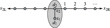
Figure 1: The T-shaped quantum dot model. The gray area represents the quantum dot.

A quantity associated with irreversible behavior is the “survival” probability, which is the probability that the electron, when placed at a specific site at $t=0$, remains there for $t\neq 0$. Hereafter we will choose this site as $d_{1}$. In this case, for some parameters of the system, the survival probability decays almost exponentially for $t>0$ as $t$ increases. This introduces an apparent distinction between past and future, namely the arrow of time, because exponential growth (the opposite of decay) is not observed unless very special initial conditions are chosen.

In the remainder of this section we will present the details of our model. The complete Hamiltonian for the model shown in Fig. 1 is given by

$$H \equiv\sum_{i=1}^{2}\varepsilon_{i}|d_{i}\rangle\langle d_{i}|-g\left(|d_{1}\rangle\langle d_{2}|+|d_{2}\rangle\langle d_{1}|\right)$$

$$-b\sum_{\alpha=L}^{R}\sum_{x=1}^{\infty}\left(|x_{\alpha}+1\rangle\langle x_{\alpha}|+|x_{\alpha}\rangle\langle x_{\alpha}+1|\right)$$

$$-\sum_{\alpha=L}^{R}t_{2\alpha}\left(|1_{\alpha}\rangle\langle d_{2}|+|d_{2}\rangle\langle 1_{\alpha}|\right),$$ (8)

where $|d_{i}\rangle$ denotes the state for which the electron is at site $d_{i}$ in the dot, $|x_{\alpha}\rangle$ denotes the electron being at the $x^{\rm th}$ site of $\alpha^{\rm th}$ lead (with $\alpha=L$ or $R$), $\varepsilon_{i}$ are the chemical potentials at the sites $d_{i}$, $g$ is the coupling between the sites $d_{1}$ and $d_{2}$, $t_{2\alpha}$ is the coupling between the site $d_{2}$ and the $\alpha^{\rm th}$ lead, and $b$ is the inter-site coupling for both leads. We assume that all parameters are real. We will also assume that all the states appearing in the Hamiltonian are even with respect to time-inversion; hence, we have $[H,T]=0$.

The dispersion relation on either lead is

$$E_{k}=-b(e^{ik}+e^{-ik})=-2b\cos k,$$ (9)

where $-\pi<k\leq\pi$ is the wave number limited to the first Brillouin zone. Because the number of degrees of freedom on the leads is countable infinity, the wave number is limited to the Brillouin zone and the energy band has an upper bound in addition to the usual lower bound.

The sites $|d_{1}\rangle$ and $|d_{2}\rangle$ are mathematically analogous to excited and ground states, respectively, of a two-level atom, whereas the leads are analogous to a radiation field that can be emitted from and absorbed into the atom.

Introducing the states $|k_{\alpha}\rangle$ such that $\langle x_{\alpha^{\prime}}|k_{\alpha}\rangle=\delta_{\alpha,\alpha^{\prime}}\sqrt{2}\sin(kx)$, the Hamiltonian is written as $H=H_{0}+H_{1}$, where

$$H_{0} =\sum_{i=1}^{2}\varepsilon_{i}|d_{i}\rangle\langle d_{i}|-g\left(|d_{1}\rangle\langle d_{2}|+|d_{2}\rangle\langle d_{1}|\right)$$

$$+\sum_{\alpha=L}^{R}\int_{-\pi}^{\pi}\frac{dk}{2\pi}E_{k}|k_{\alpha}\rangle\langle k_{\alpha}|,$$ (10)

$$H_{1} =-\sum_{\alpha=L}^{R}t_{2\alpha}\int_{-\pi}^{\pi}\frac{dk}{2\pi}\sqrt{2}\sin(k)\left[|d_{2}\rangle\langle k_{\alpha}|+|k_{\alpha}\rangle\langle d_{2}|\right].$$ (11)

The Hamiltonian can then be diagonalized as follows Newton (1960, 1982):

$$H= \sum_{n\in\mbox{\scriptsize bound}}|\phi_{n}\rangle E_{n}\langle\phi_{n}|+\sum_{\alpha=L}^{R}\int_{-\pi}^{\pi}\frac{dk}{2\pi}|\phi_{k\alpha}\rangle E_{k}\langle\phi_{k\alpha}|.$$ (12)

The first summation runs over all bound eigenstates $|\phi_{n}\rangle$ with eigenvalues $E_{n}$, while $|\phi_{k}\rangle$ denotes the continuum scattering eigenstates with eigenvalues $E_{k}$. The scattering eigenstates have the following well-known expression:

$$|\phi_{k\alpha}\rangle=|{k_{\alpha}}\rangle+\frac{1}{E_{k}-H+i0}H_{1}|{k_{\alpha}}\rangle.$$ (13)

The bound states are residues of the scattering eigenstates at the eigenvalues $E_{n}$.

In addition to the continuous eigenvalues $E_{k}$, the Hamiltonian has four discrete eigenvalues: two bound-state eigenvalues, included in Eq. (12), and either a pair of real eigenvalues corresponding to anti-bound states or a pair of complex-conjugate eigenvalues, corresponding to resonant and anti-resonant states; for concise reviews of resonant and anti-resonant states, see Appendix A of the present article as well as Section II of Ref. Hatano and Ordonez (2014). The transition from real to complex eigenvalues occurs at the exceptional point (EP) as the energy at site $d_{1}$ is increased, as exemplified in Fig. 2.

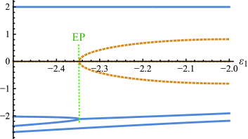
Figure 2: The real (blue solid line) and imaginary (orange broken line) parts of the discrete eigenvalues of the Hamiltonian as functions of the chemical potential $\varepsilon_{1}$ at site $d_{1}$. The imaginary part has been multiplied by $5$ for easier visualization. The vertical dotted line indicates the exceptional point (EP), where a pair of anti-bound (real) eigenvalues in the region left to the EP coalesce to form a resonance-anti-resonance pair of complex-conjugate eigenvalues in the region to the right of the EP. The bound-state eigenvalues form the top and bottom lines. The parameters of the quantum dot are $\varepsilon_{2}=0$, and $g=0.4$, all in units of the inter-site coupling of the leads, $b$, which we set equal to the couplings between the dot and each of the two leads: $t_{2L}=t_{2R}=b=1$.

The appearance of two complex eigenvalues makes the breaking of time-reversal symmetry possible Garmon et al. (2012), if either one of the eigenvalues is selected to generate the time evolution. In Section VII we will show that such selection occurs automatically, although the system remains T-invariant.

IV Survival amplitude

The survival probability of the ‘excited state’ $|d_{1}\rangle$ is given by $P(t)=|A(t)|^{2}$, where $A(t)$ is the survival amplitude:

$$A(t)\equiv\langle d_{1}|e^{-iHt}|d_{1}\rangle=\sum_{n\in\mbox{\scriptsize bound}}\langle d_{1}|\phi_{n}\rangle e^{-iE_{n}t}\langle\phi_{n}|d_{1}\rangle$$

$$+\sum_{\alpha=L}^{R}\int_{-\pi}^{\pi}\frac{dk}{2\pi}\langle d_{1}|\phi_{k\alpha}\rangle e^{-iE_{k}t}\langle\phi_{k\alpha}|d_{1}\rangle,$$ (14)

which follows from Eq. (12). As shown in Appendix B, introducing the variable $\lambda=e^{ik}$ such that $E=-b(\lambda+\lambda^{-1})$, we can express the survival amplitude in the form

$$A(t)=\int_{C}\frac{d\lambda}{2\pi i\lambda}\left(-\lambda+\frac{1}{\lambda}\right)e^{ib\left(\lambda+\frac{1}{\lambda}\right)t}\frac{bg^{2}}{h(\lambda)}\frac{1}{f(\lambda)},$$ (15)

where

$$f(\lambda) =\left[-b\left(\lambda+\frac{1}{\lambda}\right)-\varepsilon_{1}\right]$$

$$\times\left[-b\left(\lambda+\frac{1}{\lambda}\right)-\varepsilon_{2}+\lambda\sum_{\alpha}\frac{t_{2\alpha}^{2}}{b}\right]-g^{2},$$ (16)

$$h(\lambda)\equiv-b\left(\lambda+\frac{1}{\lambda}\right)-\varepsilon_{1},$$ (17)

and the contour $C$ is shown in Fig. 3; we have assumed that the model is in such a parameter region that $f(\lambda)$ has a pair of complex-conjugate roots $\lambda_{R}$ and $\lambda_{AR}$ corresponding to resonance and anti-resonance poles, respectively, and two real roots $\lambda_{B1}$ and $\lambda_{B2}$ corresponding to the two bound states, namely in the region to the right of the EP in Fig. 2. As shown in Appendix C, the poles of $h(\lambda)$ do not contribute to the integral.

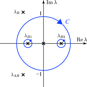
Figure 3: The contour $C$ used in Eq. (15). It includes the unit circle and integrations around the bound-state poles $\lambda_{B1}$ and $\lambda_{B2}$. Also shown are the resonance ($\lambda_{R}$) and anti-resonance ($\lambda_{AR}$) poles as well as the pole at the origin.

When $t>0$ in Eq. (15), we can deform the contour $C$ in Fig. 3 so that we may isolate the contribution from the residue resonant pole $\lambda_{R}$ as shown in Fig. 4(a):

$$A(t)=\langle d_{1}|\phi_{R}\rangle e^{-iE_{R}t}\langle{\tilde{\phi}}_{R}|d_{1}\rangle$$

$$+\int_{C^{\prime}}\frac{d\lambda}{2\pi i\lambda}\left(-\lambda+\frac{1}{\lambda}\right)e^{ib\left(\lambda+\frac{1}{\lambda}\right)t}\frac{bg^{2}}{h(\lambda)}\frac{1}{f(\lambda)},$$ (18)

The first term is the residue at $\lambda_{R}$ and is written in terms of the right and left resonant eigenstates of the Hamiltonian, $|\phi_{R}\rangle$ and $\langle{\tilde{\phi}}_{R}|$ respectively, which satisfy

$$H|\phi_{R}\rangle=E_{R}|\phi_{R}\rangle,\qquad\langle{\tilde{\phi}}_{R}|H=\langle{\tilde{\phi}}_{R}|E_{R},$$ (19)

where $E_{R}=-b(\lambda_{R}+{\lambda_{R}}^{-1})$ is equal to the complex resonance energy.

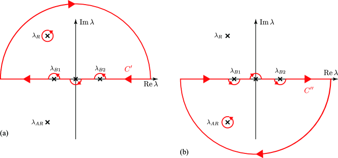
Figure 4: (a) The deformed contour $C^{\prime}$ used in Eq. (IV) for $t>0$. It consists of the real axis going around the origin and the real poles $\lambda_{B1}$ and $\lambda_{B2}$ as well as the infinitely large half circle in the upper half plane. Also shown is the integration around the resonance pole $\lambda_{R}$, which gives the first term in the right-hand-side of Eq. (IV). (b) The deformed contour $C^{\prime\prime}$ that should be used for $t<0$.

These states are normalized such that $\langle{\tilde{\phi}}_{R}|\phi_{R}\rangle=1$, but they are not in the Hilbert space because the Hilbert norms $\langle{\phi}_{R}|\phi_{R}\rangle$ or $\langle{\tilde{\phi}}_{R}|{\tilde{\phi}}_{R}\rangle$ diverge Petrosky et al. (1991). It is worth noting that although these states grow exponentially in space representation, the normalization constant giving $\langle{\tilde{\phi}}_{R}|\phi_{R}\rangle=1$ can be obtained by adding a convergence factor, as shown in Appendix D of Ref. Hatano and Ordonez (2014).

Since the energy eigenvalue $E_{R}$ has a negative imaginary part, the first term in Eq. (IV) represents an exponential decay for $t>0$. The anti-resonant eigenstate (associated with the anti-resonant pole) is the complex conjugate of the resonant eigenstate as $|\phi_{AR}\rangle=|\phi_{R}\rangle^{*}$, which, however, does not explicitly contribute to Eq. (IV). The contributions from both the infinitesimal half circle around the origin and the infinite half circle in the upper half plane vanish for $t>0$ because of the exponential factor in the integrand, which is indeed the motivation for modifying the contour to $C^{\prime}$ in the first place. The integration on the real axis in Fig. 4 can be evaluated by different approximations, for example the saddle-point approximation for large $t$ Hatano and Ordonez (2014) (see also Appendix F) or the short-time approximation in Section VIII.

When $t<0$ in Eq. (15), we are compelled to deform the contour as shown in Fig. 4(b), because contributions from both the infinitesimal half circle around the origin and the infinite half circle in the lower half plane vanish for $t<0$. After the contour deformation we obtain

$$A(t)=\langle d_{1}|\phi_{AR}\rangle e^{-iE_{AR}t}\langle{\tilde{\phi}}_{AR}|d_{1}\rangle$$

$$+\int_{C^{\prime\prime}}\frac{d\lambda}{2\pi i\lambda}\left(-\lambda+\frac{1}{\lambda}\right)e^{ib\left(\lambda+\frac{1}{\lambda}\right)t}\frac{bg^{2}}{h(\lambda)}\frac{1}{f(\lambda)}.$$ (20)

Now the anti-resonant pole contributes instead of the resonant pole. Since the energy eigenvalue $E_{AR}$ has a positive imaginary part, the first term in Eq. (IV) grows exponentially as negative $t$ increases, approaching the origin. The integration over the real axis can be evaluated by the same approximations used for the $t>0$ case.

Note that these countour deformations are the most natural choice for the evaluation of the integral in the respective cases of $t>0$ and $t<0$ because we should nullify the essential singularities at $\lambda=0$ and $|\lambda|=\infty$. We will show in Section VI by numerically evaluating the integral that the above arguments indeed give the correct behavior.

V Previous approach: Breaking time-reversal invariance by hand

In this section we will summarize the previous approach Prigogine et al. (1973); Petrosky et al. (1991); Petrosky and Prigogine (1996, 1997); Ordonez et al. (2001); Petrosky et al. (2001) for obtaining irreversible equations, using our model as a simple example.

The main idea is to isolate terms like the first term in Eq. (IV), which break T-invariance. To do this, we introduce the projection operators $P_{1}\equiv|d_{1}\rangle\langle d_{1}|$, $\Pi_{R}\equiv|\phi_{R}\rangle\langle{\tilde{\phi}}_{R}|$ and ${\check{\Pi}}_{R}=1-\Pi_{R}$. Then Eq. (IV) may be written as

$$A(t)=\langle d_{1}|\xi_{R}(t)\rangle+\langle d_{1}|{\check{\xi}}_{R}(t)\rangle,$$ (21)

where the states

$$|\xi_{R}(t)\rangle=P_{1}\Pi_{R}e^{-iE_{R}t}|d_{1}\rangle,$$ (22)

$$|{\check{\xi}}_{R}(t)\rangle=P_{1}{\check{\Pi}}_{R}e^{-iHt}|d_{1}\rangle$$ (23)

correspond to the first and second terms in Eq. (IV), respectively.

The state $|\xi_{R}(t)\rangle$ breaks the T-invariance because by applying $T^{2}=1$ to it and using the antisymmetry of $T$ we obtain

$$|\xi_{R}(t)\rangle=Te^{iE_{R}^{*}t}TP_{1}\Pi_{R}|d_{1}\rangle\neq Te^{iE_{R}t}TP_{1}\Pi_{R}|d_{1}\rangle,$$ (24)

which violates Eq. (2). The reason is that the generator of motion in Eq. (22) is not the Hamiltonian; it is $E_{R}$, which is complex and no longer commutes with the $T$ operator.

However, the complete time evolution is T-invariant, because it is generated by the Hamiltonian. This means that the second term in Eq. (IV) must also break the T-invariance in such a way that the complete quantity satisfies T-invariance.

The state $|\xi_{R}(t)\rangle$ makes physical sense when $t>0$. As shown in Fig. 5, it becomes unphysical for $t<0$, however, because the projected component of the survival probability then grows exponentially, unbounded, as $t$ becomes more negative. To avoid this, for $t<0$ we have to extract the residue at the anti-resonance pole $\lambda_{AR}$ instead of $\lambda_{R}$. Doing this will lead to exponential decay towards the past as $t$ becomes more negative. Alternatively, we can say that in this case the condition at $t=0$ is a final condition (rather than an initial condition) and for $t<0$ the survival amplitude grows exponentially as it approaches the terminal condition at $t=0$. In order for it not to grow unbounded when $t$ becomes positive, we must switch the pole that we isolate from the anti-resonant pole $\lambda_{AR}$ to the resonant pole $\lambda_{R}$ at $t=0$.

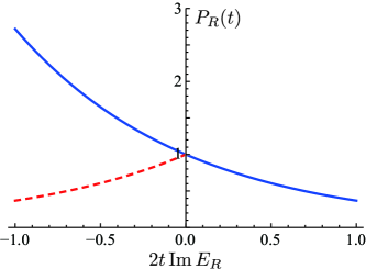
Figure 5: Solid line: the resonance component of the survival probability $P_{R}(t)=\left|\langle d_{1}|\xi_{R}(t)\rangle\right|^{2}$. Dashed line: the anti-resonance component for $t<0$.

Thus, in summary, the survival amplitude may be decomposed as a sum of terms that break T-invariance individually but added together are T-invariant as is shown in Eq. (21). To obtain the proper direction of the growth and the decay, we picked up a pole “by hand.” If the system has more than one pair of complex-conjugate eigenvalues, it becomes somewhat arbitrary which poles we pick; the separation of irreversible components is in general not unique. Moreover, the irreversible components can become unphysical. An example of this is the $\Pi_{R}$ component of the initial state becoming unphysical for $t<0$.

In the following section we will present our new formulation, which relies on a T-symmetric decomposition, yet nevertheless reveals the emergence of irreversible behavior.

VI Present approach: The T-symmetric formulation

We will express the survival amplitude of the ‘excited state’ $|d_{1}\rangle$ using the result of the quadratic-eigenvalue-problem (QEP) formalism discussed in Ref. Hatano and Ordonez (2014). As shown in Ref. Hatano and Ordonez (2014), the survival amplitude (IV) is also expanded in the form

$$A(t) =\sum_{n=1}^{2N}\langle d_{1}|\chi_{n}(t)\rangle$$ (25)

with

$$|\chi_{n}(t)\rangle =\frac{1}{2\pi i}\int_{C}d\lambda\,\left(-\lambda+\frac{1}{\lambda}\right)\exp\left[ib\left(\lambda+\frac{1}{\lambda}\right)t\right]$$

$$\times|\psi_{n}\rangle\frac{\lambda_{n}}{\lambda-\lambda_{n}}\langle\tilde{\psi}_{n}|d_{1}\rangle.$$ (26)

Note that $N=2$ in the present case, which is the number of sites of the dot in the gray area of Fig. 1.

The integration contour $C$ is shown in Fig. 3. The summation over $n$ includes resonant, anti-resonant, and bound eigenstates of the Hamiltonian. The states $|\psi_{n}\rangle$ and $\langle\tilde{\psi}_{n}|$ are the corresponding right and left eigenstates of the Hamiltonian with eigenvalues $E_{n}=-b(\lambda_{n}+{\lambda_{n}}^{-1})$. They have a different normalization than the eigenstates $|\phi_{n}\rangle$ used in Section IV as in

$$|\phi_{n}\rangle=(1-\lambda_{n}^{2})^{1/2}|\psi_{n}\rangle.$$ (27)

For the present model, Eq. (25) can also be obtained from Eq. (15) using a partial-fraction expansion of the integrand; see Appendix C. Note, however, the essential difference between the expressions (IV) and (25). The former (Eq. (IV)) is expanded in terms of the well-known complete set that consists of the bound states and the scattering states, in other words, all states on the first Riemann sheet Newton (1960, 1982). We expanded the latter (Eq. (25)) in terms of our new complete set which consists of all point spectra on the first and second Riemann sheets, namely the bound, anti-bound, resonant and anti-resonant states Hatano and Ordonez (2014).

Instead of separating the pole contributions in the integral over $\lambda$, we will simply evaluate the integral over $\lambda$ for each component of the summation in Eq. (25), individually. The eigenstate components such as $\langle d_{1}|\psi_{n}\rangle$ can be calculated using the method given in Section VII, Eq. (74) of Ref. Hatano and Ordonez (2014).

Figure 6 shows the numerically evaluated contributions $|\langle d_{1}|\chi_{n}(t)\rangle|^{2}$ to the survival probability corresponding to the resonant, anti-resonant and bound eigenstates. It is seen that separately, the resonant and anti-resonant contributions are not even functions of time; we will show that they violate condition (5) for T-invariance. However, taken as a whole the sum $\left|\langle d_{1}|\chi_{\rm R}(t)\rangle+\langle d_{1}|\chi_{\rm AR}(t)\rangle\right|^{2}$ adds up to a T-invariant evolution and produce an even function of time.

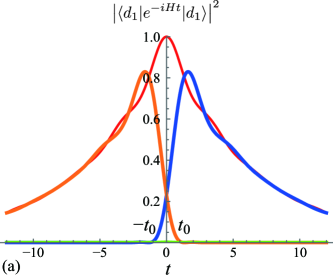
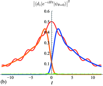
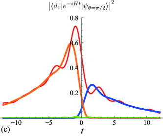
Figure 6: (a) Contributions to the total survival probability $|A(t)|^{2}$ of the ‘excited state’ (red line with the highest peak) corresponding to: the resonant state $|\langle d_{1}|\chi_{R}(t)\rangle|^{2}$ (blue line with a lower peak on the right); the anti-resonant state $|\langle d_{1}|\chi_{AR}(t)\rangle|^{2}$ (yellow line with a lower peak on the left) and bound states $|\langle d_{1}|\chi_{B}(t)\rangle|^{2}$ (green line almost indistinguishable from the horizontal axis). We here plot as the contributions the square modulus of each component, which do not add up to the plotted total survival probability. The parameters are $b=1$, $\varepsilon_{1}=0.2$, $\varepsilon_{2}=0$, $g=0.4$, and $t_{2L}=t_{2R}=1$. Similarly, the probability $\left|\langle d_{1}|\psi_{\theta}(t)\rangle\right|^{2}$ with $|\psi_{\theta}(0)\rangle$ given by Eq. (31), (b) for $\theta=0$ and (c) for $\theta=\pi/2$. For $\theta=\pi/2$ the resonant and anti-resonant components of the state $|\psi_{\theta}(0)\rangle$ have different weights.

We remark that in contrast to the isolated resonant pole contribution discussed in Section V, the curve of the resonant contribution in Fig. 6 does not have an unbounded exponential growth for $t<0$; compare Fig. 7(a) with Fig. 5. Similarly, the curve of the anti-resonant contribution does not grow exponentially for $t>0$. Furthermore, the resonant or anti-resonant components are free from any unbounded exponential growth in the position representation García-Calderón (2010); Hatano and Ordonez (2014), whereas the non-Hilbertian states $|\phi_{R}\rangle$ of $\langle{\tilde{\phi}}_{R}|$ diverge exponentially in position representation; see Fig. 7(b). We stress that the present decomposition (25) produces the automatic switching around $t=0$ from the anti-resonant contribution that grows for negative time to the resonant contribution that decays for positive time; we do not switch them by hand. Another marked difference from the approach in Section V is the fact that the anti-resonant contribution does not suddenly give way to the resonant contribution; this will be the central topic of Section VIII.

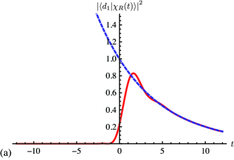
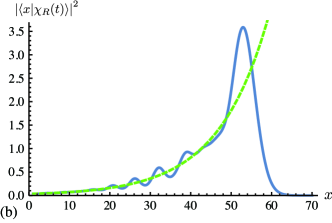
Figure 7: (a) The resonant component of the survival probability, $\left|\langle d_{1}|\chi_{R}(t)\rangle\right|^{2}$ (solid line) compared to the non-Hilbert state component $\left|\langle d_{1}|\phi_{R}(t)\rangle\right|^{2}$ (dashed line). The parameters are the same as in Fig. 6. (b) The resonant component $\left|\langle x|\chi_{R}(t)\rangle\right|^{2}$ (solid line) compared to the non-Hilbert state component $\left|\langle x|\phi_{R}(t)\rangle\right|^{2}$ (dashed line) in the position representation. This figure is similar to Fig. 7.11 in Ref. García-Calderón (2010) or Fig. 2 in Ref. Petrosky et al. (2001), although the latter two display the complete probability density in space representation rather than the resonance component alone.

To formulate the breaking of T-invariance for the individual components of Eq. (25), we consider the effect that the time-reversal operator has on each component (VI). Applying $T$ to these states takes the complex conjugate of all constants. Taking the complex conjugate of $\lambda$ changes $\lambda\to\lambda^{-1}$ around the unit circle, whereas $\lambda$ remains unchanged on the infinitesimal circles around the bound-state poles. We can bring $\lambda$ back to its initial form by making the change of variables $\lambda\to\lambda^{-1}$. Then we have

$$T|\chi_{n}(t)\rangle =\frac{1}{2\pi i}\int_{C}d\lambda\,\left(-\lambda+\frac{1}{\lambda}\right)\exp\left[-ib\left(\lambda+\frac{1}{\lambda}\right)t\right]$$

$$\times|\psi_{n}\rangle^{*}\frac{\lambda_{n}^{*}}{\lambda-\lambda_{n}^{*}}\langle\tilde{\psi}_{n}|d_{1}\rangle^{*}.$$ (28)

Here the resonant and anti-resonant states, $|\psi_{R}\rangle$ and $|\psi_{AR}\rangle=|\psi_{R}\rangle^{*}$, are complex, while the bound-state components are real. Therefore we have

$$T|\chi_{R}(t)\rangle=|\chi_{AR}(-t)\rangle,$$

$$T|\chi_{AR}(t)\rangle=|\chi_{R}(-t)\rangle,$$

$$T|\chi_{B}(t)\rangle=|\chi_{B}(-t)\rangle,$$ (29)

where $B$ represents a bound state. We see that due to complex conjugation, the resonant and anti-resonant states break T-invariance, while the bound states do not (compare Eq. (VI) with Eq. (5)). However, the summation of resonant and anti-resonant components satisfies T-invariance:

$$T\left(|\chi_{R}(t)+|\chi_{AR}(t)\rangle\right)=\left(|\chi_{R}(-t)+|\chi_{AR}(-t)\right).$$ (30)

So far, we have considered the decay of the ‘excited state,’ choosing $|d_{1}\rangle$ as the initial state, but we can also consider an initial state of the form

$$|\psi_{\theta}(0)\rangle=\frac{1}{\sqrt{2}}\left(|d_{1}\rangle+e^{i\theta}|d_{2}\rangle\right),$$ (31)

which is generally not even with respect to time-inversion. Under the time reversal we have

$$\langle d_{1}|T|\psi_{\theta}(t)\rangle=\langle d_{1}|Te^{-iHt}|\psi_{\theta}(0)\rangle=\langle d_{1}|\psi_{-\theta}(-t)\rangle$$ (32)

Thus, from Eq. (6) we obtain

$$\langle d_{1}|\psi_{-\theta}(-t)\rangle=\langle d_{1}|\psi_{\theta}(t)\rangle^{*},$$ (33)

which means that the probability $\left|\langle d_{1}|\psi_{\theta}(t)\rangle\right|^{2}$ is no longer an even function of time, unless $\theta=0$ or $\theta=\pi$. This is demonstrated in Fig. 6 (b) and (c).

The components of $|\psi_{\theta}(t)\rangle$,

$$|\chi_{n}(t,\theta)\rangle =\frac{1}{2\pi i}\int_{C}d\lambda\,\left(-\lambda+\frac{1}{\lambda}\right)\exp\left[ib\left(\lambda+\frac{1}{\lambda}\right)t\right]$$

$$\times|\psi_{n}\rangle\frac{\lambda_{n}}{\lambda-\lambda_{n}}\langle\tilde{\psi}_{n}|\psi_{\theta}\rangle,$$ (34)

satisfy

$$\langle d_{1}|\chi_{\rm R}(t,\theta)\rangle=\langle d_{1}|\chi_{\rm AR}(-t,-\theta)\rangle^{*}$$ (35)

and

$$\langle d_{1}|\chi_{\rm B}(t,\theta)\rangle=\langle d_{1}|\chi_{\rm B}(-t,-\theta)\rangle^{*},$$ (36)

which shows that the bound-state components and the sum of resonance and anti-resonance components of the probability are even functions of time only if $\theta=0$ or $\theta=\pi$.

VII Automatic breaking of resonance-antiresonance symmetry

Despite the symmetry of the survival probability around $t=0$ in Fig. 6(a), we can still say that the exponential decay process has an irreversible nature; starting at the dot $d_{1}$ at $t=0$, for $t>0$ the electron enters the infinite wire and never comes back. (The same could be phrased for $t<0$ but in this context we usually do not say that an electron moves backward in time.)

In the following, we will argue that this irreversible nature emerges as a breaking of the resonance-antiresonance symmetry that exists in the initial state, which we assume is invariant under time inversion, namely $T|\psi(0)\rangle=|\psi(0)\rangle$. As a result of this invariance, the resonant and anti-resonant components of the survival amplitude have equal magnitudes at $t=0$. For example, when the initial state is $|d_{1}\rangle$ we have $\langle d_{1}|\chi_{R}(0)\rangle=\langle d_{1}|\chi_{AR}(0)\rangle^{*}$. The initial state thus has a resonance-antiresonance symmetry.

However, this symmetry is automatically broken by time evolution, as seen in Fig. 6(a). The figure shows that for $t>0$ the anti-resonant component is significantly suppressed after a time $t_{0}$. Figure 6(a) also shows that, as the anti-resonance component becomes negligible for $t>0$, the whole survival probability (red line with the highest peak) approaches the contribution due to the resonant component alone (blue line with a lower peak on the right), which breaks T-invariance by itself. In this way the complete time evolution mimics the time evolution of the strictly irreversible resonant component.

Note that in the example that we are considering there are no other resonance/anti-resonance pairs and, moreover, the bound states give a negligible contribution. For more complicated systems, there can be more than one resonance/anti-resonance pair; the breaking of resonance-antiresonance symmetry would then manifest itself within each pair, as the time evolution alone would suppress one component of the pair relative to the other component. The bound-state contributions (even if they are not negligible) are only trivially affected by the $T$ operator, since they satisfy T-invariance by themselves, i.e., $\langle d_{1}|\chi_{\rm B}(t)\rangle=\langle d_{1}|\chi_{\rm B}(-t,)\rangle^{*}$.

To quantify the extent of resonance-antiresonance symmetry breaking, we consider the ratio of the resonant-state contribution to the anti-resonant state contribution within the pair:

$$r=\left|\frac{\langle d_{1}|\chi_{R}(t)\rangle}{\langle d_{1}|\chi_{AR}(t)\rangle}\right|^{2}=\left|\frac{\langle d_{1}|\chi_{R}(t)\rangle}{\langle d_{1}|\chi_{R}(-t)\rangle}\right|^{2}.$$ (37)

If the resonance-antiresonance symmetry were completely broken, then $r$ would be $\infty$ for $t>0$ and $0$ for $t<0$.

Note that at $t=0$ we have $r=1$; this reflects the invariance of the state $|d_{1}\rangle$ with respect to time reversal. However, as $t$ increases the ratio quickly jumps from $r=1$ at $t=0$ to a large value, as shown in Fig. 8(a), meaning that the resonant-state contribution becomes much larger than the anti-resonant contribution.

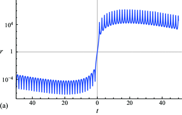
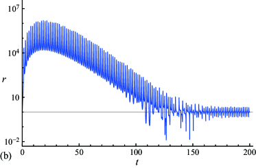
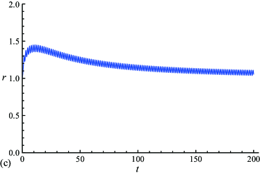
Figure 8: (a) The ratio $r$ of the resonant component of the survival probability to the anti-resonant component in a semi-logarithmic scale. The parameters are the same as in Fig. 6. (b) The same in a longer time scale. (c) The ratio with $\varepsilon_{1}$ changed to $-2.347528$, when the pair of resonant and anti-resonant poles are near an exceptional point. The rapid oscillations seen in all the figures have a period inversely proportional to the band-edge energies with $|E|=2$ (see Eq. (108)).

This jump in $r$ occurs around the time $t=t_{0}\simeq 1$, which we will relate to the system parameters in Section VIII. Conversely, the anti-resonant contribution dominates for $t<-t_{0}$. For both positive or negative times, the larger $\left|\log r\right|$ is, the more the time evolution approaches a complete breaking of resonance-antiresonance symmetry. We stress again that since the time evolution alone suppresses the anti-resonances for $t>t_{0}$ (and the resonances for $t<-t_{0}$), we do not have to isolate the resonance or anti-resonance contributions by hand. This happens automatically.

We remark that for very long time the regime of exponential decay is known to be replaced by the “long-time regime” of an inverse power-law decay Garmon et al. (2013). Indeed, the ratio (37) settles back to unity as shown in Fig. 8(b), which indicates that the irreversible behavior disappears at very long-time scales. This is proved in Appendix F.

Another remark is that if the chemical potentials $\varepsilon_{i}$ of the impurity are adjusted, the pair of the resonant and anti-resonant eigenvalues (in the region right of the EP in Fig. 2) can approach the exceptional point (EP), where these eigenvalues converge into a single real energy and subsequently split into two anti-bound real eigenvalues Garmon et al. (2012) (in the region left of the EP in Fig. 2), which satisfy T-invariance individually. As shown in Fig. 8(c), when the resonance and anti-resonance pair is near the EP, the change of the ratio $r$ is much less dramatic than in Fig. 8(a). The time evolution then hardly has irreversible nature, because both the resonant and anti-resonant components have significant weight throughout the whole time evolution.

When there are no resonant and anti-resonant pairs, only bound and anti-bound states (i.e., to the left of the EP in Fig. 2), then there is no breaking of resonance-antiresonance symmetry to speak of; the system has no irreversible behavior then.

VIII Time scale for the breaking of resonance-antiresonance symmetry

In Fig. 6(a), it is seen that the resonant-state contribution to the survival amplitude does not jump discontinuously at $t=0$; instead it is a continuous function of time: it increases gradually starting at a negative time $-t_{0}$, then it reaches a peak after $t=0$ and eventually decays exponentially. Similarly, the antiresonance-state contribution does not suddendly disappear for positive times; instead, it leaks into the postive-time region and becomes negligible after the positive time $t_{0}$. The time range $[-t_{0},t_{0}]$ is a time region during which the resonance-antiresonance is unbroken; outside of this range the symmetry is broken. In the following, we will estimate the magnitude of the time $t_{0}$, which will turn out to be close to the Zeno time (note that our present model does not include monitoring; the connection with the Zeno time will be done based on the conditions that the unmeasured survivival probability must meet for the Zeno effect to occur).

In Appendix D we derive the following analytic expression for the resonant component of the survival amplitude:

$$A_{{\rm R}}(t)=\langle d_{1}|\chi_{R}(t)\rangle=\langle d_{1}|\psi_{R}\rangle\langle\tilde{\psi}_{R}|d_{1}\rangle$$

$$\times e^{-iE_{R}t}\left[1-i\lambda_{R}\int_{0}^{t}dt^{\prime}\,e^{iE_{R}t^{\prime}}\frac{J_{1}(2bt^{\prime})}{t^{\prime}}\right],$$ (38)

which can also be written as

$$A_{{\rm R}}(t)=\langle d_{1}|\phi_{R}\rangle\langle\tilde{\phi}_{R}|d_{1}\rangle$$

$$\times e^{-iE_{R}t}\left[1+\frac{i\lambda_{R}}{1-\lambda_{R}^{2}}\int_{t}^{\infty}dt^{\prime}\,e^{iE_{R}t^{\prime}}\frac{J_{1}(2bt^{\prime})}{t^{\prime}}\right];$$ (39)

see Appendix E. The former expression (VIII) is useful to calculate the short-time evolution, whereas the latter (VIII) is useful for long times. We remark that the first term in brackets in Eq. (VIII) gives the resonant eigenstate projection $\Pi_{R}$ discussed in Section V.

Hereafter we will only use Eq. (VIII). We will estimate the time it takes for the time-evolved state $|d_{1}\rangle$ to approach the irreversible evolution due to the resonant state alone. We start with the following short-time approximation: $J_{1}(2bt)\approx bt$. The resonant component of the survival probability is then given by

$$P_{R}(t)=\left|A_{R}(t)\right|^{2}$$

$$\approx\left|\langle d_{1}|\psi_{\rm R}\rangle\langle\tilde{\psi}_{\rm R}|d_{1}\rangle e^{-iE_{\rm R}t}\left[1-\frac{b\lambda_{\rm R}}{E_{\rm R}}\left(e^{iE_{\rm R}t}-1\right)\right]\right|^{2}.$$ (40)

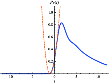
Figure 9: Solid line: exact contribution of the resonant state to the survival probability. Dashed line: approximation valid for short time. Parameters are $b=1,\varepsilon_{1}=0.2,\varepsilon_{2}=0,g=0.4,t_{2L}=t_{2R}=1$. For these parameters we have $E_{\rm R}=0.199675-0.0803343i$, $\lambda_{\rm R}=-0.103865+1.03599\,i$ and $|\lambda_{\rm R}|=1.04118$.

Figure 9 shows a numerical plot of the resonant-state contribution to the survival probability as a function of time. The solid line is the exact expression, while the dashed line shows the short-time approximation, Eq. (VIII). It is seen that the short-time approximation is close to zero for a negative time $-t_{0}$. For times earlier than $-t_{0}$, the exact probability $P_{\rm R}(t)$ is approximately zero and the anti-resonance contribution dominates (see Fig. 6). Conversely, for times larger than $+t_{0}$, the anti-resonance contribution vanishes, and the resonance contribution dominates. Therefore the time $t_{0}$ gives the time scale of breaking of resonance-antiresonance symmetry.

To find $-t_{0}$ we will assume that the imaginary part of the resonance energy is much smaller than its real part:

$$\left|\operatorname{\mathrm{Im}}E_{{\rm R}}\right|\ll\left|\operatorname{\mathrm{Re}}E_{{\rm R}}\right|.$$ (41)

In this case, and assuming $|E_{\rm R}|<2b$, we have $|\lambda_{\rm R}|\approx 1$, which is true for the parameters used in Fig. 9.

Under the assumption (41), we set Eq. (VIII) equal to zero to arrive at

$$-t_{0}=\frac{2\log(\lambda_{\rm R})-\pi i}{-iE_{\rm R}}.$$ (42)

This expression is approximately real because the energy $E_{\rm R}$ is approximately real and $\log(\lambda_{\rm R})$ is approximately pure imaginary. Note that as long as (41) is satisfied, $t_{0}$ is independent of $\operatorname{\mathrm{Im}}E_{{\rm R}}$.

It is interesting to compare $t_{0}$ with the “Zeno time” $t_{Z}$ discussed in Ref. Petrosky and Barsegov (2002). This time is given by $t_{Z}=1/E$, where $E$ is the unperturbed energy of the excited state. It is of the same order of magnitude as $t_{0}\sim 1/E_{R}$ in Eq. (42). The time $t_{Z}$ marks a transition from early non-exponential decay ($t\lesssim t_{Z}$) to exponential decay ($t\gtrsim t_{Z}$). It is called the Zeno time due to the following connection with the quantum Zeno effect Misra and Sudarshan (1977):

The Zeno effect occurs when, shortly after the excited state is prepared at $t=0$, an experimenter performs repeated measurements at times $\Delta t$, $2\Delta t$, $3\Delta t$, etc., to test whether the state is still excited. If $\Delta t$ is short enough, so that for $|t|<\Delta t$ the survival probability is parabolic, then the repeated measurements “freeze” the survival probability and prevent it from decaying. The time $t_{Z}$ is generally much larger than $\Delta t$, so that $t_{Z}$ gives an upper bound for $\Delta t$; it gives a time boundary beyond which there can be no Zeno effect.

Besides the relation $t_{0}\sim t_{Z}$, there is also the following connection between resonance-antriresonance symmetry and the Zeno effect: the latter can only occur if the time derivative of the unmeasured survival probability vanishes at $t=0$. In terms of our analysis, this occurs due to the cancellation of resonance and antisonance terms that are linear in time. This cancellation is visualized in Fig. 6(a), where the resonance and anti-resonance curves have opposite slopes around $t=0$ while they have about the same magnitude. The Zeno effect then is associated with the existence of an unbroken resonance-antiresonance symmetry. Once the symmetry is broken, the excited state can no longer be frozen by repeated measurements.

We have considered the case in which there is only one pair of resonance and anti-resonance. If there is more than one pair, each pair will have its own time $t_{0}$. We could then consider the ratio of the sum of all the resonance contributions to the sum of all the antiresonance contributions, as a measure of the overall resonance-antiresonance symmetry. This symmetry would be broken after the largest time $t_{0}$, among all the pairs.

We remark that when a resonance is close to a band-edge or to an exceptional point, the non-exponential decay is enhanced Jittoh et al. (2005); García-Calderón and Villavicencio (2006); Garmon et al. (2013); Garmon and Ordonez (2017). For example, the enhancement due to the band edges (when $E_{R}\to\pm 2$ or $\lambda_{R}\to\pm 1$) can be seen in Eqs. (VIII) and (F) as well as Eq. (119) of Ref. Hatano and Ordonez (2014). Figure 8(c) shows that, when the resonance is close to the exceptional point, it never dominates over the anti-resonance; there is never a regime of exponential decay in the survival probability.

In these cases, the anti-resonant component is no longer negligible as compared to the resonant component after the short time scale given by $t_{Z}=1/|E_{R}|$. The time $t_{Z}$ then only gives an upper bound of validity of the short-time approximation in Eq. (VIII).

IX Extension to a spatially-continuous model

The results presented so far were based on a model with discrete space. For models with continuous space, time-reversal symmetric expansions in terms of discrete eigenstates of the Hamiltonian have been studied in Refs. More (1971); García-Calderón (1976); Tolstikhin et al. (1998); Tolstikhin (2006, 2008); García-Calderón (2010); García-Calderón et al. (2012); Brown et al. (2016). In these studies, the Hamiltonian has a scattering potential with compact support. Here we will show that our results for the tight-binding models can be directly extended to models with a discrete state coupled to a continuous space, such as the Friedrichs model Friedrichs (1948) discussed in Ref. Lewenstein and Rzazewski (2000), with Hamiltonian

$$H =\omega_{1}|1\rangle\langle 1|+\sum_{k}\omega_{k}|k\rangle\langle k|$$

$$+\sum_{k}\left(V_{k}|1\rangle\langle k|+V_{k}^{*}|k\rangle\langle 1|\right),$$ (43)

where $-\infty<k<\infty$,

$$\omega_{k}=|k|,$$ (44)

and

$$V_{k}=g\sqrt{\frac{2\pi}{L}\frac{\sqrt{\beta\omega_{k}}}{\omega_{k}+\beta}}.$$ (45)

The survival amplitude $A(t)=\langle 1|e^{-iHt}|1\rangle$ may be expressed as

$$A(t)=\sum_{n\in{\rm bound}}\langle 1|\phi_{n}\rangle e^{-iE_{n}t}\langle\phi_{n}|1\rangle+A_{\rm cut}(t),$$ (46)

where the first term on the right-hand side is the contribution from the bound eigenstates of the Hamiltonian (with eigenvalues $E_{n}$) and the second term is the contribution from the scattering eigenstates, expressed as

$$A_{\rm cut}(t)=\frac{1}{2\pi i}\int_{C}\langle 1|\frac{1}{E-H}|1\rangle e^{-iEt}dE.$$ (47)

Here $C$ is the contour shown in Fig. 10; it surrounds the branch cut of the Green’s function on the complex-energy plane. The Green’s function for real $E$ is given by (see Appendix G)

$$\langle 1|\frac{1}{E-H\pm i0}|1\rangle=\left(E-\omega_{1}+2\pi g^{2}\frac{\beta\pm i\sqrt{\beta E}}{\beta+E}\right)^{-1},$$ (48)

where we use the $+$ sign for the part of the contour $C$ just above the real axis and the $-$ sign for the part just below. We rearrange the Green’s function as follows:

$$\langle 1|\frac{1}{E-H\pm i0}|1\rangle$$

$$=\frac{\beta+E}{(E-\omega_{1})(\beta+E)+2\pi g^{2}(\beta\pm i\sqrt{\beta E})}$$

$$=\frac{(\beta+E)\left((E-\omega_{1})(\beta+E)+2\pi g^{2}(\beta\mp i\sqrt{\beta E})\right)}{\left((E-\omega_{1})(\beta+E)+2\pi g^{2}\beta\right)^{2}+(2\pi g^{2})^{2}\beta E},$$ (49)

where in the last line we multiplied and divided the fraction by the complex conjugate of the denominator. Inserting this expression into Eq. (47) we note that the real part of the Green’s function cancels when we integrate along the contour $C$; thus only the imaginary part remains and we obtain

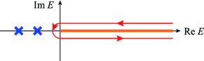
Figure 10: The contour $C$ in Eq. (47). The branch cut of $\sqrt{E}$ lies on the positive real axis, on which also lies the scattering continuum. Bound states can exist on the negative real axis.

$$A_{\rm cut}(t)$$

$$=\int_{0}^{\infty}\frac{2g^{2}(E+\beta)\sqrt{\beta E}e^{-iEt}}{\left[(E+\beta)(E-\omega_{1})+2g^{2}\pi\beta\right]^{2}+(2g^{2}\pi)^{2}\beta E}dE.$$ (50)

Even though the denominator is a quartic polynomial, one of its roots, $E=-\beta$, is not a pole because the numerator vanishes at this point. Therefore there are only three poles, corresponding to a bound-state energy $E_{B}$, a resonance $E_{R}$ and an anti-resonance $E_{AR}=E_{R}^{*}$. Using a partial-fraction expansion we have

$$A_{\rm cut}(t) =\int_{0}^{\infty}\sqrt{\beta E}e^{-iEt}$$

$$\times\left(\frac{W_{B}}{E-E_{B}}+\frac{W_{R}}{E-E_{R}}+\frac{W_{AR}}{E-E_{AR}}\right)dE,$$ (51)

where $W_{AR}=W_{R}^{*}$. The same expansion has been used in Ref. Lewenstein and Rzazewski (2000) to study the anti-Zeno effect. Equation (IX) is analogous to the expansion (25); we can write it as $A_{\rm cut}(t)=\sum_{n}A_{n}(t)$, where

$$A_{n}(t) =\int_{0}^{\infty}\sqrt{\beta E}e^{-iEt}\frac{W_{n}}{E-E_{n}}dE.$$ (52)

Consequently, just as we did with the discrete lattice model, we can decompose the survival amplitude into components that describe the self-generated breaking of resonance-antiresonance symmetry; see Fig. 11.

We can also estimate the time scale for the breaking of resonance-antiresonace symmetry, as follows. The integral in Eq. (52) can be expressed in terms of the complementary error function Lewenstein and Rzazewski (2000):

$$A_{n}(t) =W_{n}\sqrt{\beta}\left[\sqrt{\frac{\pi}{it}}-\pi i\sqrt{E_{n}}e^{-itE_{n}}{\rm erfc}\left(i\sqrt{iE_{n}t}\right)\right].$$ (53)

For $t<0$ and $-t\gg 1/|E_{R}|$ we can use an asymptotic expansion of the complementary error function to obtain for the resonance contribution

$$A_{R}(t) =W_{R}\sqrt{\pi\beta E_{n}}\frac{-i}{2\left(i\sqrt{iE_{R}t}\right)^{3}}\left[1+O\left(\frac{1}{E_{R}t}\right)\right],$$ (54)

which vanishes as $(E_{R}t)^{-3/2}$ for $-t\gg 1/|E_{R}|$. Note that this is not the long-time inverse power decay (e.g., Eq. (F)), which occurs for positive times that are much larger than the lifetime of the resonant state.

Similarly, the anti-resonant contribution vanishes for $t\gg 1/|E_{R}|$. Therefore $1/|E_{R}|$ gives the time scale for the breaking of resonance-antiresonance symmetry. As we discussed in Section VIII, we may call this time scale the “Zeno time” because the Zeno effect occurs within this time scale.

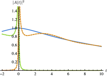
Figure 11: Survival probability $|A(t)|^{2}$ for the Friedrichs model (solid line); resonant-state contribution $\left|A_{R}(t)\right|^{2}$ (dashed line) and antiresonant-state contribution $\left|A_{AR}(t)\right|^{2}$ (dotted line), with the amplitudes $A_{n}(t)$ given in Eq. (52). The bound-state contribution $\left|A_{B}(t)\right|^{2}$ can be barely seen as a small peak around $t=0$; it is an even function of time. The sum of resonant and anti-resonant contributions form an even function of time, but individually they break T-invariance. The parameters used are $\beta=0.5$ and $g=0.1$. For these parameters the resonance energy is $E_{R}=0.98-0.030i$. The time scale for the breaking of resonance-antiresonance symmetry discussed in the text is $1/|E_{R}|=1.02$

X Concluding remarks

In this paper we have described exponential decay in simple open quantum systems, using the T-symmetric expansion in Eqs. (25) and (IX). These expansions include both resonance and antiresonance components in a symmetric way. Starting with these expansions, we did the following:

1. We showed that time-evolution breaks, by itself, the symmetry of the resonance and antiresonance components of a time-reversal invariant initial state. When this symmetry is broken, the time evolution closely matches the irreversible evolution of the isolated remaining component (resonant-state component for $t>0$ or antiresonant-state component for $t<0$).

2. We introduced a parameter ($r$) that quantifies the degree of resonance-antiresonance symmetry breaking in the evolving quantum state. This symmetry is effectively broken when $|\log r|\gg 1$.

3. We estimated the time that it takes for the breaking of resonance-antiresonance symmetry to occur, shortly after $t=0$. This time is approximately $t_{Z}\sim 1/E_{R}$, where $E_{R}$ is the real energy of the resonanant state; it coincides with the Zeno time of Ref. Petrosky and Barsegov (2002), during which the decay is non-exponential and during which the Zeno effect may occur if repeated measurements are done on the excited state.

4. We showed that for very long times, when the time evolution is non-exponential, the resonance-antiresonance symmetry is restored.

If we associate the quantum-mechanical arrow of time with the resonance-antiresonance broken symmetry, our results indicate that the arrow of time appears spontaneously in quantum mechanics even if the initial condition is time-reversal invariant. For a decaying state, the arrow of time appears during the time range when the survival probability decays exponentially. Outside of this range the arrow of time disappears.

In general, the T-symmetric expansion is easier to compute than the expansion in terms of scattering states (Eqs. (IV) and (15)), because in the former expansion, the scattering eigenstates are decomposed into simpler terms. In some cases it may be advantageous to break T-symmetry by hand; this means deforming the integration contour as in Eq. (IV) to explicitly isolate the residue at complex poles of the Hamiltonian Berggren (1982). This would be a good approximation when the contributions from the left-out poles may be neglected. In general, however, the T-symmetric expansion has the advantage that it associates each pole with a specific contribution to the time-evolving state and allows us to see how each contribution evolves separately. Moreover, the T-symmetric expansion is free from unbounded, exponentially growing terms.

The formulation discussed here can be extended to more complex quantum dots and more leads, as described in Ref. Hatano and Ordonez (2014). We will have $N>2$ in Eq. (25), in general, and there will be more complex-conjugate pairs of poles. Each pair will have its own time scale for its breaking of resonance-antiresonance symmetry.

It would be interesting to extend the present formulation to the Liouville equation for density matrices Hatano and Ordonez (2014). For the latter, we may be able to identify time scales for the emergence of the second law of thermodynamics, which presumably occurs as the symmetry of resonance-antiresonance pairs is broken by time evolution. The consideration of density matrices will also lead to the question of irreversibility in quantum-measurement processes.

Appendix A A review of resonant and anti-resonant states

We here present a brief review of the present knowledge about resonant and anti-resonant states. See also Section II of Ref. Hatano and Ordonez (2014).

For the moment, we consider the standard one-body one-dimensional Schrödinger equation

$$\left(-\frac{d^{2}}{dx^{2}}+V(x)\right)\psi(x)=E\psi(x),$$ (55)

since it is presumably more familiar to general readers. (We have put $\hbar^{2}/(2m)$ to unity for brevity.) In Eq. (55), we assume that $V(x)$ is a real potential with a compact support: $V(x)=0$ for $|x|>L$. The dispersion relation for $|x|>L$ is given by

$$E=k^{2}.$$ (56)

The Schrödinger equation (55) generally has the eigenvalues and the eigenfunctions listed in Table 1 and schematically shown in Fig. 12.

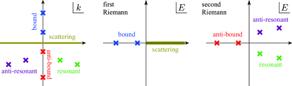
Figure 12: A schematic view of all possible eigenstates of the Schrödinger equation (55). See Table 1 for the precise attributes.

Table 1: All possible types of the eigenstates of the Schrödinger equation (55). By “continuum” eigenvalue, we mean a continuous spectrum, while by “discrete” eigenvalues, we mean point spectra. See Fig. 12 for a schematic view.

eigenfunction	eigenvalue	in the $k$ space		in the $E$ space	Riemann sheet
scattering state	continuum	real axis		positive real axis	first
bound state	discrete	positive imaginary axis		negative real axis	first
resonant state	discrete	the fourth quadrant		lower half plane	second
anti-resonant state	discrete	the third quadrant		upper half plane	second
anti-bound state	discrete	negative imaginary axis		negative real axis	second

The standard expansion of the unity and other quantities, such as Eq. (IV) (which is for the tight-binding model), uses all states in the first Riemann sheet but no states in the second. In contrast, the new expansion given in Refs. Hatano and Ordonez (2014); Tolstikhin et al. (1998); García-Calderón (2010); García-Calderón et al. (2012); Brown et al. (2016), such as Eq. (25) (which is again for the tight-binding model), uses all discrete states but no continuum states.

The scattering states are defined under the boundary condition

$$\psi(x)=\begin{cases}Ae^{ikx}+Be^{-ikx}&\quad\mbox{for $x<-L$},\\ Ce^{ikx}+De^{-ikx}&\quad\mbox{for $x>+L$},\end{cases}$$ (57)

with the flux conservation $|A|^{2}-|B|^{2}=|C|^{2}-|D|^{2}$, because of which the wave number $k$ is real and the eigenvalue given by Eq. (56) is real positive. All discrete states, on the other hand, are defined under the Siegert boundary condition Gamow (1928); Siegert (1939); Peierls (1959); le Couteur (1960); Zel’dovich (1960); Hokkyo (1965); Romo (1968); Berggren (1970); Gyarmati and Vertse (1971); Landau and Lifshitz (1977); Romo (1980); Berggren (1982, 1996); de la Madrid et al. (2005); Hatano et al. (2008); García-Calderón (2010):

$$\psi(x)\sim e^{ik|x|}\quad\mbox{for $|x|>L$}.$$ (58)

This definition is indeed equivalent to the textbook definition of the resonant states as the poles of the S matrix Hatano (2013). It includes a bound state as the case in which $k$ is a pure imaginary number with the positive imaginary part.

The other discrete states, namely the resonant, anti-resonant, and anti-bound states, all have negative imaginary part, and hence their eigenfunctions diverge in the limit $|x|\to\infty$. Because of this divergence, these states are often called unphysical and perhaps viewed skeptically, but it has been proved Hatano et al. (2008, 2009) that the resonant states maintain the probability interpretation; by incorporating the time-dependent part as in

$$\Psi(x,t)=\psi(x)e^{-iEt},$$ (59)

we indeed realize that the spatial divergence is canceled out by the temporal decay due to the negative imaginary part of the energy eigenvalue. From the point of view of the Landauer formula Landauer (1957); Datta (1995), the spatial divergence indicates the situation that the particle baths at the ends of the semi-infinite leads contain macroscopic numbers of the particles while the quantum scatterer in the middle contains only a microscopic number.

Appendix B Derivation of the expression (15) of the resonant-state component of the survival amplitude

In this appendix we derive Eq. (15). The matrix elements of the eigenstates of the Hamiltonian appearing in Eq. (IV) are given by Sasada et al. (2011)

$$\langle d_{1}|\phi_{k\alpha}\rangle =\langle d_{1}|\frac{1}{E_{k}-H+i0}H_{1}|{k_{\alpha}}\rangle$$

$$=-\sqrt{2}t_{2\alpha}\sin(k)\langle d_{1}|\frac{1}{E_{k}-H+i0}|d_{2}\rangle$$ (60)

for $-\pi<k\leq\pi$, where the matrix element of the Green’s function is

$$\langle d_{1}|\frac{1}{E_{k}-H+i0}|d_{2}\rangle$$

$$=\frac{-g}{(E_{k}-\varepsilon_{d_{1}})(E_{k}-\varepsilon_{d_{2}}+e^{ik}\sum_{\alpha}t_{2\alpha}^{2}/b)-g^{2}}.$$ (61)

Equation (B) is then expressed in terms of $\lambda=e^{ik}$ as

$$\langle d_{1}|\phi_{k\alpha}\rangle=\frac{-igt_{2\alpha}}{\sqrt{2}}\frac{\lambda-\frac{1}{\lambda}}{f(\lambda)}$$ (62)

with $f(\lambda)$ given in Eq. (IV). Its absolute value squared is

$$\left|\langle d_{1}|\phi_{k\alpha}\rangle\right|^{2} =\frac{g^{2}t_{2\alpha}^{2}}{2}\left|\frac{\lambda-\lambda^{-1}}{f(\lambda)}\right|^{2}$$

$$=\frac{g^{2}t_{2\alpha}^{2}}{2}\frac{\left(\lambda-\frac{1}{\lambda}\right)^{2}}{f(\lambda^{-1})-f(\lambda)}\left(\frac{1}{f(\lambda)}-\frac{1}{f(\lambda^{-1})}\right)$$ (63)

because $\lambda^{\ast}=\lambda^{-1}$ for real $k$, and hence $f(\lambda)^{\ast}=f(\lambda^{-1})$. In this expression, $f(\lambda^{-1})-f(\lambda)$ simplifies to

$$f(\lambda^{-1})-f(\lambda)=-h(\lambda)\sum_{\alpha}\frac{t_{2\alpha}^{2}}{b}\left(\lambda-\frac{1}{\lambda}\right),$$ (64)

where $h(\lambda)=h(\lambda^{-1})$ is given in Eq. (17). The survival amplitude in Eq. (IV) then takes the form

$$A(t)=\sum_{n\in\mbox{\scriptsize bound}}\langle d_{1}|\phi_{n}\rangle e^{-iE_{n}t}\langle\phi_{n}|d_{1}\rangle$$

$$-\frac{1}{2\pi i}\int_{O}\frac{d\lambda}{\lambda}\left(\lambda-\frac{1}{\lambda}\right)\exp\left[ib\left(\lambda+\frac{1}{\lambda}\right)t\right]$$

$$\times\frac{bg^{2}}{2h(\lambda)}\left[\frac{1}{f(\lambda)}-\frac{1}{f(\lambda^{-1})}\right],$$ (65)

where the integration contour $O$ is the counterclockwise unit circle on the $\lambda$ complex plane. Changing variables from $\lambda$ to $\lambda^{-1}$ for the term with $f(\lambda^{-1})$, we have

$$A(t)=\sum_{n\in\mbox{\scriptsize bound}}\langle d_{1}|\phi_{n}\rangle e^{-iE_{n}t}\langle\phi_{n}|d_{1}\rangle$$

$$-\int_{O}\frac{d\lambda}{2\pi i\lambda}\left(\lambda-\frac{1}{\lambda}\right)\exp\left[ib\left(\lambda+\frac{1}{\lambda}\right)t\right]\frac{bg^{2}}{h(\lambda)}\frac{1}{f(\lambda)}.$$ (66)

The function $f(\lambda)$ in Eq. (IV) can be written as

$$f(\lambda)=\frac{b^{2}}{\lambda^{2}}P_{4}(\lambda),$$ (67)

where $P_{4}(\lambda)$ is a fourth-order polynomial,

$$P_{4}(\lambda)=\prod_{n=1}^{4}(\lambda-\lambda_{n}),$$ (68)

which has four roots $\lambda_{n}$ corresponding to two bound-state eigenvalues and a resonant-antiresonant pair of complex-conjugate eigenvalues of the Hamiltonian, for the parameters of Fig. 6.

The bound-state terms in Eq. (B) are residues of the integral over $\lambda$ at the bound-state eigenvalues, so that they can be included in the integral over $\lambda$ by adding counterclockwise integrations around these eigenvalues. This gives the final result in Eq. (15).

Appendix C Proof of expression (25) of the survival amplitude

In Eq. (B), the function $h(\lambda)$ in Eq. (17) is proportional to a second-order polynomial as

$$h(\lambda)=-\frac{b}{\lambda}(\lambda-\lambda_{0})(\lambda-\lambda_{0}^{-1}),$$ (69)

where

$$\lambda_{0}=\frac{1}{2}\left(-\frac{\varepsilon_{1}}{b}+\sqrt{\frac{{\varepsilon_{1}}^{2}}{b^{2}}-4}\right).$$ (70)

Using a partial-fraction expansion we have

$$\frac{1}{h(\lambda)f(\lambda)}=\frac{\lambda^{3}}{b^{3}(\lambda-\lambda_{0})(\lambda-\lambda_{0}^{-1})\prod_{n=1}^{4}(\lambda-\lambda_{n})}$$

$$=\sum_{n=1}^{4}\frac{W_{n}}{\lambda-\lambda_{n}}+\frac{W_{0}}{\lambda-\lambda_{0}}+\frac{W_{\bar{0}}}{\lambda-\lambda_{0}^{-1}},$$ (71)

where the coefficients are given by

$$W_{n} =\lim_{\lambda\to\lambda_{n}}\frac{\lambda-\lambda_{n}}{h(\lambda_{n})f(\lambda)},$$ (72)

$$W_{0} =\lim_{\lambda\to\lambda_{0}}\frac{\lambda-\lambda_{0}}{h(\lambda)f(\lambda_{0})}=\frac{\lambda_{0}}{b}\frac{1}{\lambda_{0}-\lambda_{0}^{-1}}\frac{1}{f(\lambda_{0})},$$ (73)

$$W_{\bar{0}} =\lim_{\lambda\to\lambda_{0}^{-1}}\frac{\lambda-\lambda_{0}^{-1}}{h(\lambda)f(\lambda_{0}^{-1})}=\frac{\lambda_{0}^{-1}}{b}\frac{1}{\lambda_{0}^{-1}-\lambda_{0}}\frac{1}{f(\lambda_{0}^{-1})}$$

$$=-\lambda_{0}^{-2}W_{0},$$ (74)

and in the last line we used

$$f(\lambda_{0}^{-1})=f(\lambda_{0}),$$ (75)

which follows from the fact that when $h(\lambda)=0$, i.e., when $\lambda=\lambda_{0}$ or $\lambda=\lambda_{0}^{-1}$, we have $f(\lambda)=f(\lambda^{-1})=-g^{2}$ in Eq. (IV).

In Eq. (B) we can write

$$\frac{1}{h(\lambda)}\left[\frac{1}{f(\lambda)}-\frac{1}{f(\lambda^{-1})}\right]=\frac{1}{h(\lambda)f(\lambda)}-\frac{1}{h(\lambda^{-1})f(\lambda^{-1})}$$ (76)

since $h(\lambda)=h(\lambda^{-1})$. Introducing the partial-fraction expansion, Eq. (C), into Eq. (76) we have

$$\frac{1}{h(\lambda)f(\lambda)}-\frac{1}{h(\lambda^{-1})f(\lambda^{-1})}=\sum_{n=1}^{4}\left(\frac{W_{n}}{\lambda-\lambda_{n}}-\frac{W_{n}}{\lambda^{-1}-\lambda_{n}}\right)$$

$$+\frac{W_{0}}{\lambda-\lambda_{0}}+\frac{W_{\bar{0}}}{\lambda-\lambda_{0}^{-1}}-\frac{W_{0}}{\lambda^{-1}-\lambda_{0}}-\frac{W_{\bar{0}}}{\lambda^{-1}-\lambda_{0}^{-1}}.$$ (77)

The second line in Eq. (C) can be shown to vanish identically for $W_{\bar{0}}=-\lambda_{0}^{-2}W_{0}$. Hence, the terms involving $W_{0}$ and $W_{\bar{0}}$ cancel, and Eq. (B) reduces to

$$A(t)=\sum_{n\in\mbox{\scriptsize bound}}\langle d_{1}|\phi_{n}\rangle e^{-iE_{n}t}\langle\phi_{n}|d_{1}\rangle$$

$$-\frac{1}{2\pi i}\int_{O}\frac{d\lambda}{\lambda}\left(\lambda-\frac{1}{\lambda}\right)\exp\left[ib\left(\lambda+\frac{1}{\lambda}\right)t\right]$$

$$\times\frac{bg^{2}}{2}\left[\sum_{n=1}^{4}\frac{W_{n}}{\lambda-\lambda_{n}}-\sum_{n=1}^{4}\frac{W_{n}}{\lambda^{-1}-\lambda_{n}}\right].$$ (78)

We remark that the poles of $h(\lambda)$ do not contribute to the integral.

Changing the integration variable from $\lambda$ to $\lambda^{-1}$ for the last term we get

$$A(t)=\sum_{n\in\mbox{\scriptsize bound}}\langle d_{1}|\phi_{n}\rangle e^{-iE_{n}t}\langle\phi_{n}|d_{1}\rangle$$

$$-\int_{O}\frac{d\lambda}{2\pi i}\left(\lambda-\frac{1}{\lambda}\right)\exp\left[ib\left(\lambda+\frac{1}{\lambda}\right)t\right]$$

$$\times\frac{bg^{2}}{\lambda}\sum_{n=1}^{4}\frac{W_{n}}{\lambda-\lambda_{n}}.$$ (79)

Expressing the bound-state terms as residues around the poles $\lambda_{n}$ with $n\in\rm{bound}$ we obtain

$$A(t)=\int_{C}\frac{d\lambda}{2\pi i}\left(\lambda-\frac{1}{\lambda}\right)\exp\left[ib\left(\lambda+\frac{1}{\lambda}\right)t\right]$$

$$\times\frac{bg^{2}}{\lambda}\sum_{n=1}^{4}\frac{W_{n}}{\lambda-\lambda_{n}},$$ (80)

where $C$ is the contour of Fig. 3. A further partial-fraction expansion gives

$$\frac{1}{\lambda}\frac{W_{n}}{\lambda-\lambda_{n}}=\frac{W_{n}}{\lambda_{n}}\left(\frac{1}{\lambda-\lambda_{n}}-\frac{1}{\lambda}\right).$$ (81)

The isolated term $-1/\lambda$ gives a vanishing integral because

$$\int_{C}\frac{d\lambda}{2\pi i}\frac{1}{\lambda}\left(\lambda-\frac{1}{\lambda}\right)\exp\left[ib\left(\lambda+\frac{1}{\lambda}\right)t\right]$$

$$=\int_{C}\frac{d\lambda}{2\pi i}\frac{1}{ibt}\frac{\partial}{\partial\lambda}\exp\left[ib\left(\lambda+\frac{1}{\lambda}\right)t\right]=0.$$ (82)

Therefore

$$A(t)=\int_{C}\frac{d\lambda}{2\pi i}\left(\lambda-\frac{1}{\lambda}\right)\exp\left[ib\left(\lambda+\frac{1}{\lambda}\right)t\right]$$

$$\times bg^{2}\sum_{n=1}^{4}\frac{W_{n}}{\lambda_{n}}\frac{1}{\lambda-\lambda_{n}}.$$ (83)

For $t=0$, the residue of Eq. (C) at $\lambda=\lambda_{n}$ is the same as the residue of the Green’s function at the pole $E_{n}$,

$$R_{n}\equiv\int_{C_{n}}\frac{dz}{2\pi i}\frac{1}{z-H}={\rm Res}\left[\frac{1}{z-H}\right]_{z=E_{n}},$$ (84)

where $C_{n}$ is a small contour surrounding the pole $E_{n}$ in a counterclockwise direction. In the following we will prove that $R_{n}=\Phi_{n}$, where $\Phi_{n}=|\phi_{n}\rangle\langle{\tilde{\phi}}_{n}|$ is a dyad of discrete eigenstates of the Hamiltonian.

Since $H\Phi_{n}=\Phi_{n}H=E_{n}\Phi_{n}$, we can show by taking matrix elements that

$$\langle j|\Phi_{n}|l\rangle=\sum_{k\neq l}\frac{1}{E_{n}-\varepsilon_{j}}\langle j|H_{1}|k\rangle\langle k|\Phi_{n}|l\rangle,$$ (85)

where $\varepsilon_{j}=\langle j|H_{0}|j\rangle$. On the other hand, the Green’s function obeys the relation

$$\frac{1}{z-H}=\frac{1}{z-H_{0}}+\frac{1}{z-H_{0}}H_{1}\frac{1}{z-H},$$ (86)

which leads to

$$\langle j|R_{n}|l\rangle=\sum_{k\neq l}\frac{1}{E_{n}-\varepsilon_{j}}\langle j|H_{1}|k\rangle\langle k|R_{n}|l\rangle.$$ (87)

Therefore $R_{n}$ and $\Phi_{n}$ obey exactly the same equation. Moreover, we have that $\Phi_{n}\Phi_{n^{\prime}}=\delta_{nn^{\prime}}\Phi_{n}$ and $R_{n}\Phi_{n^{\prime}}=\delta_{nn^{\prime}}\Phi_{n}$, which shows that $R_{n}$ and $\Phi_{n}$ have the same normalization. Therefore, we conclude that $R_{n}=\Phi_{n}$.

By identifying the residue of Eq. (C) at $\lambda=\lambda_{n}$ with $R_{n}$ (and therefore with $\Phi_{n}$) for $t=0$, we arrive to

$$-\left(\lambda_{n}-\frac{1}{\lambda_{n}}\right)bg^{2}\frac{W_{n}}{\lambda_{n}}=\langle d_{1}|\phi_{n}\rangle\langle{\tilde{\phi}}_{n}|d_{1}\rangle,$$ (88)

which leads to

$$A(t)=\int_{C}\frac{d\lambda}{2\pi i}\left(\lambda-\frac{1}{\lambda}\right)\exp\left[ib\left(\lambda+\frac{1}{\lambda}\right)t\right]$$

$$\times\sum_{n=1}^{4}\frac{\langle d_{1}|\phi_{n}\rangle\langle{\tilde{\phi}}_{n}|d_{1}\rangle}{\lambda_{n}^{-1}-\lambda_{n}}\frac{1}{\lambda-\lambda_{n}}.$$ (89)

Finally, using Eq. (27) we have

$$\frac{\langle d_{1}|\phi_{n}\rangle\langle{\tilde{\phi}}_{n}|d_{1}\rangle}{\lambda_{n}^{-1}-\lambda_{n}} =\lambda_{n}\frac{\langle d_{1}|\phi_{n}\rangle\langle{\tilde{\phi}}_{n}|d_{1}\rangle}{1-\lambda_{n}^{2}}$$

$$=\lambda_{n}\langle d_{1}|\psi_{n}\rangle\langle{\tilde{\psi}}_{n}|d_{1}\rangle,$$ (90)

which gives Eq. (25).

Appendix D Derivation of the expression (VIII) of the survival amplitude

We will express the survival amplitude in terms of an integral of a Bessel function Garmon and Ordonez (2017). The final result is given in Eq. (VIII).

We start by separating the survival amplitude in Eq. (25) into two terms: one, $A_{C}(t)$, due to the clockwise contour around the unit circle in Fig. 3, and the other, $A_{B}(t)$, due to the small contours around the bound-state eigenvalues. The survival amplitude is then $A(t)=A_{C}(t)+A_{B}(t)$.

Hereafter we consider the $A_{C}(t)$ term. Changing variables from $\lambda$ to $k$ (with $\lambda=e^{ik}$) we have

$$A_{C}(t)=\frac{1}{2\pi i}\sum_{n=1}^{2N}\int_{\pi}^{-\pi}dk(ie^{ik})(-2i\sin k)e^{2itb\cos k}$$

$$\times\langle d_{1}|\psi_{n}\rangle\frac{\lambda_{n}}{e^{ik}-\lambda_{n}}\langle\tilde{\psi}_{n}|d_{1}\rangle.$$ (91)

Multiplying and dividing the integrand by $(e^{-ik}-\lambda_{n})$ and exchanging the integration limits we obtain

$$A_{C}(t)=\frac{-1}{2\pi i}\sum_{n=1}^{2N}\int_{-\pi}^{\pi}dk(2\sin k)e^{2itb\cos k}$$

$$\times\langle d_{1}|\psi_{n}\rangle\frac{b(1-e^{ik}\lambda_{n})}{-2b\cos k-E_{n}}\langle\tilde{\psi}_{n}|d_{1}\rangle.$$ (92)

Hereafter we will assume that $E_{n}$ is a resonant eigenvalue, and hence has a negative imaginary part. If it is a bound-state eigenvalue, for which the imaginary part is zero, we can add an infinitesimal imaginary part $-i\epsilon$ to $E_{n}$ and then take the limit $\epsilon\to 0$ at the end. If $E_{n}$ is an anti-resonant eigenvalue, which has a positive imaginary part, then the integration over $\tau$ in Eq. (D) below should be done from $0$ to $-\infty$.

Assuming $\operatorname{\mathrm{Im}}E_{n}<0$ we have

$$A_{C}(t)=\frac{-b}{2\pi i}\sum_{n=1}^{2N}\int_{-\pi}^{\pi}dk(2\sin k)e^{2itb\cos k}$$

$$\times(-i)\int_{0}^{\infty}d\tau e^{-i\tau(2b\cos k+E_{n})}\langle d_{1}|\psi_{n}\rangle(1-e^{ik}\lambda_{n})\langle\tilde{\psi}_{n}|d_{1}\rangle.$$ (93)

Terms that are even in $k$ in the second line of Eq. (D) give a vanishing integral. Hence we have

$$A_{C}(t)=\sum_{n=1}^{2N}\frac{b\lambda_{n}}{\pi i}\int_{0}^{\infty}d\tau e^{-i\tau E_{n}}\int_{-\pi}^{\pi}dk\,\sin^{2}k\,e^{2i(t-\tau)b\cos k}$$

$$\times\langle d_{1}|\psi_{n}\rangle\langle\tilde{\psi}_{n}|d_{1}\rangle.$$ (94)

The integral over $k$ can be written in terms of the Bessel function $J_{1}$:

$$\int_{-\pi}^{\pi}dk\,\sin^{2}k\,e^{2i(t-\tau)b\cos k}=\pi\frac{J_{1}[2b(t-\tau)]}{b(t-\tau)}.$$ (95)

This gives

$$A_{C}(t)=\sum_{n=1}^{2N}(-i)\lambda_{n}\langle d_{1}|\psi_{n}\rangle\langle\tilde{\psi}_{n}|d_{1}\rangle I(E_{n},t),$$ (96)

where

$$I(E_{n},t)=\int_{0}^{\infty}d\tau e^{-i\tau E_{n}}\frac{J_{1}[2b(t-\tau)]}{t-\tau}.$$ (97)

Now we change the integration variable $\tau$ to $t^{\prime}=t-\tau$:

$$I(E_{n},t) =\int_{-\infty}^{t}dt^{\prime}e^{-iE_{n}(t-t^{\prime})}\frac{J_{1}(2bt^{\prime})}{t^{\prime}}$$

$$=e^{-iE_{n}t}\left(\int_{-\infty}^{0}dt^{\prime}+\int_{0}^{t}dt^{\prime}\right)e^{iE_{n}t^{\prime}}\frac{J_{1}(2bt^{\prime})}{t^{\prime}}.$$ (98)

The integral from $-\infty$ to $0$ can be evaluated exactly in terms of the hypergeometric function ${}_{2}F_{1}$ http://dlmf.nist.gov/13. (10):

$$\int_{-\infty}^{0}dt^{\prime} e^{iE_{n}t^{\prime}}\frac{J_{1}(2bt^{\prime})}{t^{\prime}}$$

$$=\int_{0}^{\infty}dt^{\prime}e^{-iE_{n}t^{\prime}}\frac{J_{1}(2bt^{\prime})}{t^{\prime}}$$

$$=\frac{b}{iE_{n}}\frac{\Gamma(1)}{\Gamma(2)}{}_{2}F_{1}\left(\frac{1}{2},1;2;\frac{4b^{2}}{E_{n}^{2}}\right)$$

$$=\frac{b}{iE_{n}}\left(\frac{1}{2}+\frac{1}{2}\sqrt{1-\frac{4b^{2}}{E_{n}^{2}}}\right)^{-1}$$

$$=i\lambda_{n}^{s},$$ (99)

where $s=1$ if $|\lambda_{n}|<1$ (bound states) and $s=-1$ otherwise. Therefore we obtain

$$I(E_{n},t)=ie^{-iE_{n}t}\left[\lambda_{n}^{s}-i\int_{0}^{t}dt^{\prime}\,e^{iE_{n}t^{\prime}}\frac{J_{1}(2bt^{\prime})}{t^{\prime}}\right]$$ (100)

and

$$A_{C}(t)=\sum_{n=1}^{2N}\lambda_{n}\langle d_{1}|\psi_{n}\rangle\langle\tilde{\psi}_{n}|d_{1}\rangle$$

$$\times e^{-iE_{n}t}\left[\lambda_{n}^{s}-i\int_{0}^{t}dt^{\prime}\,e^{iE_{n}t^{\prime}}\frac{J_{1}(2bt^{\prime})}{t^{\prime}}\right].$$ (101)

Note that for the resonant state we do not need to include the contribution $A_{B}(t)$. We then obtain Eq. (VIII).

Appendix E Derivation of the expression (VIII) of the resonant-state component of the survival amplitude

In this Appendix we derive Eq. (VIII) that gives the resonant-state component of the survival amplitude. We start with Eq. (VIII), which can be expressed as

$$A_{{\rm R}}(t)=\langle d_{1}|\psi_{R}\rangle\langle\tilde{\psi}_{R}|d_{1}\rangle$$

$$\times e^{-iE_{R}t}\left[1-i\lambda_{R}\left(\int_{0}^{\infty}-\int_{t}^{\infty}\right)dt^{\prime}\,e^{iE_{R}t^{\prime}}\frac{J_{1}(2bt^{\prime})}{t^{\prime}}\right].$$ (102)

By analytic continuation of Eq. (D), the integral from $0$ to $\infty$ can be shown to be

$$\int_{0}^{\infty}dt^{\prime}\,e^{iE_{R}t^{\prime}}\frac{J_{1}(2bt^{\prime})}{t^{\prime}}=-i\lambda_{R}.$$ (103)

Therefore we have

$$A_{{\rm R}}(t)=\langle d_{1}|\psi_{R}\rangle\langle\tilde{\psi}_{R}|d_{1}\rangle$$

$$\times e^{-iE_{R}t}\left[1-\lambda_{R}^{2}+i\lambda_{R}\int_{t}^{\infty}dt^{\prime}\,e^{iE_{R}t^{\prime}}\frac{J_{1}(2bt^{\prime})}{t^{\prime}}\right].$$ (104)

For the states $|\phi_{R}\rangle=\sqrt{1-\lambda_{R}^{2}}|\psi_{R}\rangle$ and $\langle{\tilde{\phi}}_{R}|=\sqrt{1-\lambda_{R}^{2}}\langle{\tilde{\psi}}_{R}|$, Eq. (VIII) follows.

Up to this point we have considered positive $t$. In Appendix F we will need to consider negative $t$. For a negative time $-t$, the first line of Eq. (D) gives

$$I(E_{n},-t) =\int_{-\infty}^{-t}dt^{\prime}e^{-iE_{n}(-t-t^{\prime})}\frac{J_{1}(2bt^{\prime})}{t^{\prime}}$$

$$=\int_{t}^{\infty}dt^{\prime}e^{iE_{n}(t-t^{\prime})}\frac{J_{1}(2bt^{\prime})}{t^{\prime}},$$ (105)

where we changed integration variable from $t^{\prime}$ to $-t^{\prime}$ and used $J_{1}(-x)=-J_{1}(x)$. This gives

$$A_{{\rm R}}(-t)=\langle d_{1}|\psi_{R}\rangle\langle\tilde{\psi}_{R}|d_{1}\rangle$$

$$\times e^{iE_{R}t}(-i\lambda_{R})\int_{t}^{\infty}dt^{\prime}\,e^{-iE_{R}t^{\prime}}\frac{J_{1}(2bt^{\prime})}{t^{\prime}}.$$ (106)

Appendix F Long-time approximation of the resonant-state component and estimation of $r(t)$ for large $t$

For large $t$ we neglect the purely exponential term in Eq. (E) to obtain

$$A_{{\rm R}}(t)=i\lambda_{R}\langle d_{1}|\psi_{R}\rangle\langle\tilde{\psi}_{R}|d_{1}\rangle e^{-iE_{R}t}\int_{t}^{\infty}dt^{\prime}\,e^{iE_{R}t^{\prime}}\frac{J_{1}(2bt^{\prime})}{t^{\prime}}.$$ (107)

For $t^{\prime}\gtrsim 1$ the Bessel function is approximated as

$$J_{1}(2bt^{\prime})\approx\sqrt{\frac{1}{\pi bt^{\prime}}}\sin\left(2bt^{\prime}-\pi/4\right).$$ (108)

The integral in Eq. (107) can then be expressed in terms of the incomplete Gamma function,

$$\int_{t}^{\infty}dt^{\prime}\,e^{iE_{R}t^{\prime}}\frac{J_{1}(2bt^{\prime})}{t^{\prime}}\approx\frac{i\lambda_{R}}{2i\sqrt{\pi}}$$

$$\times\left[e^{-i\pi/4}\left(\frac{ib}{2b+E_{R}}\right)^{-1/2}\Gamma\left(-\frac{1}{2},-it(2b+E_{R})\right)\right.$$

$$\left.-e^{i\pi/4}\left(\frac{ib}{-2b+E_{R}}\right)^{-1/2}\Gamma\left(-\frac{1}{2},-it(-2b+E_{R})\right)\right],$$ (109)

where

$$\Gamma(a,z)=\int_{z}^{\infty}\tau^{a-1}e^{-\tau}d\tau.$$ (110)

For large $z$ the incomplete Gamma function is approximately given by

$$\Gamma(a,z)\approx z^{a-1}e^{-z}.$$ (111)

Using this approximation for large $t\gg 1/|E_{R}\pm 2b|$ in Eq. (F), we obtain

$$A_{{\rm R}}(t)=i\lambda_{R}\langle d_{1}|\psi_{R}\rangle\langle\tilde{\psi}_{R}|d_{1}\rangle\frac{1}{2\sqrt{\pi}}(bt)^{-3/2}$$

$$\times\left[\left(\frac{be^{-i\pi/4}}{2b+E_{R}}\right)e^{2ibt}+\left(\frac{be^{i\pi/4}}{2b-E_{R}}\right)e^{-2ibt}\right],$$ (112)

which gives the power law decay of the survival probability in the form $t^{-3}$ Khalfin (1957); Garmon et al. (2013); Hatano and Ordonez (2014); Garmon and Ordonez (2017).

Similarly from Eq. (E) we obtain for large negative time

$$A_{{\rm R}}(-t) = -i\lambda_{R}\langle d_{1}|\psi_{R}\rangle\langle\tilde{\psi}_{R}|d_{1}\rangle\frac{1}{2\sqrt{\pi}}(bt)^{-3/2}$$ (113)

$$\times \left[\left(\frac{be^{-i\pi/4}}{2b-E_{R}}\right)e^{2ibt}+\left(\frac{be^{i\pi/4}}{2b+E_{R}}\right)e^{-2ibt}\right].$$

For long times, the ratio of the resonance component of the survival amplitude to the anti-resonant component is

$$r(t) =\left|\frac{A_{R}(t)}{A_{R}(-t)}\right|$$

$$=\left|\frac{\left(\frac{e^{-i\pi/4}}{2b+E_{R}}\right)e^{2ibt}+\left(\frac{e^{i\pi/4}}{2b-E_{R}}\right)e^{-2ibt}}{\left(\frac{e^{-i\pi/4}}{2b-E_{R}}\right)e^{2ibt}+\left(\frac{e^{i\pi/4}}{2b+E_{R}}\right)e^{-2ibt}}\right|.$$ (114)

If the imaginary part of $E_{R}$ is much smaller than its real part (e.g. the Fermi golden rule is applicable), then the ratio is close to $1$.

Appendix G Derivation of the Green’s function for the Friedrichs model

In this appendix we obtain the Green’s function in Eq. (48). For the Friedrichs model, the Green’s function is given by Petrosky et al. (1991)

$$G^{\pm}(E)\equiv\langle 1|\frac{1}{E-H\pm i0}|1\rangle=\frac{1}{\eta^{\pm}(E)},$$ (115)

where

$$\eta^{\pm}(E) \equiv E-\omega_{1}-\sum_{k}\frac{V_{k}^{2}}{E^{\pm}-\omega_{k}}$$ (116)

and $E^{\pm}=E\pm i0$. In the continuous limit the summation approaches an integral as

$$\eta^{\pm}(E) =E-\omega_{1}-g^{2}\int_{-\infty}^{\infty}dk\frac{\sqrt{\beta\omega_{k}}}{\omega_{k}+\beta}\frac{1}{E^{\pm}-\omega_{k}}$$

$$=E-\omega_{1}-2g^{2}\int_{0}^{\infty}dk\frac{\sqrt{\beta k}}{k+\beta}\frac{1}{E^{\pm}-k}.$$ (117)

In the second line we used $\omega_{k}=|k|$. We can integrate it over $k$ explicitly by changing the integration variable from $k$ to $u=\sqrt{k}$, which gives

$$\int_{0}^{\infty}dk\frac{\sqrt{\beta k}}{k+\beta}\frac{1}{E^{\pm}-k}$$

$$=-2\sqrt{\beta}\int_{0}^{\infty}du\frac{u^{2}}{u^{2}+\beta}\frac{1}{u^{2}-E^{\pm}}$$

$$=-2\frac{\sqrt{\beta}}{\beta+E^{\pm}}\int_{0}^{\infty}du\left(\frac{\beta}{u^{2}+\beta}+\frac{E^{\pm}}{u^{2}-E^{\pm}}\right)$$

$$=\frac{-2\sqrt{\beta}}{\beta+E^{\pm}}\left[\sqrt{\beta}\arctan\frac{u}{\sqrt{\beta}}+\frac{\sqrt{E^{\pm}}}{2}\ln\left(\frac{u+\sqrt{E^{\pm}}}{u-\sqrt{E^{\pm}}}\right)\right]_{0}^{\infty}$$

$$=\frac{-\pi}{\beta+E^{\pm}}\left(\beta+i\sqrt{\beta E^{\pm}}\right)=\frac{-\pi}{\beta+E^{\pm}}\left(\beta\pm i\sqrt{\beta E}\right).$$ (118)

In the last line we used the fact that the branch cut of the square root is along the positive $E$ axis. Inserting this result into Eq. (G), we obtain the Green’s function in Eq. (48).