Holographic Complexity for Time-Dependent Backgrounds

Davood Momeni^a,∗, Mir Faizal^b,c,‡, Sebastian Bahamonde^d,†, Ratbay Myrzakulov^a

^aEurasian International Center for Theoretical Physics and Department of General Theoretical Physics, Eurasian National University, Astana 010008, Kazakhstan
^b Irving K. Barber School of Arts and Sciences, University of British Columbia - Okanagan, 3333 University Way, Kelowna, British Columbia V1V 1V7, Canada
^cDepartment of Physics and Astronomy, University of Lethbridge, Lethbridge, Alberta, T1K 3M4, Canada.
^dDepartment of Mathematics,University College London, Gower Street, London, WC1E 6BT, UK

E-mails : ^∗davoodmomeni78@gmail.com,^‡mirfaizalmir@googlemail.com,^†sebastian.beltran.14@ucl.ac.uk

In this paper, we will analyse the holographic complexity for time-dependent asymptotically $AdS$ geometries. We will first use a covariant zero mean curvature slicing of the time-dependent bulk geometries, and then use this co-dimension one spacelike slice of the bulk spacetime to define a co-dimension two minimal surface. The time-dependent holographic complexity will be defined using the volume enclosed by this minimal surface. This time-dependent holographic complexity will reduce to the usual holographic complexity for static geometries. We will analyse the time-dependence as a perturbation of the asymptotically $AdS$ geometries. Thus, we will obtain time-dependent asymptotically $AdS$ geometries, and we will calculate the holographic complexity for such a time-dependent geometries.

1 Introduction

An observation made from different branches of physics is that the physical laws can be represented by informational theoretical processes [1, 2]. The information theory deals with the ability of an observer to process relevant information, it is important to know how much information is lost during a process, and this is quantified by entropy. As the laws of physics are represented by informational theoretical processes, entropy is a very important physical quantity, and so it has been used from condensed matter physics to gravitational physics. In fact, in the Jacobson formalism, the geometry of spacetime can also be obtained from the scaling behavior of the maximum entropy of a region of space [3, 4]. This scaling behavior of maximum entropy of a region of space is obtained from the physics of black holes. As black holes are maximum entropy objects, and this maximum entropy of a black hole scales with its area, it can be argued that the maximum entropy of a region of space scales with the area of its boundary. This scaling behavior has led to the development of the holographic principle [5, 6], which states that the degrees of freedom in a region of space is equal to the degrees of freedom on the boundary of that region. The $AdS/CFT$ correspondence is a concrete realizations of the holographic principle [7], and it relates the string theory in the bulk of an $AdS$ spacetime to the superconformal field theory on its boundary.

It is interesting to note that the holographic principle which was initially motivated from the physics of black holes, has in turn been used to propose a solution to the black hole information paradox [8, 9]. This is because it has been proposed that the black hole information paradox might get solved by analyzing the of microstates of a black hole, and the quantum entanglement of a black hole can be used to study such microstates. This quantum entanglement is quantified using the holographic entanglement entropy, and $AdS/CFT$ correspondence can be used to calculate the holographic entanglement entropy. The holographic entanglement entropy of a conformal field theory on the boundary of an asymptotically $AdS$ spacetime is dual to the area of a minimal surface in the bulk of an asymptotically $AdS$ spacetime. Thus, for a subsystem $A$ (with its complement), it is possible to define $\gamma_{A}$ as the $(d-1)$-minimal surface extended into the bulk of the $AdS$ spacetime, such that its boundary is $\partial A$. This minimal surface is obtained by first foliating the bulk spacetime by constant time slices, and then defining a minimal surface on such a slice of the bulk spacetime. The holographic entanglement entropy can be calculated using the area of this minimal surface [10, 11]

$${S}_{A}=\frac{Area(\gamma_{A})}{4G_{d+1}}\,,$$ (1.1)

where $G$ is the gravitational constant for the $AdS$ spacetime. This minimal surface is a co-dimension two surface in the bulk spacetime because of being a co-dimension one submanifold of a particular leaf of the spacelike foliation. It is possible to generalize the holographic entanglement entropy to time-dependent geometries [26]. This is because even thought it is not possible to foliate a bulk time-dependent geometry by a preferred time slicing, it is possible to foliation a time-dependent asymptotically $AdS$ geometry by zero mean curvature slicing. Thus, it is possible to take slices of the bulk geometry with vanishing trace of extrinsic curvature. This corresponds to taking the spacelike slices with maximal area through the bulk, anchored at the boundary. This covariant foliation reduces to the constant time foliation for static geometries. Thus, a co-dimension one spacelike foliation of time-dependent asymptotically $AdS$ geometry can be performed, and on such a spacelike slice the metric is spacelike, and so a co-dimension two minimal surface can be defined on such a spacelike slice. So, in this formalism, first a maximal spacelike slice of the bulk geometry is obtained though the mean curvature slicing, and then a minimal surface $\gamma_{At}$ is constructed on this spacelike slice [26]. This minimal surface reduces to the usual minimal surface for static geometries, and so for static geometries, $\gamma_{At}=\gamma_{A}$, as the mean curvature slicing reduces to the constant time slicing for such geometries. This minimal area surface $\gamma_{At}$ can be used to define the time-dependent holographic entanglement entropy for a time-dependent geometry [26],

$${S}_{A}=\frac{Area(\gamma_{At})}{4G_{d+1}}\,.$$ (1.2)

It may be noted that for the static case this time-dependent holographic entanglement entropy reduces to the usual definition of holographic entanglement entropy, so for the static case, we have ${S}_{A}(\gamma_{At})={S}_{A}(\gamma_{A})$.

The entropy measures how much information is lost in a system. However, it is also important to know how easy is for an observer to obtain the information present in a system. This difficulty to obtain information from a system is quantified by a new quantity called complexity, just as the loss of information is quantified by entropy. Furthermore, as physical laws can be represented by information theoretical processes, complexity is expected to become another fundamental physical quantity describing the laws of physics. In fact, complexity has already been used to study condensed matter systems [12, 13], molecular physics [14], and quantum computing [15]. It is also expected that complexity might be used to solve the black hole information paradox, as the recent studies seem to indicate that the information may not be actually lost in a black hole, but it would be effectively lost, as it would be impossible to reconstruct it from the Hawking radiation [16]. However, unlike entropy, there is no universal definition of complexity of a system, and there are different proposals for defining the complexity of a system. It is possible to define the complexity of a boundary theory, as a quantity which is holographically dual to a volume of co-dimension one time slice in an anti-de Sitter (AdS) spacetime [17, 18, 19, 20]. In fact, it is possible to used the volume $V(\gamma_{A})$ enclosed by the minimal surface $\gamma_{A}$ to define holographic complexity [21]. This is the same minimal surface which was used to calculated the holographic entanglement entropy. Thus, we can write the holographic complexity as [21]

$$\mathcal{C}_{A}=\frac{V(\gamma_{A})}{8\pi RG_{d+1}},$$ (1.3)

where $R$ and $V$ are the radius of the curvature and the volume in the $AdS$ spacetime, respectively. It may be noted that there are other ways to define the volume in bulk $AdS$, and these correspond to other proposals for the complexity of the boundary theory [22]. It has been possible to use an alternative proposal for holographically analyse quantum phase transitions [23, 24, 25]. However, we shall not use such proposals in this paper, and we will only concentrate on the proposal where the holographic complexity is dual to the volume enclosed by the minimal surface used to calculate the holographic entanglement entropy [21].

As we will be analyzing time-dependent geometries in this paper, we need to generalize holographic complexity to time-dependent holographic complexity. It may be noted the holographic entanglement entropy has been generalized to a time-dependent holographic entanglement entropy using a covariant formalism [26]. Motivated by this definition of time-dependent holographic entanglement entropy [26], we will use the same covariant formalism to define the time-dependent holographic complexity for time-dependent geometries. Thus, we will first foliate the time-dependent asymptotically $AdS$ geometry by zero mean curvature slicing, and so each of these slices of the bulk geometry will have vanishing trace of extrinsic curvature. This will corresponds to taking the spacelike slices with maximal area through the bulk, anchored at the boundary. Thus, we will get a co-dimension one surface with a spacelike metric, and we will again define a co-dimension two minimal surface $\gamma_{At}$ on this spacelike slice of the bulk geometry. It will be the same minimal surface which was used to calculate the time-dependent holographic entanglement entropy [26]. However, now we will calculate the volume enclosed by this minimal surface $V(\gamma_{At})$, and use this volume to define the time-dependent holographic complexity as

$$\mathcal{C}_{A}=\frac{V(\gamma_{At})}{8\pi RG_{d+1}},$$ (1.4)

where $\mathcal{C}_{A}$ is the time-dependent holographic complexity. It may be noted that this surface $\gamma_{At}$ reduces to the usual minimal surface $\gamma_{A}$ for the static geometries, so the volume enclosed by this surface will also reduce to the volume enclosed by the usual minimal surface for static geometries. Thus, this time-dependent holographic complexity will also reduce to the usual definition of holographic complexity for static geometries, and so for static geometries, we have $\mathcal{C}_{A}(\gamma_{At})=\mathcal{C}_{A}(\gamma_{A})$. It may be noted that non-equilibrium field theory has been used for analyzing various aspects of the holography using $AdS/CFT$ correspondence, and such study is relevant for holographically analysing the time-dependent geometries [27, 28, 30, 31, 32]. Furthermore, time-evolution of holographic entanglement entropy has been studied using the metric perturbations [36]. This was done by analyzing the time-dependence as a perturbation of a background geometry. A time-dependent background induced by quantum quench was analysed using the continuum version of the multi-scale entanglement renormalization [33]. The causal wedges associated with a given sub-region in the boundary of a time-dependent asymptotically $AdS$ geometry have been used for understanding causal holographic information [34]. This was done by using a Vaidya-$AdS$ geometry for analysing the behavior a null dust collapse in an asymptotically $AdS$ spacetime. In this analysis, the behavior of holographic entanglement entropy was also discussed. Holographic complexity, just like holographic entanglement entropy, is a important physical quantity which can be calculated holographically. Therefore, we have generalize holographic complexity to time-dependent holographic complexity, and now we can use it for analysing time-dependent geometries. So, in this paper, we will analyse the time-dependent holographic complexity for such time-dependent geometries.

2 Time-Dependent Geometry

In this section, we will analyse a time-dependent asymptotically $AdS$ geometry by analysing time-dependent perturbation of a pure $AdS$ geometry. We will also study the behavior of the time-dependent holographic complexity for such a geometry. This time-dependent geometry can be modeled using the Vaidya spacetime, and the metric for this spacetime can be written as

$$ds^{2}=\frac{1}{z^{2}}\Big{[}-F(t,z)dt^{2}-2dtdz+H(t,z)dx^{2}\Big{]}\,,$$ (2.1)

where $F(t,z)$ and $H(t,z)$ are functions of the ingoing Eddington-Finkelstein time coordinate $t$, and $z$ is the radial Poincare direction. For the specific case where $z=0$, we recover the $AdS$ boundary. It is not possible to define a temperature for a time-dependent backgrounds as this geometry does not have a time Killing vector. However, it has been demonstrated that the time-dependence can be analysed as a perturbation around this static geometry, and this was done for analysing the time-dependence of holographic entanglement entropy [35, 36]. So, we will also analyse the the time-dependence of this metric as a perturbation around a static geometry, and use it for analyzing the time-dependence of holographic complexity. Now if we we neglect the time-dependence of this geometry, by defining a static geometry with $F(z)=F(z,t)|_{t=0}$, then for this static geometry, the standard Hawking-Bekenstein horizon temperature $T$ can be obtained by choosing the event horizon as the smallest root of the equation $F(z)=0$. We will assume that we have a strip geometry such that its width is $2L$ in the $x$ direction. Now because of the symmetries of the surface, $t=t(x)$ and $z=z(x)$ are only functions of $x$, and the surface $\gamma_{A}$ will be characterized by the embedding

$$\gamma_{A}=\{t=t(x),z=z(x)\}\,.$$ (2.2)

Now for a extremal surface which extends smoothly into the bulk, we can assume that the center of the strip is located at $x=0$. This surface is smooth, and it satisfies the following the boundary conditions

$$t(x=0) = t^{*}\,,$$

$$z(x=0) = z^{*}\,,$$ (2.3)

$$t^{\prime}(x=0) = z^{\prime}(x=0)=0\,,$$

where prime denotes differentiation with respect to $x$. These boundary conditions define the turning point of the strip at $x=0$. It is important to note that the time $t$ in the metric (2.1) refers to the ingoing time in the Eddington-Finkelstein coordinates. Since we are located at the boundary, the physical time is $T=t+z$ (near $z\to 0$). Furthermore, at $x=L$, we need to deal with the following UV boundary conditions,

$$t(x=L)=T-\epsilon\,,\ \ z(x=L)=\epsilon\,.$$ (2.4)

where $\epsilon\sim 0$ is a cut-off introduced to deal with the UV divergence at the boundary $z=0$. Now, we can express the area of the minimal surface $\gamma_{A}$ as

$$\textrm{Area}(\gamma_{A})=\int_{-L}^{L}\frac{dx\,H(t(x),z(x))}{z(x)^{2}}\sqrt{H(t(x),z(x))^{2}-F(t(x),z(x))t^{\prime 2}-2t^{\prime}(x)z^{\prime}(x)}\,,$$ (2.5)

where $t=t(x)$ and $z=z(x)$, and so the functions $H(t,z)$ and $F(t,z)$ only depend on $x$. It may be noted that the Lagrangian density in the integrand has a conserved charge. The area can be now expressed as

$$\textrm{Area}(\gamma_{A})=\int_{-L}^{L}dx\Big{(}\frac{H^{2}}{z^{2}}\frac{z^{*}}{H^{*}}\Big{)}^{2}\,,$$ (2.6)

where $H^{*}=H(t^{*},z^{*})$ is a constant. Finally, the time-dependent holographic complexity for the metric (2.1), can be written as

$$\mathcal{C}_{A}(T)=\lim_{\epsilon\to 0}\frac{V(\gamma_{A})}{8\pi RG_{3}}\,,$$ (2.7)

where the co-dimension one volume $V(\gamma_{A})$, can be expressed as

$$V(\gamma_{A})=\int_{T-\epsilon}^{t^{*}}\frac{dt}{t^{\prime}(t)}\frac{tz^{\prime}(x(t))}{z(x(t))}\,.$$ (2.8)

The quantity (2.7) is the time-dependent extension of the usual holographic complexity, which can be used for analyzing this time-dependent geometry.

The holographic complexity for a pure $AdS_{3}$ spacetime can be obtained by integrating (2.7),

$$\mathcal{C}_{A}(T)=\frac{1}{8\pi RG_{3}}\Big{[}t^{*}-T+(t^{*}+z^{*})\log\Big{(}\frac{z^{*}}{t^{*}+z^{*}-T}\Big{)}\Big{]}\,.$$ (2.9)

We will use numerical analysis to study the behavior of this quantity. To do that we will fix the strip size to be

$$2L=\int_{\epsilon}^{z^{*}}\frac{dz}{z^{\prime}(z)}\,,$$ (2.10)

and then we can find the minimal surface at each $z^{*}$. We will also assume $z^{*}\approx 3.39L$. Using the Euler-Lagrange equations, we can directly obtain $z^{\prime}(z)=\sqrt{\big{(}z^{*}/z\big{)}^{4}-1}$. Fig. 1 shows the behavior of the regularized holographic complexity $\mathcal{C}_{A}(T)$ as a function of the time coordinate $T=t+z$, for different values of $t^{*}$. It can be observed that this has a minima at $T=0$.

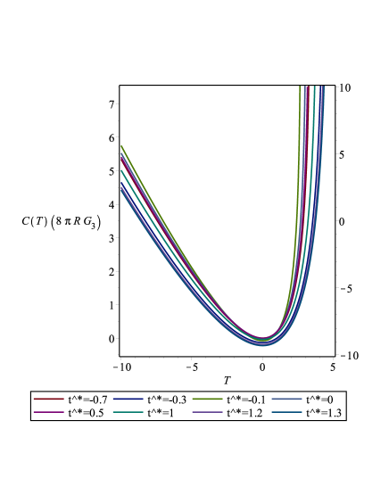
Figure 1: Regularized holographic complexity for pure $AdS_{3}$ v.s time coordinate $T$. We used different values for $t^{*}$. The schematic graph predicts a minima at $T=0$. The system at early time has the minimum for holographic complexity.

Now from (2.9) and the Fig.1, we can observe that the holographic complexity becomes small near $T\approx 0$. In fact, near this point, the holographic complexity has a minimum. We observe that by increasing the value of $t^{*}$, the dip becomes deeper and steeper, for $L=1$. Thus, the system will remain close to the $AdS$ boundary $z=0$ if $T=t^{*}$. In this limit, we observe that the system evolves to a equilibrium state with $\mathcal{C}_{A}(T)=0$. Furthermore, at late times, the tip point $z^{*}$, will also meet the horizon.

3 Metric Perturbations

In this section, we will use metric perturbation to analyse to calculate holographic complexity for time-dependent geometries. It may be noted that time-dependent asymptotically $AdS$ geometries are interesting, and have been used for analyzing various different systems. In fact, it is expected that using the $AdS/CFT$ correspondence these background will be dual to interesting field theory solutions, and these field theory solutions can represent interesting physical systems. In fact, it has been demonstrated that supergravity solution on a time-dependent orbifold background is dual to a noncommutative field theory with time-dependent noncommutative parameter [37]. The time-dependent noncommutativity can have lot of interesting applications for modeling nonlinear phenomena in quantum optics [38]. Thus, it is interesting to analyse such backgrounds. Furthermore, we will analyse the holographic complexity for such backgrounds, and this can be used to obtain the complexity for the boundary theory. Complexity being an important physical quantity in condensed matter systems [12, 13] and molecular physics [14], it would be interesting to obtain it for condensed matter systems dual to such time-dependent backgrounds. However, a problem with this approach is that the absence of a time Killing vector in such geometries makes it difficult to perform such an analysis. So, in this section, we will use a perturbative technique, which has been used for analysing the holographic entanglement entropy of time-dependent $AdS$ geometries [36], for analyzing the holographic complexity of time-dependent $AdS$ geometry. The holographic entanglement entropy has been calculated using a perturbative technique for a small deformations of a $AdS$ vacuum spacetime [36]. Thus, a background $AdS$ spacetime can used for this analysis, and on this background spacetime small time-dependent perturbation can analysed. The use of perturbative technique makes it possible to calculate different physical quantities on this background. Thus, using the same formalism as has been used for analyzing the time-dependent holographic entanglement entropy for a time-dependent background, we will now analyse the time-dependent holographic complexity for such a background. Now for an $AdS_{d+1}$ spacetime with radius $\ell$, the metric can be written as

$$ds^{2}=\frac{\ell^{2}}{\cos^{2}x}\Big{[}-dt^{2}+dx^{2}+\sin^{2}x(d\theta^{2}+\sin^{2}\theta d\Omega_{d-2}^{2})\Big{]}\,,$$ (3.1)

where the metric for the unit-sphere is denoted by $d\Omega_{d-2}^{2}$. Here we have split the $S^{d-1}$ metric into a polar angle $\theta$ and a unit-radius sphere $S^{d-2}$.

Now, we will assume that an entangling region on the boundary is a cap-like one defined between $0\leq\theta<\theta_{0}$, and we will use the boundary time $t=t_{0}$. The extremized area, which can be used to obtain the holographic complexity, is given by the following functional of $x(\theta)$,

$$\textrm{Area}=\ell^{d-1}\text{vol}(S^{d-2})\int^{\theta_{0}}_{0}d\theta\frac{(\sin x\sin\theta)^{d-2}}{\cos^{d-1}x}\sqrt{\left(\frac{dx}{d\theta}\right)^{2}+\sin^{2}x}\,\,.$$ (3.2)

Now if we assume that $\theta_{0}<\pi/2$, then the holographic complexity can be written as

$$\mathcal{C}_{A}=\frac{\ell^{d-1}\text{vol}(S^{d-2})}{8\pi G}\int^{\theta_{0}}_{0}d\theta(\sin\theta)^{d-2}\int_{0}^{x(\theta)}dx\frac{(\sin x)^{d-1}}{\cos^{d}x}\,\,.$$ (3.3)

It is important to mention that it is difficult to find the most general exact solution for $x(\theta)$ derived from the action (3.2). However, we can use an appropriate solution which satisfies the Euler-Lagrange equations in any dimension $d$, and we will use this solution to analyse metric perturbations. Further, we will assume that at the boundary, this solution satisfies $x=\pi/2$, and it is mapped to $a=\cos\theta_{0}$. We will call this solution as the constant-latitude solution, and it will be explicitly written as

$$x(\theta)=\sin^{-1}\left(\frac{a}{\cos\theta}\right)\,.$$ (3.4)

For this solution, from (3.3), we obtain

$$\mathcal{C}_{A}=\frac{\ell^{d-1}\text{vol}(S^{d-2})}{8\pi G(d-1)}\int^{\theta_{0}}_{0}d\theta(\sin\theta)^{d-2}\big{(}1-\frac{a^{2}}{\cos^{2}\theta}\big{)}^{1-d}F\Big{(}\frac{1-n}{2},1-\frac{n}{2},\frac{3-n}{2},1-\frac{a^{2}}{\cos^{2}\theta}\Big{)}\,.$$ (3.5)

Now we can investigate small deformations of an $AdS$ background and then analyse the corrections to the minimal area solution (3.4) from those small deformations. These corrections will produce correction terms for the volume enclosed by this minimal surface, and this will in turn produce correction terms for the holographic complexity. We can parametrize the coordinates $\theta$ and $x$ as

$$z=\cos\theta,\quad\rho=\sin x\,.$$ (3.6)

Now the area functional can be written as

$$\text{Area}=\ell^{d-1}\text{vol}(S^{d-2})\int^{1}_{\cos^{-1}\theta_{0}}dz\frac{\rho^{d-2}(1-z^{2})^{(d-2)/2}}{(1-\rho^{2})^{d/2}}\sqrt{(\rho^{\prime})^{2}+\frac{\rho^{2}(1-\rho^{2})}{1-z^{2}}}\,.$$ (3.7)

Furthermore, using this parametrization, the holographic complexity can be expressed as

$$\mathcal{C}_{A}=\frac{\ell^{d-1}\text{vol}(S^{d-2})}{8\pi G(d-1)}\int_{\cos^{-1}\theta_{0}}^{1}dz(1-z^{2})^{\frac{d-3}{2}}\big{(}1-\frac{a^{2}}{z^{2}}\big{)}^{1-d}F\Big{(}\frac{1-n}{2},1-\frac{n}{2},\frac{3-n}{2},1-\frac{a^{2}}{z^{2}}\Big{)}\,.$$ (3.8)

In order to calculate the holographic complexity, we need to substitute the solution $\rho=a/z$ back into (3.8), and then perform the integral. As is common in $AdS/CFT$ correspondence, this integral is divergent near the $AdS$ boundary, $x=\pi/2$. So, we introduce the following cut-off

$$x_{m}=\pi/2-\epsilon\,.$$ (3.9)

Now by mapping the original solution (3.4), we obtain

$$\theta_{m}=\theta_{0}-\frac{1}{2}\epsilon^{2}\cot\theta_{0},\quad\text{i.e.}\quad z_{m}=a\left(1+\frac{\epsilon^{2}}{2}\right)\,.$$ (3.10)

It is well-known that excited states in conformal field theory tare dual to deformations of the $AdS$ spacetime. So, it is interesting to analyze small metric perturbations around an $AdS$ spacetime. These small deformation can be used to obtain the holographic complexity for excited states of the dual conformal field theory. As we want to analyse the time-geometries, we will analyse the time-dependent deformations. As this spacetimes will also be spherically symmetric, we can write the metric for this spacetime as

$$ds^{2}=\frac{\ell^{2}}{\cos^{2}x}\biggl{(}-A(t,x)e^{-2\delta(t,x)}dt^{2}+A^{-1}(t,x)dx^{2}+\sin^{2}x(d\theta^{2}+\sin^{2}\theta d\Omega^{2}_{d-2})\biggr{)}\,,$$ (3.11)

where the pure $AdS$ metric is recovered by choosing $A=1$ and $\delta=0$. In terms of new variables $\rho=\sin x,z=\cos\theta$, and $\rho=\rho(z)$ and $t=t(z)$, the area functional (3.7) can be expressed as

$$\frac{\text{Area}}{\text{vol}(S^{d-2})}=\int dz\frac{\rho^{d-2}(1-z^{2})^{\frac{d-3}{2}}}{(1-\rho^{2})^{\frac{d-1}{2}}}\sqrt{-g_{tt}(1-z^{2})(t^{\prime})^{2}+\frac{g_{xx}(1-z^{2})}{1-\rho^{2}}(\rho^{\prime})^{2}+\rho^{2}}\,,$$ (3.12)

where primes denote differentiation with respect to $z$, and

$$g_{tt} = Ae^{-2\delta}=1-2\sum_{n=1}^{\infty}\nu_{n}(t,\rho)\epsilon^{n}\,,$$ (3.13)

$$g_{xx} = A^{-1}=1+2\sum_{n=1}^{\infty}m_{n}(t,\rho)\epsilon^{n}\,.$$ (3.14)

Here, we have also defined a dimensionless perturbation parameter $\epsilon$. Now from Eq. (3.11), we obtain that the holographic complexity for such a time-dependent geometry as,

$$\mathcal{C}_{A}=\frac{\text{vol}(S^{d-2})l^{d-1}}{8\pi G}\int d\rho\frac{\rho^{d-1}}{\sqrt{1-\rho^{2}}}\int dz\frac{A^{-1/2}(t(z),\rho)z^{d-2}}{\sqrt{1-z^{2}}}\,.$$ (3.15)

We can also use a perturbative approach to compute the minimal-area surface. We know that for the pure $AdS$ spacetime, the solutions are $\rho(z)=a/z,t(z)=t_{0}$, and so, we can assume that the perturbative solutions will statisfy

$$\rho(z) = \frac{a}{z}+\sum_{n=1}^{\infty}\rho_{n}(z)\epsilon^{n}\,,$$ (3.16)

$$t(z) = t_{0}+\sum_{n=1}^{\infty}t_{n}(z)\epsilon^{n}\,,$$ (3.17)

where we have expanded the solutions in term of the small parameter $\epsilon$. So, we can analyse such solutions using this perturbative technique. We can thus obtain time-dependent holographic complexity for different time-dependent geometries.

4 Deformation

In this section, we will analyse the time-dependent holographic complexity for deformations of $AdS$ spacetime. It may be noted that various deformation of the $AdS$ spacetime are dual to interesting physical systems. It has been demonstrated that a Schwarzschild black hole in an $AdS$ background can be used to analyse high spin baryon in hot strongly coupled plasma. This is because such a system can be analysed using the finite-temperature supersymmetric Yang-Mills theory, and this theory is dual to the Schwarzschild black hole in a $AdS$ background [39]. So, it would be interesting to analyse such deformations of a time-dependent $AdS$ background, as this can be used to obtain the complexity of the field theory dual to such backgrounds. It may be noted that such a deformation of a time-dependent $AdS$ spacetime has been used to obtain the conformal field theory dual to a FLRW background [40]. It would be interesting to analyse the holographic complexity for such systems, as this is an important physical quantity. So, in this section, we analyse a simple examples of a deformation $AdS$ spacetimes, and then we evaluate the integral (3.15) using perturbative techniques. Thus, we will find the first order corrections to the minimal surfaces $\rho_{1}(z),t_{1}(z)$, and then use it to obtain the corrections to holographic complexity. Now we can analyse a geometry with a small mass, which is a minimal deformation of the pure $AdS$ spacetime. The mass terms deforms this geometry to a light Schwarzschild-$AdS$ spacetime. Thus, we will use this time-dependent formalism for analysing the time-dependent Schwarzschild black hole in $AdS$ background. The horizon, which is located at $r=h$, satisfies $f_{d}(h)=0$, and so we can define the following perturbative parameter,

$$\epsilon\equiv M\ell^{2}/h^{d}\ll 1\,.$$ (4.1)

The area expressed in terms of $t(\theta)$ and $r(\theta)$, can be written as

$$\text{Area}=\text{vol}(S^{d-2})\int_{0}^{r_{0}}dr(r\sin\theta(r))^{d-2}\sqrt{\frac{1}{f}-ft^{\prime 2}+r^{2}\theta(r)^{\prime 2}}\,,$$ (4.2)

where prime denotes differentiation with respect to $r$ , and the extremal surfaces are defined by $t(r)$ and $\theta(r)$. The holographic complexity in usual coordinates can be written as

$$\mathcal{C}_{A}=\frac{\text{vol}(S^{d-2})t_{0}}{d}\int_{0}^{\theta_{0}}r(\theta)^{d}(\sin\theta)^{d-2}d\theta\,.$$ (4.3)

In order to evaluate the integral, we have to obtain the solution to the Euler-Lagrange equation for $\theta(r)$. As we want to apply this formalism to a specific example, so we will now apply it to $AdS_{3}$ to simplify calculations. The $AdS_{3}$ spacetime has been used to analyse various interesting physical systems. The holographic duals to time-like warped $AdS_{3}$ spacetimes have been studied, and it was demonstrated that such systems have at least one Virasoro algebra with computable central charge [41]. In fact, it was also observed that there exists a dense set of points in the moduli space of these models in which there is also a second commuting Virasoro algebra. The higher spin theories on an $AdS_{3}$ background have been studied [42]. The field theory dual to such a background has also been analysed, and constraints on the central charge of such a field theory dual have been obtained from the modular invariance. It may be noted that time-dependent solution for D-branes have been analysed using $AdS_{3}$ spacetime [43]. In this work, D-branes solutions where analysed using a $\kappa$-deformed background with non-trivial dilaton and Ramond-Ramond fields. So, it is interesting to analyse the time-dependent deformation of $AdS_{3}$ spacetime. The $AdS_{3}$ spacetime has also been used to analyse the microstates of black holes [44]. Thus, $AdS_{3}$ spacetime has been used for analyzing interesting physical systems, and it would be interesting to analyse the deformation of $AdS_{3}$ spacetime. So, we will apply this formalism to $AdS_{3}$ spacetime, and the equation for $\theta(r)$ for this spacetime can be written as (4.2). Now for this spacetime geometry, we obtain

$$\frac{r^{2}\theta^{\prime}(r)}{\sqrt{\frac{1}{f}-ft^{\prime 2}+r^{2}\theta(r)^{\prime 2}}}=p,\ \ \frac{-ft^{\prime}}{\sqrt{\frac{1}{f}-ft^{\prime 2}+r^{2}\theta(r)^{\prime 2}}}=E.$$ (4.4)

As this metric is static, we can write $g_{ta}=0$ and $\partial g_{\mu\nu}/\partial t=0$. Thus, the equation for $t(z)$ at leading order gives us a trivial solution $t^{0}(z)=t_{0}$, and the equations for $t(r)$ and $\theta(r)$ can be written as

$${\frac{d}{dr}}t\left(r\right) = \displaystyle{\frac{{\ell}^{3}Er\left(\epsilon\,{h}^{2}{p}^{2}-{h}^{2}\epsilon\,{r}^{2}+{\ell}^{2}{r}^{4}-{\ell}^{2}{p}^{2}+{r}^{2}{\ell}^{2}-{r}^{2}{\ell}^{2}{p}^{2}+{E}^{2}{\ell}^{2}{r}^{2}\right)^{-1/2}}{-{\ell}^{2}-{r}^{2}{\ell}^{2}+\epsilon\,{h}^{2}}}\,,$$ (4.5)

$${\frac{d}{dr}}\theta\left(r\right) = \displaystyle{\frac{p\left(\epsilon\,{h}^{2}{p}^{2}-{h}^{2}\epsilon\,{r}^{2}+{\ell}^{2}{r}^{4}-{\ell}^{2}{p}^{2}+{r}^{2}{\ell}^{2}-{r}^{2}{\ell}^{2}{p}^{2}+{E}^{2}{\ell}^{2}{r}^{2}\right)^{-1/2}}{r}}\,.$$ (4.6)

We can expand $f$ in series of $\epsilon$ as $f=(1+r^{2}/\ell^{2})-\epsilon\,r_{+}^{2}/\ell^{2}$. Using this expansion, we can solve the above equation for $t(r)=t_{0}+\,t^{1}(r)$ and $\theta(r)=\theta^{0}(r)+\epsilon\,\theta^{1}(r)$. Thus, up to first order in $\epsilon$, we obtain

$$t^{1}(r)=\frac{1}{2\ell^{2}}\,\left(-E{h}^{2}\int\!{\frac{3\,{r}^{5}+\left(3-3\,{p}^{2}+2\,{E}^{2}\right){r}^{3}-3\,r{p}^{2}}{\left({r}^{4}+\left(1-{p}^{2}+{E}^{2}\right){r}^{2}-{p}^{2}\right)^{3/2}\left(1+{r}^{2}\right)^{2}}}{dr}+2\,{C_{1}}\,{\ell}^{2}\right)\,,$$ (4.7)

$$\theta^{1}(r)=-\frac{1}{2\ell^{3}}\,\left(p{h}^{2}\int\!{\frac{{p}^{2}-{r}^{2}}{r\left({r}^{2}-{r}^{2}{p}^{2}+{r}^{4}-{p}^{2}+{E}^{2}{r}^{2}\right)^{3/2}}}{dr}-2\,{C_{2}}\,{\ell}^{3}\right)\,.$$ (4.8)

Finally, using this solution, we obtain the holographic complexity for this geometry,

$$\Delta\mathcal{C}=\mathcal{C}_{SAdS_{3}}-\mathcal{C}_{AdS_{3}}\approx\frac{t_{0}}{2}\frac{M\ell^{2}}{h^{2}}\int_{0}^{\theta_{0}}r^{2}\partial_{r}\theta^{1}(r)dr.$$ (4.9)

The first order correction for the holographic complexity of the $AdS_{3}$ background can be written as

$$\Delta\mathcal{C} = \frac{t_{0}}{4}\frac{M\ell^{2}}{h^{2}}\,Im\Big{[}\Big{(}\left(2\,{p}^{2}+1+2\,{E}^{2}+{p}^{4}-2\,{p}^{2}{E}^{2}+{E}^{4}\right){\ell}^{3}\Xi\Big{)}^{-1}\times$$ (4.10)

$$\Big{(}p{h}^{2}\left(i{p}^{2}{E}^{2}-i{p}^{2}-i{p}^{4}+i{p}^{2}{r_{{0}}}^{2}+i{r_{{0}}}^{2}+i{E}^{2}{r_{{0}}}^{2}+p\Xi+{p}^{3}\Xi-p\Xi\,{E}^{2}\right)\Big{)}\Big{]}\,,$$

where we have introduced the parameter $\Xi=\sqrt{{r_{{0}}}^{4}+{r_{{0}}}^{2}-{p}^{2}{r_{{0}}}^{2}+{E}^{2}{r_{{0}}}^{2}-{p}^{2}}$ and $Im(z)$ denotes the imaginary part of $z$.

After we have demonstrated how this formalism can be used to analyse perturbations, we will apply it for analysing a time-dependent metric. So, we will find the holographic complexity for a time-dependent deformation of the $AdS_{3}$, given by the metric (3.11). Thus, using the time-dependent formalism [36], we now analyze the spectrum of a massive scalar field in the background (3.11). The scalar field with conformal mass $m^{2}=\Delta(\Delta-d)/\ell^{2}$ can be described by the following equation,

$$\partial_{t}(e^{\delta}A^{-1}\partial_{t}\phi)-\frac{1}{\tan^{d-1}x}\partial_{x}(Ae^{-\delta}\tan^{d-1}x\partial_{x}\phi)+\frac{\Delta(\Delta-d)}{\cos^{2}x}e^{-\delta}\phi=0\,.$$ (4.11)

The Einstein’s field equations reduced to the first order system of differential equations for this scalar field $\phi$,

$$\delta^{\prime} = -\sin x\cos x(A^{-2}e^{2\delta}\dot{\phi}^{2}+\phi^{\prime 2})\,,$$ (4.12)

$$A^{\prime} = A\delta^{\prime}+\frac{d-2+2\sin^{2}x}{\sin x\cos x}(1-A)-\frac{\Delta(\Delta-d)\sin x}{\cos x}\phi^{2}\,.$$ (4.13)

We can now use a perturbative technique to find solutions for this system. Thus, we will use a small deformations of the metric in the $AdS_{3}$ spacetime. So, we will use the following time-dependent background,

$$\delta(t,u) = \epsilon\left[-1+u^{8}+\frac{3\cos(8t)}{5}+u^{8}\cos(8t)-\frac{8u^{10}\cos(8t)}{5}\right]\,,$$ (4.14)

$$A(t,u) = 1-\epsilon\left[\frac{2u^{4}}{3}+\frac{2u^{6}}{3}-\frac{4u^{8}}{3}-2u^{8}\cos(8t)+2u^{10}\cos(8t)\right]\,.$$ (4.15)

where $u=\cos x=\sqrt{1-\rho^{2}}$. We have to use a first order perturbation regime for these metric functions, and the perturbed functions, $t(z)$ and $\rho(z)$. These solutions are given by [36],

$$\rho_{1}(z) = \frac{a(a^{2}-z^{2})^{2}(36z^{4}-a^{2}z^{2}(33+25z^{2})+2a^{4}(5+3z^{2}+3z^{4}))}{105z^{9}}$$ (4.16)

$$+\frac{a(a^{2}-z^{2})^{2}}{315z^{11}}\biggl{(}-82z^{6}+a^{2}z^{4}(151+95z^{2})-2a^{4}z^{2}(60+31z^{2}+32z^{4})$$

$$+a^{6}(35+15z^{2}+16z^{4}+16z^{6})\biggr{)}\cos(8t_{0})\,,$$

$$t_{1}(z) = -\frac{(a^{2}-z^{2})^{2}}{315z^{10}}\biggl{(}-19z^{6}+19a^{2}z^{4}(-2+5z^{2})+a^{4}(69z^{2}-62z^{4}-64z^{6})$$ (4.17)

$$+a^{6}(-28+15z^{2}+16z^{4}+16z^{6})\biggr{)}\sin(8t_{0})\,.$$

So, for $d=2$, we can evaluate (3.15), up to first order in $\epsilon$,

$$\mathcal{C}_{A}=\frac{\ell}{8\pi G}\int d\rho\frac{\rho}{\sqrt{1-\rho^{2}}}\int dz\frac{A^{-1/2}(t(z),\rho)}{\sqrt{1-z^{2}}}\,.$$ (4.18)

Finally, by perturbing $\delta(t,u)$ and $A(t,u)$ for $t(z)=t_{0}+\epsilon\,t_{1}(z)$ and $\rho(z)=a/z+\epsilon\,\rho_{1}(z)$, we obtain, the following expression for holographic complexity

$$\Delta\mathcal{C}=\frac{\ell}{24\pi G}\int_{\eta}^{1}{\frac{\Pi(z)}{{z}^{11}\sqrt{{z}^{2}-{a}^{2}}\sqrt{1-{z}^{2}}}}\,,$$ (4.19)

where

$$\Pi(z) = -3\,{z}^{12}+3\,a{z}^{11}\rho_{{1}}\left(z\right)+11\,{a}^{4}{z}^{8}+3\,{z}^{10}{a}^{2}\cos\left(8\,t_{{0}}\right)-15\,{a}^{4}{z}^{8}\cos\left(8\,t_{{0}}\right)+30\,{a}^{6}{z}^{6}\cos\left(8\,t_{{0}}\right)$$ (4.20)

$$-15\,{a}^{6}{z}^{6}-30\,{a}^{8}{z}^{4}\cos\left(8\,t_{{0}}\right)+9\,{a}^{8}{z}^{4}+15\,{a}^{10}\cos\left(8\,t_{{0}}\right){z}^{2}-2\,{a}^{10}{z}^{2}$$

$$-3\,{a}^{12}\cos\left(8\,t_{{0}}\right)\,.$$

It may be noted that at the boundary $z=a$, we have to introduce a cut-off $\eta$. Thus, Eq. (4.19) can be written as

$$\Delta\mathcal{C} = \frac{\ell}{24\pi G}\sum_{m=0}^{\infty}\left(\left(2\,m\right)!\,{4}^{-m}\sum_{k=0}^{\infty}{\frac{\left({a}^{-2}\right)^{k}\left(2\,k\right)!\,{4}^{-k}{z}^{2\,k}}{\sqrt{-{a}^{2}}\left(k!\right)^{2}}}\left(m!\right)^{-2}\right)\times$$ (4.21)

$$\Big{[}B_{mk}\left(1\right)-B_{mk}\left(\eta\to 0\right)\Big{]}\,,$$

where $\rho_{1}(z)$ is given by (4.16), and we have defined

$$B_{mk}(z) = \int dz\,{z}^{2\,m-11+2\,k}(-3\,{z}^{12}+3\,a{z}^{11}\rho_{{1}}\left(z\right)+11\,{a}^{4}{z}^{8}+3\,{z}^{10}{a}^{2}\cos\left(8\,t_{{0}}\right)-15\,{a}^{4}{z}^{8}\cos\left(8\,t_{{0}}\right))$$ (4.22)

$$+\int dz\,{z}^{2\,m-11+2\,k}(30\,{a}^{6}{z}^{6}\cos\left(8\,t_{{0}}\right)-15\,{a}^{6}{z}^{6}-30\,{a}^{8}{z}^{4}\cos\left(8\,t_{{0}}\right)+9\,{a}^{8}{z}^{4}$$

$$+15\,{a}^{10}\cos\left(8\,t_{{0}}\right){z}^{2})-\int dz\,{z}^{2\,m-11+2\,k}(2\,{a}^{10}{z}^{2}+3\,{a}^{12}\cos\left(8\,t_{{0}}\right))\,.$$

Thus, we are able to calculate the holographic complexity for a time-dependent background. This formalism can be used to obtain the complexity of the field theory dual to such a time-dependent background. Furthermore, it is also possible to use this formalism to analyse other time-dependent asymptotically $AdS$ geometries. So, we can use the results of this paper to analyse holographic complexity for various deformations of the $AdS$ geometries.

5 Conclusions

In this paper, we analyse the holographic complexity for time-dependent geometries. Just as the holographic entanglement entropy is dual to an area in the bulk of an $AdS$ spacetime, holographic complexity is as a quantity dual to a volume in the bulk $AdS$. In this paper, the concept of holographic complexity was generalized to a time-dependent holographic complexity. This time-dependent holographic complexity was defined as a quantity dual to volume of a region in a time-dependent $AdS$ geometry. Thus, we first foliated the time-dependent asymptotically $AdS$ geometry by zero mean curvature slicing, and obtained slices of the bulk geometry with vanishing trace of extrinsic curvature. This corresponded to taking the spacelike slices with maximal area through the bulk, anchored at the boundary. Thus, we obtained a co-dimension one surface with a spacelike metric. We used this co-dimension one surface to defined a co-dimension two minimal surface in the bulk geometry. It was be the same minimal surface which was used for calculating the time-dependent holographic entanglement entropy [26]. However, we calculating the volume enclosed by this minimal surface, and use this volume to define the time-dependent holographic complexity. It was observed that this definition of time-dependent holographic complexity reduced to the usual holographic complexity for static geometries. The metric perturbation has been used in this paper to analyse this behavior of time-dependent complexity. This has been motivated by the earlier works on the holographic entanglement entropy where such a perturbative technique was used for analysing the effects of small deformations of a $AdS$ spacetime. Thus, in this paper, the same technique was used for analysing holographic complexity for a small deformation of a $AdS$ spacetime. This formalism was finally applied for analyzing a time-dependent geometry. Thus, holographic complexity for a time-dependent background was studied in this paper.

It will be interesting to analyse other time-dependent backgrounds using the formalism developed in this paper. It may be noted that the string theory propagating in a pp-wave time-dependent background with a null singularity has been studied [45]. In this analysis, it has been demonstrated that entanglement entropy is dynamically generated by this background. It would be also interesting to analyse the holographic complexity for the string theory propagating in a pp-wave time-dependent background with a null singularity. Furthermore, the holographic entanglement entropy has been studied for various interesting systems, and it would be interesting to analyse the holographic complexity for such systems. The effects of deforming the renormalized entanglement entropy near the UV fixed point of a three dimensional field theory by a mass terms have been studied [46]. This analysis was performed using the Lin-Lunin-Maldacena geometries corresponding to the vacua of the mass-deformed ABJM theory. Thus, the small mass effect for various droplet configurations were analytically compute, and it was demonstrated that the renormalized entanglement entropy is monotonically decreasing at the UV fixed point. It would be interesting to calculate the holographic complexity for this system, and use it to analyse the behavior of this system.

References

- [1] K. H. Knuth , AIP Conf. Proc. 1305, 3 (2011)
- [2] P. Goyal, Information 3, 567 (2012)
- [3] T. Jacobson, Phys. Rev. Lett. 75, 1260 (1995)
- [4] R. G. Cai and S. P. Kim, JHEP 0502, 050 (2005)
- [5] G. ’t Hooft, [arXiv:gr-qc/9310026]
- [6] L. Susskind, J. Math. Phys. 36, 6377 (1995)
- [7] J. M. Maldacena, Adv. Theor. Math. Phys. 2, 231 (1998)
- [8] A. Strominger and C. Vafa, Phys. Lett. B 379, 99 (1996)
- [9] J. M. Maldacena, JHEP 0304, 021 (2003)
- [10] S. Ryu and T. Takayanagi, Phys. Rev. Lett. 96, 181602 (2006)
- [11] V. E. Hubeny, M. Rangamani and T. Takayanagi, JHEP 0707, 062 (2007)
- [12] F. Barahona, J. Phys. A 15, 3241 (1982)
- [13] M. Troyer and U. J. Wiese. Phys. Rev. Lett 94, 170201 (2005)
- [14] J. Grunenberg, Phys. Chem. Chem. Phys. 13, 10136 (2011)
- [15] M. Stanowski, Complicity 2, 78 (2011)
- [16] S. W. Hawking, M. J. Perry and A. Strominger, Phys. Rev. Lett. 116, 231301 (2016)
- [17] L. Susskind, Fortsch. Phys. 64, 24 (2016)
- [18] L. Susskind, Fortsch. Phys. 64, 24 (2016)
- [19] D. Stanford and L. Susskind, Phys. Rev. D 90, 12, 126007 (2014)
- [20] D. Momeni, S. A. H. Mansoori and R. Myrzakulov, Phys. Lett. B 756, 354 (2016)
- [21] M. Alishahiha, Phys. Rev. D 92, 126009 (2015)
- [22] M. Miyaji, T. Numasawa, N. Shiba,T. Takayanagi, and K. Watanabe, Phy. Rev. Lett 115, 261602 (2015)
- [23] H. T. Quan, Z. Song, X. F. Liu, P. Zanardi, and C. P. Sun, Decay of loschmidt echo enhanced by quantum criticality, Phys. Rev. Lett. 96, 140604 (2006)
- [24] P. Zanardi and N. Paunkoviic, Phys. Rev. E 74, 031123 (2006)
- [25] P. Zanardi, P. Giorda, and M. Cozzini, Phys. Rev. Lett. 99, 100603 (2007)
- [26] V. E. Hubeny, M. Rangamani and T. Takayanagi, JHEP 0707, 062 (2007)
- [27] P. M. Chesler, and L. G. Yaffe, Phys. Rev. Lett. 102, 211601 (2009)
- [28] K. Murata, S. Kinoshita and N. Tanahashi, JHEP 1007, 050 (2010)
- [29] S. R. Das, T. Nishioka and T. Takayanagi, JHEP 1007, 071 (2010)
- [30] M. Nozaki, T. Numasawa and T. Takayanagi, JHEP 1305, 080 (2013)
- [31] E. Caceres, A. Kundu, J. F. Pedraza and W. Tangarife, JHEP 1401, 084 (2014)
- [32] N. Bao, X. Dong, E. Silverstein and G. Torroba, JHEP 1110, 123 (2011)
- [33] M. Nozaki, S. Ryu and T. Takayanagi, JHEP 10, 193 (2012)
- [34] V. E. Hubeny, M. Rangamani and E. Tonni, JHEP 1305, 136 (2013)
- [35] X. Bai, B. H. Lee, L. Li, J. R. Sun and H. Q. Zhang, JHEP 1504, 066 (2015)
- [36] N. Kim and J. Hun Lee, J. Korean Phys. Soc. 69, 623 (2016)
- [37] M. Alishahiha and S. Parvizi, JHEP 0210, 047 (2002)
- [38] N. Chandra, J. Phys. A. Math. Theor. 45, 015307 (2012)
- [39] M. Li, Y. Zhou and S. Pu, JHEP 0810, 010 (2008)
- [40] N. Tetradis, JHEP 1003, 040 (2010)
- [41] S. Detournay, D. Israel, J. M. Lapan and M. Romo, JHEP 1101, 030 (2011)
- [42] A. Castro, A. Lepage-Jutier and A. Maloney, JHEP 1101, 142 (2011)
- [43] M. Khouchen and J. Kluson, JHEP 1508, 046 (2015)
- [44] M. Cvetic and F. Larsen, Phys. Rev. Lett. 82, 484 (1999)
- [45] A. L. Gadelha, D. Z. Marchioro and D. L. Nedel, Phys.Lett. B 639, 383 (2006)
- [46] K. K. Kim, O. K. Kwon, C. Park and H. Shin, Phys. Rev. D 90, 046006 (2014)