Argmin process The argmin process of random walks, Brownian motion and Lévy processes Jim Pitman and Wenpin Tang arcsine law; argmin process; Brownian extrema; Feller semigroup; Brownian excursion theory; jump process; Lévy process; Lévy system; Markov property; space-time shift process; path decomposition; random walks; renewal property; sample path property; stable process; stationary process. 60G50, 60G51, 60J65 August 22, 2017 June 6, 2018 23 2018 60 10.1214/18-EJP185 In this paper we investigate the argmin process of Brownian motion $B$ defined by $\alpha_{t}:=\sup\left\{s\in[0,1]:B_{t+s}=\inf_{u\in[0,1]}B_{t+u}\right\}$ for $t\geq 0$. The argmin process $\alpha$ is stationary, with invariant measure which is arcsine distributed. We prove that $(\alpha_{t};t\geq 0)$ is a Markov process with the Feller property, and provide its transition kernel $Q_{t}(x,\cdot)$ for $t>0$ and $x\in[0,1]$. Similar results for the argmin process of random walks and Lévy processes are derived. We also consider Brownian extrema of a given length. We prove that these extrema form a delayed renewal process with an explicit path construction. We also give a path decomposition for Brownian motion at these extrema.

1 Introduction and main results

In this paper we are interested in the argmin process $(\alpha_{t};t\geq 0)$ of standard Brownian motion $(B_{t};t\geq 0)$. That is,

$$\alpha_{t}:=\sup\left\{s\in[0,1]:B_{t+s}=\inf_{u\in[0,1]}B_{t+u}\right\}\quad\mbox{for all}~{}t\geq 0.$$ (1)

For each $t\geq 0$, $t+\alpha_{t}$ is the last time at which the minimum of $B$ on $[t,t+1]$ is achieved. The argmin process $\alpha$ is càdlàg, and takes values in $[0,1]$. Except possible upward jumps, the process $(\alpha_{t};t\geq 0)$ drifts down at unit speed. So $(\alpha_{t};t\geq 0)$ can be interpreted as a storage process [11, 12]. See also [13, 9, 19] for other examples of storage processes. The argmin process $\alpha$ also appeared as the hydrodynamic limit of a surface growth model [3].

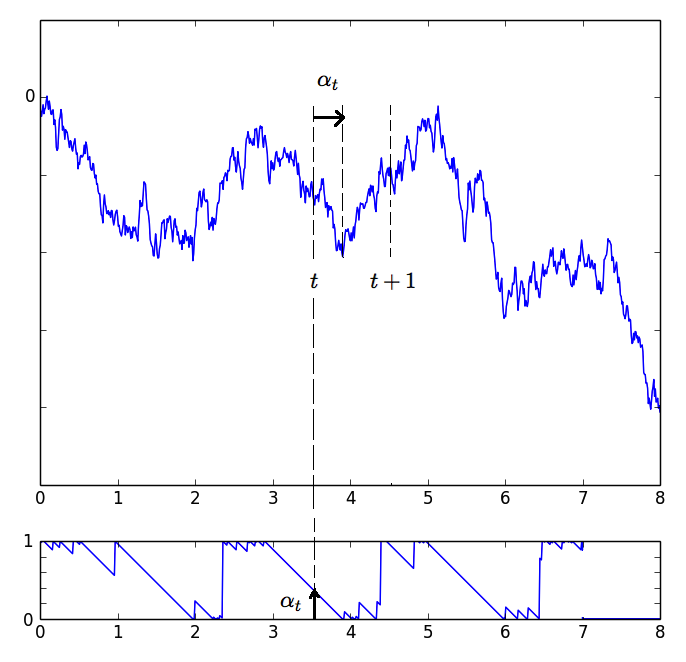
Figure 1: TOP: The argmin process embedded in Brownian motion. BOTTOM: The argmin process corresponding to the Brownian path on the top.

Let $(\Theta_{t};t\geq 0)$ be the $\mathcal{C}[0,\infty)$-valued space-time shift of Brownian motion $B$, defined by

$$\Theta_{t}:=(B_{t+u}-B_{t};u\geq 0)\quad\mbox{for all}~{}t\geq 0.$$

In the path space setting,

$$\alpha_{t}=\alpha_{0}\circ\Theta_{t}\quad\mbox{for all}~{}t\geq 0.$$ (2)

By the stationarity of $(\Theta_{t};t\geq 0)$, for any measurable function $g:\mathcal{C}[0,\infty)\rightarrow\mathbb{R}$, the process $(g\circ\Theta_{t};t\geq 0)$ is stationary. It is a well-known result of Lévy [33] that the time at which the minimum of Brownian motion on $[0,1]$ is achieved follows the arcsine distribution. As a result, we have the following proposition.

Proposition 1.1.

The argmin process $(\alpha_{t};t\geq 0)$ is stationary. The invariant measure is the arcsine distribution with density

$$f(x)=\frac{1}{\pi\sqrt{x(1-x)}}\quad\mbox{for}~{}0<x<1.$$ (3)

It is natural to ask whether $(\alpha_{t};t\geq 0)$ is a Markov process. Sufficient conditions for a function of a Markov process to be Markov are given by Dynkin [18], and Rogers and Pitman [44]. But these criteria do not apply to the argmin process, see Section 3.5. Nevertheless, we prove the following theorem.

Theorem 1.2.

The argmin process $(\alpha_{t};t\geq 0)$ is a Markov process with Feller transition semigroup $Q_{t}(x,\cdot)$, $t>0$ and $x\in[0,1]$ where

$$Q_{t}(x,dy)=\left\{\begin{array}[]{ccl}\displaystyle\frac{1_{\{0<y<1\}}}{\pi\sqrt{y(1-y)}}dy&\mbox{for}~{}0\leq x\leq 1<t,\\ \displaystyle\sqrt{\frac{1-x}{1-x+t}}\delta_{x-t}(dy)+\frac{\sqrt{(y+t-1)^{+}}}{\pi(y+t-x)\sqrt{1-y}}dy&\mbox{for}~{}0<t\leq x\leq 1\\ \displaystyle\frac{\sqrt{(1-x)(t-x)}+\sqrt{y(y+t-1)^{+}}}{\pi(y+t-x)\sqrt{y(1-y)}}dy&\mbox{for}~{}0\leq x<t\leq 1.\end{array}\right.$$ (4)

See Kallenberg [28, Chapter 19] for background on Feller semigroups of continuous-time Markov processes. The proof of Theorem 1.2 is given in Sections 3.2 and 3.4.

Our approach relies on Denisov’s decomposition and excursion theory, see Section 2. We also investigate the law of jumps of $(\alpha_{t};t\geq 0)$. In particular, we prove that the argmin process $\alpha$ has local times at levels $0$ and $1$, and provide a Lévy system of $(\alpha_{t};t\geq 0)$. These results imply that the argmin process $\alpha$ is a time-homogeneous Markov process with an explicit description in the framework of jumping Markov processes by Jacod and Skorokhod [27], following the study of piecewise deterministic Markov processes by Davis [15].

The motivation for considering the argmin process comes from the study of Brownian extrema with given length. In the second part of this paper we provide further insight into these extrema, following previous works of Neveu and Pitman [38], and Leuridan [32]. For $a,b>0$, let

$$\mathcal{M}_{a,b}:=\left\{t\geq a:B_{t}=\inf_{s\in[t-a,t+b]}B_{s}\right\}=\{T_{1}^{a,b},T^{a,b}_{2},\cdots\},$$ (5)

with $a<T_{1}^{a,b}<T^{a,b}_{2}<\cdots$ be the $(a,b)$-minima set of Brownian motion $B$.

The study of Brownian extrema dates back to Lévy [33]. See [29, Section 2.9] for development. Neveu and Pitman [38] proved the renewal property of Brownian local extrema by looking at Brownian extrema of a given depth. They gave the following Palm description of Brownian local extrema.

Theorem 1.3.

[38] Let $(\mathcal{C},\mathcal{B})$ be the space of continuous paths on $\mathbb{R}$, equipped with Wiener measure ${\bf W}$, and $(E,\mathcal{E})$ be the space of excursions with lifetime $\zeta$, equipped with Itô’s law ${\bf n}$ (see Section 2.2 for discussion). For $A\in\mathcal{B}$, define the $\sigma$-finite Palm measure of Brownian local minima by

$$\nu(A):=\mathbb{E}\#\{0\leq t\leq 1:t~{}\mbox{is a local minimum and}~{}\theta_{t}\in A\},$$ (6)

where $\theta_{t}:=(b_{t+u}-b_{t};t\in\mathbb{R})$ is the space-time shift of a two-sided Brownian motion $b$. Then for $A\in\mathcal{B}$,

$$\nu(A)=\frac{1}{2}({\bf n}\otimes{\bf n}\otimes{\bf W})(f^{-1}(A)),$$ (7)

where $f:E\times E\times\mathcal{C}\ni(e,e^{\prime},w)\rightarrow\widetilde{w}\in\mathcal{C}$ is a mapping given by

$$\widetilde{w}_{t}=\left\{\begin{array}[]{ccl}w_{t+\zeta(e^{\prime})}&\mbox{if}&t\leq-\zeta(e^{\prime}),\\ e^{\prime}_{-t}&\mbox{if}&-\zeta(e^{\prime})\leq t\leq 0,\\ e_{t}&\mbox{if}&0\leq t\leq\zeta(e),\\ w_{t-\zeta(e)}&\mbox{if}&t\geq\zeta(e).\end{array}\right.$$ (8)

The quantity $\nu(A)$ is interpreted as the mean number of Brownian local minima of type $A$ per unit time. See Kallenberg [28, Chapter 11] for background on Palm measures.

Neveu-Pitman’s results were generalized to Brownian motion with drift by Faggionato [20]. Inspired from [38], Leuridan [32] considered Brownian extrema with given length. In different directions, Groeneboom [24] considered the global extremum of Brownian motion with a parabolic drift, where he gave a density formula in terms of Airy functions. Tsirelson [50] provided an i.i.d. uniform sampling construction of Brownian local extrema under external randomization. Abramson and Evans [1] considered Lipschitz minorants of Brownian motion, which is a variant of Brownian extrema.

Leuridan studied the $(a,b)$-minima set $\mathcal{M}^{\prime}_{a,b}:=\{t\in\mathbb{R}:b_{t}=\inf_{s\in[t-a,t+b]}b_{s}\}$ of a two-sided Brownian motion $(b_{t};t\in\mathbb{R})$. He proved that times of the set $\mathcal{M}^{\prime}_{a,b}$ form a renewal process, and provided the density of the inter-arrival times. Observe that

$$\mathcal{M}_{a,b}-a\stackrel{{\scriptstyle(d)}}{{=}}\mathcal{M}^{\prime}_{a,b}\cap[0,\infty).$$ (9)

That is, $\mathcal{M}_{a,b}-a:=\{T_{i}^{a,b}-a;i\geq 1\}$ is a renewal process with stationary delay. We adapt Leuridan’s result to one-sided Brownian motion as follows.

Theorem 1.4.

[32] Let $a,b>0$. The times of $(a,b)$-minima of Brownian motion $(B_{t};t\geq 0)$ form a delayed renewal process, denoted by $(T_{i}^{a,b};i\geq 1)$ so that $a<T_{1}^{a,b}<T_{2}^{a,b}<\cdots$. Let

$$h_{a,b}(t):=\left\{\begin{array}[]{ccl}\displaystyle\frac{1}{\pi t}\left(\sqrt{\frac{(t-b)^{+}}{b}}+\sqrt{\frac{(t-a)^{+}}{a}}\right)&\mbox{for}&0<t<a+b\\ \displaystyle\frac{1}{\pi\sqrt{ab}}&\mbox{for}&t\geq a+b.\end{array}\right.$$ (10)

Then $(\Delta_{i}^{a,b}:=T_{i+1}^{a,b}-T_{i}^{a,b};i\geq 1)$ are independent, with density

$$g_{a,b}(t):=\sum_{n=1}^{\infty}(-1)^{n-1}h_{a,b}^{*n}(t),$$ (11)

where $h_{a,b}^{*n}$ is the $n^{th}$ convolution of $h_{a,b}$. In addition, $T_{1}^{a,b}$ is independent of $(\Delta_{i}^{a,b};i\geq 1)$, and has density

$$f_{a,b}(t):=\frac{1_{\{t>a\}}}{\pi\sqrt{ab}}\int_{t-a}^{\infty}g_{a,b}(s)ds.$$ (12)

Given a measurable set $A\subset\mathbb{R}^{+}$, let $N_{a,b}(A):=\#(\mathcal{M}_{a,b}\cap A)$ be the counting measure of $(a,b)$-minima in Brownian motion $B$. Leuridan’s proof of Theorem 1.4 is based on the formula, for $n\geq 1$ and $0<t_{1}<\cdots<t_{n}$,

$$\mathbb{E}(N_{a,b}(dt_{1})\cdots N_{a,b}(dt_{n}))=\frac{1}{\pi\sqrt{ab}}\prod_{k=1}^{n-1}h_{a,b}(t_{k}-t_{k-1})dt_{1}\cdots dt_{n},$$ (13)

with convention that $\prod_{\emptyset}:=1$. The case $n=1$ of (13) follows readily from Theorem 1.3, since for a generic $(a,b)$-minimum, the left excursion has length larger than $a$ and the right excursion has length larger than $b$. This implies that the mean number of $(a,b)$-minima per unit time is given by

$$\frac{1}{2}{\bf n}(\zeta(e^{\prime})>a){\bf n}(\zeta(e)>b)=\frac{1}{\pi\sqrt{ab}}.$$

In particular,

$$\mathbb{E}(\Delta_{i}^{a,b})=\pi\sqrt{ab}\quad\mbox{for all}~{}i\geq 1.$$ (14)

However, to obtain (13) for $n\geq 2$ requires extra work. Observe that for $a+b=1$, the set $\mathcal{M}_{a,b}$ can be viewed as the $a$-level set of the argmin process $\alpha$. So by Brownian scaling,

$$\mathcal{M}_{a,b} \stackrel{{\scriptstyle(d)}}{{=}}(a+b)\mathcal{M}_{\frac{a}{a+b},\frac{b}{a+b}}$$

$$\stackrel{{\scriptstyle(d)}}{{=}}(a+b)\alpha^{-1}\left(\left\{\frac{a}{a+b}\right\}\right)\quad\mbox{for}~{}a,b>0.$$ (15)

According to Hoffmann-Jørgensen [25], and Krylov and Juškevič [31], the set $\mathcal{M}_{a,b}$ enjoys regenerative property, and is called a strong Markov set. See also Kingman [30] for a survey on regenerative phenomena of level sets of Markov processes. In Section 4.1, we recover Theorem 1.4, in particular (13), by using the properties of the argmin process $\alpha$.

Note that the density $h_{a,b}$ defined by (10) is induced by a $\sigma$-finite measure. By Leuridan’s formula (11), the Laplace transform of $\Delta^{a,b}_{i}$ is given by

$$\Phi_{\Delta^{a,b}}(\lambda)=\frac{\Psi(\lambda)}{1+\Psi(\lambda)}\quad\mbox{with}~{}\Psi(\lambda):=\int_{0}^{\infty}e^{-\lambda t}h_{a,b}(t)dt,$$ (16)

provided that $\Psi(\lambda)<1$. By analytic continuation, we extend (16) to all $\lambda>0$. But it does not seem obvious how to simplify (16) analytically.

While the description of $\mathcal{M}_{a,b}$ is complicated for general $a,b>0$, the case $a=b$ is simplified. For simplicity, we consider $a=b=1$. We shall give a construction of the $(1,1)$-minima set

$$\mathcal{M}_{1,1}:=\{T_{1},T_{2},\cdots\}\quad\mbox{with}~{}1<T_{1}<T_{2}<\cdots,$$

from which we derive simple formulas for the Laplace transforms of $\Delta_{i}:=T_{i+1}-T_{i}$ and $T_{1}$.

Let $J$ be the first descending ladder time of Brownian motion, from which starts an excursion above the minimum of length larger than $1$. It is known that the Laplace transform of $J$ is given by

$$\Phi_{J}(\lambda)=\frac{1}{\sqrt{\pi\lambda}\operatorname{erf}(\sqrt{\lambda})+e^{-\lambda}},$$ (17)

where $\operatorname{erf}(x):=\frac{2}{\sqrt{\pi}}\int_{0}^{x}e^{-t^{2}}dt$ is the error function. See Proposition 2.3 for a derivation of (17).

The random variable $J$ plays an important role in our construction of the $(1,1)$-minima set. Let $\Delta$ be distributed as the law of the inter-arrival times $\Delta_{i}$, independent of $J$. It is a simple consequence of the construction in Section 4.2 of the Brownian path over $[0,T_{1}]$ and over $[T_{i},T_{i+1}]$ that

$$T_{1}\stackrel{{\scriptstyle(d)}}{{=}}J+1_{\{J<1\}}\Delta,\quad\mbox{with}~{}J~{}\mbox{independent of}~{}\Delta.$$ (18)

Combined with the fact that $T_{1}-1$ is the stationary delay for a renewal process with inter-arrival time distributed according to $\Delta$, this leads to the following result:

Theorem 1.5.

Let $(T_{i};i\geq 1)$ with $1<T_{1}<T_{2}<\cdots$ be times of the $(1,1)$-minima set $\mathcal{M}_{1,1}$ of Brownian motion $B$.

1. Let $J^{\prime}$ be an independent copy of $J$, whose Laplace transform is given by (17). Then there is the identity in law

   $$T_{1}-1\stackrel{{\scriptstyle(d)}}{{=}}J+J^{\prime}.$$ (19)

   In particular, the Laplace transforms of $T_{1}$ and $\Delta$ are given by

   $$\Phi_{T_{1}}(\lambda)=\frac{e^{-\lambda}}{(\sqrt{\pi\lambda}\operatorname{erf}(\sqrt{\lambda})+e^{-\lambda})^{2}},$$ (20)

   and

   $$\Phi_{\Delta}(\lambda)=1-\frac{\pi\lambda}{(\sqrt{\pi\lambda}\operatorname{erf}(\sqrt{\lambda})+e^{-\lambda})^{2}}.$$ (21)

   Consequently,

   $$\mathbb{E}T_{1}=3\quad\mbox{and}\quad\mathbb{E}\Delta=\pi.$$ (22)

2. The fragments $(B_{T_{i}+t}-B_{T_{i}};0\leq t\leq\Delta_{i})_{i\geq 1}$, are i.i.d., starting as Brownian meander of length $1$, and then running as Brownian motion until the next $(1,1)$-minima occurs.

   $$\mathbb{E}B_{T_{1}}=-\sqrt{\frac{\pi}{2}}\quad\mbox{and}\quad\operatorname{Var}B_{T_{1}}=\frac{4+\pi}{2},$$ (23)

   and

   $$\mathbb{E}(B_{T_{i+1}}-B_{T_{i}})=0\quad\mbox{and}\quad\operatorname{Var}(B_{T_{i+1}}-B_{T_{i}})=\pi~{}\mbox{for all}~{}i\geq 1.$$ (24)

In Section 4.2, we prove the identity in law (19) by computing the Laplace transform (20) of $T_{1}$. This identity in law is surprising, and we do not have a simple explanation. Though we are able to compute the first two moments (23)-(24), the laws of $B_{T_{1}}$, and $B_{T_{i+1}}-B_{T_{i}}$ seem to be difficult. We leave these for further investigation.

Recall the notations in Theorem 1.3. For $a>0$, let

$$\nu^{a}(A):=\mathbb{E}\#\{0\leq t\leq 1:t\in\mathcal{M}^{\prime}_{a,a}~{}\mbox{and}~{}\theta_{t}\in A\}\quad\mbox{for}~{}A\in\mathcal{B},$$

be the Palm measure of $(a,a)$-minima of a two-sided Brownian motion. Theorem 1.5 implies that $\nu^{a}$ has total mass $\frac{1}{\pi a}$, and

$$\nu^{a}(A)=\frac{1}{2}1_{\{\zeta^{\prime}>a,\zeta>a\}}({\bf n\otimes n\otimes W})(f^{-1}(A))\quad\mbox{for}~{}A\in\mathcal{B},$$ (25)

where $f$ is the mapping defined by (8). By taking $a\downarrow 0$, the Palm measures $\nu^{a}$ increase to the limit $\nu$ defined by (7). This recovers Theorem 1.3.

The set $\mathcal{M}_{1,1}$ is directly related to the argmin process $\alpha$ without scaling. In fact, $T_{i}$ is the $i^{th}$ time that the process $\alpha$ reaches $0$ by a continuous passage from $1$. So the law of Brownian fragments between $(1,1)$-minima can be derived from the study of $\alpha$. Let

$$\mathcal{LE}:=\{t\geq 0:B_{t}<B_{s},~{}\mbox{for all}~{}s\in[t,t+1]\},$$

be the left ends of forward meanders of length $1$, and

$$\mathcal{RE}:=\{t\geq 1:B_{t}<B_{s},~{}\mbox{for all}~{}s\in[t-1,t]\},$$

be the right ends of backward meanders of length $1$. In Lemma 4.10, we show that left ends come before right ends between any two consecutive $(1,1)$-minima. So we define for each $i\geq 1$,

$$D_{i}:=\inf\{t>T_{i}:t\in\mathcal{RE}\}\quad\mbox{and}\quad G_{i}:=\sup\{t<D_{i}:t\in\mathcal{LE}\}.$$ (26)

For each $i\geq 1$, the triple $(G_{i}-T_{i},D_{i}-G_{i},T_{i+1}-D_{i})$ gives a decomposition of $\Delta_{i}$:

$$\Delta_{i}=(G_{i}-T_{i})+(D_{i}-G_{i})+(T_{i+1}-D_{i}).$$ (27)

By using the Lévy system of the argmin process, we prove the following theorem which identifies the law of this triple.

Theorem 1.6.

For each $i\geq 1$, $G_{i}-T_{i}$, $D_{i}-G_{i}$ and $T_{i+1}-D_{i}$ are mutually independent, with

• $G_{i}-T_{i}\stackrel{{\scriptstyle(d)}}{{=}}T_{i+1}-D_{i}\stackrel{{\scriptstyle(d)}}{{=}}J$, the Laplace transform of which is given by (17);

• the density of $D_{i}-G_{i}$ is given by

  $$\mathbb{P}(D_{i}-G_{i}\in dt)=\frac{2-t}{t^{2}\sqrt{t-1}}1_{\{1<t<2\}}dt.$$ (28)

  Consequently, for each $i\geq 1$,

  $$\mathbb{E}(G_{i}-T_{i})=\mathbb{E}(T_{i+1}-D_{i})=1\quad\mbox{and}\quad\mathbb{E}(D_{i}-G_{i})=\pi-2.$$ (29)

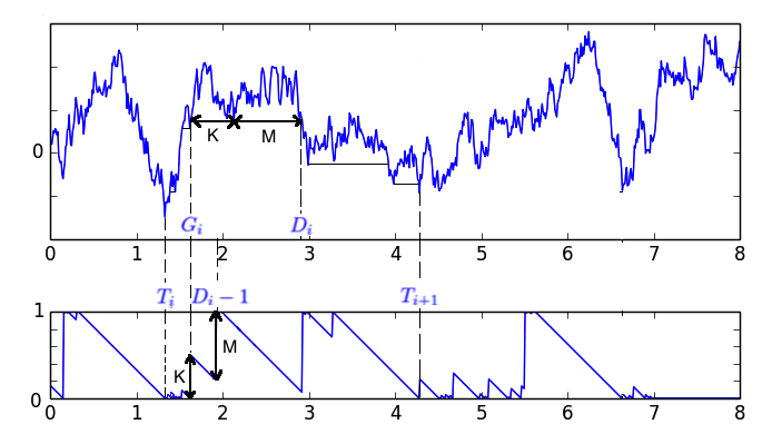
Figure 2: $(T_{i},G_{i},D_{i},T_{i+1})$ related to the argmin process $(\alpha_{t};t\geq 0)$.

For a random variable $X$, let $\Phi_{X}(\lambda)$ be the Laplace transform of $X$, and $f_{X}(\cdot)$ be the density of $X$. Theorems 1.4-1.6 provide three different descriptions of the inter-arrival time $\Delta$. This leads to some non-trivial identities. We summarize the results in the following table.

	Laplace transform $\Phi_{X}(\lambda)$	Density $f_{X}(t)$
$X=J$, Prop 2.3	$\displaystyle\frac{1}{\sqrt{\pi\lambda}\operatorname{erf}(\sqrt{\lambda})+e^{-\lambda}}$	Given by (54)
$X=D-G$, Th 1.6	$\displaystyle\pi\lambda\left[(\operatorname{erf}(\sqrt{\lambda})^{2}-1)\right]+2\sqrt{\pi\lambda}e^{-\lambda}\operatorname{erf}(\sqrt{\lambda})+e^{-2\lambda}$	$\displaystyle\frac{2-t}{t^{2}\sqrt{t-1}}1_{\{1<t<2\}}$
$X=\Delta$, Th 1.4	$\displaystyle\frac{\Psi(\lambda)}{1+\Psi(\lambda)}$, with	Given by (11),
	$\displaystyle\Psi(\lambda)=\operatorname{erf}(\sqrt{\lambda})^{2}-1+\frac{2e^{-\lambda}}{\sqrt{\pi\lambda}}\operatorname{erf}(\sqrt{\lambda})+\frac{e^{-2\lambda}}{\pi\lambda}$	with $a=b=1$
$X=\Delta$, Th 1.5	$\displaystyle 1-\pi\lambda(\Phi_{J}(\lambda))^{2}$	$\displaystyle-\pi\frac{d}{dt}f^{*2}_{J}(t)$
$X=\Delta$, Th 1.6	$\displaystyle(\Phi_{J}(\lambda))^{2}\Phi_{D-G}(\lambda)$	$(f_{J}*f_{D-G}*f_{J})(t)$
$X=T_{1}-1$, Th 1.4	$\displaystyle\frac{1}{\pi\lambda}(1-\Phi_{\Delta}(\lambda))$	$\displaystyle\frac{1_{\{t>0\}}}{\pi}\int_{t}^{\infty}f_{\Delta}(s)ds$
$X=T_{1}-1$, Th 1.5	$\displaystyle(\Phi_{J}(\lambda))^{2}$	$f_{J}^{*2}(t)$

TABLE $1$. Laplace transforms and densities.

Finally, we extend Theorem 1.2 to random walks and Lévy processes. Fix $N\geq 1$. We study the argmin process $(A_{N}(n);n\geq 0)$ of a random walk $(S_{n};n\geq 0)$, defined by

$$A_{N}(n):=\sup\left\{1\leq i\leq N;S_{n+i}=\min_{1\leq i\leq N}S_{n+i}\right\}\quad\mbox{for all}~{}n\geq 0,$$ (30)

where $S_{n}:=\sum_{i=1}^{n}X_{i}$ is the $n^{th}$ partial sum of $(X_{n};n\geq 1)$ (with convention $S_{0}:=0$), and $(X_{n};n\geq 1)$ is a sequence of independent and identically distributed random variables with the cumulative distribution function $F$. This is the discrete analog of the argmin process of Brownian motion. A similar argument as in the Brownian case shows that $(A_{N}(n);n\geq 0)$ is a Markov chain. For $n\geq 1$, let

$$p_{n}:=\mathbb{P}(S_{1}\geq 0,\cdots,S_{n}\geq 0)\quad\mbox{and}\quad\widetilde{p}_{n}:=\mathbb{P}(S_{1}>0,\cdots,S_{n}>0).$$

Theorem 5.2 below recalls the classical theory of how the two sequences of probabilities $p_{n}$ and $\widetilde{p}_{n}$ are determined by the sequences of probabilities $\mathbb{P}(S_{n}\geq 0)$ and $\mathbb{P}(S_{n}>0)$. We give the transition matrix of the argmin chain $A_{N}$ in terms of $(p_{n};n\geq 1)$ and $(\widetilde{p}_{n};n\geq 1$), which can be made explicit for special choices of $F$.

Theorem 1.7.

Whatever the common distribution $F$ of $(X_{n};n\geq 0)$, the argmin chain $(A_{N}(n);n\geq 0)$ is a stationary and time-homogeneous Markov chain on $\{0,1,\ldots,N\}$. Let $\Pi_{N}(k)$, $k\in[0,N]$ be the stationary distribution, and $P_{N}(i,j)$, $i,j\in[0,N]$ be the transition probabilities of the argmin chain $(A_{N}(n);n\geq 0)$ on $[0,N]$. Then

$$\Pi_{N}(k)=p_{k}\widetilde{p}_{N-k}\quad\mbox{for}~{}0\leq k\leq N;$$ (31)

$$P_{N}(i,N)=1-\frac{\widetilde{p}_{N+1-i}}{\widetilde{p}_{N-i}}\quad\mbox{and}\quad P_{N}(i,i-1)=\frac{\widetilde{p}_{N+1-i}}{\widetilde{p}_{N-i}}\quad\mbox{for}~{}0<i\leq N;$$ (32)

$$P_{N}(0,j)=\frac{(p_{j}-p_{j+1})\widetilde{p}_{N-j}}{\widetilde{p}_{N}}\quad\mbox{for}~{}0\leq j<N\quad\mbox{and}\quad P_{N}(0,N)=1-\sum_{j=0}^{N-1}P_{N}(0,j).$$ (33)

Consequently,

1. If $(S_{n};n\geq 0)$ is a random walk with continuous distribution and $\mathbb{P}(S_{n}>0)=\theta\in(0,1)$ for all $n\geq 1$. Let $(\theta)_{n\uparrow}:=\prod_{i=0}^{n-1}(\theta+i)$ be the Pochhammer symbol. Then

   $$\Pi_{N}(k)=\frac{(\theta)_{k\uparrow}(\theta)_{N-k\uparrow}}{k!(N-k)!}\quad\mbox{for}~{}0\leq k\leq N;$$ (34)

   $$P_{N}(i,N)=\frac{1-\theta}{N+1-i}\quad\mbox{and}\quad P_{N}(i,i-1)=\frac{N+\theta-i}{N+1-i}\quad\mbox{for}~{}0<i\leq N;$$ (35)

   $$P_{N}(0,j)=\frac{1-\theta}{j+1}\binom{N}{j}\frac{(\theta)_{j\uparrow}(\theta)_{N-j\uparrow}}{(\theta)_{N\uparrow}}\quad\mbox{for}~{}0\leq j<N;$$ (36)

   and

   $$P_{N}(0,N)=\frac{2(1-\theta)}{N+1}-\frac{(1-2\theta)(2\theta)_{N\uparrow}}{(N+1)(\theta)_{N\uparrow}}.$$ (37)

2. If $(S_{n};n\geq 0)$ is a simple symmetric random walk. Let $\lfloor x\rfloor$ be the integer part of $x$. Then

   $$\Pi_{N}(k)=\frac{\displaystyle\left(\frac{1}{2}\right)_{\lfloor{\frac{k+1}{2}}\rfloor\uparrow}\left(\frac{1}{2}\right)_{\lfloor\frac{N-k}{2}\rfloor\uparrow}}{\displaystyle 2\cdot\left\lfloor\frac{k+1}{2}\right\rfloor!\left\lfloor\frac{N-k}{2}\right\rfloor!}\quad\mbox{for}~{}0\leq k\leq N;$$ (38)

   For $0<i\leq N$,

   $$P_{N}(i,N)=\left\{\begin{array}[]{ccl}\frac{N-i}{N+1-i}&\mbox{if}~{}N-i~{}\mbox{is odd};\\[8.0pt] 1&\mbox{if}~{}N-i~{}\mbox{is even};\end{array}\right.\mbox{and}~{}P_{N}(i,i-1)=1-P_{N}(i,N);$$ (39)

   for $0\leq j<N$,

   $$P_{N}(0,j)=\left\{\begin{array}[]{ccl}0&\mbox{if}~{}j~{}\mbox{is odd};\\[8.0pt] \frac{\displaystyle\binom{j}{\frac{j}{2}}\binom{2\lfloor\frac{N}{2}\rfloor-j}{\lfloor\frac{N}{2}\rfloor-\frac{j}{2}}}{\displaystyle(j+2)\binom{2\lfloor\frac{N}{2}\rfloor}{\lfloor\frac{N}{2}\rfloor}}&\mbox{if}~{}j~{}\mbox{is even};\end{array}\right.$$ (40)

   and

   $$P_{N}(0,N)=\left\{\begin{array}[]{ccl}\frac{1}{N+1}&\mbox{if}~{}N~{}\mbox{is odd};\\[8.0pt] \frac{2}{N+2}&\mbox{if}~{}N~{}\mbox{is even}.\end{array}\right.$$ (41)

For the argmin chain $A_{N}$, the transition probability from $0$ to $N$ is given by (33) in the general case. But this probability is simplified to (37) and (41) in the two special cases. These identities are proved analytically by Lemmas 5.4 and 5.7. We do not have a simple explanation, and leave combinatorial interpretations for the readers.

Let $(X_{t};t\geq 0)$ be a real-valued Lévy process. We consider the argmin process $(\alpha_{t}^{X};t\geq 0)$ of $X$, defined by

$$\alpha_{t}^{X}:=\sup\left\{s\in[0,1]:X_{t+s}=\inf_{u\in[0,1]}X_{t+u}\right\}\quad\mbox{for all}~{}t\geq 0.$$ (42)

We are particularly interested in the case where $X$ is a stable Lévy process. We follow the notations in Bertoin [5, Chapter VIII]. Up to a multiple factor, a stable Lévy process $X$ is entirely determined by a scaling parameter $\alpha\in(0,2]$, and a skewness parameter $\beta\in[-1,1]$. The characteristic exponent of a stable Lévy process $X$ with parameters $(\alpha,\beta)$ is given by

$$\Psi(\lambda):=\left\{\begin{array}[]{ccl}|\lambda|^{\alpha}(1-i\beta\operatorname{sgn}(\lambda)\tan(\pi\alpha/2))&\mbox{for}~{}\alpha\neq 1,\\[8.0pt] |\lambda|(1+i\frac{2\beta}{\pi}\operatorname{sgn}(\lambda)\log|\lambda|)&\mbox{for}~{}\alpha=1\end{array}\right.$$

where $\operatorname{sgn}$ is the sign function. Let $\rho:=\mathbb{P}(X_{1}>0)$ be the positivity parameter. Zolotarev [53, Section 2.6] found that

$$\rho=\frac{1}{2}+(\pi\alpha)^{-1}\arctan(\beta\tan(\pi\alpha/2))\quad\mbox{for}~{}\alpha\in(0,2].$$ (43)

If $X$ (resp. $-X$ ) is a subordinator, then almost surely $\alpha^{X}_{t}=0$ (resp. $\alpha^{X}_{t}=1$) for all $t\geq 0$. The following theorem is a generalization of Theorem 1.2.

Theorem 1.8.

1. Let $(X_{t};t\geq 0)$ be a Lévy process. Then the argmin process $(\alpha^{X}_{t};t\geq 0)$ of $X$ is a stationary and time-homogeneous Markov process.

2. Let $(X_{t};t\geq 0)$ be a stable Lévy process with parameters $(\alpha,\beta)$, and assume that neither $X$ nor $-X$ is a subordinator. Let $\rho$ be defined by (43). Then the argmin process $(\alpha^{X}_{t};t\geq 0)$ of $X$ has generalized arcsine distributed invariant measure whose density is

   $$f(x):=\frac{\sin\pi\rho}{\pi}x^{-\rho}(1-x)^{\rho-1}\quad\mbox{for}~{}0<x<1,$$ (44)

   and Feller transition semigroup $Q^{X}_{t}(x,\cdot)$, $t>0$ and $x\in[0,1]$ where

   $$Q^{X}_{t}(x,dy)=\left\{\begin{array}[]{ccl}1_{\{0<y<1\}}\frac{\sin\pi\rho}{\pi}y^{-\rho}(1-y)^{\rho-1}dy&\mbox{for}~{}0\leq x\leq 1<t,\\[8.0pt] \left(\frac{1-x}{1-x+t}\right)^{1-\rho}\delta_{x-t}(dy)+\frac{\sin\pi\rho}{\pi}\cdot\frac{(1-y)^{\rho-1}(y+t-1)_{+}^{\rho}}{(y+t-x)}dy&\mbox{for}~{}0<t\leq x\leq 1,\\[8.0pt] \frac{\sin\pi\rho}{\pi(y+t-x)}y^{-\rho}(1-y)^{\rho-1}[(t-x)^{\rho}(1-x)^{1-\rho}+y^{\rho}(y+t-1)_{+}^{1-\rho}]dy&\mbox{for}~{}0\leq x<t\leq 1.\end{array}\right.$$ (45)

Organization of the paper: The layout of the paper is as follows.

• In Section 2, we provide background and necessary tools which will be used later.

• In Section 3, we study the argmin process $(\alpha_{t};t\geq 0)$ of Brownian motion, and prove Theorem 1.2.

• In Section 4, we study the $(a,b)$-minima of Brownian motion with an emphasis on the case $a=b=1$. There we prove Theorems 1.4, 1.5 and 1.6.

• In Section 5, we consider the argmin process of random walks and Lévy processes, and prove Theorems 1.7 and 1.8.

2 Background and tools

This section recalls some background of Brownian motion. In Section 2.1, we consider Denisov’s decomposition for Brownian motion. In Section 2.2, we recall various results from Brownian excursion theory.

2.1 Path decomposition of Brownian motion

Let $(B_{t};t\geq 0)$ be standard Brownian motion. A Brownian meander $(m_{t};0\leq t\leq 1)$ can be regarded as the weak limit of

$$\left(B_{t};0\leq t\leq 1\Bigg{|}\inf_{0\leq s\leq 1}B_{s}>-\epsilon\right)\quad\mbox{as}~{}\epsilon\downarrow 0.$$

We refer to Durrett et al. [17] for a proof. A Brownian meander of length $x$, say $(m^{x}_{t};0\leq t\leq x)$ is defined as

$$m^{x}_{t}:=\sqrt{x}m_{t/x}\quad\mbox{for}~{}0\leq t\leq x.$$

In particular, $m^{x}_{x}$ is Rayleigh distributed with scale parameter $\sqrt{x}$. That is,

$$\mathbb{P}(m^{x}_{x}\in dy)=\frac{y}{x}\exp\left(-\frac{y^{2}}{2x}\right)dy\quad\mbox{for}~{}y>0.$$ (46)

Consequently,

$$\mathbb{E}m^{x}_{x}=\sqrt{\frac{\pi x}{2}}\quad\mbox{and}\quad\operatorname{Var}m^{x}_{x}=\frac{4-\pi}{2}x.$$ (47)

The following path decomposition is due to Denisov.

Theorem 2.1 (Denisov’s decomposition for Brownian motion, [16]).

Let $A:=\operatorname{argmin}_{u\in[0,1]}B_{u}$ be the time at which Brownian motion $B$ attains its minimum on $[0,1]$. Given $A$, which is arcsine distributed, the Brownian path is decomposed into two conditionally independent pieces:

1. $(B_{A-t}-B_{A};0\leq t\leq A)$ is a Brownian meander of length $A$;

2. $(B_{A+t}-B_{A};0\leq t\leq 1-A)$ is a Brownian meander of length $1-A$.

Let

$${\bf P}^{x}:=\overset{\longleftarrow}{{\bf M}^{x}}\otimes\overset{\longrightarrow}{{\bf M}^{1-x}}\otimes{\bf W}\quad\mbox{for}~{}0\leq x\leq 1$$ (48)

be the law of two independent Brownian meanders of length $x$ and $1-x$ joined back-to-back, concatenated by an independent Brownian path running forever. Denisov’s decomposition is equivalent to

$${\bf W}(\cdot)=\int_{0}^{1}\frac{1}{\pi\sqrt{x(1-x)}}{\bf P}^{x}(\cdot)dx.$$ (49)

2.2 Brownian excursion theory

Let $(B_{t};t\geq 0)$ be standard Brownian motion, and $\underline{B}_{t}:=\inf_{0\leq s\leq t}B_{s}$ be the past-minimum process of $B$. For $l>0$, let $T_{l}:=\inf\{t>0;B_{t}<-l\}$ be the first time at which $B$ hits below level $-l$. Let

$$\mathcal{D}:=\{l>0:T_{l-}<T_{l}\},$$

so that for $l\in\mathcal{D}$,

$$e_{l}:=\left\{\begin{array}[]{cll}B_{T_{l-}+t}-\underline{B}_{T_{l-}+t}&\mbox{for}~{}0\leq t\leq T_{l}-T_{l-}\\ 0&\mbox{for}~{}t>T_{l}-T_{l-}\end{array}\right.$$

is an excursion away from $-l$. Let $E$ be the space of excursions defined by

$$E:=\{\epsilon\in\mathcal{C}[0,\infty);\epsilon_{0}=0,~{}\epsilon_{t}>0~{}\mbox{for}~{}t\in(0,\zeta(\epsilon)),~{}\mbox{and}~{}\epsilon_{t}=0~{}\mbox{for}~{}t\geq\zeta(\epsilon)\},$$

where $\zeta(\epsilon):=\inf\{t>0;\epsilon_{t}=0\}\in(0,\infty)$ is the lifetime of the excursion $\epsilon\in E$. The following theorem is a special case of Itô’s excursion theory.

Theorem 2.2.

[26] The point measure

$$\sum_{l\in\mathcal{D}}\delta_{(l,e_{l})}(dsd\epsilon)$$

is a Poisson point process on $\mathbb{R}^{+}\times E$ with intensity $ds\times{\bf n}(d\epsilon)$, where ${\bf n}(d\epsilon)$, called Itô’s excursion law, is a $\sigma$-finite measure on $E$.

Here we consider positive excursions of the reflected process $B-\underline{B}$. So the measure ${\bf n}(d\epsilon)$ corresponds to $2{\bf n}^{+}(d\epsilon)$ defined in Revuz and Yor [43, Chapter XII].

Let $\Lambda(dx)$ be the Lévy measure of a $\frac{1}{2}-$stable subordinator such that

$$\Lambda(dx)=\frac{dx}{\sqrt{2\pi x^{3}}}\quad\mbox{and}\quad\Lambda(x,\infty)=\sqrt{\frac{2}{\pi x}}\quad\mbox{for}~{}x>0.$$ (50)

By applying the master formula of Poisson point processes, we know that

$${\bf n}(\zeta\in dx)=\Lambda(dx).$$ (51)

See Revuz and Yor [43, Chapter XII] for development of Brownian excursion theory. Let

$$A_{t}:=\sum_{l}1_{\{T_{l-}\leq t\leq T_{l}\}}(t-T_{l-}),$$ (52)

be the age process of excursions of $B-\underline{B}$, or equivalently of a $\frac{1}{2}$-stable subordinator. The following proposition gathers useful results of $J$, defined by

$$J+1:=\inf\{t>0:A_{t}=1\}.$$

That is, $J$ is the first descending ladder time of Brownian motion, from which starts an excursion above the minimum of length exceeding $1$. For completeness, we include a proof.

Proposition 2.3.

[42] Let $J$ be the first descending ladder time of Brownian motion, from which starts an excursion above the minimum of length exceeding $1$.

1. The random variable $\frac{1}{1+J}$ has the same distribution as the longest interval of Poisson-Dirichlet $(\frac{1}{2},0)$ distribution. The Laplace transform of $J$ is given by (17), and

   $$\mathbb{E}J=1.$$ (53)

2. The density of $J$ is given by

   $$\frac{\mathbb{P}(J\in dt)}{dt}=\sum_{n=1}^{\infty}(-1)^{n+1}\frac{c_{n}}{\sqrt{t}}I_{n}\left(\frac{1}{1+t}\right)\quad\mbox{for}~{}t>0,$$ (54)

   where for each $n\geq 1$,

   $$c_{n}:=\frac{(n-1)!}{2^{n-1}\pi^{n/2}\Gamma(n/2)},$$

   and $I_{n}$ is a function supported on $(0,\frac{1}{n}]$ defined by

   $$I_{n}(u_{n}):=\int\prod_{i=1}^{n-1}\sqrt{\frac{(1-u_{i})^{n-1-i}}{u_{i}^{3}}}1_{\left\{\frac{u_{i+1}}{1-u_{i+1}}\leq u_{i}\leq\frac{1}{i}\right\}}du_{i}\quad\mbox{for}~{}u_{n}\in\left(0,\frac{1}{n}\right],$$

   with convention that $I_{1}(u_{1}):=1$ for $u_{1}\in(0,1]$. Consequently,

   $$\mathbb{P}(J\in dt)=\frac{dt}{\pi\sqrt{t}}\quad\mbox{for}~{}0<t\leq 1.$$ (55)

Proof 2.4.

The part $(1)$ is essentially from Pitman and Yor [42, Corollary 12] with $\alpha=\frac{1}{2}$. Alternatively, let $\tau:=\inf\{l\in D:T_{l}-T_{l-}>1\}$ be the first level above which an excursion has length larger than $1$ so that $J=T_{\tau-}$. As in [23], we deduce from Theorem 2.2 that $\tau$ is exponentially distributed with rate $\Lambda(1,\infty)=\sqrt{2/\pi}$, independent of $(B-\underline{B})[I_{\tau}]:=(B_{t}-\underline{B}_{t};t\in I_{\tau})$ and that

$$J\stackrel{{\scriptstyle(d)}}{{=}}\sigma_{\xi},$$

where

• $(\sigma_{t};t\geq 0)$ is a $\frac{1}{2}-$stable subordinator with all jumps of size larger than $1$ deleted, so the Laplace exponent of $(\sigma_{t};t\geq 0)$ is given by

  $$\phi(\lambda):=\int_{0}^{1}(1-e^{-\lambda x})\Lambda(dx)=\sqrt{2\lambda}\operatorname{erf}(\sqrt{\lambda})-\sqrt{\frac{2}{\pi}}(1-e^{-\lambda})\quad\mbox{for}~{}\lambda\geq 0.$$

• $\xi$ is exponentially distributed with rate $\sqrt{2/\pi}$, independent of $(\sigma_{t};t\geq 0)$.

So

$$\mathbb{E}J=\mathbb{E}\sigma_{1}\mathbb{E}\xi=\sqrt{\frac{2}{\pi}}\cdot\sqrt{\frac{\pi}{2}}=1,$$

and the Laplace transform of $J$ is given by

$$\Phi_{J}(\lambda)=\frac{\sqrt{2/\pi}}{\sqrt{2/\pi}+\phi(\lambda)}=\frac{1}{\sqrt{\pi\lambda}\operatorname{erf}(\sqrt{\lambda})+e^{-\lambda}}.$$

The part $(2)$ is obtained by specializing Pitman and Yor [42, Proposition 20] to $\alpha=\frac{1}{2}$ and $\theta=0$.

The following result can be read from Maisonneuve [34, Section 8] and Bolthausen [8]. An alternative approach was provided by Greenwood and Pitman [23], and Pitman [39, Sections 4 and 5].

Theorem 2.5.

[34, 8] The process

$$(B-\underline{B})[J,J+1]:=(B_{J+t}-\underline{B}_{J+t};0\leq t\leq 1)$$

is a Brownian meander of length $1$, independent of $(B_{u};0\leq u\leq J)$.

3 The argmin process of Brownian motion

In this section, we study the argmin process $\alpha$ of Brownian motion defined by (1). In Section 3.1, we deal with the sample path properties of $\alpha$. In Section 3.2, we provide a conceptual proof that the argmin process $\alpha$ is a Markov process with the Feller property. In Section 3.3, we study the jumps of $\alpha$ by means of a Lévy system. In Section 3.4, we compute the transition kernel of $\alpha$, and prove Theorem 1.2. Finally in Section 3.5, we explain why Dynkin’s criterion and the Rogers-Pitman criterion do not apply to the argmin process $\alpha$.

3.1 Sample path properties

We have mentioned in the introduction that the argmin process $(\alpha_{t};t\geq 0)$ takes values in $[0,1]$, and drifts down at unit speed except for positive jumps. More precisely, we provide the following proposition.

Proposition 3.1.

Let $(\alpha_{t};t\geq 0)$ be the argmin process of Brownian motion. Then a.s.

1. $\alpha_{t}\in[0,1]$ for all $t\geq 0$, and $(t+\alpha_{t};t\geq 0)$ is increasing;

2. $(\alpha_{t};t\geq 0)$ decreases at unit speed except for

   $(i)$ jumps from $0$ to some $x\in(0,1)$;

   $(ii)$ jumps from some $x\in(0,1)$ to $1$.

Proof 3.2.

(1) The fact $\alpha_{t}\in[0,1]$ is straightforward from the definition. Let $0\leq t<t^{\prime}$.

• If $t^{\prime}>t+\alpha_{t}$, then $t^{\prime}+\alpha_{t^{\prime}}>t+\alpha_{t}$.

• If $t^{\prime}\leq t+\alpha_{t}$, then $B_{t+\alpha_{t}}\leq B_{u}$ for all $u\in[t^{\prime},t+\alpha_{t}]$. This implies that $\alpha_{t^{\prime}}\geq t+\alpha_{t}-t^{\prime}$.

(2) Observe that $(\alpha_{t};t\geq 0)$ is a càdlàg process with only positive jumps. We first check $(i)$. If $\alpha_{t-}=0$ for some $t>0$, then $B_{u}\geq B_{t}$ for all $u\in[t,t+1]$. We distinguish two cases. In the first case, $B_{u}>B_{t}$ for all $u\in[t,t+1]$, which implies that $\alpha_{t}=0$. In the second case, $B_{u}=B_{t}$ for some $u\in(t,t+1]$, and let $x:=\sup\{u\in(0,1]:B_{t+u}=B_{t}\}$. If $x=1$, then there exists an excursion of length $1$ in Brownian motion by a space-time shift. But this is excluded by Pitman and Tang [41, Theorem 4]. Thus, $\alpha_{t}=x\in(0,1)$.

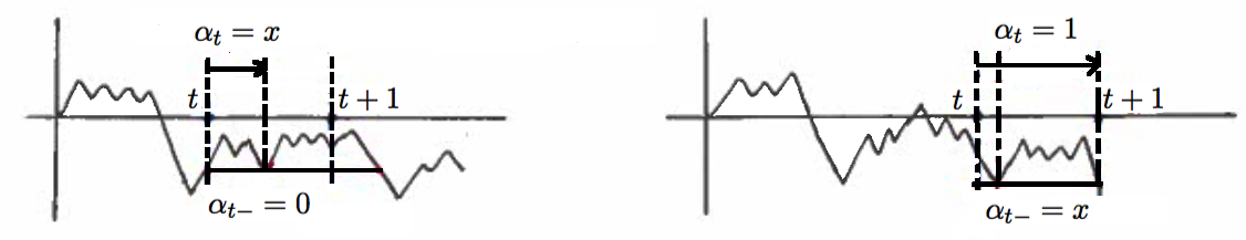
Figure 3: LEFT: A jump from $0$ to some $x\in(0,1)$ in the argmin process. RIGHT: A jump from some $x\in(0,1)$ to $1$ in the argmin process.

It remains to check $(ii)$. If $\alpha_{t-}=x\in(0,1)$ for some $t>0$, then $B_{t+x}<B_{u}$ for all $u\in(t+x,t+1)$. We also distinguish two cases. In the first case, $B_{t+1}>B_{t+x}$ which implies that $\alpha_{t}=x$. In the second case, $B_{t+1}=B_{t+x}$ which yields $\alpha_{t}=1$.

Next we prove a time reversal property of the argmin process $\alpha$. By convention, $\alpha_{0-}=\alpha_{0}$.

Proposition 3.3.

For each fixed $T>0$, $(1-\alpha_{(T-t)-};0\leq t\leq T)$ has the same distribution as $(\alpha_{t};0\leq t\leq T)$.

Proof 3.4.

Observe that $(1-\alpha_{(T-t)-};0\leq t\leq T)$ is also a càdlàg process. Let

$$\widetilde{B}:=(B_{T+1-u}-B_{T+1};0\leq u\leq T+1)\stackrel{{\scriptstyle(d)}}{{=}}(B_{u};0\leq u\leq T+1).$$

Let $\widetilde{\alpha}$ be the argmin process of $\widetilde{B}$ on $[0,T]$. Hence,

$$(1-\alpha_{(T-t)-};0\leq t\leq T)=(\widetilde{\alpha}_{t};0\leq t\leq T)\stackrel{{\scriptstyle(d)}}{{=}}(\alpha_{t};0\leq t\leq T).$$

3.2 Markov and Feller property

We provide a soft argument to prove that $(\alpha_{t};t\geq 0)$ is a Markov process, and enjoys the Feller property.

For each $t\geq 0$, let

$$\mathcal{G}_{t}:=\sigma(B_{s};0\leq s\leq t+\alpha_{t}),$$ (56)

be the $\sigma$-field generated by the path $B$ killed at time $t+\alpha_{t}$. By Proposition 3.1 (1), $t\mapsto t+\alpha_{t}$ is increasing. It is not hard to see that for any $s<t$, $s+\alpha_{s}$ is a measurable function of the path $B$ killed at $t+\alpha_{t}$. So $(\mathcal{G}_{t})_{t\geq 0}$ is a filtration. Now we show that

Proposition 3.5.

The argmin process $(\alpha_{t};t\geq 0)$ is time-homogeneous Markov with respect to $(\mathcal{G}_{t})_{t\geq 0}$.

Proof 3.6.

Fix $t>0$. By Denisov’s decomposition (Theorem 2.1), given $\alpha_{t}=x$ (i.e. the minimum of $B$ on $[t,t+1]$ is attained at $t+x$), the Brownian path is decomposed into four independent components:

• $(B_{t-s}-B_{t};0\leq s\leq t)$ is Brownian motion of length $t$;

• $(B_{t+x-s}-B_{t+x};0\leq s\leq x)$ is a Brownian meander of length $x$;

• $(B_{t+x+s}-B_{t+x};0\leq s\leq 1-x)$ is a Brownian meander of length $1-x$;

• $(B_{t+1+s}-B_{t+1};s\geq 0)$ is Brownian motion running forever.

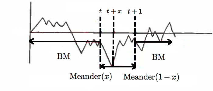
Figure 4: Decomposition of Brownian motion given $\alpha_{t}=x$.

As a consequence, $(B_{t+x+s}-B_{t+x};s\geq 0)$ and $(B_{t+x-s}-B_{t+x};0\leq s\leq t+x)$ are conditionally independent. Observe that given $\alpha_{t}=x$,

• for $s>t$, the minimum of $B$ on $[s,s+1]$ cannot be attained on $[s,t+x)$. So $(\alpha_{s};s>t)$ is entirely determined by the path $(B_{t+x+s}-B_{t+x};s\geq 0)$.

• for $s<t$, the minimum of $B$ on $[s,s+1]$ cannot be attained on $(t+x,s+1]$. So $(\alpha_{s};s<t)$ is entirely determined by the path $(B_{t+x-s}-B_{t+x};0\leq s\leq t+x)$.

These observations imply that $(\alpha_{t};t\geq 0)$ is Markov relative to $(\mathcal{G}_{t})_{t\geq 0}$. The time-homogeneity follows from the fact that given $\alpha_{t}=x$, the law of $(B_{t+x+s}-B_{t+x};s\geq 0)$ does not involve the time parameter $t$.

We now investigate the Feller property of the argmin process $(\alpha_{t};t\geq 0)$. Recall the definition of ${\bf P}^{x}$ from (48). Let

$$\alpha_{t}^{x}:=\alpha_{t}(B)\quad\mbox{for}~{}t\geq 0,$$ (57)

be the argmin process of $(B_{t};t\geq 0)$ under ${\bf P}^{x}$, which makes $\alpha_{0}=x\in[0,1]$. By Denisov’s decomposition (Theorem 2.1), for all $f:\mathcal{C}[0,\infty)\rightarrow\mathbb{R}$ bounded and continuous,

$$\mathbb{E}^{\bf W}f(\alpha_{t};t\geq 0)=\int_{0}^{1}\frac{dx}{\pi\sqrt{x(1-x)}}\mathbb{E}f(\alpha^{x}_{t};t\geq 0).$$

where $\mathbb{E}^{\bf W}$ is the expectation relative to ${\bf W}$.

The Feller property of $(\alpha_{t};t\geq 0)$ follows from a direct computation of the transition semigroup $Q_{t}(x,\cdot)$ of $(\alpha^{x}_{t};t\geq 0)$, which will be given in Section 3.4. But here we provide a conceptual proof.

Proposition 3.7.

The argmin process $(\alpha_{t};t\geq 0)$ enjoys the Feller property, and is a strong Markov process.

Proof 3.8.

According to Kallenberg [28, Lemma 19.3], it suffices to show that

1. for each $t\geq 0$, $\alpha_{t}^{x}\rightarrow\alpha_{t}^{y}$ in distribution as $x\rightarrow y$;

2. for each $x\in[0,1]$, $\alpha_{t}^{x}\rightarrow x$ in probability as $t\rightarrow 0$.

We first prove $(1)$. For $t\geq 1$, $\alpha_{t}^{x}$ and $\alpha_{t}^{y}$ are both arcsine distributed regardless of $x,y\in[0,1]$. Consider the case $t\in(0,1)$. By Denisov’s decomposition (Theorem 2.1), for all $f:\mathcal{C}[0,2]\rightarrow\mathbb{R}$ bounded and continuous,

$$\mathbb{E}^{\bf W}f(B_{u};0\leq u\leq 2)=\int_{0}^{1}\frac{dx}{\pi\sqrt{x(1-x)}}\mathbb{E}^{{\bf P}^{x}}f(B_{u};0\leq u\leq 2).$$

By the explicit scaling construction of Brownian meanders, the law of $(B_{u};0\leq u\leq 2)$ under ${\bf P}^{x}$ is weakly continuous in $x$. Moreover, for each $t\in(0,1)$, $\alpha_{t}(w)$ is an a.s. continuous functional of $(w_{u};0\leq u\leq 2)$, from which follows $(1)$.

It remains to prove $(2)$. Observe that for $t<1$, $1-t\leq\alpha_{t}^{1}\leq 1$. So $(2)$ is proved in case of $x=1$. For $x\in[0,1)$, by Denisov’s decomposition (Theorem 2.1),

$$\inf\{u\geq 1;w_{u}\leq w_{x}\}>1\quad{\bf P}^{x}\mbox{-}a.s.$$

Therefore, $\mathbb{P}(\alpha_{t}^{x}=x-t~{}\mbox{for}~{}t~{}\mbox{close to}~{}0)=1$, which leads to the desired result.

3.3 Jumps and Lévy system

We study the jumps of the argmin process $\alpha$. Recall the definitions of a $\frac{1}{2}-$stable subordinator, and the age process of a $\frac{1}{2}$-stable subordinator from (50) and (52). We begin with the following observation.

Lemma 3.9.

Let $\rho:=\inf\{t>0;\alpha_{t}=1\}$ and $\tau:=\inf\{t>\rho;\alpha_{t}=0\}$. Then $(1-\alpha_{\rho+t};0\leq t\leq\tau-\rho)$ has the same distribution as the age process of a $\frac{1}{2}-$stable subordinator until it first reaches $1$.

Proof 3.10.

By the strong Markov property of Brownian motion, $(B_{\rho+1+u}-B_{\rho+1};u\geq 0)$ is still Brownian motion. It is not hard to see that $(1-\alpha_{\rho+t};0\leq t\leq\tau-\rho)$ is the age process derived from excursions above the past minimum of $(B_{\rho+1+u}-B_{\rho+1};u\geq 0)$ until this post$-(\rho+1)$ Brownian motion escapes its past minimum by time $1$. This yields the desired result.

By Lemma 3.9, let $(l^{1}_{t};t\geq 0)$ be the local times of $\alpha$ at level $1$, normalized to match the $\frac{1}{2}-$stable subordinator. By time-reversal of $\alpha$ (Proposition 3.3), define similarly $(l^{0}_{t};t\geq 0)$ to be the local times of $\alpha$ at level $0$. By stationarity of $\alpha$,

$$\mathbb{E}l^{1}_{t}/t=\mathbb{E}l^{0}_{t}/t=c\quad\mbox{for all}~{}t>0.$$

We will prove in Corollary 4.17 that the constant $c=1/\sqrt{2\pi}$. These stationary local times also appeared in the work of Leuridan [32].

Before proceeding further, we need the following terminology. Let $(X_{t};t\geq 0)$ be a Hunt process on a suitably nice state space $E$, e.g. locally compact and separable metric space. The pair $(\Pi,C)$ constituted of a kernel $\Pi$ on $E$ and a continuous additive functional $C$ is said to be a Lévy system for $X$ if for all bounded and measurable function $f$ on $E\times E$,

$$\mathbb{E}\left(\sum_{0<s\leq t}f(X_{s-},X_{s})1_{\{X_{s-}\neq X_{s}\}}\right)=\mathbb{E}\left(\int_{0}^{t}dC_{s}\int_{E}\Pi(X_{s-},dy)f(X_{s-},y)\right).$$ (58)

The kernel $\Pi$ is called the Lévy measure of the additive functional $C$. The notion of a Lévy system was formulated by Watanabe [52], the existence of which was proved for a Hunt process under additional assumptions. The proof was simplified by Beneviste and Jacod [4]. See also Meyer [35], Pitman [39] and Sharpe [46, Chapter VIII] for development.

By Proposition 3.7, the argmin process $(\alpha_{t};t\geq 0)$ is a Hunt process. Also define a continuous additive functional $C$ by

$$C_{t}=t+l_{t}^{0}\quad\mbox{for}~{}t\geq 0.$$ (59)

The main result is stated as follows, the proof of which relies on Lemmas 3.12 and 3.15.

Theorem 3.11.

Let $(\alpha_{t};t\geq 0)$ be the argmin process of Brownian motion, and $(C_{t};t\geq 0)$ be the additive functional as in (59). Define a kernel $\Pi$ on $[0,1]$ by

$$\Pi(x,dy)=\left\{\begin{array}[]{ccl}\Pi^{0\uparrow}(dy)&\mbox{for}&x=0,\\ \mu^{\uparrow 1}(x)\delta_{1}&\mbox{for}&x\in(0,1),\\ 0&\mbox{for}&x=1.\end{array}\right.$$ (60)

where $\delta_{1}$ is the point mass at $1$,

$$\Pi^{0\uparrow}(dy):=\frac{dy}{\sqrt{2\pi y^{3}(1-y)}}\quad\mbox{for}~{}0<y<1,$$ (61)

and

$$\mu^{\uparrow 1}(x):=\frac{1}{2(1-x)}\quad\mbox{for}~{}0<x<1.$$ (62)

Then $(C,\Pi)$ is a Lévy system of $(\alpha_{t};t\geq 0)$.

Recall from Proposition 3.1 (2) that $(\alpha_{t};t\geq 0)$ can only have $(i).$ jumps from $0$ to some $x\in(0,1)$, and $(ii).$ jumps from some $x\in(0,1)$ to $1$. We start by computing the jump rate of $\alpha$ from $x\in(0,1)$ to 1.

Lemma 3.12.

Let $(\alpha_{t};t\geq 0)$ be the argmin process of Brownian motion.

1. Let $x>y\geq 0$. The probability that $\alpha^{x}$ decreases at unit speed from $x$ to $y$ with no jumps is given by

   $$s(x,y)=\sqrt{\frac{1-x}{1-y}}.$$ (63)

2. For $x\in(0,1)$, the jump rate of $\alpha$ per unit time from $x$ to $1$ is $\mu^{\uparrow 1}(x)$ defined by (62).

Proof 3.13.

$(1)$ Let $\widetilde{x}:=1-x$ and $\widetilde{y}:=1-y$. By Denisov’s decomposition (Theorem 2.1), under ${\bf P}^{x}$, $(B_{x+t}-B_{x};0\leq t\leq\widetilde{x})$ is a Brownian meander of length $\widetilde{x}$, independent of Brownian motion $(B_{1+t}-B_{1};t\geq 0)$.

Let $Z_{x-y}$ be normally distributed with mean $0$ and variance $x-y$. Let $R^{\widetilde{x}}$ be Rayleigh distributed with parameter $\widetilde{x}$, independent of $Z_{x-y}$. We have

$$s(x,y) ={\bf P}^{x}\left(\inf_{t\leq x-y}(B_{1+t}-B_{1})>B_{x}-B_{1}\right)$$

$$=\mathbb{P}(|Z_{x-y}|<R^{\widetilde{x}})$$

$$=2\int_{0}^{\infty}\mathbb{P}(R^{\widetilde{x}}>z)\cdot\frac{1}{\sqrt{2\pi(x-y)}}\exp\left(-\frac{z^{2}}{2(x-y)}\right)dz=\sqrt{\frac{\widetilde{x}}{\widetilde{y}}},$$

where the second equality follows from the reflection principle of Brownian motion, and the fact that a Brownian meander of length $\widetilde{x}$ evaluated at time $\widetilde{x}$ is Rayleigh distributed with parameter $\widetilde{x}$, whose density is given by (46).

$(2)$ Note that

$$s(x,y):=\exp\left(-\int_{y}^{x}dz\mu^{\uparrow 1}(z)\right).$$

We obtain the jump rate (62) by taking derivative of (63) with respect to $x$.

Remark 3.14.

We provide an alternative approach to Lemma 3.12. Consider the excursions above the past minimum of $(B_{t};t\geq 0)$. Given $\alpha_{0}=x$, it must be a ladder time; that is the starting time of an excursion. Thus, the probability that $\alpha$ jumps to $1$ on $(0,dt]$ given $\alpha_{0}=x$ is the same as that of an excursion terminates in $dt$ given that it has reached length $\widetilde{x}$.

Let $\zeta$ be the length of such an excursion. By (51), the aforementioned probability is given by

$${\bf n}(\zeta\in\widetilde{x}+dt|\zeta>\widetilde{x})=\frac{\Lambda(d\widetilde{x})/d\widetilde{x}}{\Lambda(\widetilde{x},\infty)}dt=\frac{1}{2\widetilde{x}}dt,$$

where $\Lambda(dx)$ is the Lévy measure of a $\frac{1}{2}$-stable subordinator as in (50). This gives the jump rate (62).

To conclude this subsection, we compute the Lévy measure of jumps of $\alpha$ in from $0$.

Lemma 3.15.

Let $(\alpha_{t};t\geq 0)$ be the argmin process of Brownian motion. For $y\in(0,1)$, the Lévy measure of jumps of $\alpha$ per unit local time in from $0$ is $\Pi^{0\uparrow}(dy)$ defined by (61).

Proof 3.16.

On one hand, the mean number of jumps per unit time from $0$ to $dy$ near $y$ is $\Pi^{0\uparrow}(dy)\mathbb{E}l^{0}_{1}=\Pi^{0\uparrow}(dy)/\sqrt{2\pi}$. On the other hand, the mean number of jumps per unit time from $dy$ near $1-y$ to $1$ is given by

$$\frac{dy}{\pi\sqrt{y(1-y)}}\mu^{\uparrow 1}(1-y)=\frac{dy}{2\pi\sqrt{y^{3}(1-y)}}.$$

By Proposition 3.3, we identify these two quantities and obtain the Lévy measure (61).

3.4 Transition kernel

We complete the proof of Theorem 1.2. Recall the definition of $(\alpha_{t}^{x};t\geq 0)$ from (57), which is viewed as the argmin process $\alpha$ conditioned on $\alpha_{0}=x$. For $0\leq b\leq 1$, let

$$\tau_{b}^{x}:=\inf\{t>0;\alpha_{t}^{x}=b\}$$

to be the first time at which $(\alpha_{t}^{x};t\geq 0)$ hits level $b$. Also recall the definition of $\mu^{\uparrow 1}(x)$ from (62). We start with a lemma whose proof is straightforward.

Lemma 3.17.

For $0<x<1$,

$$\mathbb{P}(\tau_{1}^{x}\in dt)=\mu^{\uparrow 1}(x-t)s(x,x-t)dt\quad\mbox{if}~{}0<t<x,$$ (64)

where $\mu^{\uparrow 1}(x)$ is given by (62) and $s(x,y)$ is given by (63).

Proof 3.18 (Proof of Theorem 1.2).

The first part of Theorem 1.2 has been proved as Proposition 3.7. Now we compute the transition kernel $Q_{t}(x,dy)$ for $t>0$ and $x\in[0,1]$ of $(\alpha_{t};t\geq 0)$.

Observe that $\alpha_{t+s}$ and $\alpha_{s}$ are independent for all $t\geq 1$. By Proposition 1.1,

$$Q_{t}(x,dy)=\frac{1_{\{0<y<1\}}}{\pi\sqrt{y(1-y)}}dy\quad\mbox{for}~{}t\geq 1~{}\mbox{and}~{}x\in[0,1],$$ (65)

which is the invariant measure of the argmin process $\alpha$.

Given $\alpha_{0}=1$, we have $B_{u}\geq B_{1}$ for all $u\in[0,1]$. So for $0<t\leq 1$,

$$t+\alpha^{1}_{t}\stackrel{{\scriptstyle(d)}}{{=}}\sup\left\{s\in[1,1+t];B_{s}=\max_{u\in[1,1+t]}B_{u}\right\}.$$

Consequently, $\alpha^{1}_{t}$ is the arcsine distribution rescaled linearly into $[1-t,1]$. That is,

$$Q_{t}(1,dy)=\frac{1_{\{1-t<y<1\}}}{\pi\sqrt{(1-y)(y+t-1)}}dy\quad\mbox{for}~{}0<t\leq 1.$$ (66)

By conditioning on $\tau^{x}_{1}$ with $\tau^{x}_{1}\leq x$, we have for $0<t\leq x\leq 1$,

$$Q_{t}(x,dy)=s(x,x-t)\delta_{x-t}(dy)+\int_{x-t}^{x}dz\mu^{\uparrow 1}(z)s(x,z)Q_{t+z-x}(1,dy),$$ (67)

while for $0<x<t\leq 1$,

$$Q_{t}(x,dy)=s(x,0)Q_{t-x}(0,dy)+\int_{0}^{x}dz\mu^{\uparrow 1}(z)s(x,z)Q_{t+z-x}(1,dy).$$ (68)

In the case $t\leq x$ there is an atom of probability $s(x,x-t)$ at $x-t$, whereas in the case $t>x$ this atom is replaced by probability $s(x,0)$ redistributed according to $Q_{t-x}(0,dy)$. For $t=1$, we know that $Q_{1}(x,dy)$ is arcsine distributed, whatever $x$. So this case gives a formula for $Q_{u}(0,dy)$ for any $0<u<1$ with $u:=1-x$. That is,

$$Q_{u}(0,dy)=\frac{1}{s(1-u,0)}\left[\frac{1_{\{0<y<1\}}dy}{\pi\sqrt{y(1-y)}}-\int_{0}^{1-u}dz\mu^{\uparrow 1}(z)s(1-u,z)Q_{u+z}(1,dy)\right].$$ (69)

It remains to evaluate the r.h.s. of (67)-(69). By (63) and (66), we get

$$s(x,x-t)=\sqrt{\frac{1-x}{1-x+t}},$$

and

$$\int_{x-t}^{x}dz\mu^{\uparrow 1}(z)s(x,z)Q_{t+z-x}(1,dy)=\frac{\sqrt{(y+t-1)^{+}}}{\pi(y+t-x)\sqrt{1-y}}dy.$$

By injecting these expressions into (67), we obtain

$$Q_{t}(x,dy)=\sqrt{\frac{1-x}{1-x+t}}\delta_{x-t}(dy)+\frac{\sqrt{(y+t-1)^{+}}}{\pi(y+t-x)\sqrt{1-y}}dy\quad\mbox{for}~{}t\leq x\leq 1.$$ (70)

Similarly, we get from (68) that for $x<t\leq 1$,

$$Q_{t}(x,dy)=\sqrt{1-x}Q_{t-x}(0,dy)+\frac{dy\sqrt{1-x}}{\pi(y+t-x)\sqrt{1-y}}\left[\sqrt{\frac{(y+t-1)^{+}}{1-x}}-\sqrt{(y+t-1-x)^{+}}\right];$$

and from (69) that for $0<u<1$,

$$Q_{u}(0,dy)=\frac{\sqrt{u}+\sqrt{y(y+u-1)^{+}}}{\pi(y+u)\sqrt{y(1-y)}}dy.$$

By combining the above expressions, we obtain

$$Q_{t}(x,dy)=\frac{\sqrt{(1-x)(t-x)}+\sqrt{y(y+t-1)^{+}}}{\pi(y+t-x)\sqrt{y(1-y)}}dy\quad\mbox{for}~{}x<t\leq 1.$$ (71)

3.5 Breakdown of Dynkin’s and Rogers-Pitman criterion

In this part, we explain why Dynkin’s criterion, and the Rogers-Pitman criterion fail to prove that $(\alpha_{t};t\geq 0)$ is Markov. Before proceeding further, we recall these sufficient conditions for a function of a Markov process to be Markov.

Let $(X_{t};t\geq 0)$ be a continuous-time Markov process on a measurable state space $(E,\mathcal{E})$, with initial distribution $\lambda$ and transition semigroup $(P_{t};t\geq 0)$. Let $(E^{\prime},\mathcal{E}^{\prime})$ be a second measurable space, and $\phi:(E,\mathcal{E})\rightarrow(E^{\prime},\mathcal{E}^{\prime})$ be a measurable function.

Dynkin [18] initiated the study of Markov functions, and gave a condition for $(\phi(X_{t});t\geq 0)$ to be Markov for all initial distributions $\lambda$. Later Rogers and Pitman [44] made a simple observation: if there exists a Markov kernel $\Lambda:E^{\prime}\times\mathcal{E}\ni(y,A)\mapsto\Lambda(y,A)\in\mathbb{R}_{+}$ such that for all $t\geq 0$ and $A\in\mathcal{E}$,

$$\mathbb{P}(X_{t}\in A|\phi(X_{s}),0\leq s\leq t)=\Lambda\left(\phi(X_{t}),A\right)\quad a.s.,$$ (72)

then $(\phi(X_{t});t\geq 0)$ is Markov with transition kernels

$$Q_{t}=\Lambda P_{t}\Phi\quad\mbox{for all}~{}t\geq 0,$$

where $\Phi$ is the Markov kernel from $E^{\prime}$ to $E$ induced by $\phi$: $\Phi(x,B)=\delta_{\phi(x)}(B)$ for $x\in E$ and $B\in\mathcal{E}^{\prime}$. The following theorem provides a sufficient condition for (72) to hold.

Theorem 3.19 (Rogers-Pitman criterion).

[44] Let $\Phi$ be derived from $\phi:E\rightarrow E^{\prime}$ as above. Assume that there exists a Markov kernel $\Lambda$ from $E^{\prime}$ to $E$ such that

1. $\Lambda\Phi=I$, the identity kernel;

2. for each $t\geq 0$, the Markov kernel $Q_{t}=\Lambda P_{t}\Phi$ satisfies the intertwining relation $\Lambda P_{t}=Q_{t}\Lambda$.

Let $(X_{t});t\geq 0$ be Markov with initial distribution $\lambda=\Lambda(y,\cdot)$ for some $y\in E^{\prime}$ and semigroup $(P_{t};t\geq 0)$. Then (72) holds, and $(\phi(X_{t});t\geq 0)$ is Markov with starting state $y$ and transition semigroup $(Q_{t};t\geq 0)$.

Note that if instead of $(ii)$,

$$P_{t}\Phi=\Phi Q_{t}\quad\mbox{for all}~{}t\geq 0,$$

for a Markov kernel $Q_{t}$ on $E^{\prime}$, then $(\phi(X_{t});t\geq 0)$ is Markov for all initial distributions $\lambda$. This recovers Dynkin’s criterion [18].

As shown by (2), the argmin process $\alpha$ is a measurable function of the space-time shift process $(\Theta_{t};t\geq 0)$ whose transition kernel is given by

$$P_{t}(w,d\widetilde{w})=\delta_{\Theta_{t}w}(d\widetilde{w}),$$ (73)

where $\Theta_{t}w:=(w_{t+u}-w_{t};t\geq 0)$ is the space-time shift of $w$ on $\mathcal{C}[0,\infty)$. For $w\in\mathcal{C}[0,\infty)$ and $t\geq 0$, let

$$\alpha_{t}(w):=\sup\left\{s\in[0,1]:w_{t+s}=\inf_{u\in[0,1]}w_{t+u}\right\}.$$ (74)

The Markov kernel $\Phi$ induced by the argmin function is given by

$$\Phi(w,\cdot)=\delta_{\alpha_{0}(w)}(\cdot)\quad\mbox{for all}~{}w\in\mathcal{C}[0,\infty).$$ (75)

We first show that Dynkin’s criterion does not hold.

Proposition 3.20.

Let $(P_{t};t\geq 0)$ be the semigroup of the space-time shift process $\Theta$ given by (73), $(Q_{t};t\geq 0)$ be the semigroup of the argmin process $\alpha$ given by (45), and $\Phi$ be the Markov kernel defined by (75). Then

$$P_{t}\Phi(w,\cdot)\neq\Phi Q_{t}(w,\cdot)\quad\mbox{for all}~{}t>0.$$

Proof 3.21.

Observe that for all $t\geq 0$,

$$P_{t}\Phi(w,\cdot)=\delta_{\alpha_{t}(w)}(\cdot)\quad\mbox{and}\quad\Phi Q_{t}(w,\cdot)=Q_{t}(\alpha_{0}(w),\cdot),$$

where $\alpha_{t}(w)$ is given by (74). From this follows the result.

Recall the definition of ${\bf P}^{x}$ from (48). By Denisov’s decomposition (Theorem 2.1), the condition (72) amounts to

$$\Lambda(x,\cdot)={\bf P}^{x}\quad\mbox{for all}~{}x\in[0,1].$$ (76)

The following result shows that Rogers-Pitman intertwining criterion does not hold.

Proposition 3.22.

Let $(P_{t};t\geq 0)$ be the semigroup of the space-time shift process $\Theta$ given by (73), $(Q_{t};t\geq 0)$ be the semigroup of the argmin process $\alpha$ given by (45), and $\Lambda$ be the Markov kernel defined by (76). Then for each $t\in(0,1]$,

$$\Lambda P_{t}(t,\cdot)\neq Q_{t}\Lambda(t,\cdot).$$

Proof 3.23.

Observe that $\Lambda P_{t}(t,\cdot)=\overset{\longrightarrow}{{\bf M}^{1-t}}\otimes{\bf W}$: the law of a Brownian meander of length $1-t$ concatenated by Brownian motion. Thus,

$$\mathbb{E}^{\Lambda P_{t}(t,\cdot)}[w_{1}]=\sqrt{\frac{\pi}{2}(1-t)}.$$

Next by (45),

$$Q_{t}\Lambda(t,\cdot)=\int Q_{t}(t,dy){\bf P}^{y}=\sqrt{1-t}{\bf P}^{0}+\int_{1-t}^{1}\frac{\sqrt{y+t-1}}{\pi y\sqrt{1-y}}{\bf P}^{y}dy,$$

which implies that

$$\mathbb{E}^{Q_{t}\Lambda(t,\cdot)}[w_{1}] =\sqrt{\frac{\pi}{2}(1-t)}+\frac{1}{\sqrt{2\pi}}\int_{1-t}^{1}\frac{\sqrt{y+t-1}}{\sqrt{y(1-y)}}dy$$

$$>\mathbb{E}^{\Lambda P_{t}(t,\cdot)}[w_{1}]\quad\mbox{for}~{}t\in(0.1].$$

This yields the desired result.

4 The $(a,b)$-minima set of Brownian motion

In this section, we study the $(a,b)$-minima set $\mathcal{M}_{a,b}$ of Brownian motion defined by (5). In Section 4.1, we consider the renewal property of the set $\mathcal{M}_{a,b}$, and provide an alternative proof of Theorem 1.4. In Section 4.2, we give an explicit construction for times of the set $\mathcal{M}_{1,1}$, which implies Theorem 1.5. Finally in Section 4.3, we deal with the sample path of Brownian motion between two $(1,1)$-minima. There Theorem 1.6 is proved.

4.1 Renewal structure of $(a,b)$-minima

We provide an alternative proof of Theorem 1.4. Recall that the argmin process $\alpha$ is a stationary Markov process, whose

• invariant measure has density $f(x)$, $0<x<1$ given by (3);

• transition kernel $Q_{t}(x,\cdot)$, $t>0$ and $x\in[0,1]$ is given by (45).

For $y\neq x-t$, write $Q_{t}(x,dy)=q_{t}(x,y)dy$. The following lemma, which is crucial in Leuridan’s proof of Theorem 1.4, can be derived from Proposition 1.1 and Theorem 1.2.

Lemma 4.1.

[38, 32] Given a measurable set $A\subset\mathbb{R}^{+}$, let $N_{a,b}(A):=\#(\mathcal{M}_{a,b}\cap A)$ be the counting measure of $(a,b)$-minima. Then

$$\mathbb{E}(N_{a,b}(dt))=\frac{dt}{\pi\sqrt{ab}}$$ (77)

and for $0\leq s<t$,

$$\mathbb{E}(N_{a,b}(ds)N_{a,b}(dt))=\frac{1}{\pi\sqrt{ab}}h_{a,b}(t-s)dsdt,$$ (78)

where $h_{a,b}$ is defined by (10).

Proof 4.2.

Observe that

$$N_{a,b}(dt)=1\Longleftrightarrow\mbox{the minimum of}~{}B~{}\mbox{on}~{}[t-a,t+b]~{}\mbox{is achieved in}~{}dt.$$

By Brownian scaling, the latter has the same probability as that of $\displaystyle\left\{(a+b)\alpha_{\frac{t-a}{a+b}}\in[a,a+dt]\right\}$. So

$$\mathbb{E}(N_{a,b}(dt))=\frac{1}{a+b}f\left(\frac{a}{a+b}\right)dt=\frac{dt}{\pi\sqrt{ab}}.$$

A similar argument shows that

$$\mathbb{E}(N_{a,b}(ds)N_{a,b}(dt)) =\mathbb{E}(N_{a,b}(ds))\cdot\frac{1}{a+b}q_{\frac{t-s}{a+b}}\left(\frac{a}{a+b},\frac{a}{a+b}\right)dt$$

$$=\frac{1}{\pi\sqrt{ab}}h_{a,b}(t-s)dsdt.$$

Proof 4.3 (Proof of Theorem 1.4).

Note that $\mathcal{M}_{a,b}-a:=(T^{a,b}_{i}-a;i\geq 1)$ is a renewal process with stationary delay. By Lemma 4.1, $h_{a,b}(\cdot)$ is the renewal function of the point process $\mathcal{M}_{a,b}-a$. The formula (11) follows from Daley and Vere-Jones [14, Example 5.4(b)]. By renewal theory, the law of $T_{1}^{a,b}-a$ is obtained first by size-biasing the inter-arrival time distribution (11), and then by stick-breaking uniformly at random, see Thorisson [49]. This gives the formula (12).

4.2 Construction of $(1,1)$-minima

We consider the case $a=b=1$ by studying the law of Brownian fragments between $(1,1)$-minima. Let $T_{1},T_{2},\cdots$ with $0<T_{1}<T_{2}<\cdots$ be times of $(1,1)$-minima set of Brownian motion. Now we give a path construction for $T_{1},T_{2},\cdots$, from which the renewal property of $\mathcal{M}_{1,1}$ is clear. In particular, Theorem 1.5 is a corollary of this construction.

Construction of $T_{1}$ Let $J$ be the first descending ladder time of $B$, from which starts an excursion above the minimum of length exceeding $1$. The Laplace transform of $J$ is given by (17). By Theorem 2.5, $(B-\underline{B})[J,J+1]$ is a Brownian meander of length $1$.

If $J\geq 1$, then $T_{1}=J$. If not, we start afresh Brownian motion at the stopping time $J+1$; that is $B^{1}:=(B_{J+1+t}-B_{J+1};t\geq 0)$. Let $J_{1}$ be constructed as $J$ for $B^{1}$. Thus, $J_{1}\in\mathcal{LE}$, and $(B^{1}-\underline{B}^{1})[J_{1},J_{1}+1]$ is a Brownian meander of length $1$. Now we look backward a unit from $J_{1}$ to see whether $J_{1}\in\mathcal{RE}$ or not. If $J_{1}\in\mathcal{RE}$, then $T_{1}=J_{1}$. If not, we start afresh Brownian motion at $J_{1}+1$ and proceed as before until a $(1,1)$-minima is found.

Construction of $T_{i+1}$ given $T_{i}$ By induction, $(B_{T_{i}+t}-B_{T_{i}};0\leq t\leq 1)$ is a Brownian meander of length $1$. Now it suffices to start afresh Brownian motion at $T_{i}+1$, and proceed as in the construction of $T_{1}$.

Evaluation of the geometric rate Recall that $\Delta$ is distributed as $T_{i+1}-T_{i}$. Let

$$N:=\inf\{i\geq 1:J_{i}\in\mathcal{RE}\}.$$ (79)

It is easy to see that $N$ is geometrically distributed on $\{1,2,\cdots\}$ with parameter $\mathbb{P}(J_{1}\in\mathcal{RE})$. Note that $J_{i}$ depends on the event $\{N=i\}$, but is independent of the event $\{N\geq i\}$. In fact, $N$ is a stopping time of a sequence of i.i.d. path fragments, each starting with a meander and continuing with an independent Brownian motion until time $J_{i}$. By Wald’s identity,

$$\mathbb{E}\Delta=\mathbb{E}N\cdot(1+\mathbb{E}J_{1})=\frac{1+\mathbb{E}J_{1}}{\mathbb{P}(J_{1}\in\mathcal{RE})}.$$

Now by (14), we get

$$\mathbb{P}(J_{1}\in\mathcal{RE})=\frac{2}{\pi}.$$ (80)

In view of the dependence of $J_{i}$ and the event $\{N=i\}$, the evaluation of the geometric rate in the distribution of $N$ is quite indirect. Here is a more direct approach.

Consider the construction of $J_{1}$ as $J$ for a copy of Brownian motion preceded by an independent meander of length $1$. It is straightforward that

$$\mathbb{P}(J_{1}\in\mathcal{RE}~{}\mbox{and}~{}J_{1}\geq 1)=P(J_{1}\geq 1)=1-\frac{2}{\pi},$$ (81)

where the second equality is obtained by integrating (55) over $[0,1]$. The evaluation of $\mathbb{P}(J_{1}\in\mathcal{RE}~{}\mbox{and}~{}J_{1}<1)$ is more tricky, which relies on the following lemma.

Lemma 4.4.

Let $(L^{br}_{t};0\leq t\leq 1)$ be the local time process of a Brownian bridge of length $1$ at level $0$. Then

$$\mathbb{P}(L_{t}^{br}>x)=e^{-\frac{x^{2}}{2}}\mathbb{P}\left(|B_{1}|>x\sqrt{\frac{1-t}{t}}\right)\quad\mbox{for}~{}t\in[0,1],x>0.$$ (82)

Proof 4.5.

It can be read from Pitman [40, (3)] that for $t\in[0,1]$, $x>0$ and $y\in\mathbb{R}$,

$$\mathbb{P}(L_{t}^{br}>x|B_{t}^{br}\in dy)=\exp\left(-\frac{1}{2}\left[\left(\frac{|y|}{t}+\frac{x}{t}\right)^{2}-\frac{y^{2}}{t}\right]\right).$$ (83)

By integrating (83) with respect to the normal density of $B_{t}^{br}$ with mean $0$ and variance $t(1-t)$, we obtain (82).

Let $-\xi$ be the level of the minimum of the free Brownian part of the path at time $J_{1}$ so that $J_{1}=\sigma_{\xi}$, where $\sigma$ is $\frac{1}{2}$-stable surbordinator with jumps of size larger than $1$ deleted. Recall from Section 2.2 that $\xi$ is exponentially distributed with parameter $\sqrt{2/\pi}$. By letting $T_{x}:=\inf\{t>0:B_{t}=x\}$, we obtain for $0<t<1$,

$$\mathbb{P}(\xi\in dx,J_{1}\in dt) =\sqrt{2/\pi}dx\mathbb{P}(T_{x}\in dt)$$

$$=\frac{x}{\pi t^{3/2}}e^{-\frac{x^{2}}{2t}}dtdx.$$ (84)

By time-reversing the Biane-Yor construction [7] of Brownian meander minus its future minimum process (see also Bertoin and Pitman [6, Theorem 3.1]), we get

$$\mathbb{P}(J_{1}\notin\mathcal{RE}~{}\mbox{and}~{}J_{1}<1) =\int_{0}^{\infty}\int_{0}^{1}\mathbb{P}(L_{1-t}^{br}>x)\mathbb{P}(J_{1}\in dt,\xi\in dx)$$

$$=1-\frac{2}{\pi},$$ (85)

where the last equality is obtained by plugging in (82) and (4.2). Now (80) follows readily from (81) and (4.2).

Proof 4.6 (Proof of Theorem 1.5).

For any random variable $X$, let $\Phi_{X}(\lambda)$ be the Laplace transform of $X$. The identity (18) is clear from the preceding construction. It implies that

$$\mathbb{E}T_{1} =\mathbb{E}J+\mathbb{P}(J<1)\mathbb{E}\Delta$$

$$=1+\frac{2}{\pi}\cdot\pi=3,$$

where the second equality follows from (53), (55), and (14). In addition,

$$\Phi_{T_{1}}(\lambda)=\mathbb{E}(e^{-\lambda J}1_{\{J\geq 1\}})+\Phi_{\Delta}(\lambda)\mathbb{E}(e^{-\lambda J}1_{\{J<1\}}).$$ (86)

By integrating with respect to (55), we get

$$\mathbb{E}(e^{-\lambda J}1_{\{J<1\}})=\frac{\operatorname{erf}(\sqrt{\lambda})}{\sqrt{\pi\lambda}}.$$ (87)

By injecting (87) into (86), we obtain

$$\Phi_{T_{1}}(\lambda)=\Phi_{J}(\lambda)-\frac{\operatorname{erf}(\sqrt{\lambda})}{\sqrt{\pi\lambda}}(1-\Phi_{\Delta}(\lambda)).$$ (88)

Recall from (9) that $T_{1}-1$ is the stationary delay for a renewal process with inter-arrival time distributed according to $\Delta$. By renewal theory,

$$\mathbb{P}(T_{1}-1\in dt)/dt=\frac{1}{\pi}\mathbb{P}(\Delta>t),$$ (89)

which implies that

$$\Phi_{T_{1}}(\lambda)=\frac{e^{-\lambda}}{\pi\lambda}(1-\Phi_{\Delta}(\lambda)).$$ (90)

Combining (88) and (90) yields

$$\Phi_{T_{1}}(\lambda)=e^{-\lambda}(\Phi_{J}(\lambda))^{2},$$ (91)

and

$$\Phi_{\Delta}(\lambda)=1-\pi\lambda(\Phi_{J}(\lambda))^{2},$$ (92)

Now the identity (19) follows readily from (91). By plugging the formula (17) for $\Phi_{J}(\lambda)$ into (91) and (92), we get (20) and (21).

Let $H$ be distributed as $B_{T_{i+1}}-B_{T_{i}}$, $i\geq 1$. Recall from (46) that a Brownian meander evaluated at time $1$ has Rayleigh distribution with parameter $1$. It is clear from the above construction that

$$H\stackrel{{\scriptstyle(d)}}{{=}}\sum_{i=1}^{N}(R_{i}-\xi_{i}),$$ (93)

where $(R_{i})_{i\geq 1}$ are i.i.d. Rayleigh distributed with parameter $1$, and $(\xi_{i})_{i\geq 1}$ are i.i.d. exponentially distributed with rate $\sqrt{2/\pi}$, independent of $(R_{i})_{i\geq 1}$. By Wald’s identities,

$$\mathbb{E}H=\mathbb{E}N\cdot(\mathbb{E}R_{1}-\mathbb{E}\xi_{1})=\frac{\pi}{2}\left(\frac{\pi}{2}-\frac{\pi}{2}\right)=0,$$

and

$$\operatorname{Var}H=\mathbb{E}N\cdot(\operatorname{Var}R_{1}+\operatorname{Var}\xi_{1})=\frac{\pi}{2}\left(\frac{4-\pi}{2}+\frac{\pi}{2}\right)=\pi.$$

where $\mathbb{E}R_{1}$ and $\operatorname{Var}R_{1}$ are given by (47). Moreover,

$$B_{T_{1}}\stackrel{{\scriptstyle(d)}}{{=}}-\xi+1_{\{J<1\}}H,$$ (94)

with $(\xi,J)$ independent of $H$, and the joint distribution of $(\xi,J)$ given by (4.2). So

$$\mathbb{E}B_{T_{1}}=-\mathbb{E}\xi+\mathbb{P}(J<1)\cdot\mathbb{E}H=-\sqrt{\frac{\pi}{2}}+\frac{2}{\pi}\cdot 0=-\sqrt{\frac{\pi}{2}},$$

and

$$\mathbb{E}B_{T_{1}}^{2}=\mathbb{E}\xi^{2}-2\mathbb{E}(\xi 1_{\{J<1\}})\cdot\mathbb{E}H+\mathbb{P}(J<1)\cdot\mathbb{E}H^{2}=\pi+2.$$

Remark 4.7.

By Leuridan’s formula (11), the Laplace transform of $\Delta$ is given by

$$\Phi_{\Delta}(\lambda)=-\sum_{n=1}^{\infty}(-\Psi(\lambda))^{n}\quad\mbox{for}~{}\lambda>0~{}\mbox{such that}~{}\Psi(\lambda)<1,$$ (95)

where

$$\Psi(\lambda)=\frac{2e^{-\lambda}}{\pi}\int_{0}^{1}\frac{e^{-\lambda t}\sqrt{t}}{t+1}dt+\frac{e^{-2\lambda}}{\pi\lambda}.$$ (96)

Since $\Psi(\lambda)\rightarrow 0$ as $\lambda\rightarrow\infty$, $\Psi(\lambda)<1$ for all sufficiently large $\lambda$. For such large $\lambda$, the expression (95) simplifies to

$$\Phi_{\Delta}(\lambda)=\frac{\Psi(\lambda)}{1+\Psi(\lambda)}.$$ (97)

By analytic continuation, the formula (97) holds for all $\lambda>0$. The equality between (97) and (21) reduces to the following identity

$$\int_{0}^{1}\frac{e^{-\lambda t}\sqrt{t}}{t+1}dt=\frac{\pi e^{\lambda}}{2}\left[(\operatorname{erf}(\sqrt{\lambda}))^{2}-1\right]+\sqrt{\frac{\pi}{\lambda}}\operatorname{erf}(\sqrt{\lambda}),$$ (98)

which can be verified analytically.

To conclude this part, we give another identity in law similar to (18).

Proposition 4.8.

Let $U$ be uniform on $[0,1]$, independent of $J$ and $\Delta$. Then we have the following identity in law

$$T_{1}-1\stackrel{{\scriptstyle(d)}}{{=}}J+1_{\{J\leq U^{2}\}}\Delta.$$ (99)

Proof 4.9.

Note that $\widetilde{T}_{1}:=T_{1}-1$ is the stationary delay for a renewal process with inter-arrival time distributed according to $\Delta$. If $J=u>1$ then $\widetilde{T}_{1}=J$, whereas if $J=u<1$ then $\widetilde{T}_{1}=u$ with probability $\sqrt{u}$, and $\widetilde{T}_{1}=u+\Delta$ with probability $1-\sqrt{u}$. This is because a meander of length $1$ to the right of time $u$ creates a $(1,1)$-minimum for a two-sided Brownian motion at time $u$ if and only if the meander of length $u$ looking backwards from time $u$ to time $0$ becomes a meander of length $1$ when running further backwards to time $u-1$. By Brownian excursion theory, the probability that a meander of length $u$ followed by an independent Brownian fragment of length $1-u$ creates a meander of length $1$ is given by

$$\frac{{\bf n}(\zeta>1)}{{\bf n}(\zeta>u)}=\frac{\Lambda(1,\infty)}{\Lambda(u,\infty)}=\sqrt{\frac{2}{\pi}}\Bigg{/}\sqrt{\frac{2}{\pi u}}=\sqrt{u},$$

where $\Lambda(dx)$ is the Lévy measure of a $\frac{1}{2}$-stable subordinator defined by (50). The identity (99) follows from the above analysis, where $U\sim\mbox{Uniform}[0,1]$ serves as a device to replicate the conditional distribution of $\widetilde{T}_{1}$ given $J$.

By conditioning on $J$, the identity (99) yields a Laplace transform relation, which can be used to provide an alternate derivation of the Laplace transforms of $T_{1}$ and of $\Delta$. Though not obviously equivalent, each of the two relations of (18) and (99) can be derived from the other after substituting in the explicit formula (17) for $\Phi_{J}(\lambda)$, and using the simple density of $J$ on $[0,1]$. However, neither relation seems to offer much insight into their remarkable implication (19).

4.3 A path decomposition between $(1,1)$-minima

Let

$$\mathcal{LE}_{b}:=\{t\geq 0:B_{t}<B_{s}~{}\mbox{for all}~{}s\in[t,t+b]\},$$

be the set of left ends of forward meanders of length $b$, and

$$\mathcal{RE}_{a}:=\{t\geq a:B_{t}<B_{s}~{}\mbox{for all}~{}s\in[t-a,t]\},$$

be the set of right ends of backward meanders of length $a$. Observe that for $i\geq 1$, $T_{i}^{a,b}\in\mathcal{LE}_{b}\cap\mathcal{RE}_{a}$, and $T_{i+1}^{a,b}=\inf\{t>T_{i}^{a,b}:t\in\mathcal{LE}_{b}\cap\mathcal{RE}_{a}\}$. The following lemma shows that between any $T_{i}^{a,b}$ and $T_{i+1}^{a,b}$, left ends come before right ends.

Lemma 4.10.

For each $i\geq 1$, let $s\in(T_{i}^{a,b},T_{i+1}^{a,b})\cap\mathcal{LE}_{b}$ and $t\in(T_{i}^{a,b},T_{i+1}^{a,b})\cap\mathcal{RE}_{a}$. Then a.s. $s<t$.

Proof 4.11.

Suppose by contradiction that there exist $s\in(T_{i}^{a,b},T_{i+1}^{a,b})\cap\mathcal{LE}_{b}$ and $t\in(T_{i}^{a,b},T_{i+1}^{a,b})\cap\mathcal{RE}_{a}$ such that $s\geq t$. Let $r:=\operatorname{argmin}_{u\in[t,s]}B_{u}$ be the time at which $B$ attains its a.s. unique minimum between $t$ and $s$. It is clear that $r\in\mathcal{LE}_{b}\cap\mathcal{RE}_{a}$. Thus, $r\geq T_{i+1}^{a,b}$ by definition of $T_{i+1}^{a,b}$. This is impossible since $r\leq s<T_{i+1}^{a,b}$.

For $i\geq 1$, let

$$D_{i}^{a,b}:=\inf\{t>T_{i}^{a,b}:t\in\mathcal{RE}_{a}\},$$ (100)

be the first right end between $T_{i}^{a,b}$ and $T_{i+1}^{a,b}$, and

$$G_{i}^{a,b}:=\sup\{t<D_{i}^{a,b}:t\in\mathcal{LE}_{b}\}$$ (101)

be the last left end between $T_{i}^{a,b}$ and $T_{i+1}^{a,b}$. Observe that there are neither left ends nor right ends between $G_{i}^{a,b}$ and $D_{i}^{a,b}$. By Lemma 4.10, the next left end after right ends between $T_{i}^{a,b}$ and $T_{i+1}^{a,b}$ is necessarily a right end; thus is $T_{i+1}^{a,b}$.

Corollary 4.12.

For each $i\geq 1$, $T_{i+1}^{a,b}=\inf\{t>D_{i}^{a,b}:t\in\mathcal{LE}_{b}\}$ a.s.

From now on, we consider the particular case of $a=b=1$. To simplify notations, write $T_{i},\mathcal{LE},\mathcal{RE},D_{i}$ and $G_{i}$ for $T_{i}^{1,1},\mathcal{LE}_{1},\mathcal{RE}_{1},D_{i}^{1,1}$ and $G_{i}^{1,1}$. The following result characterizes the path fragment $B[G_{i},D_{i}]$.

Proposition 4.13.

Almost surely, for each $i\geq 1$,

• $B_{G_{i}}=B_{D_{i}}$ and $D_{i}-G_{i}>1$.

• $B[G_{i},D_{i}]:=(B_{t}-B_{G_{i}};G_{i}\leq t\leq D_{i})$ consists of two excursions of lengths smaller than $1$.

Proof 4.14.

Suppose by contradiction that $B_{D_{i}}<B_{G_{i}}$. Let $D^{\prime}:=\inf\{t>G_{i}+1:B_{t}=(B_{D_{i}}+B_{G_{i}})/2\}$, and observe that $D^{\prime}\in\mathcal{RE}$. By path continuity, $D^{\prime}<D_{i}$, which contradicts the definition of $D_{i}$. Similarly, by considering $G^{\prime}=\sup\{t<D_{i}-1:B_{t}=(B_{D_{i}}+B_{G_{i}})/2\}$, we exclude the possibility of $B_{D_{i}}>B_{G_{i}}$.

Now we argue by contradiction that there exists $u\in(G_{i},D_{i})$ such that $B_{u}<B_{G_{i}}=B_{D_{i}}$. Let $M:=\operatorname{argmin}_{u\in[G_{i},D_{i}]}B_{u}$ so that $M\in(G_{i},D_{i})$ and $B_{M}<B_{G_{i}}=B_{D_{i}}$. By definition of $G_{i}$, we have $M-G_{i}>1$. This implies that $M\in\mathcal{RE}$, which contradicts the definition of $D_{i}$. Hence, $B_{t}\geq B_{G_{i}}=B_{D_{i}}$ for all $t\in[G_{i},D_{i}]$, or equivalently $(B_{t};G_{i}\leq t\leq D_{i})$ is composed of excursions above the level $B_{G_{i}}=B_{D_{i}}$.

If there exists an excursion interval $[u,v]\subset[G_{i},D_{i}]$ with $v-u>1$, then by path continuity, $[u,v]$ contains at least a left end and a right end. This leads to a contradiction. Further, if there exist $G_{i}<u<v<D_{i}$ such that $B_{G_{i}}=B_{u}=B_{v}=B_{D_{i}}$, then $u$ and $v$ are two local minima at the same level. This is impossible, since a.s. the levels of local minima in Brownian motion are all different, see Kallenberg [28, Lemma 13.15]. Thus, $(B_{u}-B_{G_{i}};G_{i}\leq t\leq D_{i})$ is composed of at most two excursions of lengths no larger than $1$.

Finally, observe that for all $t\in(G_{i},G_{i}+1]$, $B_{t}>B_{G_{i}}$ and thereby $t\notin\mathcal{RE}$. This implies that $D_{i}-G_{i}\geq 1$. If $D_{i}-G_{i}=1$, then there exists a reflected bridge of length $1$ in Brownian motion by a space-time shift. But this is excluded by Pitman and Tang [41, Theorem 4].

According to Proposition 4.13, we get the decomposition (27) such that

• $[T_{i},T_{i+1}]\cap\mathcal{LE}=[T_{i},G_{i}]\cap\mathcal{LE}$, i.e. left ends of forward meanders of unit length are contained in $[T_{i},G_{i}]$;

• $[T_{i},T_{i+1}]\cap\mathcal{RE}=[D_{i},T_{i+1}]\cap\mathcal{RE}$, i.e. right ends of backward meanders of unit length are contained in $[D_{i},T_{i+1}]$;

• $(G_{i},D_{i})\cap\mathcal{LE}\cap\mathcal{RE}=\emptyset$, i.e. $(G_{i},D_{i})$ contains neither left ends of forward meanders nor right ends of backward meanders.

Proof 4.15 (Proof of Theorem 1.6).

Observe that $T_{i}$ is the $i^{th}$ time that the argmin process $(\alpha_{t};t\geq 0)$ reaches $0$ by a continuous passage from $1$. It is obvious that $D_{i}$ is a stopping time relative to $(\mathcal{G}_{t})_{t\geq 0}$, the filtrations of the argmin process $\alpha$. So $T_{i+1}-D_{i}$ is independent of $(G_{i}-T_{i},D_{i}-G_{i})$. Further by time reversal of $\alpha$ (Proposition 3.3), we see that $G_{i}-T_{i}$, $D_{i}-G_{i}$ and $T_{i+1}-D_{i}$ are mutually independent, and $G_{i}-T_{i}\stackrel{{\scriptstyle(d)}}{{=}}T_{i+1}-D_{i}$.

By Lemma 3.9, $(1-\alpha_{D_{i}+t};0\leq t\leq T_{i+1}-D_{i})$ has the same distribution as the age process of excursions above the past-minimum of Brownian motion until the age reaches $1$. As seen in Section 2.2, $T_{i+1}-D_{i}\stackrel{{\scriptstyle(d)}}{{=}}J$. So $\mathbb{E}(T_{i+1}-D_{i})=1$ by (53).

Recall the definitions of $\mu^{\uparrow 1}(x)$, $\Pi^{0\uparrow}(dx)$ and $s(x,y)$ from (62), (61) and (3.17). From the Lévy system of the argmin process $(\alpha_{t};t\geq 0)$, we have

$$\mathbb{P}(D_{i}-G_{i}-1\in dt)/dt =c\int_{t}^{1}\Pi^{0\uparrow}(dx)s(x,x-t)\mu^{\uparrow 1}(x-t)dx$$

$$=c\sqrt{\frac{2}{\pi}}\frac{1-t}{(1+t)^{2}\sqrt{t}},$$

with some constant $c>0$. Further, $\int_{0}^{1}\mathbb{P}(D_{i}-G_{i}-1\in dt)=1$ leads to $c=\sqrt{\pi/2}$. From this follows (28). Thus,

$$\mathbb{E}(D_{i}-G_{i})=\int_{1}^{2}t\cdot\frac{2-t}{t^{2}\sqrt{t-1}}dt=\pi-2.$$

Alternatively, $\mathbb{E}(D_{i}-G_{i})=\mathbb{E}(T_{i+1}-T_{i})-\mathbb{E}(G_{i}-T_{i})-\mathbb{E}(T_{i+1}-D_{i})=\pi-2$ by (14), and the fact $\mathbb{E}(G_{i}-T_{i})=\mathbb{E}(T_{i+1}-D_{i})=1$.

Remark 4.16.

The path decomposition of Theorem 1.6 provides an alternative way to compute the Laplace transform of the inter-arrival time $\Delta$. In fact,

$$\Phi_{\Delta}(\lambda)=e^{-\lambda}(\Phi_{J}(\lambda))^{2}\int_{0}^{1}\frac{e^{-\lambda t}(1-t)}{(t+1)^{2}\sqrt{t}}dt.$$ (102)

The equality between (102) and (21) reduces to the following identity

$$\int_{0}^{1}\frac{e^{-\lambda t}(1-t)}{\sqrt{t}(1+t)^{2}}dt=\pi\lambda e^{\lambda}\left[(\operatorname{erf}(\sqrt{\lambda})^{2}-1)\right]+2\sqrt{\pi\lambda}\operatorname{erf}(\sqrt{\lambda})+e^{-\lambda},$$ (103)

which can also be verified analytically.

Recall from Section 3.3 that $(l^{1}_{t};t\geq 0)$ is the local times of $\alpha$ at level $1$, and $(l^{0}_{t};t\geq 0)$ is the local times of $\alpha$ at level $0$. As a consequence of Theorem 1.6, we have

Corollary 4.17.

$$\mathbb{E}l^{1}_{t}/t=\mathbb{E}l^{0}_{t}/t=\frac{1}{\sqrt{2\pi}}\quad\mbox{for all}~{}t>0.$$ (104)

Proof 4.18.

By stationarity of the argmin process $(\alpha_{t};t\geq 0)$,

$$\mathbb{E}l^{1}_{t}/t=\mathbb{E}(l^{1}_{[T_{i},T_{i+1}]})/\mathbb{E}(T_{i+1}-T_{i}),$$

where $l^{1}_{[T_{i},T_{i+1}]}$ is the local times of $\alpha$ at level $1$ between $[T_{i},T_{i+1}]$. Note that $l^{1}_{[T_{i},T_{i+1}]}=l^{1}_{[D_{i},T_{i+1}]}$. By Lemma 3.9 and Lévy’s theorem, $l^{1}_{[D_{i},T_{i+1}]}$ has the same distribution as the first level above which occurs an excursion of length exceeding $1$. As seen in Section 2.2, the latter is exponentially distributed with rate $\sqrt{2/\pi}$. Thus, $\mathbb{E}(l^{1}_{[T_{i},T_{i+1}]})=\sqrt{\pi/2}$. Moreover, $\mathbb{E}(T_{i+1}-T_{i})=\pi$ by (14). From these follows (104).

5 The argmin process of random walks and Lévy processes

5.1 The argmin process of random walks

In this part, we prove Theorem 1.7. Recall the definition of the argmin chain $(A_{N}(n);n\geq 0)$ from (30). Fix $N\geq 1$. Let $(\overset{\rightarrow}{X}_{N}(n);n\geq 0)$ be the moving window process of length $N$, defined by

$$\overset{\rightarrow}{X}_{N}(n):=(X_{n+1},\ldots,X_{n+N})\quad\mbox{for}~{}n\geq 0,$$

with associated partial sums $\overset{\rightarrow}{S^{X}_{N}}(n):=(0,X_{n+1},X_{n+1}+X_{n+2},\ldots,\sum_{i=1}^{N}X_{n+i})$. Similarly, let $(\overset{\leftarrow}{X}_{N}(n);n\geq 0)$ be the reversed moving window process of length $N$, defined by

$$\overset{\leftarrow}{X}_{N}(n):=(-X_{n},\ldots,-X_{n-N+1})\quad\mbox{for}~{}n\geq N,$$

with associated partial sums $\overset{\leftarrow}{S^{X}_{N}}(n):=(0,-X_{n},-X_{n}-X_{n-1},\ldots,-\sum_{i=1}^{N}X_{n+1-i})$. Note that $n+A_{N}(n)$ is the last time at which the minimum of $(S_{k};k\geq 0)$ on $[n+1,n+N]$ is attained. So $A_{N}(n)$ is a function of $\overset{\rightarrow}{S^{X}_{N}}(n)$ or $\overset{\leftarrow}{S^{X}_{N}}(n+N)$. The following path decomposition is due to Denisov.

Theorem 5.1 (Denisov’s decomposition for random walks, [16]).

Let $S_{n}:=\sum_{i=1}^{n}X_{i}$, where $X_{i}$ are independent random variables. For $N\geq 1$, let

$$A_{N}:=\sup\left\{0\leq i\leq N:S_{i}=\min_{1\leq k\leq N}S_{k}\right\}$$

be the last time at which $(S_{k};k\geq 0)$ attains its minimum on $[0,N]$. For each positive integer $a$ with $0\leq a\leq N$, given the event $\{A_{N}=a\}$, the random walk is decomposed into two conditionally independent pieces:

1. $(S_{a-k}-S_{a};0\leq k\leq a)$ has the same distribution as $\overset{\leftarrow\quad}{S^{X}_{a}}(a)$ conditioned to stay non-negative;

2. $(S_{a+k}-S_{a};0\leq k\leq N-a)$ has the same distribution as $\overset{\rightarrow\quad\quad}{S^{X}_{N-a}}(a)$ conditioned to stay positive.

By Denisov’s decomposition for random walks, it is easy to adapt the argument of Proposition 3.5 to show that $(A_{N}(n);n\geq 0)$ is a time-homogeneous Markov chain on $\{0,1,\cdots,N\}$.

Now we compute the invariant distribution $\Pi_{N}$, and the transition matrix $P_{N}$ of the argmin chain $(A_{N}(n);n\geq 0)$ on $\{0,1,\ldots,N\}$. To proceed further, we need the following result regarding the law of ladder epochs, originally due to Sparre Andersen [47], Spitzer [48] and Baxter [2]. It can be read from Feller [22, Chapter XII$.7$].

Theorem 5.2.

[47, 22]

1. Let $\tau_{n}:=\mathbb{P}(S_{1}\geq 0,\ldots,S_{n-1}\geq 0,S_{n}<0)$ and $\tau(s):=\sum_{n=0}^{\infty}\tau_{n}s^{n}$. Then for $|s|<1$,

   $$\log\frac{1}{1-\tau(s)}=\sum_{n=1}^{\infty}\frac{s^{n}}{n}\mathbb{P}(S_{n}<0).$$

2. Let $p_{n}:=\mathbb{P}(S_{1}\geq 0,\ldots,S_{n}\geq 0)$ and $p(s):=\sum_{n=0}^{\infty}p_{n}s^{n}$. Then for $|s|<1$,

   $$p(s)=\exp\left(\sum_{n=1}^{\infty}\frac{s^{n}}{n}\mathbb{P}(S_{n}\geq 0)\right).$$

3. Let $\widetilde{p}_{n}:=\mathbb{P}(S_{1}>0,\ldots,S_{n}>0)$ and $\widetilde{p}(s):=\sum_{n=0}^{\infty}\widetilde{p}_{n}s^{n}$. Then for $|s|<1$,

   $$\widetilde{p}(s)=\exp\left(\sum_{n=1}^{\infty}\frac{s^{n}}{n}\mathbb{P}(S_{n}>0)\right).$$

In the sequel, let $T_{-}:=\inf\{n\geq 1;S_{n}<0\}$ and $\widetilde{T}_{-}:=\inf\{n\geq 1;S_{n}\leq 0\}$ so that $p_{n}=\mathbb{P}(T_{-}>n)$ and $\widetilde{p}_{n}=\mathbb{P}(\widetilde{T}_{-}>n)$.

Proof 5.3 (Proof of Theorem 1.7).

Observe that the distribution of the argmin of sums on $\{0,1,\cdots,N\}$ is the stationary distribution of the argmin chain. Following Feller [21, Chapter XII.8], this is the discrete arcsine law

$$\Pi_{N}(k)=p_{k}\widetilde{p}_{N-k}\quad\mbox{for}~{}0\leq k\leq N.$$

Let $t_{i}:=\mathbb{P}(T_{-}=i)=p_{i-1}-p_{i}$ and $\widetilde{t}_{i}:=\mathbb{P}(\widetilde{T}_{-}=i)=\widetilde{p}_{i-1}-\widetilde{p}_{i}$ for $i>0$. Now we calculate the transition probabilities of the argmin chain. We distinguish two cases. Case $1$. The argmin chain starts at $0<i\leq N$: $A_{N}(0)=i$. This implies that for all $k\in[1,i-1]$, $S_{k}\geq S_{i}$, and for all $k\in[i+1,N]$, $S_{k}>S_{i}$.

• If $S_{N+1}>S_{i}$, then the last time at which $(S_{n})_{1\leq n\leq N+1}$ attains its minimum is $i$, meaning that $A_{N}(1)=i-1$.

• If $S_{N+1}=S_{i}$, then the last time at which $(S_{n})_{1\leq n\leq N+1}$ attains its minimum is $N+1$, meaning that $A_{N}(1)=N$.

If we look forward from time $i$, $N+1$ is the first time at which the chain enters $(-\infty,0]$. Consequently, for $0<i\leq N$,

$$P_{N}(i,N)=\frac{\widetilde{t}_{N+1-i}}{\widetilde{p}_{N-i}}\quad\mbox{and}\quad P_{N}(i,i-1)=1-P_{N}(i,N),$$ (105)

which leads to (32). Case $2$. The argmin chain starts at $i=0$: $A_{N}(0)=0$. For $0\leq j<N$, let $j+1$ be the last time at which the minimum on $[1,N]$ is attained.

• If $S_{N+1}>S_{j+1}$, then the last time at which $(S_{n})_{1\leq n\leq N+1}$ attains its minimum is $j+1$, meaning that $A_{N}(1)=j$.

• If $S_{N+1}=S_{j+1}$, then the last time at which $(S_{n})_{1\leq n\leq N+1}$ attains its minimum is $N+1$, meaning that $A_{N}(1)=N$.

If we look backward from time $j+1$, the origin is the first time at which the reversed walk enters $(-\infty,0)$. So for $0\leq j<N$,

$$P_{N}(0,j)=\frac{t_{j+1}\widetilde{p}_{N-j}}{\widetilde{p}_{N}},$$ (106)

which yields (33). The above formula fails for $j=N$, but $P_{N}(0,N)=1-\sum_{j=0}^{N-1}P_{N}(0,j)$.

$F$ is continuous and $\mathbb{P}(S_{n}>0)=\theta\in(0,1)$ From Theorem 5.2, we deduce the well known facts that

$$\log p(s)=\theta\sum_{n=1}^{\infty}\frac{s^{n}}{n}\Longrightarrow p(s)=(1-s)^{-\theta}=1+\sum_{n=1}^{\infty}\frac{(\theta)_{n\uparrow}}{n!}s^{n},$$

where $(\theta)_{n\uparrow}:=\prod_{i=0}^{n-1}(\theta+i)$ is the Pochhammer symbol. This implies that

$$p_{n}=\widetilde{p}_{n}=\frac{(\theta)_{n\uparrow}}{n!}\quad\mbox{for all}~{}n>0.$$ (107)

By injecting (107) into (31), (32) and (33), we get (34), (35) and (36). The formula (37) is obtained by the following lemma.

Lemma 5.4.

$$P_{N}(0,N)=\frac{2(1-\theta)}{N+1}-\frac{(1-2\theta)(2\theta)_{N\uparrow}}{(N+1)(\theta)_{N\uparrow}}.$$

Proof 5.5.

Note that $P_{N}(0,N)=1-\sum_{j=0}^{N-1}P_{N}(0,j)$. Thus , it suffices to show that

$$\sum_{j=0}^{N-1}p_{j}p_{N-j}-\sum_{j=0}^{N-1}p_{j+1}p_{N-j}=\frac{1}{(N+1)!}\Bigg{[}(N-2\theta-1)(\theta)_{N\uparrow}+(1-2\theta)(2\theta)_{N\uparrow}\Bigg{]}.$$

Furthermore, for $|s|<1$,

$$(1-s)^{-2\theta}=\left(\sum_{j=0}^{\infty}p_{j}s^{j}\right)^{2}=\sum_{N=0}^{\infty}\left(\sum_{j=0}^{N}p_{j}p_{N-j}\right)s^{j}.$$

By identifying the coefficients on both sides, we get

$$\sum_{j=0}^{N}p_{j}p_{N-j}=\frac{(2\theta)_{N\uparrow}}{N!}\quad\mbox{and}\quad\sum_{j=0}^{N+1}p_{j}p_{N+1-j}=\frac{(2\theta)_{N+1\uparrow}}{(N+1)!},$$

which leads to the desired result.

When $F$ is symmetric and continuous, the above results can be simplified. In this case, $\mathbb{P}(S_{n}\geq 0)=\mathbb{P}(S_{n}>0)=\frac{1}{2}$.

Corollary 5.6.

Assume that $F$ is symmetric and continuous. Then the stationary distribution of the argmin chain $(A_{N}(n);n\geq 0)$ is given by

$$\Pi_{N}(k)=\binom{2k}{k}\binom{2N-2k}{N-k}2^{-2N}\quad\mbox{for}~{}0\leq k\leq N.$$ (108)

In addition, the transition probabilities are

$$P_{N}(i,N)=\frac{1}{2(N+1-i)}\quad\mbox{and}\quad P_{N}(i,i-1)=\frac{2N+1-2i}{2(N+1-i)}\quad\mbox{for}~{}0<i\leq N;$$ (109)

$$P_{N}(0,j)=\frac{\binom{N}{j}^{2}}{2(j+1)\binom{2N}{2j}}\quad\mbox{for}~{}0\leq j<N\quad\mbox{and}\quad P_{N}(0,N)=\frac{1}{N+1}.$$ (110)

Simple symmetric random walks In [21, Chapter III.3], Feller found for a simple symmetric walk,

$$\widetilde{p}_{2n}=\widetilde{p}_{2n+1}=\frac{(\frac{1}{2})_{n\uparrow}}{2\cdot n!}\quad\mbox{for all}~{}n\geq 1,$$ (111)

and

$$p_{2n-1}=p_{2n}=\frac{(\frac{1}{2})_{n\uparrow}}{n!}\quad\mbox{for all}~{}n\geq 1.$$ (112)

By injecting (111) and (112) into (31), (32) and (33), we get (38), (39) and (40). The formula (41) is obtained by the following lemma.

Lemma 5.7.

$$P_{N}(0,N)=\left\{\begin{array}[]{ccl}\frac{1}{N+1}&\mbox{if}~{}N~{}\mbox{is odd};\\[8.0pt] \frac{2}{N+2}&\mbox{if}~{}N~{}\mbox{is even}.\end{array}\right.$$

Proof 5.8.

Note that $P_{N}(0,N)=1-\sum_{j=0}^{N-1}P_{N}(0,j)$. Thus, it suffices to show that

$$\sum_{j=0}^{N-1}p_{j}p_{N-j}-\sum_{j=0}^{N-1}p_{j+1}p_{N-j}=\left\{\begin{array}[]{ccl}\frac{N}{N+1}\widetilde{p}_{N}&\mbox{if}~{}N~{}\mbox{is odd};\\ \frac{N}{N+2}\widetilde{p}_{N}&\mbox{if}~{}N~{}\mbox{is even}.\end{array}\right.$$

Furthermore, for $s<1$,

$$\frac{1}{1-s}=\left(\sum_{j=0}^{\infty}p_{j}s^{j}\right)\left(\sum_{j=0}^{\infty}\widetilde{p}_{j}s^{j}\right)=\sum_{N=0}^{\infty}\left(\sum_{j=0}^{N}p_{j}\widetilde{p}_{N-j}\right)s^{j}.$$

By identifying the coefficients on both sides, we get

$$\sum_{j=0}^{N}p_{j}\widetilde{p}_{N-j}=\sum_{j=0}^{N+1}p_{j}\widetilde{p}_{N+1-j}=1,$$

which leads to the desired result.

5.2 The argmin process of Lévy processes

We consider the argmin process $(\alpha^{X}_{t};t\geq 0)$ of a Lévy process $(X_{t};t\geq 0)$. According to the Lévy-Khintchine formula, the characteristic exponent of $(X_{t};t\geq 0)$ is given by

$$\Psi_{X}(\theta):=ia\theta+\frac{\sigma^{2}}{2}\theta^{2}+\int_{\mathbb{R}}(1-e^{i\theta x}+i\theta x1_{\{|x|<1\}})\Pi(dx),$$

where $a\in\mathbb{R}$, $\sigma\geq 0$, and $\Pi(\cdot)$ is the Lévy measure satisfying $\int_{\mathbb{R}}\min(1,x^{2})\Pi(dx)<\infty$. The Lévy process $X$ is a compound Poisson process if and only if $\sigma=0$ and $\Pi(\mathbb{R})<\infty$. In this case, the process $X$ has the following representation:

$$X_{t}=ct+\sum_{i=1}^{N_{t}}Y_{i}\quad\mbox{for all}~{}t>0,$$ (113)

where $c=-a-\int_{|x|<1}x\Pi(dx)$, $(N_{t};t\geq 0)$ is a Poisson process with rate $\lambda$, and $(Y_{i};i\geq 1)$ are independent and identically distributed random variables with cumulative distribution function $F$, independent of $N$ and satisfying $\lambda F(dx)=\Pi(dx)$. See Bertoin [5] and Sato [45] for further development on Lévy processes.

Assume that $X$ is not a compound Poisson process with drift, which is equivalent to

• For all $t>0$, $X_{t}$ has a continuous distribution; that is for all $x\in\mathbb{R}$, $\mathbb{P}(X_{t}=x)=0$.

See Sato [45, Theorem 27.4]. For $A\in\mathcal{B}(\mathbb{R})$, let $T_{A}:=\inf\{t>0:X_{t}\in A\}$ be the hitting time of $A$ by $(X_{t};t\geq 0)$. Recall that $0$ is regular for the set $A$ if $\mathbb{P}(T_{A}=0)=1$. According to Blumenthal’s zero-one law, $0$ is regular for at least one of the half-lines $(-\infty,0)$ and $(0,\infty)$. There are three subcases:

• $0$ is regular for both half-lines $(-\infty,0)$ and $(0,\infty)$;

• $0$ is regular for the positive half-line $(0,\infty)$ but not for the negative half-line $(-\infty,0)$;

• $0$ is regular for the negative half-line $(-\infty,0)$ but not for the positive half-line $(0,\infty)$.

Millar [36] proved that almost surely $(X_{t};0\leq t\leq 1)$ achieves its minimum at a unique time $A\in[0,1]$, and

• under the assumption (RB), $X_{A-}=X_{A}=\inf_{t\in[0,1]}X_{t}$ almost surely;

• under the assumption (R$+$), $X_{A-}>X_{A}=\inf_{t\in[0,1]}X_{t}$ almost surely;

• under the assumption (R$-$), $X_{A}>X_{A-}=\inf_{t\in[0,1]}X_{t}$ almost surely.

The following result is a simple consequence of Millar [36, Proposition 4.2].

Theorem 5.9.

[36] Assume that $(X_{t};0\leq t\leq 1)$ is not a compound Poisson process with drift. Let $A$ be the a.s. unique time such that $\inf_{t\in[0,1]}X_{t}=\min(X_{A-},X_{A}).$ Given $A$, the Lévy path is decomposed into two conditionally independent pieces:

$$\left(X_{(A-t)-}-\inf_{u\in[0,1]}X_{u};0\leq t\leq A\right)\quad\mbox{and}\quad\left(X_{A+t}-\inf_{u\in[0,1]}X_{u};0\leq t\leq 1-A\right).$$

In [36], Millar provided the law of the post-$A$ process $\left(X_{A+t}-\inf_{t\in[0,1]}X_{t};0\leq t\leq 1-A\right)$ but he did not mention the law of the pre-$A$ process $\left(X_{(A-t)-}-\inf_{t\in[0,1]}X_{t};0\leq t\leq A\right)$. Relying on Chaumont-Doney’s construction [10] of Lévy meanders, Uribe Bravo [51] proved that if $(X_{t};0\leq t\leq 1)$ is not a compound Poisson process with drift and satisfies the assumption (RB), then

• $\left(X_{(A-t)-}-\inf_{u\in[0,1]}X_{u};0\leq t\leq A\right)$ is a Lévy meander of length $A$;

• $(X_{A+t}-\inf_{u\in[0,1]}X_{u};0\leq t\leq 1-A)$ is a Lévy meander of length $1-A$.

This result generalizes Denisov’s decomposition to Lévy processes with continuous distribution. Since a compound Poisson process is a continuous random walk, with Denisov’s decomposition for random walks, it is easy to extend Theorem 5.9 to:

Corollary 5.10.

Let $(X_{t};0\leq t\leq 1)$ be a real-valued Lévy process. Let

$$A:=\sup\left\{0\leq s\leq 1:X_{s}=\inf_{u\in[0,1]}X_{u}\right\}$$

be the last time at which $X$ achieves its minimum on $[0,1]$. Given $A$, the path of $X$ is decomposed into two conditionally independent pieces:

$$\left(X_{(A-t)-}-\inf_{u\in[0,1]}X_{u};0\leq t\leq A\right)\quad\mbox{and}\quad\left(X_{A+t}-\inf_{u\in[0,1]}X_{u};0\leq t\leq 1-A\right).$$

With Corollary 5.10, it is easy to adapt the argument of Proposition 3.5 to prove that $(\alpha^{X}_{t};t\geq 0)$ is a time-homogeneous Markov process.

Now we turn to the stable Lévy process. Let $(X_{t};t\geq 0)$ be a stable Lévy process with parameters $(\alpha,\beta)$, and neither $X$ nor $-X$ is a subordinator. It is well known that $0$ is regular for the reflected process $X-\underline{X}$. So Itô’s excursion theory can be applied to the process $X-\underline{X}$, see Sharpe [46] for background on excursion theory of Markov processes.

Let ${\bf n}(d\epsilon)$ be the Itô measure of excursions of $X-\underline{X}$ away from $0$. Monrad and Silverstein [37] computed the law of lifetime $\zeta$ of excursions under ${\bf n}$:

$${\bf n}(\zeta>t)=c\frac{t^{\rho-1}}{\Gamma(\rho)}\quad\mbox{and}\quad{\bf n}(\zeta\in dt)=c(1-\rho)\frac{t^{\rho-2}}{\Gamma(\rho)}$$ (114)

for some contant $c>0$. Following Remark 3.14, we have:

Proposition 5.11.

Let $(X_{t};t\geq 0)$ be a stable Lévy process with parameters $(\alpha,\beta)$, and neither $X$ nor $-X$ is a subordinator. Then the jump rate of the argmin process $\alpha^{X}$ per unit time from $x\in(0,1)$ to $1$ is given by

$$\mu^{\uparrow 1}(x)=\frac{1-\rho}{1-x}\quad\mbox{for}~{}0<x<1.$$ (115)

Finally, by doing similar calculations as in Section 3.4, we obtain the Feller transition semigroup (45) for $\alpha^{X}$.

We thank two anonymous referees for their careful reading and valuable suggestions.

References

• [1] Joshua Abramson and Steven N. Evans. Lipschitz minorants of Brownian motion and Lévy processes. Probab. Theory Related Fields, 158(3-4):809–857, 2014.
• [2] Glen Baxter. Combinatorial methods in fluctuation theory. Z. Wahrscheinlichkeitstheorie und Verw. Gebiete, 1:263–270, 1962/1963.
• [3] Vladimir Belitsky and Pablo A. Ferrari. Ballistic annihilation and deterministic surface growth. J. Statist. Phys., 80(3-4):517–543, 1995.
• [4] Albert Benveniste and Jean Jacod. Systèmes de Lévy des processus de Markov. Invent. Math., 21:183–198, 1973.
• [5] Jean Bertoin. Lévy processes. Cambridge: Cambridge Univ. Press, 1996.
• [6] Jean Bertoin and Jim Pitman. Path transformations connecting Brownian bridge, excursion and meander. Bull. Sci. Math., 118(2):147–166, 1994.
• [7] Philippe Biane and Marc Yor. Quelques précisions sur le méandre brownien. Bull. Sci. Math. (2), 112(1):101–109, 1988.
• [8] Erwin Bolthausen. On a functional central limit theorem for random walks conditioned to stay positive. Ann. Probability, 4(3):480–485, 1976.
• [9] P. J. Brockwell, S. I. Resnick, and R. L. Tweedie. Storage processes with general release rule and additive inputs. Adv. in Appl. Probab., 14(2):392–433, 1982.
• [10] L. Chaumont and R. A. Doney. Invariance principles for local times at the maximum of random walks and Lévy processes. Ann. Probab., 38(4):1368–1389, 2010.
• [11] E. Çinlar and M. Pinsky. A stochastic integral in storage theory. Z. Wahrscheinlichkeitstheorie und Verw. Gebiete, 17:227–240, 1971.
• [12] E. Çinlar and M. Pinsky. On dams with additive inputs and a general release rule. J. Appl. Probability, 9:422–429, 1972.
• [13] Erhan Çinlar. A local time for a storage process. Ann. Probability, 3(6):930–950, 1975.
• [14] D. J. Daley and D. Vere-Jones. An introduction to the theory of point processes. Vol. I. Probability and its Applications (New York). Springer-Verlag, New York, second edition, 2003. Elementary theory and methods.
• [15] M. H. A. Davis. Piecewise-deterministic Markov processes: a general class of nondiffusion stochastic models. J. Roy. Statist. Soc. Ser. B, 46(3):353–388, 1984. With discussion.
• [16] I. V. Denisov. A random walk and a wiener process near a maximum. Theory of Probability & Its Applications, 28(4):821–824, 1984.
• [17] Richard T. Durrett, Donald L. Iglehart, and Douglas R. Miller. Weak convergence to Brownian meander and Brownian excursion. Ann. Probability, 5(1):117–129, 1977.
• [18] E. B. Dynkin. Markov processes. Vols. I, II, volume 122 of Translated with the authorization and assistance of the author by J. Fabius, V. Greenberg, A. Maitra, G. Majone. Die Grundlehren der Mathematischen Wissenschaften, Bände 121. Academic Press Inc., Publishers, New York; Springer-Verlag, Berlin-Göttingen-Heidelberg, 1965.
• [19] Steven N. Evans and Jim Pitman. Stationary Markov processes related to stable Ornstein-Uhlenbeck processes and the additive coalescent. Stochastic Process. Appl., 77(2):175–185, 1998.
• [20] Alessandra Faggionato. The alternating marked point process of $h$-slopes of drifted Brownian motion. Stochastic Process. Appl., 119(6):1765–1791, 2009.
• [21] William Feller. An introduction to probability theory and its applications. Vol. I. Third edition. John Wiley & Sons Inc., New York, 1968.
• [22] William Feller. An introduction to probability theory and its applications. Vol. II. Second edition. John Wiley & Sons, Inc., New York-London-Sydney, 1971.
• [23] Priscilla Greenwood and Jim Pitman. Fluctuation identities for Lévy processes and splitting at the maximum. Adv. in Appl. Probab., 12(4):893–902, 1980.
• [24] Piet Groeneboom. Brownian motion with a parabolic drift and Airy functions. Probab. Theory Related Fields, 81(1):79–109, 1989.
• [25] J. Hoffmann-Jørgensen. Markov sets. Math. Scand., 24:145–166 (1970), 1969.
• [26] Kyosi Itô. Poisson point processes attached to markov processes. In Proc. 6th Berk. Symp. Math. Stat. Prob, volume 3, pages 225–240, 1971.
• [27] J. Jacod and A. V. Skorokhod. Jumping Markov processes. Ann. Inst. H. Poincaré Probab. Statist., 32(1):11–67, 1996.
• [28] Olav Kallenberg. Foundations of modern probability. Probability and its Applications (New York). Springer-Verlag, New York, second edition, 2002.
• [29] Ioannis Karatzas and Steven E. Shreve. Brownian motion and stochastic calculus, volume 113 of Graduate Texts in Mathematics. Springer-Verlag, New York, second edition, 1991.
• [30] J. F. C. Kingman. Homecomings of Markov processes. Advances in Appl. Probability, 5:66–102, 1973.
• [31] N. V. Krylov and A. A. Juškevič. Markov random sets. Trudy Moskov. Mat. Obšč., 13:114–135, 1965.
• [32] Christophe Leuridan. Un processus ponctuel associé aux maxima locaux du mouvement brownien. Probab. Theory Related Fields, 148(3-4):457–477, 2010.
• [33] Paul Lévy. Processus Stochastiques et Mouvement Brownien. Suivi d’une note de M. Loève. Gauthier-Villars, Paris, 1948.
• [34] Bernard Maisonneuve. Exit systems. Ann. Probability, 3(3):399–411, 1975.
• [35] P. A. Meyer. Une mise au point sur les systèmes de Lévy. Remarques sur l’exposé de A. Benveniste. In Séminaire de Probabilités, VII (Univ. Strasbourg, année universitaire 1971–1972), pages 25–32. Lecture Notes in Math., Vol. 321. Springer, Berlin, 1973.
• [36] P. W. Millar. A path decomposition for Markov processes. Ann. Probability, 6(2):345–348, 1978.
• [37] Ditlev Monrad and Martin L. Silverstein. Stable processes: sample function growth at a local minimum. Z. Wahrsch. Verw. Gebiete, 49(2):177–210, 1979.
• [38] J. Neveu and J. Pitman. Renewal property of the extrema and tree property of the excursion of a one-dimensional Brownian motion. In Séminaire de Probabilités, XXIII, volume 1372 of Lecture Notes in Math., pages 239–247. Springer, Berlin, 1989.
• [39] J. W. Pitman. Lévy systems and path decompositions. In Seminar on Stochastic Processes, 1981 (Evanston, Ill., 1981), volume 1 of Progr. Prob. Statist., pages 79–110. Birkhäuser, Boston, Mass., 1981.
• [40] Jim Pitman. The distribution of local times of a Brownian bridge. In Séminaire de Probabilités, XXXIII, volume 1709 of Lecture Notes in Math., pages 388–394. Springer, Berlin, 1999.
• [41] Jim Pitman and Wenpin Tang. Patterns in random walks and Brownian motion. In Catherine Donati-Martin, Antoine Lejay, and Alain Rouault, editors, In Memoriam Marc Yor - Séminaire de Probabilités XLVII, volume 2137 of Lecture Notes in Mathematics, pages 49–88. Springer International Publishing, 2015.
• [42] Jim Pitman and Marc Yor. The two-parameter Poisson-Dirichlet distribution derived from a stable subordinator. Ann. Probab., 25(2):855–900, 1997.
• [43] Daniel Revuz and Marc Yor. Continuous martingales and Brownian motion, volume 293 of Grundlehren der Mathematischen Wissenschaften. Springer-Verlag, Berlin, third edition, 1999.
• [44] L. C. G. Rogers and J. W. Pitman. Markov functions. Ann. Probab., 9(4):573–582, 1981.
• [45] Ken-iti Sato. Lévy processes and infinitely divisible distributions, volume 68 of Cambridge Studies in Advanced Mathematics. Cambridge University Press, Cambridge, 1999. Translated from the 1990 Japanese original, Revised by the author.
• [46] Michael Sharpe. General theory of Markov processes, volume 133 of Pure and Applied Mathematics. Academic Press, Inc., Boston, MA, 1988.
• [47] Erik Sparre Andersen. On sums of symmetrically dependent random variables. Skand. Aktuarietidskr., 36:123–138, 1953.
• [48] Frank Spitzer. A combinatorial lemma and its application to probability theory. Trans. Amer. Math. Soc., 82:323–339, 1956.
• [49] Hermann Thorisson. On time- and cycle-stationarity. Stochastic Process. Appl., 55(2):183–209, 1995.
• [50] Boris Tsirelson. Brownian local minima, random dense countable sets and random equivalence classes. Electron. J. Probab., 11:no. 7, 162–198 (electronic), 2006.
• [51] Gerónimo Uribe Bravo. Bridges of Lévy processes conditioned to stay positive. Bernoulli, 20(1):190–206, 2014.
• [52] Shinzo Watanabe. On discontinuous additive functionals and Lévy measures of a Markov process. Japan. J. Math., 34:53–70, 1964.
• [53] V. M. Zolotarev. One-dimensional stable distributions, volume 65 of Translations of Mathematical Monographs. American Mathematical Society, Providence, RI, 1986. Translated from the Russian by H. H. McFaden, Translation edited by Ben Silver.
\ACKNO