Factorization in mixed norm Hardy and BMO spaces

Abstract.

Let $1\leq p,q<\infty$ and $1\leq r\leq\infty$. We show that the direct sum of mixed norm Hardy spaces $\big{(}\sum_{n}H^{p}_{n}(H^{q}_{n})\big{)}_{r}$ and the sum of their dual spaces $\big{(}\sum_{n}H^{p}_{n}(H^{q}_{n})^{*}\big{)}_{r}$ are both primary. We do so by using Bourgain’s localization method and solving the finite dimensional factorization problem. In particular, we obtain that the spaces $\big{(}\sum_{n\in\mathbb{N}}H_{n}^{1}(H_{n}^{s})\big{)}_{r}$, $\big{(}\sum_{n\in\mathbb{N}}H_{n}^{s}(H_{n}^{1})\big{)}_{r}$, as well as $\big{(}\sum_{n\in\mathbb{N}}\mathrm{BMO}_{n}(H_{n}^{s})\big{)}_{r}$ and $\big{(}\sum_{n\in\mathbb{N}}H^{s}_{n}(\mathrm{BMO}_{n})\big{)}_{r}$, $1<s<\infty$, $1\leq r\leq\infty$, are all primary.

1. Introduction

Let $\mathscr{D}$ denote the collection of dyadic intervals on the unit interval, which is given by

$$\mathscr{D}=\{[k2^{-n},(k+1)2^{-n}):n,k\in\mathbb{N}_{0},0\leq k\leq 2^{n}-1\}.$$

The dyadic intervals are nested, i.e. if $I,J\in\mathscr{D}$, then $I\cap J\in\{I,J,\emptyset\}$. For $I\in\mathscr{D}$ we let $|I|$ denote the length of the dyadic interval $I$. The Carleson constant $\llbracket\mathscr{C}\rrbracket$ of a collection $\mathscr{C}\subset\mathscr{D}$ is given by

$$\llbracket\mathscr{C}\rrbracket=\sup_{I\in\mathscr{C}}\frac{1}{|I|}\sum_{\begin{subarray}{c}J\in\mathscr{C}\\ J\subset I\end{subarray}}|J|.$$

Let $I\in\mathscr{D}$ and $I\neq[0,1)$, then $\widetilde{I}$ is the unique dyadic interval satisfying $\widetilde{I}\supset I$ and $|\widetilde{I}|=2|I|$. Given $N_{0}\in\mathbb{N}_{0}$ we define

$$\mathscr{D}_{N_{0}}=\{I\in\mathscr{D}:|I|=2^{-N_{0}}\}\qquad\text{and}\qquad\mathscr{D}^{N_{0}}=\{I\in\mathscr{D}:|I|\geq 2^{-N_{0}}\}.$$

Let $h_{I}$ be the $L^{\infty}$–normalized Haar function supported on $I\in\mathscr{D}$; that is, $h_{I}$ is $+1$ on the left half of $I$, it is $-1$ on the right half of $I$, and zero otherwise. For $1\leq p<\infty$, the Hardy space $H^{p}$ is the completion of

$$\operatorname{span}\{h_{I}:I\in\mathscr{D}\}$$

under the square function norm

$$\|f\|_{H^{p}}=\Big{(}\int_{0}^{1}\big{(}\sum_{I}|a_{I}|^{2}h_{I}^{2}(x)\big{)}^{p/2}\,\mathrm{d}x\Big{)}^{1/p},$$ (1.1)

where $f=\sum_{I}a_{I}h_{I}$.

Let $\mathscr{R}=\{I\times J:I,J\in\mathscr{D}\}$ denote the collection of dyadic rectangles contained in the unit square, and define the bi–parameter $L^{\infty}$–normalized Haar system by

$$h_{I\times J}(x,y)=h_{I}(x)h_{J}(y),\qquad I\times J\in\mathscr{R},\,x,y\in[0,1).$$

For $1\leq p,q<\infty$, the mixed-norm Hardy space $H^{p}(H^{q})$ is the completion of

$$\operatorname{span}\{h_{I\times J}:I\times J\in\mathscr{R}\}$$

under the square function norm

$$\|f\|_{H^{p}(H^{q})}=\bigg{(}\int_{0}^{1}\Big{(}\int_{0}^{1}\big{(}\sum_{I\times J}|a_{I\times J}|^{2}h_{I\times J}^{2}(x,y)\big{)}^{q/2}\,\mathrm{d}y\Big{)}^{p/q}\,\mathrm{d}x\bigg{)}^{1/p},$$ (1.2)

where $f=\sum_{I\times J}a_{I\times J}h_{I\times J}$. Given $m,n\in\mathbb{N}$, we define the space $H^{p}_{m}(H^{q}_{n})$ by

$$H^{p}_{m}(H^{q}_{n})=\operatorname{span}\{h_{I\times J}:I\in\mathscr{D}^{m},J\in\mathscr{D}^{n}\},$$

equipped with the norm $\|\cdot\|_{H^{p}(H^{q})}$.

For the following elementary and well known facts for which we refer to [8, 9, 4, 13, 10, 11] as sources:

• $(h_{I\times J})_{I\times J\in\mathscr{R}}$ is an unconditional basis of $H^{p}(H^{q})$, called the bi–parameter Haar system. This basis is $L^{\infty}$–normalized and not normalized in $H^{p}(H^{q})$; in fact, we have $\|h_{I\times J}\|_{H^{p}(H^{q})}=|I|^{1/p}|J|^{1/q}$.

• Let $1\leq p,q<\infty$ and let $H^{p}(H^{q})^{*}$ denote the dual space of $H^{p}(H^{q})$ with the usual operator norm given by

  $$\|g\|_{H^{p}(H^{q})^{*}}=\sup\{|\langle g,f\rangle|:\|f\|_{H^{p}(H^{q})}\leq 1\}.$$ (1.3)

• Since $h_{I\times J}$, $I\times J$ is a Schauder basis in $H^{p}(H^{q})$, we canonically identify the elements $g\in H^{p}(H^{q})^{*}$ with the sequence $(\langle g,h_{I\times J}\rangle)_{I\times J}$. Moreover, as $h_{I\times J}$, $I\times J$ is a $1$–unconditional basis in $H^{p}(H^{q})$, the norm of $(|\langle g,h_{I\times J}\rangle|)_{I\times J}$ is equal to the norm of $(\langle g,h_{I\times J}\rangle)_{I\times J}$, see [8, Chapter 1].

• We naturally identify $h_{I_{0}\times J_{0}}$ as an element of $H^{p}(H^{q})^{*}$ by the following definition: $\langle h_{I_{0}\times J_{0}},h_{I\times J}\rangle=|I\times J|$ if $I\times J=I_{0}\times J_{0}$, and $\langle h_{I_{0}\times J_{0}},h_{I\times J}\rangle=0$ if $I\times J\neq I_{0}\times J_{0}$.

• Let $1<p,q<\infty$ and $\frac{1}{p}+\frac{1}{p^{\prime}}=1$, $\frac{1}{q}+\frac{1}{q^{\prime}}=1$. Since for any finite linear combination of Haar functions $f$ we have

  $$C_{p,q}^{-1}\|f\|_{L^{p}(L^{q})}\leq\|f\|_{H^{p}(H^{q})}\leq C_{p,q}\|f\|_{L^{p}(L^{q})},$$

  the identity operator provides an isomorphism between $H^{p}(H^{q})$ and $L^{p}(L^{q})$. Hence, the dual of $H^{p}(H^{q})$ identifies with $H^{p^{\prime}}(H^{q^{\prime}})$. Similarily, for the limiting cases we have $H^{1}(H^{q})^{*}=\mathrm{BMO}(H^{q^{\prime}})$, $H^{p}(H^{1})^{*}=H^{q^{\prime}}(\mathrm{BMO})$ and $H^{1}(H^{1})^{*}=\mathrm{BMO}(\mathrm{BMO})$. See [9] and also [10].

• The isomorphisms that identify the duals of the mixed norm Hardy spaces $H^{p}(H^{q})$, $1\leq p,q<\infty$ with the spaces mentioned above may or may not depend on $p$ and $q$ (the uncertainty stems from not specifying the norm of $\mathrm{BMO}$). Since the constants in our results do not depend on $p$ or $q$, but some of the proofs involve the dual space of $H^{p}(H^{q})$, we have to be careful not to introduce dependencies on $p$ and $q$ this way. As we will see, all the proofs are carried out by strictly using the dual norm of $H^{p}(H^{q})$ specified in (1.3), thereby avoiding the problem of introducing $p$ or $q$ dependencies in the estimates.

Let $k,m,n\in\mathbb{N}$ and $1\leq p,q<\infty$. Let $(b_{i}:1\leq i\leq k)$ denote a block basis of bi–parameter Haar functions in $H_{m}^{p}(H_{n}^{q})$, and let $(b_{i}^{*}:1\leq i\leq k)$ denote the bi–orthogonal functions, i.e. $\langle b_{i}^{*},b_{i}\rangle=1$, and $\langle b_{i}^{*},b_{j}\rangle=0$, if $i\neq j$. We say an operator $T:H_{m}^{p}(H_{n}^{q})\to H_{m}^{p}(H_{n}^{q})$ has large diagonal with respect to the system $(b_{i}:1\leq i\leq k)$, if there exists a $\delta>0$ such that $|\langle b_{i}^{*},Tb_{i}\rangle|>\delta$, for all $1\leq i\leq k$, and $\delta$ does not depend on any of $m,n,k,p,q$.

We will briefly state the version of Pełczyński’s decomposition method that we will use here: Let $X$ and $Y$ be Banach spaces so that $X$ is isomorphic to a complemented subspace of $Y$, and vice versa. If $X$ is such that $X$ is isomorphic to $(\sum X)_{r}$ for some $1\leq r\leq\infty$, then $X$ is isomorphic to $Y$.

The main object that we will study are the spaces $\big{(}\sum_{m,n\in\mathbb{N}}H^{p}_{m}(H^{q}_{n})\big{)}_{r}$, $1\leq p,q<\infty$ and $1\leq r\leq\infty$. They are defined as follows:

$$\big{(}\sum_{m,n\in\mathbb{N}}H^{p}_{m}(H^{q}_{n})\big{)}_{r}=\{f=(f_{m,n})_{m,n\in\mathbb{N}}:f_{m,n}\in H_{m}^{p}(H_{n}^{q}),\ \|f\|_{r}<\infty\},$$ (1.4)

equipped with the norm $\|f\|_{r}$ given by

$$\|f\|_{r}=\big{(}\sum_{m,n\in\mathbb{N}}\|f_{m,n}\|_{H^{p}(H^{q})}^{r}\big{)}^{1/r},\text{if $r<\infty$},\ \text{and}\ \|f\|_{\infty}=\sup_{m,n}\|f_{m,n}\|_{H^{p}(H^{q})}.$$ (1.5)

Naturally, the question arises how many non–isomorphic spaces are defined by (1.4) and (1.5). In Proposition 5.5 we assert that

$$\big{(}\sum_{m,n\in\mathbb{N}}H^{p}_{m}(H^{q}_{n})\big{)}_{r}\quad\text{is isometrically isomorphic to}\quad\big{(}\sum_{n\in\mathbb{N}}H^{p}_{n}(H^{q}_{n})\big{)}_{r},$$ (1.6)

and that by a variant of Pitt’s theorem (see Theorem 5.6) the spaces

$$\big{(}\sum_{n\in\mathbb{N}}H^{p}_{n}(H^{q}_{n})\big{)}_{r}\ \text{and}\ \big{(}\sum_{n\in\mathbb{N}}H^{p}_{n}(H^{q}_{n})\big{)}_{s}\ \text{are not isomorphic for $1\leq r\neq s\leq\infty$}.$$ (1.7)

2. Main results

Here, we state the main results Theorem 2.1 and Theorem 2.2 and describe the concept of proof. Their respective proofs are carried out in Section 5.

Theorem 2.1.

Let $1\leq p,q<\infty$ and $1\leq r\leq\infty$, and for all $n\in\mathbb{N}$ let $X_{n}$ denote the space $H^{p}_{n}(H^{q}_{n})$ or its dual $H^{p}_{n}(H^{q}_{n})^{*}$. For any $\eta>0$ and any operator $T:\big{(}\sum_{n\in\mathbb{N}}X_{n}\big{)}_{r}\to\big{(}\sum_{n\in\mathbb{N}}X_{n}\big{)}_{r}$, there exist operators $R,S:\big{(}\sum_{n\in\mathbb{N}}X_{n}\big{)}_{r}\to\big{(}\sum_{n\in\mathbb{N}}X_{n}\big{)}_{r}$ such that

(2.1)

for $H=T$ or $H=\operatorname{Id}-T$ and $\|R\|\|S\|\leq 2+\eta$.

There are several factorization results of the form (2.1) regarding bi–parameter Hardy spaces or their duals; among them are the following:

• $H^{p}(H^{q})$ for $1<p,q<\infty$, see [4].

• $H^{1}(H^{1})$, see [10].

• $\big{(}\sum_{n\in\mathbb{N}}H_{n}^{1}(H_{n}^{1})\big{)}_{r}$ and $\big{(}\sum_{n\in\mathbb{N}}\mathrm{BMO}_{n}(\mathrm{BMO}_{n})\big{)}_{r}$, $1\leq r\leq\infty$, see [7]. We remark that the latter result is only stated explicitly for the space $\big{(}\sum_{n\in\mathbb{N}}\mathrm{BMO}_{n}(\mathrm{BMO}_{n})\big{)}_{\infty}$. The other assertions follow immediately from reasonable modifications of the proof given in [7].

Theorem 2.1 is an extension of the above list. Specifically, Theorem 2.1 yields factorization results (with possibly different constants as discussed in the introduction) for the following spaces:

$$\big{(}\sum_{n\in\mathbb{N}}H_{n}^{1}(H_{n}^{s})\big{)}_{r},\qquad\big{(}\sum_{n\in\mathbb{N}}H_{n}^{s}(H_{n}^{1})\big{)}_{r},\quad\big{(}\sum_{n\in\mathbb{N}}\mathrm{BMO}_{n}(H_{n}^{s})\big{)}_{r},\quad\big{(}\sum_{n\in\mathbb{N}}H^{s}_{n}(\mathrm{BMO}_{n})\big{)}_{r},$$

where $1<s<\infty$, $1\leq r\leq\infty$. The proof of Theorem 2.1 is based on Bourgain’s localization method [3] and consists of the following three major steps:

• Reduction to diagonal operators.

• Proving the following quantitative factorization problem: For all $n\in\mathbb{N}$ and $\Gamma,\eta>0$ there exists an integer $N=N(n,\Gamma,\eta)$ so that the following holds: For any operator $D:X_{N}\rightarrow X_{N}$ with $\|D\|\leq\Gamma$ there exist operators $R,S$ so that for either $H=D$ or $H=\operatorname{Id}_{X_{n}}-D$ we have that

  $$\vbox{\lx@xy@svg{\hbox{\raise 0.0pt\hbox{\kern 10.69582pt\hbox{\ignorespaces\ignorespaces\ignorespaces\hbox{\vtop{\kern 0.0pt\offinterlineskip\halign{\entry@#!@&&\entry@@#!@\cr&\\&\crcr}}}\ignorespaces{\hbox{\kern-9.21536pt\raise 0.0pt\hbox{\hbox{\kern 0.0pt\raise 0.0pt\hbox{\hbox{\kern 3.0pt\raise 0.0pt\hbox{$\textstyle{X_{n}\ignorespaces\ignorespaces\ignorespaces\ignorespaces\ignorespaces\ignorespaces\ignorespaces\ignorespaces}$}}}}}}}\ignorespaces\ignorespaces\ignorespaces\ignorespaces{}{\hbox{\lx@xy@droprule}}\ignorespaces\ignorespaces\ignorespaces{\hbox{\kern 15.88138pt\raise 5.43056pt\hbox{{}\hbox{\kern 0.0pt\raise 0.0pt\hbox{\hbox{\kern 3.0pt\hbox{\hbox{\kern 0.0pt\raise-2.43056pt\hbox{$\scriptstyle{\operatorname{Id}}$}}}\kern 3.0pt}}}}}}\ignorespaces{\hbox{\kern 34.96405pt\raise 0.0pt\hbox{\hbox{\kern 0.0pt\raise 0.0pt\hbox{\lx@xy@tip{1}\lx@xy@tip{-1}}}}}}{\hbox{\lx@xy@droprule}}{\hbox{\lx@xy@droprule}}\ignorespaces\ignorespaces\ignorespaces\ignorespaces{}{\hbox{\lx@xy@droprule}}\ignorespaces\ignorespaces\ignorespaces{\hbox{\kern-10.69582pt\raise-19.19637pt\hbox{{}\hbox{\kern 0.0pt\raise 0.0pt\hbox{\hbox{\kern 3.0pt\hbox{\hbox{\kern 0.0pt\raise-2.39166pt\hbox{$\scriptstyle{S}$}}}\kern 3.0pt}}}}}}\ignorespaces{\hbox{\kern 0.0pt\raise-28.55943pt\hbox{\hbox{\kern 0.0pt\raise 0.0pt\hbox{\lx@xy@tip{1}\lx@xy@tip{-1}}}}}}{\hbox{\lx@xy@droprule}}{\hbox{\lx@xy@droprule}}{\hbox{\kern 34.96405pt\raise 0.0pt\hbox{\hbox{\kern 0.0pt\raise 0.0pt\hbox{\hbox{\kern 3.0pt\raise 0.0pt\hbox{$\textstyle{X_{n}}$}}}}}}}{\hbox{\kern-10.0897pt\raise-38.39275pt\hbox{\hbox{\kern 0.0pt\raise 0.0pt\hbox{\hbox{\kern 3.0pt\raise 0.0pt\hbox{$\textstyle{X_{N}\ignorespaces\ignorespaces\ignorespaces\ignorespaces}$}}}}}}}\ignorespaces\ignorespaces\ignorespaces\ignorespaces{}{\hbox{\lx@xy@droprule}}\ignorespaces\ignorespaces\ignorespaces{\hbox{\kern 15.89597pt\raise-43.78441pt\hbox{{}\hbox{\kern 0.0pt\raise 0.0pt\hbox{\hbox{\kern 3.0pt\hbox{\hbox{\kern 0.0pt\raise-2.39166pt\hbox{$\scriptstyle{H}$}}}\kern 3.0pt}}}}}}\ignorespaces{\hbox{\kern 34.0897pt\raise-38.39275pt\hbox{\hbox{\kern 0.0pt\raise 0.0pt\hbox{\lx@xy@tip{1}\lx@xy@tip{-1}}}}}}{\hbox{\lx@xy@droprule}}{\hbox{\lx@xy@droprule}}{\hbox{\kern 34.0897pt\raise-38.39275pt\hbox{\hbox{\kern 0.0pt\raise 0.0pt\hbox{\hbox{\kern 3.0pt\raise 0.0pt\hbox{$\textstyle{X_{N}\ignorespaces\ignorespaces\ignorespaces\ignorespaces}$}}}}}}}\ignorespaces\ignorespaces\ignorespaces\ignorespaces{}{\hbox{\lx@xy@droprule}}\ignorespaces\ignorespaces\ignorespaces{\hbox{\kern 44.17941pt\raise-19.19638pt\hbox{{}\hbox{\kern 0.0pt\raise 0.0pt\hbox{\hbox{\kern 3.0pt\hbox{\hbox{\kern 0.0pt\raise-2.39166pt\hbox{$\scriptstyle{R}$}}}\kern 3.0pt}}}}}}\ignorespaces{\hbox{\kern 44.17941pt\raise-4.20555pt\hbox{\hbox{\kern 0.0pt\raise 0.0pt\hbox{\lx@xy@tip{1}\lx@xy@tip{-1}}}}}}{\hbox{\lx@xy@droprule}}{\hbox{\lx@xy@droprule}}\ignorespaces}}}}\ignorespaces}\qquad\text{where $\|R\|\|S\|\leq 2+\eta$}. \textstyle{X_{n}\ignorespaces\ignorespaces\ignorespaces\ignorespaces\ignorespaces\ignorespaces\ignorespaces\ignorespaces} \scriptstyle{\operatorname{Id}} \scriptstyle{S} \textstyle{X_{n}} \textstyle{X_{N}\ignorespaces\ignorespaces\ignorespaces\ignorespaces} \scriptstyle{H} \textstyle{X_{N}\ignorespaces\ignorespaces\ignorespaces\ignorespaces} \scriptstyle{R} \textstyle{X_{n}\ignorespaces\ignorespaces\ignorespaces\ignorespaces\ignorespaces\ignorespaces\ignorespaces\ignorespaces} \scriptstyle{\operatorname{Id}} \scriptstyle{S} \textstyle{X_{n}} \textstyle{X_{N}\ignorespaces\ignorespaces\ignorespaces\ignorespaces} \scriptstyle{H} \textstyle{X_{N}\ignorespaces\ignorespaces\ignorespaces\ignorespaces} \scriptstyle{R}$$ (2.2)

• Glueing the finite dimensional pieces (2.2) together to obtain the factorization diagram (2.1).

Before we come to the next result, let us recall the notion of a primary Banach space, see e.g. [8]: A Banach space $X$ is primary if for every bounded projection $Q:X\to X$, either $Q(X)$ or $(\operatorname{Id}-Q)(X)$ is isomorphic to $X$. An immediate consequence of Theorem 2.1 is the subsequent Theorem 2.2.

Theorem 2.2.

Let $1\leq p,q<\infty$ and $1\leq r\leq\infty$. Then $\big{(}\sum_{n\in\mathbb{N}}H^{p}_{n}(H^{q}_{n})\big{)}_{r}$ and $\big{(}\sum_{n\in\mathbb{N}}H^{p}_{n}(H^{q}_{n})^{*}\big{)}_{r}$ are primary. In particular, the following spaces are primary:

$$\big{(}\sum_{n\in\mathbb{N}}H_{n}^{1}(H_{n}^{s})\big{)}_{r},\quad\big{(}\sum_{n\in\mathbb{N}}H_{n}^{s}(H_{n}^{1})\big{)}_{r},\quad\big{(}\sum_{n\in\mathbb{N}}\mathrm{BMO}_{n}(H_{n}^{s})\big{)}_{r},\quad\big{(}\sum_{n\in\mathbb{N}}H^{s}_{n}(\mathrm{BMO}_{n})\big{)}_{r},$$

where $1<s<\infty$.

Note that if $p=q=1$, Theorem 2.2 follows from [7].

3. The local product conditions

In Section 3.1 and Section 3.2 we discuss conditions (the local product conditions (P1)–(P4)) under which a block basis of the bi–parameter Haar system is equivalent to the bi–parameter Haar system, and that the orthogonal projection onto this block basis is bounded in $H^{p}(H^{q})$. Section 3.1 and 3.2 are a compilation of definitions and results of [6]. Section 3.3 is new; it contains the result that reiterating the local product conditions yields again the local product conditions. The local product conditions were modeled after Capon’s conditions isolated in [4].

3.1. Statement of the local product conditions

Let $\mathscr{A}\subset\mathscr{R}$ be an index set. For each $R\in\mathscr{A}$ let $\mathscr{X}_{R},\mathscr{Y}_{R}\subset\mathscr{D}$ denote non-empty collections of dyadic intervals that define the collection of dyadic rectangles $\mathscr{B}_{R}$ by

$$\mathscr{B}_{R}=\mathscr{X}_{R}\times\mathscr{Y}_{R}=\{K\times L\,:\,K\in\mathscr{X}_{R},\,L\in\mathscr{Y}_{R}\},\qquad R\in\mathscr{A},$$ (3.1)

see Figure 1 and2.

Figure 1. Given a dyadic index rectangle $R\in\mathscr{A}$, this figure depicts the collection of dark gray rectangles $\mathscr{B}_{R}$, which are contained in the light gray unit square. $\mathscr{B}_{R}$ is of the form $\mathscr{B}_{R}=\mathscr{X}_{R}\times\mathscr{Y}_{R}$, where $\mathscr{X}_{R}=\{K_{0},K_{1},K_{2}\}$.

Figure 2. The dyadic index rectangles $I\times J$, $I\times J_{0}$ and $I\times J_{1}$ in $\mathscr{A}$ are such that $J_{0}\operatorname{\cup}J_{1}=J$ and $J_{0}\cap J_{1}=\emptyset$. This figure depicts the collections $\mathscr{B}_{I\times J}=\mathscr{X}_{I\times J}\times\mathscr{Y}_{I\times J}$ in the top layer (see also Figure 1), and $\mathscr{B}_{I\times J_{0}}=\mathscr{X}_{I\times J_{0}}\times\mathscr{Y}_{I\times J_{0}}$ and $\mathscr{B}_{I\times J_{1}}=\mathscr{X}_{I\times J_{1}}\times\mathscr{Y}_{I\times J_{1}}$ in the bottom layer, where $\mathscr{X}_{I\times J}=\{K_{0},K_{1},K_{2}\}$. Each interval in $\mathscr{Y}_{I\times J}$ is split in two intervals, which are then placed into $\mathscr{Y}_{I\times J_{0}}$ and $\mathscr{Y}_{I\times J_{1}}$, respectively.

For all $R\in\mathscr{A}$ and $x,y\in[0,1)$ we define

$$b_{R}(x,y)=\sum_{K\times L\in\mathscr{B}_{R}}h_{K\times L}(x,y)=\Big{(}\sum_{K\in\mathscr{X}_{R}}h_{K}(x)\Big{)}\Big{(}\sum_{L\in\mathscr{Y}_{R}}h_{L}(y)\Big{)}.$$ (3.2)

For the second equality in (3.2) see (3.1). We call $(b_{R}:R\in\mathscr{R})$ the block basis generated by $(\mathscr{B}_{R}:R\in\mathscr{R})$.

We now introduce some notation. For $R\in\mathscr{A}$ we set

$$X_{R}=\bigcup\{K:K\in\mathscr{X}_{R}\}\qquad\text{and}\qquad Y_{R}=\bigcup\{L:L\in\mathscr{Y}_{R}\}.$$ (3.3)

For each $I_{0}\times J_{0}\in\mathscr{A}$ we take the following unions:

$$X_{I_{0}}=\bigcup\{X_{I_{0}\times J}:I_{0}\times J\in\mathscr{A}\},\quad Y_{J_{0}}=\bigcup\{Y_{I\times J_{0}}:I\times J_{0}\in\mathscr{A}\}.$$ (3.4)

By (3.4) we have that for all $I\times J\in\mathscr{A}$

$$X_{I\times J}\subset X_{I}\qquad\text{and}\qquad Y_{I\times J}\subset Y_{J}.$$ (3.5)

We say that $\{\mathscr{B}_{I\times J}:I\times J\in\mathscr{A}\}$ satisfies the local product conditions with constants $C_{X},C_{Y}>0$, if the following four conditions (P1), (P2), (P3) and (P4) hold.

1. For all $R\in\mathscr{A}$ the collection $\mathscr{B}_{R}$ consists of pairwise disjoint dyadic rectangles, and for all $R_{0},R_{1}\in\mathscr{A}$ with $R_{0}\neq R_{1}$ we have $\mathscr{B}_{R_{0}}\operatorname{\cap}\mathscr{B}_{R_{1}}=\emptyset$.

2. For all $I\times J,I_{0}\times J_{0},I_{1}\times J_{1}\in\mathscr{A}$ with $I_{0}\cap I_{1}=\emptyset$, $I_{0}\operatorname{\cup}I_{1}\subset I$ and $J_{0}\cap J_{1}=\emptyset$, $J_{0}\operatorname{\cup}J_{1}\subset J$ we have the inclusions

   $$X_{I_{0}}\operatorname{\cap}X_{I_{1}} =\emptyset X_{I_{0}}\operatorname{\cup}X_{I_{1}} \subset X_{I},$$

   $$Y_{J_{0}}\operatorname{\cap}Y_{J_{1}} =\emptyset Y_{J_{0}}\operatorname{\cup}Y_{J_{1}} \subset Y_{J}.$$

3. For all $I\times J\in\mathscr{A}$, we have

   $$C_{X}^{-1}|I|\leq|X_{I}|\leq C_{X}|I|\qquad\text{and}\qquad C_{Y}^{-1}|J|\leq|Y_{J}|\leq C_{Y}|J|.$$

4. For all $I_{0}\times J_{0},I\times J\in\mathscr{A}_{1}$ with $I_{0}\times J_{0}\subset I\times J$ and for every $K\in\mathscr{X}_{I\times J}$ and $L\in\mathscr{Y}_{I\times J}$, we have

   $$\frac{|K\operatorname{\cap}X_{I_{0}}|}{|K|}\geq C_{X}^{-1}\frac{|X_{I_{0}}|}{|X_{I}|}\qquad\text{and}\qquad\frac{|L\operatorname{\cap}Y_{J_{0}}|}{|L|}\geq C_{Y}^{-1}\frac{|Y_{J_{0}}|}{|Y_{J}|}.$$

3.2. Implications from the local product conditions

The local product conditions (P1)–(P4) ensure that the block basis $(b_{R}:R\in\mathscr{A})$ given by (3.2) is equivalent to the Haar system $(h_{R}:R\in\mathscr{A})$ in $H^{p}(H^{q})$, for $1<p,q<\infty$, and that the orthogonal projection $Q^{(\varepsilon)}$ (see (3.9) below) onto $(b_{R}:R\in\mathscr{A})$ is bounded in $H^{p}(H^{q})$, $1<p,q<\infty$.

In particular, Theorem 3.1 includes the following endpoints:

$$H^{1}(H^{s}),\qquad H^{s}(H^{1}),\qquad H^{s}(\mathrm{BMO}),\qquad\mathrm{BMO}(H^{s}),\qquad 1<s<\infty.$$

Theorem 3.1 is taken from [6].

Theorem 3.1.

Let $1\leq p,q<\infty$. Assume that $(\mathscr{B}_{R}\,:\,R\in\mathscr{R})$ satisfies the local product conditions (P1)–(P4) with constants $C_{X}$ and $C_{Y}$. Let $\varepsilon=(\varepsilon_{Q}:Q\in\mathscr{R})$ be a scalar sequence with $|\varepsilon_{Q}|=1$, and let the block basis of the bi–parameter Haar system $b_{R}^{(\varepsilon)}$ be given by

$$b_{R}^{(\varepsilon)}=\sum_{Q\in\mathscr{B}_{R}}\varepsilon_{Q}h_{Q},\qquad R\in\mathscr{R}.$$ (3.6)

Then the following assertions are true:

1. For all sequences of scalars $a_{R}$, $R\in\mathscr{R}$, we have that

   $$C^{-1}\Big{\|}\sum_{R}a_{R}h_{R}\Big{\|}\leq\Big{\|}\sum_{R}a_{R}b_{R}^{(\varepsilon)}\Big{\|}\leq C\Big{\|}\sum_{R}a_{R}h_{R}\Big{\|}.$$ (3.7)

   The above norms are either all the norm $\|\cdot\|_{H^{p}(H^{q})}$, or they are all the norm $\|\cdot\|_{H^{p}(H^{q})^{*}}$.

2. The orthogonal projection $Q^{(\varepsilon)}$ given by

   $$Q^{(\varepsilon)}f=\sum_{R\in\mathscr{R}}\frac{\langle b_{R}^{(\varepsilon)},f\rangle}{\|b_{R}^{(\varepsilon)}\|_{2}^{2}}b_{R}^{(\varepsilon)}$$ (3.8)

   satisfies the estimates

   $$\|Qf\|_{H^{p}(H^{q})} \leq C\|f\|_{H^{p}(H^{q})}, f \in H^{p}(H^{q}),$$ (3.9)

   $$\|Qf\|_{H^{p}(H^{q})^{*}} \leq C\|f\|_{H^{p}(H^{q})^{*}}, f \in H^{p}(H^{q})^{*}.$$

There exists a universal integer $k$ such that $C\leq C_{X}^{k}C_{Y}^{k}$.

We remark that by (3.1), we can rewrite (3.6) in the following ways:

$$b_{R}^{(\varepsilon)}(x,y) =\sum_{K\in\mathscr{X}_{R}}h_{K}(x)\sum_{L\in\mathscr{Y}_{R}}\varepsilon_{K\times L}h_{L}(y),\qquad R\in\mathscr{R},$$ (3.10)

$$b_{R}^{(\varepsilon)}(x,y) =\sum_{L\in\mathscr{Y}_{R}}h_{L}(y)\sum_{K\in\mathscr{X}_{R}}\varepsilon_{K\times L}h_{K}(x),\qquad R\in\mathscr{R}.$$

3.3. Reiterating the local product conditions

Let $(e_{I})$ and $(f_{J})$ denote block bases of the one parameter Haar system, such that $(e_{I}\otimes f_{J})$ satisfies (P1)–(P4). Moreover, we will assume that the regularity assumptions Lemma 3.2 (i) and (ii) are satisfied. Assumption (i) really is a one–parameter version of (P1). The more interesting assumption is (ii), which says that the inclusion of two index intervals $I_{0}\subset I$ (respectively $J_{0}\subset J$) implies the inclusion of each $E_{0}\in\mathscr{E}_{I_{0}}$ in some $E\in\mathscr{E}_{I}$ (respectively of each $F_{0}\in\mathscr{F}_{I_{0}}$ in some $F\in\mathscr{F}_{I}$). Lemma 3.2 tells us that if one uses $(e_{I}\otimes f_{J})$ instead of the bi–parameter Haar system $(h_{I}\otimes h_{J})$ to build a bi–parameter block basis according to (P1)–(P4), then the result is a block basis of the bi–parameter Haar system satisfying the local product conditions (P1)–(P4).

Lemma 3.2.

Let $\mathscr{A}$ be a collection of index rectangles. Let

$$(\mathscr{E}_{I}\times\mathscr{F}_{J}:I\times J\in\mathscr{A})$$

be a sequence of dyadic rectangles satisfying (P1)–(P4) with constants $C_{E}$ and $C_{F}$. Moreover, we assume the following:

1. For all $I\times J\in\mathscr{A}$ the collections $\mathscr{E}_{I}$ and $\mathscr{F}_{J}$ each consist of pairwise disjoint intervals, and $\mathscr{E}_{I_{0}}\cap\mathscr{E}_{I_{1}}=\emptyset$ for all $I_{0}\times J_{0},I_{1}\times J_{1}\in\mathscr{A}$ with $I_{0}\neq I_{1}$, and $\mathscr{F}_{J_{0}}\cap\mathscr{F}_{J_{1}}=\emptyset$, for all $I_{0}\times J_{0},I_{1}\times J_{1}\in\mathscr{A}$ with and $J_{0}\neq J_{1}$.

2. Whenever $I_{0}\times J_{0},I\times J\in\mathscr{A}$ with $I_{0}\subset I$ and $J_{0}\subset J$, then

   $$\text{for all $E_{0}\in\mathscr{E}_{I_{0}}$ there exists an $E\in\mathscr{E}_{I}$ such that $E_{0}\subset E$},$$

   $$\text{for all $F_{0}\in\mathscr{F}_{I_{0}}$ there exists an $F\in\mathscr{F}_{I}$ such that $F_{0}\subset F$}.$$

Let

$$\Big{(}\mathscr{B}_{E\times F}:E\times F\in\bigcup_{I\times J\in\mathscr{A}}\mathscr{E}_{I}\times\mathscr{F}_{J}\Big{)}$$

be a sequence of collections of dyadic rectangles satisfying the local product conditions (P1)–(P4) with constants $C_{X}$ and $C_{Y}$. For each $I\times J\in\mathscr{A}$ define the collection $\widetilde{\mathscr{B}}_{I\times J}$ by

$$\widetilde{\mathscr{B}}_{I\times J}=\bigcup_{\begin{subarray}{c}E\in\mathscr{E}_{I}\\ F\in\mathscr{F}_{J}\end{subarray}}\mathscr{B}_{E\times F}.$$

Then the sequence of collections $(\widetilde{\mathscr{B}}_{I\times J})$ satisfies the local product conditions (P1)–(P4) with constants $C_{E}C_{X}^{3}$ and $C_{F}C_{Y}^{3}$.

Remark 3.3.

Consequently, Theorem 3.1 applies to the collections $\widetilde{\mathscr{B}}_{R}$ and the block basis of the bi–parameter Haar system $\widetilde{b}_{R}^{(\varepsilon)}$ given by

$$\widetilde{b}_{I\times J}^{(\varepsilon)}=\sum_{Q\in\widetilde{\mathscr{B}}_{I\times J}}\varepsilon_{Q}h_{Q}=\sum_{E\in\mathscr{E}_{I}}\sum_{F\in\mathscr{F}_{J}}b_{E\times F}^{(\varepsilon)},\qquad I\times J\in\mathscr{R},$$

where the block basis $(b_{E\times F}^{(\varepsilon)})$ is given by

$$b_{E\times F}^{(\varepsilon)}=\sum_{Q\in\mathscr{B}_{E\times F}}\varepsilon_{Q}h_{Q},\qquad E\times F\in\bigcup_{I\times J\in\mathscr{\mathscr{R}}}\mathscr{E}_{I}\times\mathscr{F}_{J}.$$

Proof of Lemma 3.2.

Within this proof, we shall make use of the following convention. Whenever there is an indentifier of an object which uses the script font (i.e. $\mathscr{Z}$), then the same identifier in roman font denotes its pointset (i.e. $Z=\bigcup\mathscr{Z}$). As in Section 3.1, we write

$$\mathscr{B}_{E\times F}=\mathscr{X}_{E\times F}\times\mathscr{Y}_{E\times F},\qquad E\times F\in\bigcup_{I\times J\in\mathscr{A}}\mathscr{E}_{I}\times\mathscr{F}_{J}.$$

Firstly, we define the collections of dyadic intervals $\widetilde{\mathscr{X}}_{I\times J}$ by

$$\widetilde{\mathscr{X}}_{I\times J}=\bigcup_{\begin{subarray}{c}E\in\mathscr{E}_{I}\\ F\in\mathscr{F}_{J}\end{subarray}}\mathscr{X}_{E\times F},\qquad I\times J\in\mathscr{A}.$$ (3.11)

Secondly, we define the collections of dyadic intervals $\widetilde{\mathscr{Y}}_{I\times J}$ by

$$\widetilde{\mathscr{Y}}_{I\times J}=\bigcup_{\begin{subarray}{c}E\in\mathscr{E}_{I}\\ F\in\mathscr{F}_{J}\end{subarray}}\mathscr{Y}_{E\times F},\qquad I\times J\in\mathscr{A}.$$ (3.12)

Thirdly, observe that the following identity is true:

$$\widetilde{\mathscr{B}}_{I\times J}=\widetilde{\mathscr{X}}_{I\times J}\times\widetilde{\mathscr{Y}}_{I\times J},\qquad I\times J\in\mathscr{A}.$$ (3.13)

We now show (P1) for $(\widetilde{\mathscr{B}}_{I\times J})$. Let $I_{0}\times J_{0},I_{1}\times J_{1}\in\mathscr{A}$ and assume that $\mathscr{B}_{I_{0}\times J_{0}}\cap\mathscr{B}_{I_{1}\times J_{1}}\neq\emptyset$. Then there exist dyadic intervals $E_{0}\in\mathscr{E}_{I_{0}}$, $E_{1}\in\mathscr{E}_{I_{1}}$ and $F_{0}\in\mathscr{F}_{I_{0}}$, $F_{1}\in\mathscr{F}_{I_{1}}$ such that $\mathscr{B}_{E_{0}\times F_{0}}\cap\mathscr{B}_{E_{1}\times F_{1}}\neq\emptyset$. Since $(\mathscr{B}_{E\times F})$ satisfies (P1), we infer $E_{0}=E_{1}$ and $F_{0}=F_{1}$. Thus, $\mathscr{E}_{I_{0}}\cap\mathscr{E}_{I_{1}}\neq\emptyset$ and $\mathscr{F}_{I_{0}}\cap\mathscr{F}_{I_{1}}\neq\emptyset$, which implies $I_{0}=I_{1}$ and $J_{0}=J_{1}$. Now, let $I\times J\in\mathscr{A}$ and assume that there are $K_{0}\times L_{0},K_{1}\times L_{1}\in\widetilde{\mathscr{B}}_{I\times J}$ such that $K_{0}\times L_{0}\cap K_{1}\times L_{1}\neq\emptyset$, i.e. $K_{0}\cap K_{1}\neq\emptyset$ and $L_{0}\cap L_{1}\neq\emptyset$. Clearly, there exist $E_{0},E_{1}\in\mathscr{E}_{I}$ and $F_{0},F_{1}\in\mathscr{F}_{I}$ so that $K_{i}\in\mathscr{X}_{E_{i}\times F_{i}}$ as well as $L_{i}\in\mathscr{Y}_{E_{i}\times F_{i}}$, $i=0,1$. This implies $X_{E_{0}}\cap X_{E_{1}}\supset X_{E_{0}\times F_{0}}\cap X_{E_{1}\times F_{1}}\neq\emptyset$ and $Y_{F_{0}}\cap Y_{F_{1}}\supset Y_{E_{0}\times F_{0}}\cap Y_{E_{1}\times F_{1}}\neq\emptyset$. Hence, by (P2) for the sequence of collections $(\mathscr{B}_{E\times F})$, we obtain $E_{0}\cap E_{1}\neq\emptyset$ and $F_{0}\cap F_{1}\neq\emptyset$. Since each of the two collections $\mathscr{E}_{I}$ and $\mathscr{F}_{J}$ consists of pairwise disjoint dyadic intervals, we note $E_{0}=E_{1}$ and $F_{0}=F_{1}$. Thus, $K_{0}\times L_{0}\cap K_{1}\times L_{1}\neq\emptyset$ and $K_{i}\times L_{i}\in\mathscr{B}_{E_{0}\times F_{0}}$, $i=0,1$, so by (P1) we have that $K_{0}\times L_{0}=K_{1}\times L_{1}$.

Next, we prove that $(\widetilde{\mathscr{B}}_{I\times J})$ has property (P2). To this end, let $I_{k}\times J_{k}\in\mathscr{A}$, $k=0,1$. We now show that

$$\widetilde{X}_{I_{0}}\cap\widetilde{X}_{I_{1}}\neq\emptyset\quad\text{implies}\quad I_{0}\cap I_{1}\neq\emptyset.$$ (3.14)

Let $\widetilde{X}_{I_{0}}\cap\widetilde{X}_{I_{1}}\neq\emptyset$. By (3.11) and (3.4) we obtain

$$\widetilde{X}_{I_{k}}=\bigcup_{E\in\mathscr{E}_{I_{k}}}X_{E},\qquad k=0,1,$$ (3.15)

thus we can find dyadic intervals $E_{k}\in\mathscr{E}_{I_{k}}$, $k=0,1$, such that $X_{E_{0}}\cap X_{E_{1}}\neq\emptyset$. But then, by (P2) for $X_{E_{0}},X_{E_{1}}$, we have that $E_{0}\cap E_{1}\neq\emptyset$, and therefore $\mathscr{E}_{I_{0}}\cap\mathscr{E}_{I_{1}}\neq\emptyset$. By (P2) for $\mathscr{E}_{I_{0}},\mathscr{E}_{I_{1}}$ we obtain $I_{0}\cap I_{1}\neq\emptyset$, which proves (3.14). Next, we prove

$$X_{I_{0}}\subset X_{I_{1}}\quad\text{whenever $I_{0}\subset I_{1}$}.$$ (3.16)

Let $I_{0}\subset I_{1}$. By (P2) for $E_{I_{k}}$, $k=0,1$, we have that $E_{I_{0}}\subset E_{I_{1}}$. By (ii), we obtain that for all $E_{0}\in\mathscr{E}_{I_{0}}$ there is an $E_{1}\in\mathscr{E}_{I_{1}}$ such that $E_{0}\subset E_{1}$. (P2) for $X_{E_{k}}$, $k=0,1$, implies $X_{E_{0}}\subset X_{E_{1}}$. Thus, we obtain from (3.15) that (3.16) holds. The respective proof for $Y_{J_{0}},Y_{J_{1}}$ is repeating the above proof for $X_{I_{0}},X_{I_{1}}$, with $Y$ replacing $X$, $F$ replacing $E$ and $I$ replacing $J$.

Next, we will prove (P3). Again, since the proof for $X_{I}$ and $Y_{J}$ is completely analogous, we will prove (P3) only for $X_{I}$. Let $I\times J\in\mathscr{A}$. By (3.15), we have that

$$\widetilde{X}_{I}=\bigcup_{E\in\mathscr{E}_{I}}X_{E}.$$

By (i) for $\mathscr{E}_{I}$ and (P3) for $X_{E}$, $E\in\mathscr{E}_{I}$ and the above identity, we obtain

$$C_{X}^{-1}|E_{I}|\leq C_{X}^{-1}\sum_{E\in\mathscr{E}_{I}}|E|\leq|\widetilde{X}_{I}|=\sum_{E\in\mathscr{E}_{I}}|X_{E}|\leq C_{X}\sum_{E\in\mathscr{E}_{I}}|E|=C_{X}|E_{I}|.$$

By (P3) we have that $C_{X}^{-1}|I|\leq|E_{I}|\leq C_{X}|I|$, which combined with the above estimate shows

$$C_{E}^{-1}C_{X}^{-1}|I|\leq|\widetilde{X}_{I}|\leq C_{E}C_{X}|I|.$$

We note that (P3) holds with constants $C_{E}C_{X}$ and $C_{F}C_{Y}^{2}$, respectively.

Finally, we will show that (P4) holds for $\widetilde{\mathscr{B}}_{I\times J}$. For brevity, we will only show the estimates concerning $X_{I_{0}}$. The estimates for $Y_{J_{0}}$ follow by replacing the proper characters in the proof given below. Let $I_{0}\times J_{0},I\times J\in\mathscr{A}$ with $I_{0}\times J_{0}\subset I\times J$, and let $K\in\widetilde{\mathscr{X}}_{I\times J}$. By (3.11), there exist $E\in\mathscr{E}_{I}$ and $F\in\mathscr{F}_{J}$ such that $K\in\mathscr{X}_{E\times F}$. By (3.15), (i) and (P2) for $X_{E_{0}}$, we obtain that

$$\frac{|K\cap\widetilde{X}_{I_{0}}|}{|K|}=\sum_{E_{0}\in\mathscr{E}_{I_{0}}}\frac{|K\cap X_{E_{0}}|}{|K|}\geq\sum_{\begin{subarray}{c}E_{0}\in\mathscr{E}_{I_{0}}\\ E_{0}\subset E\end{subarray}}\frac{|K\cap X_{E_{0}}|}{|K|}.$$

Using (P4) for $E_{0}\subset E$, $K\in\mathscr{X}_{E\times F}$, we obtain

$$\frac{|K\cap\widetilde{X}_{I_{0}}|}{|K|}\geq C_{X}^{-1}\sum_{\begin{subarray}{c}E_{0}\in\mathscr{E}_{I_{0}}\\ E_{0}\subset E\end{subarray}}\frac{|X_{E_{0}}|}{|X_{E}|}\geq C_{X}^{-3}\sum_{\begin{subarray}{c}E_{0}\in\mathscr{E}_{I_{0}}\\ E_{0}\subset E\end{subarray}}\frac{|E_{0}|}{|E|},$$

where the latter estimate follows from (P3) for $X_{E_{0}}$ and $X_{E}$. Using the hypothesis (i) yields

$$\frac{|K\cap\widetilde{X}_{I_{0}}|}{|K|}\geq C_{X}^{-3}\frac{|E\cap E_{I_{0}}|}{|E|}.$$

Invoking (P4) for $\frac{|E\cap E_{I_{0}}|}{|E|}$ gives

$$\frac{|K\cap\widetilde{X}_{I_{0}}|}{|K|}\geq C_{E}^{-1}C_{X}^{-3}\frac{|I_{0}|}{|I|}.$$

We note that (P4) holds with constants $C_{E}C_{X}^{3}$ and $C_{F}C_{Y}^{3}$, respectively. ∎

4. Local results

In this section we show how to almost–diagonalize operators on finite dimensional mixed norm Hardy spaces and their duals, by building a block basis $(b_{R}^{(\varepsilon)})$ which satisfies the local product conditions (P1)–(P4). Moreover, if $T$ has large diagonal with respect to the bi–parameter Haar system, then $T$ has large diagonal with respect to the block basis $(b_{R}^{(\varepsilon)})$. This is achieved in Theorem 4.2.

Combining Theorem 4.2 with Theorem 3.1 yields the local factorization Theorem 4.6, which asserts that the identity operator on a finite dimensional mixed norm Hardy space (or its dual) factors through operators with large diagonal, in a larger, finite dimensional mixed norm Hardy space (or its dual).

As a by–product of Theorem 4.2 and Theorem 3.1, we obtain that the sequences of finite dimensional mixed norm Hardy spaces $(H^{p}_{n}(H^{q}_{n}))_{n\in\mathbb{N}}$ and $(H^{p}_{n}(H^{q}_{n})^{*})_{n\in\mathbb{N}}$ both have the property that projections almost annihilate finite dimensional subspaces, see Definition 5.2 and Theorem 4.4.

4.1. A combinatorial lemma in $H^{p}(H^{q})$

The following Lemma 4.1 will be used as a quantifiable substitute for weak limits in the proofs of the quantitative local results Theorem 4.2 and Theorem 4.6. Although the proof of Lemma 4.1 is merely a repetition of the proof given in [7] for the case $p=q=1$, one still has to check that it does in fact work for the mixed norm Hardy spaces. For that reason and for sake of completeness, we give the proof below.

Lemma 4.1.

Let $1\leq p,q<\infty$ and with the usual convention let $1<p^{\prime},q^{\prime}\leq\infty$ denote the indices given by $\frac{1}{p}+\frac{1}{p^{\prime}}=1$ and $\frac{1}{q}+\frac{1}{q^{\prime}}=1$. Let $i\in\mathbb{N}$, $K_{0},L_{0}\in\mathscr{D}$, and for all $0\leq j\leq i-1$ let $x_{j}\in H^{p}(H^{q})^{*}$ and $y_{j}\in H^{p}(H^{q})$ be such that

$$\sum_{j=0}^{i-1}\|x_{j}\|_{H^{p}(H^{q})^{*}}\leq|K_{0}|^{1/p^{\prime}}|L_{0}|^{1/q^{\prime}}\quad\text{and}\quad\sum_{j=0}^{i-1}\|y_{j}\|_{H^{p}(H^{q})}\leq|K_{0}|^{1/p}|L_{0}|^{1/q}.$$ (4.1)

The local frequency weight $f_{i}$ is given by

$$f_{i}(K\times L)=\sum_{j=0}^{i-1}|\langle x_{j},h_{K\times L}\rangle|+|\langle h_{K\times L},y_{j}\rangle|,\quad K\times L\in\mathscr{R}.$$ (4.2)

Given $\tau>0$, $r\in\mathbb{N}_{0}$, we define the collections of dyadic intervals

$$\mathscr{K}(K_{0}\times L_{0}) =\big{\{}K\times L_{0}:K\subset K_{0},\ |K|\leq 2^{-r}|K_{0}|,\ f_{i}(K\times L_{0})\leq\tau|K\times L_{0}|\big{\}},$$

$$\mathscr{L}(K_{0}\times L_{0}) =\big{\{}K_{0}\times L:L\subset L_{0},\ |L|\leq 2^{-r}|L_{0}|,\ f_{i}(K_{0}\times L)\leq\tau|K_{0}\times L|\big{\}}.$$

For all integers $k,\ell$ the collections $\mathscr{K}_{k}(K_{0}\times L_{0})$ and $\mathscr{L}_{\ell}(K_{0}\times L_{0})$ are given by

$$\mathscr{K}_{k}(K_{0}\times L_{0}) =\mathscr{K}(K_{0}\times L_{0})\operatorname{\cap}(\{K\in\mathscr{D}:|K|=2^{-k}|K_{0}|\}\times\mathscr{D}),$$

$$\mathscr{L}_{\ell}(K_{0}\times L_{0}) =\mathscr{L}(K_{0}\times L_{0})\operatorname{\cap}(\mathscr{D}\times\{L\in\mathscr{D}:|L|=2^{-\ell}|L_{0}|\}).$$

Let $\rho>0$. Then there exist integers $k,\ell$ with

$$r\leq k,\ell\leq\bigg{\lfloor}\frac{4}{\rho^{2}\tau^{2}}\bigg{\rfloor}+r$$ (4.3)

such that

$$|\mathscr{K}_{k}^{*}(K_{0}\times L_{0})|\geq(1-\rho)|K_{0}\times L_{0}|\quad\text{and}\quad|\mathscr{L}_{\ell}^{*}(K_{0}\times L_{0})|\geq(1-\rho)|K_{0}\times L_{0}|.$$ (4.4)

Note that the $x$–component of the rectangles in $\mathscr{K}_{k}(K_{0}\times L_{0})$ cover a set of measure $\geq(1-\rho)|K_{0}|$ in $K_{0}$, and the $y$–component of the rectangles in $\mathscr{L}_{\ell}(K_{0}\times L_{0})$ cover a set of measure $\geq(1-\rho)|L_{0}|$ in $L_{0}$. To be precise

$$\big{|}\bigcup\{K:K\times L\in\mathscr{K}_{k}(K_{0}\times L_{0})\}\big{|} \geq(1-\rho)|K_{0}|,$$ (4.5)

$$\big{|}\bigcup\{L:K\times L\in\mathscr{L}_{\ell}(K_{0}\times L_{0})\}\big{|} \geq(1-\rho)|L_{0}|.$$

The estimate (4.5) follows from the fact that all $K\times L\in\mathscr{K}_{k}(K_{0}\times L_{0})$ are such that $L=L_{0}$, and similarly, the estimate (4.5) for the collection $\mathscr{L}_{\ell}(K_{0}\times L_{0})$ follow from the fact that all $K\times L\in\mathscr{L}_{\ell}(K_{0}\times L_{0})$ are such that $K=K_{0}$. See Figure 3 for a depiction of the collections $\mathscr{K}_{k}(K_{0}\times L_{0})$ and $\mathscr{L}_{\ell}(K_{0}\times L_{0})$.

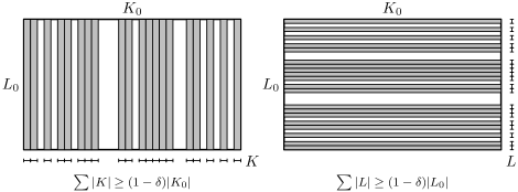
Figure 3. The gray rectangles in the left picture form the collection $\mathscr{K}_{k}(K_{0}\times L_{0})$, the gray rectangles to the right form $\mathscr{L}_{\ell}(K_{0}\times L_{0})$.

Proof.

Define $\mathscr{B}=\{K\times L_{0}:K\subset K_{0}\}\setminus\mathscr{K}(K_{0}\times L_{0})$ and

$$\mathscr{B}_{k}=\mathscr{B}\operatorname{\cap}(\{K\in\mathscr{D}:|K|=2^{-k}|K_{0}|\}\times\mathscr{D}),$$

for all $k\in\mathbb{N}$. Now let

$$A=\bigg{\lfloor}\frac{4}{\rho^{2}\tau^{2}}\bigg{\rfloor}+r.$$

Since each $R\in\mathscr{B}(K_{0}\times L_{0})$ has the form $K\times L_{0}$ for some $K\in\mathscr{D}$, we have

$$\big{\|}\sum_{k=r}^{A}\sum_{R\in\mathscr{B}_{k}}\pm h_{R}\big{\|}_{H^{p}(H^{q})} =\big{\|}\sum_{k=r}^{A}\sum_{K:K\times L_{0}\in\mathscr{B}_{k}}\pm h_{K}\big{\|}_{H^{p}}\|h_{L_{0}}\|_{H^{q}},$$

$$\big{\|}\sum_{k=r}^{A}\sum_{R\in\mathscr{B}_{k}}\pm h_{R}\big{\|}_{H^{p}(H^{q})^{*}} =\big{\|}\sum_{k=r}^{A}\sum_{K:K\times L_{0}\in\mathscr{B}_{k}}\pm h_{K}\big{\|}_{{H^{p}}^{*}}\|h_{L_{0}}\|_{{H^{q}}^{*}}.$$

It is easily verified that $\|h_{L_{0}}\|_{H^{q}}=|L_{0}|^{1/q}$, $\|h_{L_{0}}\|_{{H^{q}}^{*}}=|L_{0}|^{1/q^{\prime}}$, and that

$$\big{\|}\sum_{k=r}^{A}\sum_{K:K\times L_{0}\in\mathscr{B}_{k}}\pm h_{K}\big{\|}_{H^{p}} \leq\sqrt{A-r+1}\,|K_{0}|^{1/p},$$

$$\big{\|}\sum_{k=r}^{A}\sum_{K:K\times L_{0}\in\mathscr{B}_{k}}\pm h_{K}\big{\|}_{{H^{p}}^{*}} \leq\sqrt{A-r+1}\,|K_{0}|^{1/p^{\prime}}.$$

Thus, we note the following estimates

$$\big{\|}\sum_{k=r}^{A}\sum_{R\in\mathscr{B}_{k}}\pm h_{R}\big{\|}_{H^{p}(H^{q})} \leq\sqrt{A-r+1}\,|K_{0}|^{1/p}|L_{0}|^{1/q},$$ (4.6)

$$\big{\|}\sum_{k=r}^{A}\sum_{R\in\mathscr{B}_{k}}\pm h_{R}\big{\|}_{H^{p}(H^{q})^{*}} \leq\sqrt{A-r+1}\,|K_{0}|^{1/p^{\prime}}|L_{0}|^{1/q^{\prime}}.$$

By construction, $\mathscr{B}_{k}$ and $\mathscr{K}_{k}(K_{0}\times L_{0})$ form a disjoint decomposition of $K_{0}\times L_{0}$. We will determine a collection $\mathscr{K}_{k}(K_{0}\times L_{0})$ by showing that $\mathscr{B}_{k}^{*}$ is small enough for at least one value of $k$. Now assume the opposite, namely that

$$|\mathscr{B}_{k}^{*}|\geq\rho|K_{0}\times L_{0}|,\qquad r\leq k\leq A.$$

Summing these estimates yields

$$\sum_{k=r}^{A}|\mathscr{B}_{k}^{*}|\geq(A-r+1)\,\rho\,|K_{0}\times L_{0}|,$$ (4.7)

Observe that by definition of $\mathscr{B}$ and $\mathscr{K}$

$$\tau\cdot\sum_{k=r}^{A}|\mathscr{B}_{k}^{*}|\leq\sum_{j=0}^{i-1}\sum_{k=r}^{A}\sum_{K\times L_{0}\in\mathscr{B}_{k}}|\langle x_{j},h_{K\times L_{0}}\rangle|+|\langle h_{K\times L_{0}},y_{j}\rangle|.$$

Rewriting the right hand side in the following way

$$\sum_{j=0}^{i-1}\Big{|}\Big{\langle}x_{j},\sum_{k=r}^{A}\sum_{K\times L_{0}\in\mathscr{B}_{k}}\pm h_{K\times L_{0}}\Big{\rangle}\Big{|}+\Big{|}\Big{\langle}\sum_{k=r}^{A}\sum_{K\times L_{0}\in\mathscr{B}_{k}}\pm h_{K\times L_{0}},y_{j}\Big{\rangle}\Big{|},$$

and using (4.1) together with (4.6) yields

$$\tau\cdot\sum_{k=r}^{A}|\mathscr{B}_{k}^{*}|\leq 2\sqrt{A-r+1}\,|K_{0}\times L_{0}|.$$

Combining the latter estimate with (4.7), we obtain

$$A\leq\frac{4}{\rho^{2}\tau^{2}}+r-1,$$

which contradicts the definition of $A$. Thus we found $r\leq k\leq A$ so that

$$|\mathscr{K}_{k}^{*}(K_{0}\times L_{0})|\geq(1-\rho)|K_{0}\times L_{0}|,$$

see Figure 3.

The same proof carried out in the other variable can be used the show the estimate for the collections $\mathscr{L}_{\ell}(K_{0}\times L_{0})$. ∎

4.2. Quantitative almost–diagonalization

We show that any given operator on a finite dimensional mixed normed Hardy space or its dual can be almost–diagonalized by a block basis $(b_{R}^{(\varepsilon)})$ of the bi–parameter Haar system. If moreover, the operator has large diagonal with respect to the bi–parameter Haar system, then it has large diagonal with respect to $(b_{R}^{(\varepsilon)})$. The block basis is such that it satisfies the local product conditions (P1)–(P4). We provide quantitative estimates on the number of block basis elements, which depends (among other things) on the dimension of the Hardy space.

Theorem 4.2.

Let $1\leq p,q<\infty$ and $\delta\geq 0$. For $m,n\in\mathbb{N}$ and $\Gamma,\eta>0$ there exists an integer $N=N(m,n,\Gamma,\eta)$ so that the following holds: For any operator $T:H^{p}_{m}(H^{q}_{N})\rightarrow H^{p}_{m}(H^{q}_{N})$ or $T:H^{p}_{m}(H^{q}_{N})^{*}\rightarrow H^{p}_{m}(H^{q}_{N})^{*}$ with $\|T\|\leq\Gamma$ satisfying

$$\langle h_{R},Th_{R}\rangle\geq\delta|R|,\qquad\text{$R\in\mathscr{D}^{m}\times\mathscr{D}^{N}$ },$$ (4.8)

there exists a finite sequence of collections $(\mathscr{B}_{R}:R\in\mathscr{D}^{m}\times\mathscr{D}^{n})$ and a sequence of signs $(\varepsilon_{Q}:Q\in\mathscr{R})$ defining a block basis of the Haar system $b_{R}^{(\varepsilon)}$ by

$$b_{R}^{(\varepsilon)}=\sum_{Q\in\mathscr{B}_{R}}\varepsilon_{Q}h_{Q},\qquad R\in\mathscr{D}^{m}\times\mathscr{D}^{n},$$

so that the following conditions are satisfied:

1. $\mathscr{B}_{R}\subset\mathscr{D}^{m}\times\mathscr{D}^{N}$, for all $R\in\mathscr{D}^{m}\times\mathscr{D}^{n}$.

2. $(\mathscr{B}_{R}:R\in\mathscr{D}^{m}\times\mathscr{D}^{n})$ satisfies local product conditions (P1)–(P4) with constants $C_{X}=1$ and $C_{Y}=1+\eta$.

3. $(b_{R}^{(\varepsilon)}:R\in\mathscr{D}^{m}\times\mathscr{D}^{n})$ almost–diagonalizes $T$ so that $T$ has large diagonal with respect to $(b_{R}^{(\varepsilon)}:R\in\mathscr{D}^{m}\times\mathscr{D}^{n})$. To be more precise, we have the estimates

   $$\sum_{\begin{subarray}{c}R^{\prime}\in\mathscr{D}^{m}\times\mathscr{D}^{n}\\ R^{\prime}\neq R\end{subarray}}|\langle b_{R}^{(\varepsilon)},Tb_{R^{\prime}}^{(\varepsilon)}\rangle| \leq\eta\|b_{R}^{(\varepsilon)}\|_{2}^{2}, R \in\mathscr{D}^{m}\times\mathscr{D}^{n},$$ (4.9a)

   $$\langle b_{R}^{(\varepsilon)},Tb_{R}^{(\varepsilon)}\rangle \geq\delta\|b_{R}^{(\varepsilon)}\|_{2}^{2}, R \in\mathscr{D}^{m}\times\mathscr{D}^{n}.$$ (4.9b)

The proof of Theorem 4.2 relies on a modification of the construction in [7] for the sequence of collections of dyadic rectangles $(\mathscr{B}_{R})$, the combinatorial Lemma 4.1 in $H^{p}(H^{q})$ to make the off–diagonal small, and selecting signs $(\varepsilon_{Q})$ for the block basis $b_{R}^{(\varepsilon)}=\sum_{Q\in\mathscr{B}_{R}}\varepsilon_{Q}h_{Q}$ to keep the diagonal large. See [1] for the one–parameter setting.

Order relation $\operatorname{\vartriangleleft\,}$ on $\mathscr{D}^{m}\times\mathscr{D}^{n}$

The proof of Theorem 4.2 is by induction over the dyadic rectangles $\mathscr{D}^{m}\times\mathscr{D}^{n}$, hence, we need to linearly order them. To this end, let $\operatorname{<_{\ell}}$ denote the lexicographic order on $\mathbb{R}^{4}$. We define the linear order $\operatorname{\vartriangleleft\,}$ on $\mathscr{D}^{m}\times\mathscr{D}^{n}$ by

$$I_{0}\times J_{0}\operatorname{\vartriangleleft\,}I_{1}\times J_{1}\quad\text{if and only if}\quad(|J_{1}|,|I_{1}|,\inf I_{0},\inf J_{0})\operatorname{<_{\ell}}(|J_{0}|,|I_{0}|,\inf I_{1},\inf J_{1}),$$ (4.10)

where $I_{0}\times J_{0},I_{1}\times J_{1}\in\mathscr{D}^{m}\times\mathscr{D}^{n}$. By $\mathcal{O}_{\operatorname{\vartriangleleft\,}}$ we denote the index function given by the following conditions: The function

$$\mathcal{O}_{\operatorname{\vartriangleleft\,}}:\mathscr{D}^{m}\times\mathscr{D}^{n}\to\{k\in\mathbb{Z}:0\leq k<(2^{m+1}-1)(2^{n+1}-1)\}$$

is bijective and satisfies

$$\mathcal{O}_{\operatorname{\vartriangleleft\,}}(R_{0})<\mathcal{O}_{\operatorname{\vartriangleleft\,}}(R_{1})\qquad\text{if and only if}\qquad R_{0}\operatorname{\vartriangleleft\,}R_{1}.$$

See Figure 4.

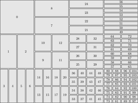
Figure 4. Ordering of the 105 rectangles in $\mathscr{D}^{2}\times\mathscr{D}^{3}$.

Proof of Theorem 4.2.

We only proof the case where $T:H^{p}_{m}(H^{q}_{N})\rightarrow H^{p}_{m}(H^{q}_{N})$. The proof for the case $T:H^{p}_{m}(H^{q}_{N})^{*}\rightarrow H^{p}_{m}(H^{q}_{N})^{*}$ is the same, but the roles of $T$ and $T^{*}$ are reversed.

The proof is separated into the following steps:

• preparation,

• inductive construction of $b_{i_{0}}^{(\varepsilon)}$,

  • construction of $\mathscr{B}_{i_{0}}$,

  • selecting the signs $\varepsilon$,

• verification that $\mathscr{B}_{i_{0}}$ satisfies the local product conditions (P1)–(P4),

• verification that $b_{i_{0}}^{(\varepsilon)}$ almost–diagonalizes $T$.

Preparation

Let $1\leq p,q<\infty$, $\delta\geq 0$, $m,n\in\mathbb{N}$ and $\Gamma,\eta>0$. The number $N=N(m,n,\Gamma,\eta)$ will be determined in the course of the proof. Let $T:H^{p}_{m}(H^{q}_{N})\to H^{p}_{m}(H^{q}_{N})$ be an operator with $\|T\|\leq\Gamma$ such that

$$\langle h_{Q},Th_{Q}\rangle\geq\delta|Q|,\qquad Q\in\mathscr{D}^{m}\times\mathscr{D}^{N}.$$ (4.11)

Given $Q\in\mathscr{D}^{m}\times\mathscr{D}^{N}$ we write

$$Th_{Q}=\alpha_{Q}h_{Q}+r_{Q},$$ (4.12a)

where

$$\alpha_{Q}=\frac{\langle h_{Q},Th_{Q}\rangle}{|Q|}\qquad\text{and}\qquad r_{Q}=\sum_{Q^{\prime}:Q^{\prime}\neq Q}\frac{\langle h_{Q^{\prime}},Th_{Q}\rangle}{|Q^{\prime}|}h_{Q^{\prime}}.$$ (4.12b)

Note that for all $Q=K\times L\in\mathscr{D}^{m}\times\mathscr{D}^{N}$ we have the estimates

$$\delta\leq\alpha_{Q}\leq\|T\|\qquad\text{and}\qquad\|r_{Q}\|_{H^{p}(H^{q})}\leq 2\|T\||K|^{1/p}|L|^{1/q}.$$ (4.13)

Inductive construction of $(b_{R}^{(\varepsilon)}:R\in\boldsymbol{\mathscr{D}}^{m}\times\boldsymbol{\mathscr{D}}^{n})$

For fixed $R\in\mathscr{D}^{m}\times\mathscr{D}^{n}$, the block basis element $b_{R}^{(\varepsilon)}$ will be determined by a collection of dyadic rectangles $\mathscr{B}_{R}\subset\mathscr{D}^{m}\times\mathscr{D}^{N}$ and signs $\varepsilon=(\varepsilon_{Q}:Q\in\mathscr{D}^{m}\times\mathscr{D}^{N})$, and is of the following form:

$$b_{R}^{(\varepsilon)}=\sum_{Q\in\mathscr{B}_{R}}\varepsilon_{Q}h_{Q}.$$ (4.14)

From now on, we sytematically use the following rule: whenever $\mathcal{O}_{\operatorname{\vartriangleleft\,}}(R)=i$, we set

$$\mathscr{B}_{i}=\mathscr{B}_{R}\qquad\text{and}\qquad b_{i}^{(\varepsilon)}=b_{R}^{(\varepsilon)}.$$

In the course of this proof we will construct the finite sequence of collections $(\mathscr{B}_{R}:R\in\mathscr{D}^{m}\times\mathscr{D}^{n})$ and signs $\varepsilon=(\varepsilon_{Q}:Q\in\mathscr{D}^{m}\times\mathscr{D}^{N})$ so that $(\mathscr{B}_{R}:R\in\mathscr{D}^{m}\times\mathscr{D}^{n})$ satisfies the local product conditions (P1)–(P4) with constants $C_{X}=1$ and $C_{Y}=1+\eta$, and that the block basis $(b_{i}^{(\varepsilon)})_{i\in\mathbb{N}_{0}}$ given by (4.14) satisfies

$$\sum_{j=0}^{i-1}|\langle T^{*}b_{j}^{(\varepsilon)},b_{i}^{(\varepsilon)}\rangle|+|\langle b_{i}^{(\varepsilon)},Tb_{j}^{(\varepsilon)}\rangle| \leq c(\eta^{\prime})4^{-i-1}\|b_{i}^{(\varepsilon)}\|_{2}^{2},$$ (4.15a)

$$\langle b_{i}^{(\varepsilon)},Tb_{i}^{(\varepsilon)}\rangle \geq\delta\|b_{i}^{(\varepsilon)}\|_{2}^{2},$$ (4.15b)

for all $i\in\mathbb{N}_{0}$, where $c(\eta^{\prime})\to 0$ as $\eta^{\prime}\to 0$. We now choose $\eta^{\prime}=\eta^{\prime}(m,n,\Gamma,\eta)>0$ so small that

$$(1-\eta^{\prime})^{-1}\leq 1+\eta\qquad\text{and}\qquad\eta^{\prime}(1-\eta^{\prime})^{-2}4^{m+n}\Gamma\leq\eta.$$ (4.16)

The induction begins by putting

$$\mathscr{B}_{0}=\{[0,1)\times[0,1)\}\qquad\text{and}\qquad b_{0}^{(\varepsilon)}=h_{[0,1)\times[0,1)}.$$ (4.17)

Let $i_{0}\in\mathbb{N}$. At this stage we assume:

• There exist collections $\mathscr{B}_{j}=\mathscr{B}_{I\times J}$, for all $\mathcal{O}_{\operatorname{\vartriangleleft\,}}(I\times J)=j\leq i_{0}-1$ of the the form

  $$\mathscr{B}_{I\times J}=\big{\{}I\times L:L\in\mathscr{Y}_{I\times J}\big{\}},$$

  where $\mathscr{Y}_{I\times J}$ is a finite subset of $\mathscr{D}$. In the notation of Section 3, $\mathscr{X}_{I\times J}=\{I\}$.

• The collections $\mathscr{B}_{j}$, $0\leq j\leq i_{0}-1$, are such that $(\mathscr{B}_{j})_{j=0}^{i_{0}-1}$ satisfies the local product conditions (P1)–(P4).

• The block basis elements $b_{j}^{(\varepsilon)}$, given by (4.14), satisfy (4.15) for $0\leq j\leq i_{0}-1$.

Now, we turn to the construction of $\mathscr{B}_{i_{0}}$ and $\varepsilon_{Q}$, where $Q\in\mathscr{B}_{i_{0}}$. In the first step we find $\mathscr{B}_{i_{0}}$, and only then we will determine the signs $\varepsilon$.

Construction of $\boldsymbol{\mathscr{B}}\bm{{}_{i_{0}}}$

Let $I_{0}\times J_{0}\in\mathscr{R}$ such that $\mathcal{O}_{\operatorname{\vartriangleleft\,}}(I_{0}\times J_{0})=i_{0}$. At the beginning of the construction as well as at the end, we will distinguish between the two cases

$$I_{0}\neq[0,1)\qquad\text{and}\qquad I_{0}=[0,1).$$

In both cases, we will use the combinatorial Lemma 4.1.

If $I_{0}\neq[0,1)$ we define the collection $\mathscr{P}_{I_{0}\times J_{0}}$ by

$$\mathscr{P}_{I_{0}\times J_{0}}=\{I\times J\in\mathscr{D}^{m}\times\mathscr{D}^{n}:I\times J\operatorname{\vartriangleleft\,}I_{0}\times J_{0},I\neq I_{0}\},$$ (4.18a)

and if $$I_{0}=[0,1)$$, we put

$$\mathscr{P}_{[0,1)\times J_{0}}=\{I\times J\in\mathscr{D}^{m}\times\mathscr{D}^{n}:I\times J\operatorname{\vartriangleleft\,}[0,1)\times J_{0},|J|>|J_{0}|\}.$$ (4.18b)

In both cases, we now define $\mathbb{A}_{I_{0}\times J_{0}}$ by

$$\mathbb{A}_{I_{0}\times J_{0}}=\big{\{}\{I\times J^{\prime}\in\mathscr{P}_{I_{0}\times J_{0}}:|J^{\prime}|=|J|\}:I\times J\in\mathscr{P}_{I_{0}\times J_{0}}\big{\}}.$$ (4.19)

Before we proceed with the proof, we make a few remarks.

• For all $J\in\mathscr{D}^{n}$ with $|J|=|J_{0}|$ holds that $\mathscr{P}_{I_{0}\times J}=\mathscr{P}_{I_{0}\times J_{0}}$, and hence $\mathbb{A}_{I_{0}\times J}=\mathbb{A}_{I_{0}\times J_{0}}$.

• If $I\times J\in\mathscr{A}\in\mathbb{A}_{I_{0}\times J_{0}}$, then

  $$\mathscr{A}=\{I\times J^{\prime}:J^{\prime}\in\mathscr{D},\ |J^{\prime}|=|J|\}$$ (4.20)

  see (4.10) and (4.19).

• The collection $\mathbb{A}_{I_{0}\times J_{0}}$ is a partition of $\mathscr{P}_{I_{0}\times J_{0}}$, i.e.

  $$\bigcup\mathbb{A}_{I_{0}\times J_{0}}=\mathscr{P}_{I_{0}\times J_{0}}\qquad\text{and}\qquad\mathscr{A}\cap\mathscr{A}^{\prime}=\emptyset$$

  for all $\mathscr{A},\mathscr{A}^{\prime}\in\mathbb{A}_{I_{0}\times J_{0}}$ with $\mathscr{A}\neq\mathscr{A}^{\prime}$.

• The collections $\mathscr{Y}_{I\times J}$ have already been constructed for all $I\times J\in\mathscr{P}_{I_{0}\times J_{0}}$.

• Let $\mathscr{A}\in\mathbb{A}_{I_{0}\times J_{0}}$ and $I\times J,I\times J^{\prime}\in\mathscr{A}$, then

  $$Y_{I\times J}\cap Y_{I\times J^{\prime}}=\emptyset,\qquad\text{if $J\neq J^{\prime}$}.$$

For each $\mathscr{A}\in\mathbb{A}_{I_{0}\times J_{0}}$, let $W(\mathscr{A})$ denote the set given by

$$W(\mathscr{A})=\bigcup_{I\times J\in\mathscr{A}}Y_{I\times J}.$$ (4.21)

Note that for each $\mathscr{A}\in\mathbb{A}_{I_{0}\times J_{0}}$ the set $W(\mathscr{A})$ is an almost cover of the unit interval. Now we define $W_{I_{0}\times J_{0}}$ by intersecting all the $W(\mathscr{A})$:

$$W_{I_{0}\times J_{0}}=\bigcap_{\mathscr{A}\in\mathbb{A}_{I_{0}\times J_{0}}}W(\mathscr{A}).$$ (4.22)

We will cover the set $W_{I_{0}\times J_{0}}$ with smaller intervals than we have previously used in our construction. To this end let

$$\gamma_{i_{0}}=\gamma_{I_{0}\times J_{0}}=\frac{1}{2}\min\{|L|:\exists I\times J\operatorname{\vartriangleleft\,}I_{0}\times J_{0},\ \mathscr{Y}_{I\times J}\ni L\}$$ (4.23)

and define the high frequency cover $\mathscr{W}_{I_{0}\times J_{0}}$ of $W_{I_{0}\times J_{0}}$ by

$$\mathscr{W}_{I_{0}\times J_{0}}=\{L_{0}\in\mathscr{D}:|L_{0}|=\gamma_{I_{0}\times J_{0}},\ L_{0}\subset W_{I_{0}\times J_{0}}\}.$$ (4.24)

Note the following identity:

$$\operatorname*{\bigcup}\mathscr{W}_{I_{0}\times J_{0}}=W_{I_{0}\times J_{0}}.$$ (4.25)

To each of the rectangles $I_{0}\times L_{0}$, where $L_{0}\in\mathscr{W}_{I_{0}\times J_{0}}$, we will now prepare to apply Lemma 4.1, so that $I_{0}$ will remain intact, and $L_{0}$ will be almost covered with high frequencies $L$. To this end let

$$\beta_{i_{0}}=\beta_{I_{0}\times J_{0}}=\min\{|I_{0}\times L_{0}|:L_{0}\in\mathscr{W}_{I_{0}\times J_{0}}\}$$ (4.26)

and define for all $0\leq j\leq i_{0}-1$

$$x_{j} :=\frac{\beta_{i_{0}}}{\Gamma i_{0}\|b_{j}^{(\varepsilon)}\|_{H^{p}(H^{q})^{*}}}T^{*}b_{j}^{(\varepsilon)}, y_{j} :=\frac{\beta_{i_{0}}}{\Gamma i_{0}\|b_{j}^{(\varepsilon)}\|_{H^{p}(H^{q})}}Tb_{j}^{(\varepsilon)}.$$ (4.27)

Recall that $\|T\|\leq\Gamma$, hence

$$\sum_{j=0}^{i_{0}-1}\|x_{j}\|_{H^{p}(H^{q})^{*}}\leq\beta_{i_{0}}\qquad\text{and}\qquad\sum_{j=0}^{i_{0}-1}\|y_{j}\|_{{}_{H^{p}(H^{q})}}\leq\beta_{i_{0}}.$$

The local frequency weight $f_{i_{0}}$ is given by

$$f_{i_{0}}(Q)=\sum_{j=0}^{i_{0}-1}|\langle x_{j},h_{Q}\rangle|+|\langle y_{j},h_{Q}\rangle|,\qquad Q\in\mathscr{R},$$ (4.28)

and the constant $\tau_{i_{0}}$ by

$$\tau_{i_{0}}=\tau_{I_{0}\times J_{0}}=\frac{\eta^{\prime}\beta_{i_{0}}}{i_{0}4^{i_{0}+1}}.$$ (4.29)

For each $L_{0}\in\mathscr{W}_{I_{0}\times J_{0}}$ we put

$$\mathscr{L}(I_{0}\times L_{0})=\{I_{0}\times L:L\in\mathscr{D},\ L\subsetneq L_{0},\ f_{i_{0}}(I_{0}\times L)\leq\tau_{i_{0}}|I_{0}\times L|\}.$$ (4.30)

Finally, we define the constant $\rho_{i_{0}}$ by

$$\rho_{i_{0}}=\rho_{I_{0}\times J_{0}}=\frac{\eta^{\prime}}{4^{i_{0}}}.$$ (4.31)

Since $\beta_{i_{0}}\leq|I_{0}|^{1/{p^{\prime}}}|L_{0}|^{1/{q^{\prime}}}$ and $\beta_{i_{0}}\leq|I_{0}|^{1/p}|L_{0}|^{1/q}$, for all $L_{0}\in\mathscr{W}_{I_{0}\times J_{0}}$, Lemma 4.1 yields an integer $\ell=\ell(I_{0}\times L_{0})$ with

$$1\leq\ell\leq\bigg{\lfloor}\frac{4}{\rho_{i_{0}}^{2}\tau_{i_{0}}^{2}}\bigg{\rfloor}+1,$$ (4.32)

such that the collection $\mathscr{L}_{\ell}(I_{0}\times L_{0})$ given by

$$\mathscr{L}_{\ell}(I_{0}\times L_{0})=\{I_{0}\times L\in\mathscr{L}(I_{0}\times L_{0}):|L|=2^{-\ell}|L_{0}|\}$$

satisfies the estimate

$$(1-\rho_{i_{0}})|I_{0}\times L_{0}|\leq\Big{|}\bigcup\{Q:Q\in\mathscr{L}_{\ell}(I_{0}\times L_{0})\}\Big{|}\leq|I_{0}\times L_{0}|.$$

Now, we take the union over all $L_{0}\in\mathscr{W}_{I_{0}\times J_{0}}$ to obtain

$$\mathscr{Z}_{I_{0}\times J_{0}}=\operatorname*{\bigcup}\big{\{}\mathscr{L}_{\ell}(I_{0}\times L_{0}):L_{0}\in\mathscr{W}_{I_{0}\times J_{0}}\big{\}}.$$ (4.33)

Once again, we emphasize that $\ell=\ell(I_{0}\times L_{0})$ in the above formula. Let $Z_{I_{0}\times J_{0}}$ denote the pointset of $\mathscr{Z}_{I_{0}\times J_{0}}$, i.e.

$$Z_{I_{0}\times J_{0}}=\bigcup\mathscr{Z}_{I_{0}\times J_{0}},$$

then for all $L_{0}\in\mathscr{W}_{I_{0}\times J_{0}}$ we have the estimates

$$(1-\rho_{i_{0}})|I_{0}\times L_{0}|\leq\Big{|}Z_{I_{0}\times J_{0}}\cap(I_{0}\times L_{0})\Big{|}\leq|I_{0}\times L_{0}|.$$ (4.34)

We want to point out that $Q\in\mathscr{Z}_{I_{0}\times J_{0}}$ implies $Q=I_{0}\times L$, for some $L\in\mathscr{D}$. There exists a unique $L_{0}\in\mathscr{W}_{I_{0}\times J_{0}}$ such that $L_{0}\supset L$, and therefore $|L|=2^{-\ell}$, where $\ell=\ell(I_{0}\times L_{0})$.

Case 1: $I_{0}\neq[0,1)$.

Here, we know that $2^{-m}\leq|I_{0}|\leq 1/2$. Let $\widetilde{I}_{0}$ be the dyadic predecessor of $I_{0}$, then $\mathscr{B}_{\widetilde{I}_{0}\times J_{0}}$ has already been defined (see (4.10)). The block basis indexed by the dark gray rectangles has already been constructed. Here, we determine the block basis for the light gray rectangles. The white ones will be treated later.

In this case we put

$$\mathscr{B}_{I_{0}\times J_{0}}=\{I_{0}\times L\in\mathscr{Z}_{I_{0}\times J_{0}}:I_{0}\times L\subset B_{\widetilde{I}_{0}\times J_{0}}\}.$$ (4.35)

see Figure 5.

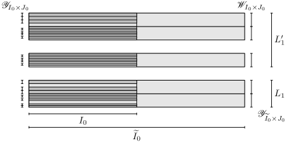
Figure 5. In this figure, the dyadic interval $I_{0}$ is the left half of $\widetilde{I}_{0}$, and the collection $\mathscr{Y}_{\widetilde{I}_{0}\times J_{0}}$ consists of the dyadic intervals $L_{1}$ and $L_{1}^{\prime}$. Immediately to the left of $L_{1}$, $L_{1}^{\prime}$ are the unlabeled dyadic intervals of the collection $\mathscr{W}_{I_{0}\times J_{0}}$. Note that all the intervals in $\mathscr{W}_{I_{0}\times J_{0}}$ have the same length, see (4.24). The pointset $W_{I_{0}\times J_{0}}$ of $\mathscr{W}_{I_{0}\times J_{0}}$ almost covers each of the intervals $L_{1}$, $L_{1}^{\prime}$, see (4.19), (4.20), (4.21), (4.22) and (4.25). The light gray rectangles are formed by the product of $\widetilde{I}_{0}$ with the intervals in $\mathscr{W}_{I_{0}\times J_{0}}$. The collection of dyadic intervals $\mathscr{Y}_{I_{0}\times J_{0}}$ is given by the unlabeled vertical intervals to the very left of the figure are determined by the combinatorial Lemma 4.1. The pointset $Y_{I_{0}\times J_{0}}$ of $\mathscr{Y}_{I_{0}\times J_{0}}$ almost covers each interval in $\mathscr{W}_{I_{0}\times J_{0}}$, and therefore each interval in $\mathscr{Y}_{\widetilde{I}_{0}\times J_{0}}=\{L_{1},L_{1}^{\prime}\}$, see (4.30), (4.33) (4.34) and (4.35). The collection $\mathscr{B}_{I_{0}\times J_{0}}$ consists of the dark gray rectangles and is given by $\{I_{0}\times L:L\in\mathscr{Y}_{I_{0}\times J_{0}}\}$.

By (4.35) we obtain that

$$K\times L\in\mathscr{B}_{I_{0}\times J_{0}}\quad\text{implies}\quad K=I_{0},$$ (4.36)

thus, (4.34), (4.35) and (4.36) yield

$$\mathscr{X}_{I_{0}\times J_{0}}=\{I_{0}\}$$ (4.37a)

and

$$(1-\rho_{I_{0}\times J_{0}})|L|\leq|Y_{I_{0}\times J_{0}}\cap L|\leq|L|,$$ (4.37b)

for all $L\in\mathscr{Y}_{I\times J}$ with $L\cap Y_{I_{0}\times J_{0}}\neq\emptyset$, where $I\times J\in\mathscr{P}_{I_{0}\times J_{0}}$ is maximal with respect to the ordering $\operatorname{\vartriangleleft\,}$ (in which case $I\neq I_{0}$, $J=J_{0}$ and we have $L\cap Y_{I_{0}\times J_{0}}\neq\emptyset$ for all $L\in\mathscr{Y}_{I\times J}$).

Case 2: $I_{0}=[0,1)$

In this case we know that $\mathscr{B}_{I\times\widetilde{J}_{0}}$ has already been constructed for all $I\in\mathscr{D}^{m}$ (see (4.10)); those are the dark gray rectangles in the third column. Here, we determine the block basis for the light gray rectangles. The white ones will be treated later.

Here, we define the sets

$$B_{[0,1)\times\widetilde{J}_{0}}^{\ell}=\operatorname*{\bigcup}_{[0,1)\times L_{0}\in\mathscr{B}_{[0,1)\times\widetilde{J}_{0}}}[0,1)\times L_{0}^{\ell}$$

and

$$B_{[0,1)\times\widetilde{J}_{0}}^{r}=\operatorname*{\bigcup}_{[0,1)\times L_{0}\in\mathscr{B}_{[0,1)\times\widetilde{J}_{0}}}[0,1)\times L_{0}^{r}.$$

If $$J_{0} \widetilde{J}_{0}$$ is the left half of we put

$$\mathscr{B}_{[0,1)\times J_{0}}=\{[0,1)\times L\in\mathscr{Z}_{[0,1)\times J_{0}}:[0,1)\times L\subset B_{[0,1)\times\widetilde{J}_{0}}^{\ell}\}.$$ (4.38a)

If $$J_{0} \widetilde{J}_{0}$$ is the right half of we put

$$\mathscr{B}_{[0,1)\times J_{0}}=\{[0,1)\times L\in\mathscr{Z}_{[0,1)\times J_{0}}:[0,1)\times L\subset B_{[0,1)\times\widetilde{J}_{0}}^{r}\},$$ (4.38b)

see Figure 6.

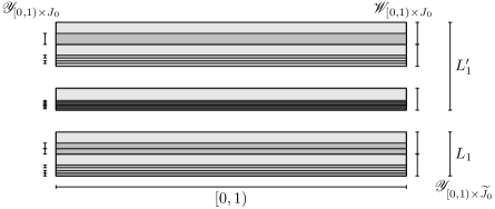
Figure 6. In this figure, $J_{0}$ is the left half of $\widetilde{J}_{0}$. The collection of dyadic intervals $\mathscr{Y}_{[0,1)\times\widetilde{J}_{0}}=\{L_{1},L_{1}^{\prime}\}$ are the $y$–components of the collection $\mathscr{B}_{[0,1)\times\widetilde{J}_{0}}$. To the left is the collection $\mathscr{W}_{[0,1)\times J_{0}}$, whose pointset $W_{[0,1)\times J_{0}}$ almost covers $L_{1}$ and $L_{1}^{\prime}$. The light gray dyadic rectangles are determined by the products $[0,1)\times L_{0}$, where $L_{0}\in\mathscr{W}_{[0,1)\times J_{0}}$. The dark gray rectangles are the output of the combinatorial Lemma 4.1, and are all contained in the left halves in one of the intervals $L_{0}\in\mathscr{W}_{[0,1)\times J_{0}}$ (since $J_{0}$ is the left half of $\widetilde{J}_{0}$, see (4.38)). The dark gray rectangles form the collection $\mathscr{B}_{[0,1)\times J_{0}}$. The collection $\mathscr{Y}_{[0,1)\times J_{0}}$ is the collection of $y$–components of $\mathscr{B}_{[0,1)\times J_{0}}$.

In this case, we have by (4.38) that

$$K\times L\in\mathscr{B}_{[0,1)\times J_{0}}\quad\text{implies}\quad K=[0,1),$$ (4.39)

thus, (4.34), (4.38) and (4.39) yield

$$\mathscr{X}_{[0,1)\times J_{0}}=\{[0,1)\}$$ (4.40a)

and

$$\frac{1}{2}(1-2\rho_{[0,1)\times J_{0}})|L|\leq|Y_{[0,1)\times J_{0}}\cap L|\leq|L|,$$ (4.40b)

for all $L\in\mathscr{Y}_{I\times J}$ with $L\cap Y_{I_{0}\times J_{0}}\neq\emptyset$, where $I\times J\in\mathscr{P}_{I_{0}\times J_{0}}$ is maximal with respect to the ordering $\operatorname{\vartriangleleft\,}$ (in which case $I=[1-2^{-m},1)$, $J=\widetilde{J}_{0}$ and $L\cap Y_{I_{0}\times J_{0}}\neq\emptyset$ for all $L\in\mathscr{Y}_{I\times J}$).

Recall that $i_{0}=\mathcal{O}_{\operatorname{\vartriangleleft\,}}(I_{0}\times J_{0})$, and that $\mathscr{B}_{i_{0}}=\mathscr{B}_{I_{0}\times J_{0}}$ as well as $b_{i_{0}}^{(\varepsilon)}=b_{I_{0}\times J_{0}}^{(\varepsilon)}$. By the definition of $\mathscr{L}(I_{0}\times L_{0})$ (see (4.30)) and the definition of $\mathscr{B}_{i_{0}}$ (see (4.35) and (4.38)), we note that in both cases

$$f_{i_{0}}(Q)\leq\tau_{i_{0}}|Q|,\qquad Q\in\mathscr{B}_{i_{0}}.$$ (4.41)

Selecting the signs $\bm{\varepsilon}$

In any of the above cases (4.35) and (4.38), we define the following function. For any choice of signs $\varepsilon_{Q}\in\{-1,+1\}$, $Q\in\mathscr{B}_{i_{0}}$ put

$$b_{i_{0}}^{(\varepsilon)}=\sum_{Q\in\mathscr{B}_{i_{0}}}\varepsilon_{Q}h_{Q}.$$ (4.42)

We will now select signs $(\varepsilon_{Q}:Q\in\mathscr{B}_{i_{0}})$ such that

$$\langle b_{i_{0}}^{(\varepsilon)},Tb_{i_{0}}^{(\varepsilon)}\rangle\geq\delta\|b_{i_{0}}^{(\varepsilon)}\|_{2}^{2}.$$

To this end observe that (4.12) and (4.42) yields

$$\langle b_{i_{0}}^{(\varepsilon)},Tb_{i_{0}}^{(\varepsilon)}\rangle=\sum_{Q\in\mathscr{B}_{i_{0}}}\alpha_{Q}|Q|+\langle b_{i_{0}}^{(\varepsilon)},R_{m}^{(\varepsilon)}\rangle,$$

where

$$R_{m}^{(\varepsilon)}=\sum_{Q\in\mathscr{B}_{i_{0}}}\varepsilon_{Q}r_{Q}.$$

Thus, by (4.13) we get

$$\langle b_{i_{0}}^{(\varepsilon)},Tb_{i_{0}}^{(\varepsilon)}\rangle\geq\delta\|b_{i_{0}}^{(\varepsilon)}\|_{2}^{2}+\langle b_{i_{0}}^{(\varepsilon)},R_{m}^{(\varepsilon)}\rangle,$$

Let $\operatorname{\mathbb{E}}_{\varepsilon}$ denote the average over all possible choices of signs $(\varepsilon_{Q}:Q\in\mathscr{B}_{i_{0}})$. Using $\langle h_{Q},r_{Q}\rangle=0$, we obtain

$$\langle b_{i_{0}}^{(\varepsilon)},R_{m}^{(\varepsilon)}\rangle=\sum\varepsilon_{Q_{0}}\varepsilon_{Q_{1}}\langle h_{Q_{0}},r_{Q_{1}}\rangle,$$

where the sum is taken over all $Q_{0},Q_{1}\in\mathscr{B}_{i_{0}}$ with $Q_{0}\neq Q_{1}$. Taking the expectation on the right hand side we obtain,

$$\operatorname{\mathbb{E}}_{\varepsilon}\langle b_{i_{0}}^{(\varepsilon)},R_{m}^{(\varepsilon)}\rangle=0.$$

This gives

$$\operatorname{\mathbb{E}}_{\varepsilon}\langle b_{i_{0}}^{(\varepsilon)},Tb_{i_{0}}^{(\varepsilon)}\rangle\geq\delta\operatorname{\mathbb{E}}_{\varepsilon}\|b_{i_{0}}^{(\varepsilon)}\|_{2}^{2},$$ (4.43)

hence there exists at least one $\varepsilon$ such that

$$\langle b_{i_{0}}^{(\varepsilon)},Tb_{i_{0}}^{(\varepsilon)}\rangle\geq\delta\|b_{i_{0}}^{(\varepsilon)}\|_{2}^{2}.$$ (4.44)

$(\boldsymbol{\mathscr{B}}\bm{{}_{i}:i\leq i_{0}})$ satisfies the local product conditions (P1)–(P4).

It should be clear from the definition of $\mathscr{F}_{m}$ in each step, that $(\mathscr{B}_{i}:i\leq i_{0})$ satisfies (P1). Since $\mathscr{X}_{I\times J}=\{I\}$ for all $I\times J\in\mathscr{D}^{m}\times\mathscr{D}^{n}$, (P2)–(P4) is satisfied with $C_{X}=1$. Recalling the definition of $Y_{J}$ (see (3.4)), and that the new $y$–components are obtained by intersecting all the supports from the previous steps (see (4.21), (4.22), (4.24), (4.25), (4.30), (4.33), (4.35), and (4.38)) we observe that

$$Y_{J}=\bigcup_{I\in\mathscr{D}^{m}}Y_{I\times J}=Y_{[0,1)\times J},\qquad J\in\mathscr{D}^{n}.$$

By considering (4.38) together with the above identity, it should be clear that $(Y_{J}:J\in\mathscr{D}^{n})$ satisfies (P2) and $|Y_{J}|\leq|J|$, $J\in\mathscr{D}^{n}$. The remaining measure estimates (P3) and (P4) follow by induction from (4.37) and (4.40).

Now, let $I_{0}\times J_{0},I\times J\in\mathscr{D}^{m}\times\mathscr{D}^{n}$ with $I_{0}\times J_{0}\subsetneq I\times J$ and let $L\in\mathscr{Y}_{I\times J}$. From (4.37) and (4.40) follows immediately that $K_{0}=I_{0}$ and $K=I$. Since the $\rho_{i}$ are a geometric sequence (see (4.31)), we obtain by induction that

$$\frac{|J_{0}|}{|J|}(1-\eta^{\prime})|L|\leq|L\cap Y_{I_{0}\times J_{0}}|\leq\frac{|J_{0}|}{|J|}|L|.$$ (4.45)

We remark that (4.45) implies (P3) and (P4) with $C_{Y}=C_{Y}(\eta^{\prime})=(1-\eta^{\prime})^{-1}$. To summarize, we showed that $(\mathscr{B}_{R}:R\in\mathscr{D}^{m}\times\mathscr{D}^{n})$ satisfies the local product conditions (P1)–(P4) with constants $C_{X}=1$ and $C_{Y}=(1-\eta^{\prime})^{-1}$.

The block basis $\bm{(b_{i}^{(\varepsilon)}:i\leq i_{0})}$ almost–diagonalizes $\bm{T}$.

First, recall that the constant $\tau_{i}$ was given by $\tau_{i}=\frac{\eta^{\prime}\beta_{i}}{i4^{i+1}}$ (see (4.26) and (4.29)). With that in mind, we collect the estimates (4.41), (see (4.28) for the definition of $f_{i_{0}}$) and the mixed norm estimates in Theorem 3.1 to obtain

$$\sum_{j=0}^{i-1}|\langle T^{*}b_{j}^{(\varepsilon)},h_{Q}\rangle|+|\langle h_{Q},Tb_{j}^{(\varepsilon)}\rangle|\leq\eta^{\prime}(1-\eta^{\prime})^{-1}2^{m+n}\Gamma 4^{-i-1}|Q|,$$

for all $i$ and $Q\in\mathscr{B}_{i}$. From the latter estimate and the definition of $b_{i}^{(\varepsilon)}$ (see (4.42)) we obtain by summing over $Q\in\mathscr{B}_{i}$

$$\sum_{j=0}^{i-1}|\langle T^{*}b_{j}^{(\varepsilon)},b_{i}^{(\varepsilon)}\rangle|+|\langle b_{i}^{(\varepsilon)},Tb_{j}^{(\varepsilon)}\rangle|\leq\eta^{\prime}(1-\eta^{\prime})^{-1}2^{m+n}\Gamma 4^{-i-1},\qquad i\geq 1.$$ (4.46)

From the first term in the sum of (4.46) follows the estimate

$$|\langle b_{i}^{(\varepsilon)},Tb_{j}^{(\varepsilon)}\rangle|\leq\eta^{\prime}(1-\eta^{\prime})^{-1}2^{m+n}\Gamma 4^{-j-1},\qquad j>i\geq 0.$$

Summing over all those $j$ we obtain

$$\sum_{j\geq i+1}|\langle b_{i}^{(\varepsilon)},Tb_{j}^{(\varepsilon)}\rangle|\leq\eta^{\prime}(1-\eta^{\prime})^{-1}2^{m+n}\Gamma 4^{-i-1},\qquad i\geq 0.$$

Combining the latter estimate with (4.46) and using that $\|b_{i}\|_{2}^{2}\geq(1-\eta^{\prime})2^{-m-n}$ (see (3.7) and recall that $b_{i}=b_{R}$, whenever $i=\mathcal{O}_{\operatorname{\vartriangleleft\,}}(R)$, and that here $R\in\mathscr{D}^{m}\times\mathscr{D}^{n}$) yields

$$\sum_{\begin{subarray}{c}j:j\neq i\end{subarray}}|\langle b_{i}^{(\varepsilon)},Tb_{j}^{(\varepsilon)}\rangle|\leq\eta^{\prime}(1-\eta^{\prime})^{-2}4^{m+n}\Gamma\|b_{i}^{(\varepsilon)}\|_{2}^{2},\qquad i\geq 0.$$ (4.47)

We remark that (4.47) and (4.16) together with (4.44) proves (4.9).

Finally, observe that (i) of Theorem 4.2 holds true by observing that all the constants in the proof depend only on $m,n,\Gamma$ and $\eta$ (see (4.16), (4.23), (4.26), (4.29), (4.30), (4.31) and (4.32)). ∎

Remark 4.3.

Let $(e_{K})$ and $(f_{L})$ denote block bases of the one parameter Haar system satisfying the hypothesis of the reiteration Lemma 3.2, that is $(e_{K}\otimes f_{L})$ satisfies the local product conditions (P1)–(P4), and additional regularity assumptions (see Lemma 3.2 (i) and (ii)).

We remark that we could repeat the proof of Theorem 4.2 with $h_{K\times L}$ replaced by $\widetilde{h}_{K\times L}=e_{K}\otimes f_{L}$, $K\times L\in\mathscr{D}^{m}\times\mathscr{D}^{N}$. Due to the reiteration Lemma 3.2, we would arrive at the same conclusion. To be more precise: if we replace (4.8) in Theorem 4.2 by

$$\langle\widetilde{h}_{Q},T\widetilde{h}_{Q}\rangle\geq\delta\|\widetilde{h}_{Q}\|_{2}^{2},\qquad Q\in\mathscr{D}^{m}\times\mathscr{D}^{N},$$ (4.48)

then all the conclusions (i)–(4.9) of Theorem 4.2 remain valid for the block basis $(\widetilde{b}_{R}^{(\varepsilon)}:R\in\mathscr{D}^{m}\times\mathscr{D}^{n})$ of the bi–parameter Haar system given by

$$\widetilde{b}_{R}^{(\varepsilon)}=\sum_{Q\in\mathscr{B}_{R}}\varepsilon_{Q}\widetilde{h}_{Q},\qquad R\in\mathscr{D}^{m}\times\mathscr{D}^{n}.$$

4.3. Projections that almost annihilate finite dimensional subspaces

In the proof of the main result Theorem 2.1, we will use the almost–diagonalization result Theorem 4.2. Additionally, we will need the following variation of Theorem 4.2.

Theorem 4.4.

Let $1\leq p,q<\infty$, $m,n,d\in\mathbb{N}$ and $\eta>0$. Then there exists an integer $N=N(m,n,d,\eta)$ so that for any $d$–dimensional subspace $F\subset H_{m}^{p}(H_{N}^{q})$ (respectively $F\subset H_{m}^{p}(H_{N}^{q})^{*}$) there exists a block basis $(b_{R}:R\in\mathscr{D}^{m}\times\mathscr{D}^{n})$ satisfying the following conditions:

1. $\mathscr{B}_{R}\subset\mathscr{D}^{m}\times\mathscr{D}^{N}$, for all $R\in\mathscr{D}^{m}\times\mathscr{D}^{n}$.

2. For every finite sequence of scalars $(a_{R}:R\in\mathscr{D}^{m}\times\mathscr{D}^{n})$ we have that

   $$(1+\eta)^{-1}\Big{\|}\sum_{R\in\mathscr{D}^{m}\times\mathscr{D}^{n}}a_{R}h_{R}\Big{\|}\leq\Big{\|}\sum_{R\in\mathscr{D}^{m}\times\mathscr{D}^{n}}a_{R}b_{R}\Big{\|}\leq(1+\eta)\Big{\|}\sum_{R\in\mathscr{D}^{m}\times\mathscr{D}^{n}}a_{R}h_{R}\Big{\|}.$$ (4.49)

   The above norms are either all the norm of $H^{p}(H^{q})$, or they are all the norm of $H^{p}(H^{q})^{*}$.

3. The orthogonal projection $Q:H_{m}^{p}(H_{N}^{q})\rightarrow H_{m}^{p}(H_{N}^{q})$ (respectively $Q:H_{m}^{p}(H_{N}^{q})^{*}\rightarrow H_{m}^{p}(H_{N}^{q})^{*}$) given by

   $$Qf=\sum_{R\in\mathscr{D}^{m}\times\mathscr{D}^{n}}\frac{\langle f,b_{R}\rangle}{\|b_{R}\|_{2}^{2}}\,b_{R}$$

   satisfies the estimates

   $$\|Qf\| \leq(1+\eta)\|f\|, f \in H_{m}^{p}(H_{N}^{q})\ \text{(respectively $f\in H_{m}^{p}(H_{N}^{q})^{*}$)},$$ (4.50)

   $$\|Qf\| \leq\eta\,\|f\|, f \in F.$$

   The above norms are either all the norm of $H^{p}(H^{q})$, or they are all the norm of $H^{p}(H^{q})^{*}$.

Proof.

The proof of Theorem 4.4 is a repetition of the almost-diagonalization argument in the proof of Theorem 4.2, where the combinatorial Lemma 4.1 is used with the following frequency weight $f$ in each step. Given a finite $\eta/2$-net $(y_{j})_{j=1}^{k}$ of the unit ball in $F$ define the local frequency weight $f$ by

$$f(R)=\sum_{j=1}^{k}|\langle h_{R},y_{j}\rangle|,\qquad R\in\mathscr{R}.$$

Since we do not need a large diagonal in this particular instance, we choose all signs $\varepsilon_{Q}=1$. The bi-parameter case is analogous to the one parameter case, which is described in detail in [11, 290–291]. ∎

Remark 4.5.

In view of Remark 3.3 and Remark 4.3, it is clear that we could have replaced the bi–parameter Haar system $(h_{K}\otimes h_{L})$ by the tensor product $(e_{K}\otimes f_{L})$, where $(e_{K})$ and $(f_{L})$ denote block bases of the one parameter Haar system, such that $(e_{K}\otimes f_{L})$ satisfies (P1)–(P4) as well as some additional regularity assumptions (see Lemma 3.2 (i) and (ii)). Hence, the conclusions (i)–(4.50) of Theorem 4.4 are true for the block basis $(\widetilde{b}_{R}^{(\varepsilon)}:R\in\mathscr{D}^{m}\times\mathscr{D}^{n})$ given by

$$\widetilde{b}_{R}^{(\varepsilon)}=\sum_{K\times L\in\mathscr{B}_{R}}\varepsilon_{K\times L}e_{K}\otimes f_{L},\qquad R\in\mathscr{D}^{m}\times\mathscr{D}^{n}.$$

4.4. Local factorization

Here, we state our local factorization result Theorem 4.6, which follows by a standard argument from the projection Theorem 3.1 and the almost–diagonalization result Theorem 4.2. For sake of completeness and since we need to keep track of our constants, we repeat the proof pattern in [7]. For the one–parameter analogue of this proof, we refer to [11, Chapter 5.2].

Theorem 4.6.

Let $1\leq p,q<\infty$ and $\delta>0$. For $m,n\in\mathbb{N}$ and $\Gamma,\eta>0$ there exists an integer $N=N(\delta,m,n,\Gamma,\eta)$ so that the following holds: For any operator $T:H^{p}_{m}(H^{q}_{N})\rightarrow H^{p}_{m}(H^{q}_{N})$ (respectively $T:H^{p}_{m}(H^{q}_{N})^{*}\rightarrow H^{p}_{m}(H^{q}_{N})^{*}$) with $\|T\|\leq\Gamma$ satisfying

$$|\langle h_{R},Th_{R}\rangle|\geq\delta|R|,\qquad\text{$R\in\mathscr{D}^{m}\times\mathscr{D}^{N}$, }$$

the identity $\operatorname{Id}$ on $H^{p}_{m}(H^{q}_{n})$ (respectively $H^{p}_{m}(H^{q}_{n})^{*}$) well factors through $T$. To be more precise, there exist bounded linear operators $E:H^{p}_{m}(H^{q}_{n})\to H^{p}_{m}(H^{q}_{N})$ and $P:H^{p}_{m}(H^{q}_{N})\to H^{p}_{m}(H^{q}_{n})$ (respectively $E:H^{p}_{m}(H^{q}_{n})^{*}\to H^{p}_{m}(H^{q}_{N})^{*}$ and $P:H^{p}_{m}(H^{q}_{N})^{*}\to H^{p}_{m}(H^{q}_{n})^{*}$) such that the diagram

      respectively      

is commutative, and the operators $E$ and $P$ can be chosen so that $\|E\|\|P\|\leq(1+\eta)/\delta$.

Note that for $T=\delta\operatorname{Id}_{n}$, we have $\|E\|\|P\|=1/\delta$.

The proof of Theorem 4.6 relies on Theorem 4.2, which builds a block basis $(b_{R}^{(\varepsilon)})$ of the bi–parameter Haar system that almost–diagonalizes the operator $T$ while simultaneously maintaining the large diagonal: $\langle b_{R}^{(\varepsilon)},Tb_{R}^{(\varepsilon)}\rangle\geq\delta|R|$, $R\in\mathscr{D}^{m}\times\mathscr{D}^{N}$. Moreover, $(b_{R}^{(\varepsilon)})$ satisfies the local product conditions, see Section 3, which implies that $(b_{R}^{(\varepsilon)})$ is equivalent to the bi–parameter Haar system in $H^{p}(H^{q})$ and $H^{p}(H^{q})^{*}$, and that the orthogonal projection onto $(b_{R}^{(\varepsilon)})$ is bounded on $H^{p}(H^{q})$ and on $H^{p}(H^{q})^{*}$.

Proof of Theorem 4.6.

We will only prove the case where $T:H^{p}_{m}(H^{q}_{N})\rightarrow H^{p}_{m}(H^{q}_{N})$, since the other case is completely analogous. But before we begin with the actual proof, observe that we can assume that

$$\langle h_{R},Th_{R}\rangle\geq\delta|R|,\qquad R\in\mathscr{D}^{m}\times\mathscr{D}^{N}.$$

Indeed, define $\mathcal{M}:H^{p}_{m}(H^{q}_{N})\rightarrow H^{p}_{m}(H^{q}_{N})$ as the linear extension of $\mathcal{M}h_{R}=\operatorname{sign}(\langle h_{R},Th_{R}\rangle)$, $R\in\mathscr{D}^{m}\times\mathscr{D}^{N}$. Note that $\mathcal{M}$ is a norm $1$ operator and $\langle h_{R},T\mathcal{M}h_{R}\rangle\geq\delta|R|$.

Now let $1\leq p,q<\infty$, $\delta>0$, $m,n\in\mathbb{N}$ and $\gamma,\eta>0$ be fixed. Let $\eta^{\prime}>0$ be a small constant satisfying the estimates

$$\eta^{\prime}\frac{mn}{(1+\eta^{\prime})\delta}<1,\qquad\text{and}\qquad\frac{(1+\eta^{\prime})^{3k}}{\delta-\eta^{\prime}\frac{mn}{1+\eta^{\prime}}}\leq\frac{1+\eta}{\delta}.$$ (4.51)

By Theorem 4.2, we can find an integer $N=N(m,n,\Gamma,\eta^{\prime})$ so that for any operator $T:H^{p}_{m}(H^{q}_{N})\rightarrow H^{p}_{m}(H^{q}_{N})$ with $\|T\|\leq\Gamma$, there exist collections $(\mathscr{B}_{R}:R\in\mathscr{D}^{m}\times\mathscr{D}^{n})$ and signs $(\varepsilon_{Q}:Q\in\mathscr{R})$ defining a block basis of the Haar system $(b_{R}^{(\varepsilon)}:R\in\mathscr{D}^{m}\times\mathscr{D}^{n})$ by

$$b_{R}^{(\varepsilon)}=\sum_{Q\in\mathscr{B}_{R}}\varepsilon_{Q}h_{Q},\qquad R\in\mathscr{D}^{m}\times\mathscr{D}^{n},$$

so that the following conditions are satisfied:

1. $\mathscr{B}_{R}\subset\mathscr{D}^{m}\times\mathscr{D}^{N}$, for all $R\in\mathscr{D}^{m}\times\mathscr{D}^{n}$.

2. $(\mathscr{B}_{R}:R\in\mathscr{D}^{m}\times\mathscr{D}^{n})$ satisfies the local product conditions (see Section 3) with constants $C_{X}=1$ and $C_{Y}=1+\eta^{\prime}$.

3. $(b_{R}^{(\varepsilon)}:R\in\mathscr{D}^{m}\times\mathscr{D}^{n})$ almost–diagonalizes $T$ so that $T$ has large diagonal. To be more precise, we have the estimates

   $$\sum_{\begin{subarray}{c}R^{\prime}\in\mathscr{D}^{m}\times\mathscr{D}^{n}\\ R^{\prime}\neq R\end{subarray}}|\langle b_{R}^{(\varepsilon)},Tb_{R^{\prime}}^{(\varepsilon)}\rangle| \leq\eta^{\prime}\|b_{R}^{(\varepsilon)}\|_{2}^{2}, R \in\mathscr{D}^{m}\times\mathscr{D}^{n},$$ (4.52a)

   $$\langle b_{R}^{(\varepsilon)},Tb_{R}^{(\varepsilon)}\rangle \geq\delta\|b_{R}^{(\varepsilon)}\|_{2}^{2}, R \in\mathscr{D}^{m}\times\mathscr{D}^{n}.$$ (4.52b)

The rest of the proof is exactely as outlined in [11, Chapter 5.2]. Also see [7] for a specific bi–parameter variant following [11, Chapter 5.2]. Additionally, we will keep track of the exact value of our constants. Define the subspace $Y$ of $H^{p}_{m}(H^{q}_{N})$ (see condition (a)) by

$$Y=\operatorname{span}\{b_{R}^{(\varepsilon)}:R\in\mathscr{D}^{m}\times\mathscr{D}^{n}\},$$

equipped with the $H^{p}(H^{q})$ norm. Condition (b) has three implications that we will now record. Firstly, for any $1\leq r,s<\infty$ and $1<r^{\prime},s^{\prime}\leq\infty$ with $\frac{1}{r}+\frac{1}{r^{\prime}}=1$ and $\frac{1}{s}+\frac{1}{s^{\prime}}=1$, we have by Theorem 3.1 that the operator $E:H^{p}_{m}(H^{q}_{n})\to Y$ defined as the linear extension of $h_{R}\mapsto b_{R}^{(\varepsilon)}$, $R\in\mathscr{D}^{m}\times\mathscr{D}^{n}$, satisfies

$$\vbox{\lx@xy@svg{\hbox{\raise 0.0pt\hbox{\kern 18.77304pt\hbox{\ignorespaces\ignorespaces\ignorespaces\hbox{\vtop{\kern 0.0pt\offinterlineskip\halign{\entry@#!@&&\entry@@#!@\cr&\\&\crcr}}}\ignorespaces{\hbox{\kern-18.77304pt\raise 0.0pt\hbox{\hbox{\kern 0.0pt\raise 0.0pt\hbox{\hbox{\kern 3.0pt\raise 0.0pt\hbox{$\textstyle{H^{p}_{m}(H^{q}_{n})\ignorespaces\ignorespaces\ignorespaces\ignorespaces\ignorespaces\ignorespaces\ignorespaces\ignorespaces}$}}}}}}}\ignorespaces\ignorespaces\ignorespaces\ignorespaces{}{\hbox{\lx@xy@droprule}}\ignorespaces\ignorespaces\ignorespaces{\hbox{\kern 24.56471pt\raise 5.43056pt\hbox{{}\hbox{\kern 0.0pt\raise 0.0pt\hbox{\hbox{\kern 3.0pt\hbox{\hbox{\kern 0.0pt\raise-2.43056pt\hbox{$\scriptstyle{\operatorname{Id}}$}}}\kern 3.0pt}}}}}}\ignorespaces{\hbox{\kern 42.77304pt\raise 0.0pt\hbox{\hbox{\kern 0.0pt\raise 0.0pt\hbox{\lx@xy@tip{1}\lx@xy@tip{-1}}}}}}{\hbox{\lx@xy@droprule}}{\hbox{\lx@xy@droprule}}\ignorespaces\ignorespaces\ignorespaces\ignorespaces{}{\hbox{\lx@xy@droprule}}\ignorespaces\ignorespaces\ignorespaces{\hbox{\kern-11.57082pt\raise-19.34303pt\hbox{{}\hbox{\kern 0.0pt\raise 0.0pt\hbox{\hbox{\kern 3.0pt\hbox{\hbox{\kern 0.0pt\raise-2.39166pt\hbox{$\scriptstyle{E}$}}}\kern 3.0pt}}}}}}\ignorespaces{\hbox{\kern 0.0pt\raise-28.85277pt\hbox{\hbox{\kern 0.0pt\raise 0.0pt\hbox{\lx@xy@tip{1}\lx@xy@tip{-1}}}}}}{\hbox{\lx@xy@droprule}}{\hbox{\lx@xy@droprule}}{\hbox{\kern 42.77304pt\raise 0.0pt\hbox{\hbox{\kern 0.0pt\raise 0.0pt\hbox{\hbox{\kern 3.0pt\raise 0.0pt\hbox{$\textstyle{H^{p}_{m}(H^{q}_{n})}$}}}}}}}{\hbox{\kern-7.01389pt\raise-38.68608pt\hbox{\hbox{\kern 0.0pt\raise 0.0pt\hbox{\hbox{\kern 3.0pt\raise 0.0pt\hbox{$\textstyle{Y\ignorespaces\ignorespaces\ignorespaces\ignorespaces}$}}}}}}}\ignorespaces\ignorespaces\ignorespaces\ignorespaces{}{\hbox{\lx@xy@droprule}}\ignorespaces\ignorespaces\ignorespaces{\hbox{\kern 24.56471pt\raise-44.11662pt\hbox{{}\hbox{\kern 0.0pt\raise 0.0pt\hbox{\hbox{\kern 3.0pt\hbox{\hbox{\kern 0.0pt\raise-2.43056pt\hbox{$\scriptstyle{\operatorname{Id}}$}}}\kern 3.0pt}}}}}}\ignorespaces{\hbox{\kern 54.5322pt\raise-38.68608pt\hbox{\hbox{\kern 0.0pt\raise 0.0pt\hbox{\lx@xy@tip{1}\lx@xy@tip{-1}}}}}}{\hbox{\lx@xy@droprule}}{\hbox{\lx@xy@droprule}}{\hbox{\kern 54.5322pt\raise-38.68608pt\hbox{\hbox{\kern 0.0pt\raise 0.0pt\hbox{\hbox{\kern 3.0pt\raise 0.0pt\hbox{$\textstyle{Y\ignorespaces\ignorespaces\ignorespaces\ignorespaces}$}}}}}}}\ignorespaces\ignorespaces\ignorespaces\ignorespaces{}{\hbox{\lx@xy@droprule}}\ignorespaces\ignorespaces\ignorespaces{\hbox{\kern 61.54608pt\raise-19.34305pt\hbox{{}\hbox{\kern 0.0pt\raise 0.0pt\hbox{\hbox{\kern 3.0pt\hbox{\hbox{\kern 0.0pt\raise-3.0361pt\hbox{$\scriptstyle{E^{-1}}$}}}\kern 3.0pt}}}}}}\ignorespaces{\hbox{\kern 61.54608pt\raise-5.5pt\hbox{\hbox{\kern 0.0pt\raise 0.0pt\hbox{\lx@xy@tip{1}\lx@xy@tip{-1}}}}}}{\hbox{\lx@xy@droprule}}{\hbox{\lx@xy@droprule}}\ignorespaces}}}}\ignorespaces}\qquad\|E\|\|E^{-1}\|\leq(1+\eta^{\prime})^{2k}, \textstyle{H^{p}_{m}(H^{q}_{n})\ignorespaces\ignorespaces\ignorespaces\ignorespaces\ignorespaces\ignorespaces\ignorespaces\ignorespaces} \scriptstyle{\operatorname{Id}} \scriptstyle{E} \textstyle{H^{p}_{m}(H^{q}_{n})} \textstyle{Y\ignorespaces\ignorespaces\ignorespaces\ignorespaces} \scriptstyle{\operatorname{Id}} \textstyle{Y\ignorespaces\ignorespaces\ignorespaces\ignorespaces} \scriptstyle{E^{-1}} \textstyle{H^{p}_{m}(H^{q}_{n})\ignorespaces\ignorespaces\ignorespaces\ignorespaces\ignorespaces\ignorespaces\ignorespaces\ignorespaces} \scriptstyle{\operatorname{Id}} \scriptstyle{E} \textstyle{H^{p}_{m}(H^{q}_{n})} \textstyle{Y\ignorespaces\ignorespaces\ignorespaces\ignorespaces} \scriptstyle{\operatorname{Id}} \textstyle{Y\ignorespaces\ignorespaces\ignorespaces\ignorespaces} \scriptstyle{E^{-1}}$$ (4.53)

where $k$ is the integer in Theorem 3.1. Thirdly, by (4.52b) together with the projection Theorem 3.1, we obtain that the operator $U:H^{p}(H^{q})\to Y$, defined by

$$Uf=\sum_{R\in\mathscr{D}^{n}\times\mathscr{D}^{n}}\frac{\langle b_{R}^{(\varepsilon)},f\rangle}{\langle b_{R}^{(\varepsilon)},Tb_{R}^{(\varepsilon)}\rangle}b_{R}^{(\varepsilon)},\qquad f\in H^{p}(H^{q}),$$

satisfies the estimate

$$\|Uf\|_{H^{p}(H^{q})}\leq\frac{(1+\eta^{\prime})^{k}}{\delta}\|f\|_{H^{p}(H^{q})},\qquad f\in H^{p}(H^{q}).$$ (4.54)

For $g=\sum_{R\in\mathscr{D}^{n}}a_{R}b_{R}^{(\varepsilon)}\in Y$, Theorem 3.1 together with (4.52) yields that

$$\|UTg-g\|_{H^{p}(H^{q})}\leq\eta^{\prime}\frac{mn}{(1+\eta^{\prime})\delta}\|g\|_{H^{p}(H^{q})}.$$ (4.55)

Let $J:Y\to H^{p}_{m}(H^{q}_{N})$ denote the operator given by $Jy=y$. Define the operator $V:H^{p}_{m}(H^{q}_{N})\to Y$ by $V=(UTJ)^{-1}U$ (which is well defined by (4.51)), and note that

$$\vbox{\lx@xy@svg{\hbox{\raise 0.0pt\hbox{\kern 18.77304pt\hbox{\ignorespaces\ignorespaces\ignorespaces\hbox{\vtop{\kern 0.0pt\offinterlineskip\halign{\entry@#!@&&\entry@@#!@\cr&&\\&&\\&&\crcr}}}\ignorespaces{\hbox{\kern-7.01389pt\raise 0.0pt\hbox{\hbox{\kern 0.0pt\raise 0.0pt\hbox{\hbox{\kern 3.0pt\raise 0.0pt\hbox{$\textstyle{Y\ignorespaces\ignorespaces\ignorespaces\ignorespaces\ignorespaces\ignorespaces\ignorespaces\ignorespaces}$}}}}}}}\ignorespaces\ignorespaces\ignorespaces\ignorespaces{}{\hbox{\lx@xy@droprule}}\ignorespaces\ignorespaces\ignorespaces{\hbox{\kern 43.5786pt\raise 5.43056pt\hbox{{}\hbox{\kern 0.0pt\raise 0.0pt\hbox{\hbox{\kern 3.0pt\hbox{\hbox{\kern 0.0pt\raise-2.43056pt\hbox{$\scriptstyle{\operatorname{Id}}$}}}\kern 3.0pt}}}}}}\ignorespaces{\hbox{\kern 92.55997pt\raise 0.0pt\hbox{\hbox{\kern 0.0pt\raise 0.0pt\hbox{\lx@xy@tip{1}\lx@xy@tip{-1}}}}}}{\hbox{\lx@xy@droprule}}{\hbox{\lx@xy@droprule}}\ignorespaces\ignorespaces\ignorespaces\ignorespaces{}{\hbox{\lx@xy@droprule}}\ignorespaces\ignorespaces\ignorespaces{\hbox{\kern-10.55486pt\raise-37.75969pt\hbox{{}\hbox{\kern 0.0pt\raise 0.0pt\hbox{\hbox{\kern 3.0pt\hbox{\hbox{\kern 0.0pt\raise-2.39166pt\hbox{$\scriptstyle{J}$}}}\kern 3.0pt}}}}}}\ignorespaces{\hbox{\kern 0.0pt\raise-64.48053pt\hbox{\hbox{\kern 0.0pt\raise 0.0pt\hbox{\lx@xy@tip{1}\lx@xy@tip{-1}}}}}}{\hbox{\lx@xy@droprule}}{\hbox{\lx@xy@droprule}}{\hbox{\kern 46.78693pt\raise 0.0pt\hbox{\hbox{\kern 0.0pt\raise 0.0pt\hbox{\hbox{\kern 3.0pt\raise 0.0pt\hbox{$\textstyle{}$}}}}}}}{\hbox{\kern 92.55997pt\raise 0.0pt\hbox{\hbox{\kern 0.0pt\raise 0.0pt\hbox{\hbox{\kern 3.0pt\raise 0.0pt\hbox{$\textstyle{Y}$}}}}}}}{\hbox{\kern-3.0pt\raise-36.83331pt\hbox{\hbox{\kern 0.0pt\raise 0.0pt\hbox{\hbox{\kern 3.0pt\raise 0.0pt\hbox{$\textstyle{}$}}}}}}}{\hbox{\kern 42.77304pt\raise-36.83331pt\hbox{\hbox{\kern 0.0pt\raise 0.0pt\hbox{\hbox{\kern 3.0pt\raise 0.0pt\hbox{$\textstyle{Y\ignorespaces\ignorespaces\ignorespaces\ignorespaces}$}}}}}}}\ignorespaces\ignorespaces\ignorespaces{}\ignorespaces\ignorespaces{\hbox{\lx@xy@drawline@}}\ignorespaces\ignorespaces\ignorespaces{\hbox{\kern 48.63074pt\raise-11.27222pt\hbox{{}\hbox{\kern 0.0pt\raise 0.0pt\hbox{\hbox{\kern 3.0pt\hbox{\hbox{\kern 0.0pt\raise-2.39444pt\hbox{$\scriptstyle{(UTJ)^{-1}}$}}}\kern 3.0pt}}}}}}\ignorespaces{\hbox{\kern 95.51917pt\raise-3.0pt\hbox{\hbox{\kern 0.0pt\raise 0.0pt\hbox{\lx@xy@tip{1}\lx@xy@tip{-1}}}}}}\ignorespaces\ignorespaces{\hbox{\lx@xy@drawline@}}\ignorespaces{\hbox{\lx@xy@drawline@}}{\hbox{\kern 96.57385pt\raise-36.83331pt\hbox{\hbox{\kern 0.0pt\raise 0.0pt\hbox{\hbox{\kern 3.0pt\raise 0.0pt\hbox{$\textstyle{}$}}}}}}}{\hbox{\kern-18.77304pt\raise-75.5194pt\hbox{\hbox{\kern 0.0pt\raise 0.0pt\hbox{\hbox{\kern 3.0pt\raise 0.0pt\hbox{$\textstyle{H^{p}_{m}(H^{q}_{N})\ignorespaces\ignorespaces\ignorespaces\ignorespaces}$}}}}}}}\ignorespaces\ignorespaces\ignorespaces\ignorespaces{}{\hbox{\lx@xy@droprule}}\ignorespaces\ignorespaces\ignorespaces{\hbox{\kern 44.25551pt\raise-80.91106pt\hbox{{}\hbox{\kern 0.0pt\raise 0.0pt\hbox{\hbox{\kern 3.0pt\hbox{\hbox{\kern 0.0pt\raise-2.39166pt\hbox{$\scriptstyle{T}$}}}\kern 3.0pt}}}}}}\ignorespaces{\hbox{\kern 80.80081pt\raise-75.5194pt\hbox{\hbox{\kern 0.0pt\raise 0.0pt\hbox{\lx@xy@tip{1}\lx@xy@tip{-1}}}}}}{\hbox{\lx@xy@droprule}}{\hbox{\lx@xy@droprule}}{\hbox{\kern 46.78693pt\raise-75.5194pt\hbox{\hbox{\kern 0.0pt\raise 0.0pt\hbox{\hbox{\kern 3.0pt\raise 0.0pt\hbox{$\textstyle{}$}}}}}}}{\hbox{\kern 80.80081pt\raise-75.5194pt\hbox{\hbox{\kern 0.0pt\raise 0.0pt\hbox{\hbox{\kern 3.0pt\raise 0.0pt\hbox{$\textstyle{H^{p}_{m}(H^{q}_{N})\ignorespaces\ignorespaces\ignorespaces\ignorespaces\ignorespaces\ignorespaces\ignorespaces\ignorespaces}$}}}}}}}\ignorespaces\ignorespaces\ignorespaces{}\ignorespaces\ignorespaces{\hbox{\lx@xy@drawline@}}\ignorespaces\ignorespaces\ignorespaces{\hbox{\kern 73.39539pt\raise-50.7847pt\hbox{{}\hbox{\kern 0.0pt\raise 0.0pt\hbox{\hbox{\kern 3.0pt\hbox{\hbox{\kern 0.0pt\raise-2.39166pt\hbox{$\scriptstyle{U}$}}}\kern 3.0pt}}}}}}\ignorespaces{\hbox{\kern 53.64532pt\raise-39.83331pt\hbox{\hbox{\kern 0.0pt\raise 0.0pt\hbox{\lx@xy@tip{1}\lx@xy@tip{-1}}}}}}\ignorespaces\ignorespaces{\hbox{\lx@xy@drawline@}}\ignorespaces{\hbox{\lx@xy@drawline@}}\ignorespaces\ignorespaces\ignorespaces\ignorespaces{}{\hbox{\lx@xy@droprule}}\ignorespaces\ignorespaces\ignorespaces{\hbox{\kern 99.57385pt\raise-37.7597pt\hbox{{}\hbox{\kern 0.0pt\raise 0.0pt\hbox{\hbox{\kern 3.0pt\hbox{\hbox{\kern 0.0pt\raise-2.39166pt\hbox{$\scriptstyle{V}$}}}\kern 3.0pt}}}}}}\ignorespaces{\hbox{\kern 99.57385pt\raise-3.0pt\hbox{\hbox{\kern 0.0pt\raise 0.0pt\hbox{\lx@xy@tip{1}\lx@xy@tip{-1}}}}}}{\hbox{\lx@xy@droprule}}{\hbox{\lx@xy@droprule}}\ignorespaces}}}}\ignorespaces}\qquad\|J\|\|V\|\leq\frac{(1+\eta^{\prime})^{k}}{\delta-\eta^{\prime}\frac{mn}{1+\eta^{\prime}}}. \textstyle{Y\ignorespaces\ignorespaces\ignorespaces\ignorespaces\ignorespaces\ignorespaces\ignorespaces\ignorespaces} \scriptstyle{\operatorname{Id}} \scriptstyle{J} \textstyle{Y} \textstyle{Y\ignorespaces\ignorespaces\ignorespaces\ignorespaces} \scriptstyle{(UTJ)^{-1}} \textstyle{H^{p}_{m}(H^{q}_{N})\ignorespaces\ignorespaces\ignorespaces\ignorespaces} \scriptstyle{T} \textstyle{H^{p}_{m}(H^{q}_{N})\ignorespaces\ignorespaces\ignorespaces\ignorespaces\ignorespaces\ignorespaces\ignorespaces\ignorespaces} \scriptstyle{U} \scriptstyle{V} \textstyle{Y\ignorespaces\ignorespaces\ignorespaces\ignorespaces\ignorespaces\ignorespaces\ignorespaces\ignorespaces} \scriptstyle{\operatorname{Id}} \scriptstyle{J} \textstyle{Y} \textstyle{Y\ignorespaces\ignorespaces\ignorespaces\ignorespaces} \scriptstyle{(UTJ)^{-1}} \textstyle{H^{p}_{m}(H^{q}_{N})\ignorespaces\ignorespaces\ignorespaces\ignorespaces} \scriptstyle{T} \textstyle{H^{p}_{m}(H^{q}_{N})\ignorespaces\ignorespaces\ignorespaces\ignorespaces\ignorespaces\ignorespaces\ignorespaces\ignorespaces} \scriptstyle{U} \scriptstyle{V}$$ (4.56)

Merging diagram (4.53) with diagram (4.56) and recalling (4.51) concludes the proof. ∎

Remark 4.7.

Similar to Remark 4.3 (see also Remark 3.3), we could replace the bi–parameter Haar system $(h_{K}\otimes h_{L})$ in Theorem 4.6 with a tensor product $(e_{K}\otimes f_{L})$ that satisfies (P1)–(P4) and some additional regularity assumptions (see Lemma 3.2 (i) and (ii)), and simply repeat the proof. To be more precise, the large diagonal hypothesis of Theorem 4.6 would read as follows:

$$|\langle e_{K}\otimes f_{L},Te_{K}\otimes f_{L}\rangle|\geq\delta\|e_{K}\otimes f_{L}\|_{2}^{2},\qquad\text{$K\in\mathscr{D}^{m},\ L\in\mathscr{D}^{N}$},$$

respectively $K\in\mathscr{D}^{M},\ L\in\mathscr{D}^{n}$.

5. Sums of finite dimensional Banach spaces

Section 5.1, we discuss the necessary tools to diagonalize operators acting on a direct sum of finite dimensional Banach spaces. In Section 5.2, we describe how to “glue together” factorization results in finite dimensional Banach spaces, to obtain a factorization result in the direct sum of these spaces. The proofs of the theorems in Section 5.1 and Section 5.2 have been repeated in numerous situations see e.g. [3, 2, 11, 12, 7]. This is the author’s attempt to avoid repetition in upcoming papers. In Section 5.3 we discuss isomorphisms and non–isomorphisms of direct sums of finite dimensional Banach spaces. Finally, we give proofs of the main results Theorem 2.1 and Theorem 2.2 in Section 5.4 and Section 5.5, respectively.

5.1. Diagonalization

We briefly discuss two lemmas to diagonalize an operator on a direct sum of finite dimensional Banach spaces. The first lemma follows by a gliding hump argument, and is therefore limited to finite parameters in the direct sum. The second lemma for direct sums with infinite parameter, uses an additional hypothesis, see Definition 5.2. For the space $\big{(}\sum_{n\in\mathbb{N}}H^{p}_{n}(H^{q}_{n})\big{)}_{\infty}$, this hypothesis will be realized by Theorem 4.4.

Lemma 5.1.

Let $1\leq r<\infty$, and let $(X_{n})_{n\in\mathbb{N}}$ be a non–decreasing sequence of finite dimensional Banach spaces. Let $X^{(r)}=\big{(}\sum_{n\in\mathbb{N}}X_{n}\big{)}_{r}$ and $T:X^{(r)}\to X^{(r)}$ be a bounded linear operator. For each $\theta>0$ there exist norm $1$ operators $U,V:X^{(r)}\to X^{(r)}$ such that $UV=\operatorname{Id}_{X^{(r)}}$, and $\widehat{T}$ given by $\widehat{T}=UTV$ is almost diagonal, i.e.

$$\|\widehat{T}-\sum_{n=1}^{\infty}P_{n}\widehat{T}P_{n}\|\leq\theta.$$ (5.1)

The norm $1$ operator $P_{n}:X^{(r)}\to X^{(r)}$ denotes the coordinate projection onto $X_{n}$. The above series of operators is understood as a formal series and does not indicate any form of convergence.

We remark that an operator $D:X^{(r)}\to X^{(r)}$ is called diagonal operator if $D=\sum_{n=1}^{\infty}P_{n}DP_{n}$. The proof of Lemma 5.1 is a standard gliding hump argument and therefore omitted.

Definition 5.2 is merely a surrogate of the corresponding theorems in [3, 2, 11, 12, 7].

Definition 5.2.

We say that a non–decreasing sequence of finite dimensional Banach spaces $(X_{n})_{n\in\mathbb{N}}$ with $\sup_{n}\dim X_{n}=\infty$ has the property that projections almost annihilate finite dimensional subspaces with constant $C_{P}>0$ if the following conditions are satisfied:

For all $n,d\in\mathbb{N}$ and $\eta>0$ there exists an integer $N=N(n,d,\eta)$ such that for any $d$–dimensional subspace $F\subset X_{N}$ there exists a bounded projection $Q:X_{N}\to X_{N}$ and an isomorphism $S:X_{n}\to Q(X_{N})$ such that

1. $\|Q\|\leq C_{P}$,

2. $\|S\|,\|S^{-1}\|\leq C_{P}$,

3. $\|Qx\|\leq\eta\|x\|$, for all $x\in F$.

The following diagonalization Lemma 5.3 allows us to diagonalize an operator on direct sums with infinite parameter $r=\infty$, by additionally using the property defined in Definition 5.2.

Lemma 5.3.

Let $(X_{n})_{n\in\mathbb{N}}$ denote a non–decreasing sequence of finite dimensional Banach spaces with $\sup_{n}\dim X_{n}=\infty$ having the property that projections almost annihilate finite dimensional subspaces with constant $C_{P}>0$ (see Definition 5.2). Now put $X^{(\infty)}=\big{(}\sum_{n\in\mathbb{N}}X_{n}\big{)}_{\infty}$ and let $T:X^{(\infty)}\to X^{(\infty)}$ be a bounded linear operator. For each $\theta>0$ there exist operators $U,V:X^{(\infty)}\to X^{(\infty)}$ such that $UV=\operatorname{Id}_{X^{(\infty)}}$, and $\widehat{T}$ given by $\widehat{T}=UTV$ is almost diagonal, i.e.

$$\|\widehat{T}-\sum_{n=1}^{\infty}P_{n}\widehat{T}P_{n}\|\leq\theta.$$ (5.2)

The norm $1$ operator $P_{n}:X^{(\infty)}\to X^{(\infty)}$ denotes the coordinate projection onto $X_{n}$. The above series of operators is understood as a formal series and does not indicate any form of convergence. The operators $U$ and $V$ can be chosen such that $\|U\|\|V\|\leq C_{P}^{3}$.

The proof is completely analogous to the corresponding diagonalization theorems in [3, 2, 11, 12, 7], and we therefore omit it.

5.2. Glueing

Here, we “glue together” factorization diagrams for finite dimensional Banach spaces, to obtain a factorization diagram for the direct sum of these spaces. We distinguish between finite and infinite parameters. Again, we refer to [3, 2, 11, 12, 7].

Proposition 5.4.

Let $(X_{n})_{n\in\mathbb{N}}$ be an increasing sequence of finite dimensional Banach spaces. Let $\Gamma>0$ and $\eta>0$ be fixed. Assume that for each $n\in\mathbb{N}$ there exists an integer $N=N(n,\Gamma,\eta)$ such that for any operator $T_{n}:X_{N}\to X_{N}$ with $\|T_{n}\|\leq\Gamma$ one can find operators $R_{n}:X_{n}\to X_{N}$ and $S_{n}:X_{N}\to X_{n}$ so that

(5.3)

where $H_{n}=T_{n}$ or $H_{n}=\operatorname{Id}_{X_{N}}-T_{n}$, and $\|R_{n}\|\|S_{n}\|\leq 1+\eta$.

Let $1\leq r\leq\infty$, put $X^{(r)}=\big{(}\sum_{n\in\mathbb{N}}X_{n}\big{)}_{r}$ and let $T:X^{(r)}\to X^{(r)}$ be a bounded, linear operator with $\|T\|\leq\Gamma$. If $r=\infty$ (and only then) we assume additionally that $(X_{n})_{n\in\mathbb{N}}$ has the property that projections almost annihilate finite dimensional subspaces with constant $C_{P}>0$ (see Definition 5.2).

Then there exist operators $P,Q:X^{(r)}\to X^{(r)}$ such that

(5.4)

for $H=T$ or $H=\operatorname{Id}_{X^{(r)}}-T$. For each $\varepsilon>0$ the operators $P$ and $Q$ can be chosen so that $\|P\|\|Q\|\leq 1+\eta+\varepsilon$, if $r<\infty$, and for $r=\infty$ we obtain $\|P\|\|Q\|\leq C_{P}^{3}(1+\eta+\varepsilon)$.

Proof.

For a proof see e.g. [2, 7]. ∎

5.3. Isomorphisms and non–isomorphisms

Here, we briefly discuss two results on sums of finite dimensional Banach spaces. Together, they show us that $\big{(}\sum_{m,n}H^{p}_{m}(H^{q}_{n})\big{)}_{r}$ is isomorphic to $\big{(}\sum_{n}H^{p}_{n}(H^{q}_{n})\big{)}_{s}$ if and only if $r=s$. The same is true for $\big{(}\sum_{m,n}H^{p}_{m}(H^{q}_{n})^{*}\big{)}_{r}$ and $\big{(}\sum_{n}H^{p}_{n}(H^{q}_{n})^{*}\big{)}_{s}$.

The following Proposition 5.5 is a simple consequence of Pełczyński’s decomposition method. Therefore, we omit the proof.

Proposition 5.5.

Let $1\leq r\leq\infty$ and let $(X_{m,n}:m,n\in\mathbb{N})$ denote a sequence of finite dimensional Banach spaces such that $X_{m,n}\subset X_{m+1,n}$ and $X_{m,n}\subset X_{m,n+1}$. Then the space $\big{(}\sum_{m,n\in\mathbb{N}}X_{m,n}\big{)}_{r}$ is isometrically isomorphic to $\big{(}\sum_{n\in\mathbb{N}}X_{n,n}\big{)}_{r}$.

Theorem 5.6 is a finite dimensional Banach space variant of Pitt’s theorem. See also [5].

Theorem 5.6.

Let $1\leq r,s\leq\infty$, and let $(X_{n})_{n\in\mathbb{N}}$ denote an increasing sequence of finite dimensional Banach spaces. Let $X^{(r)}$ denote $\big{(}\sum_{n\in\mathbb{N}}X_{n}\big{)}_{r}$ and let $X^{(s)}$ denote the space $\big{(}\sum_{n\in\mathbb{N}}X_{n}\big{)}_{s}$. If $T:X^{(r)}\to X^{(s)}$ is an isomorphism, then $r=s$. Consequently, all the spaces $X^{(r)}$, $1\leq r\leq\infty$ are mutually non-isomorphic.

The proof is a standard gliding hump argument for $1\leq r,s<\infty$. The remaining cases follow immediately by considering the separability/non–separability of the respective spaces. For those reasons, we omit the proof.

5.4. Proof of the main result Theorem 2.1

For convenience, we reassert Theorem 2.1 here.

Theorem 5.7 (Main result Theorem 2.1).

Let $1\leq p,q<\infty$ and $1\leq r\leq\infty$, and for all $n\in\mathbb{N}$ let $X_{n}$ denote the space $H^{p}_{n}(H^{q}_{n})$ or its dual $H^{p}_{n}(H^{q}_{n})^{*}$. For any $\eta>0$ and any operator $T:\big{(}\sum_{n\in\mathbb{N}}X_{n}\big{)}_{r}\to\big{(}\sum_{n\in\mathbb{N}}X_{n}\big{)}_{r}$, there exist operators $R,S:\big{(}\sum_{n\in\mathbb{N}}X_{n}\big{)}_{r}\to\big{(}\sum_{n\in\mathbb{N}}X_{n}\big{)}_{r}$ such that

(5.5)

for $H=T$ or $H=\operatorname{Id}-T$ and $\|R\|\|S\|\leq 2+\eta$.

The following Ramsey type Theorem 5.8 is the last missing ingredient for the proof of Theorem 5.7 (Main result Theorem 2.1).

Theorem 5.8.

Given $n_{0}\in\mathbb{N}$ there exists $n\in\mathbb{N}$ such that for any collection $\mathscr{C}\subset\mathscr{D}^{n}\times\mathscr{D}^{n}$ one finds $\mathscr{A},\mathscr{B}\subset\mathscr{D}$ satisfying

1. $\mathscr{A}\times\mathscr{B}\subset\mathscr{C}$ or $\mathscr{A}\times\mathscr{B}\subset(\mathscr{D}^{n}\times\mathscr{D}^{n})\setminus\mathscr{C}$,

2. $\llbracket\mathscr{A}\rrbracket\geq n_{0}$ and $\llbracket B\rrbracket\geq n_{0}$.

One can choose $n=n_{0}\,2^{4^{n_{0}}}$.

Proof.

We refer to [10]. See also [7]. ∎

Proof of Theorem 5.7 (Main result Theorem 2.1).

The proof follows the pattern of the corresponding proof in [7]. Let $1\leq p,q<\infty$, $1\leq r\leq\infty$ and define the space $X^{(r)}$ by

$$X^{(r)}=\big{(}\sum_{n\in\mathbb{N}}X_{n}\big{)}_{r}.$$

Let $\eta>0$ and $T:X^{(r)}\to X^{(r)}$. Again, we will only prove the case where $X_{n}=H^{p}_{n}(H^{q}_{n})$. The case $X_{n}=H^{p}_{n}(H^{q}_{n})^{*}$ is repeating the following argument with the roles of $T$ and $T^{*}$ reversed.

In the first part of the proof we will show that for all $n\in\mathbb{N}$ and $\Gamma>0$, there is an integer $N=N(n,\Gamma,\eta)$ such that for any operator $D_{n}:X_{N}\to X_{N}$ with $\|D_{n}\|\leq\Gamma$ there exist operators $R_{n}$, $S_{n}$ so that

$$\vbox{\lx@xy@svg{\hbox{\raise 0.0pt\hbox{\kern 13.09676pt\hbox{\ignorespaces\ignorespaces\ignorespaces\hbox{\vtop{\kern 0.0pt\offinterlineskip\halign{\entry@#!@&&\entry@@#!@\cr&\\&\crcr}}}\ignorespaces{\hbox{\kern-9.21536pt\raise 0.0pt\hbox{\hbox{\kern 0.0pt\raise 0.0pt\hbox{\hbox{\kern 3.0pt\raise 0.0pt\hbox{$\textstyle{X_{n}\ignorespaces\ignorespaces\ignorespaces\ignorespaces\ignorespaces\ignorespaces\ignorespaces\ignorespaces}$}}}}}}}\ignorespaces\ignorespaces\ignorespaces\ignorespaces{}{\hbox{\lx@xy@droprule}}\ignorespaces\ignorespaces\ignorespaces{\hbox{\kern 15.88138pt\raise 5.43056pt\hbox{{}\hbox{\kern 0.0pt\raise 0.0pt\hbox{\hbox{\kern 3.0pt\hbox{\hbox{\kern 0.0pt\raise-2.43056pt\hbox{$\scriptstyle{\operatorname{Id}}$}}}\kern 3.0pt}}}}}}\ignorespaces{\hbox{\kern 34.96405pt\raise 0.0pt\hbox{\hbox{\kern 0.0pt\raise 0.0pt\hbox{\lx@xy@tip{1}\lx@xy@tip{-1}}}}}}{\hbox{\lx@xy@droprule}}{\hbox{\lx@xy@droprule}}\ignorespaces\ignorespaces\ignorespaces\ignorespaces{}{\hbox{\lx@xy@droprule}}\ignorespaces\ignorespaces\ignorespaces{\hbox{\kern-13.09676pt\raise-19.19637pt\hbox{{}\hbox{\kern 0.0pt\raise 0.0pt\hbox{\hbox{\kern 3.0pt\hbox{\hbox{\kern 0.0pt\raise-1.9611pt\hbox{$\scriptstyle{S_{n}}$}}}\kern 3.0pt}}}}}}\ignorespaces{\hbox{\kern 0.0pt\raise-28.55943pt\hbox{\hbox{\kern 0.0pt\raise 0.0pt\hbox{\lx@xy@tip{1}\lx@xy@tip{-1}}}}}}{\hbox{\lx@xy@droprule}}{\hbox{\lx@xy@droprule}}{\hbox{\kern 34.96405pt\raise 0.0pt\hbox{\hbox{\kern 0.0pt\raise 0.0pt\hbox{\hbox{\kern 3.0pt\raise 0.0pt\hbox{$\textstyle{X_{n}}$}}}}}}}{\hbox{\kern-10.0897pt\raise-38.39275pt\hbox{\hbox{\kern 0.0pt\raise 0.0pt\hbox{\hbox{\kern 3.0pt\raise 0.0pt\hbox{$\textstyle{X_{N}\ignorespaces\ignorespaces\ignorespaces\ignorespaces}$}}}}}}}\ignorespaces\ignorespaces\ignorespaces\ignorespaces{}{\hbox{\lx@xy@droprule}}\ignorespaces\ignorespaces\ignorespaces{\hbox{\kern 14.6955pt\raise-44.21497pt\hbox{{}\hbox{\kern 0.0pt\raise 0.0pt\hbox{\hbox{\kern 3.0pt\hbox{\hbox{\kern 0.0pt\raise-1.9611pt\hbox{$\scriptstyle{H_{n}}$}}}\kern 3.0pt}}}}}}\ignorespaces{\hbox{\kern 34.0897pt\raise-38.39275pt\hbox{\hbox{\kern 0.0pt\raise 0.0pt\hbox{\lx@xy@tip{1}\lx@xy@tip{-1}}}}}}{\hbox{\lx@xy@droprule}}{\hbox{\lx@xy@droprule}}{\hbox{\kern 34.0897pt\raise-38.39275pt\hbox{\hbox{\kern 0.0pt\raise 0.0pt\hbox{\hbox{\kern 3.0pt\raise 0.0pt\hbox{$\textstyle{X_{N}\ignorespaces\ignorespaces\ignorespaces\ignorespaces}$}}}}}}}\ignorespaces\ignorespaces\ignorespaces\ignorespaces{}{\hbox{\lx@xy@droprule}}\ignorespaces\ignorespaces\ignorespaces{\hbox{\kern 44.17941pt\raise-19.19638pt\hbox{{}\hbox{\kern 0.0pt\raise 0.0pt\hbox{\hbox{\kern 3.0pt\hbox{\hbox{\kern 0.0pt\raise-1.9611pt\hbox{$\scriptstyle{R_{n}}$}}}\kern 3.0pt}}}}}}\ignorespaces{\hbox{\kern 44.17941pt\raise-4.20555pt\hbox{\hbox{\kern 0.0pt\raise 0.0pt\hbox{\lx@xy@tip{1}\lx@xy@tip{-1}}}}}}{\hbox{\lx@xy@droprule}}{\hbox{\lx@xy@droprule}}\ignorespaces}}}}\ignorespaces}\qquad\|R_{n}\|\|S_{n}\|\leq 2+\eta, \textstyle{X_{n}\ignorespaces\ignorespaces\ignorespaces\ignorespaces\ignorespaces\ignorespaces\ignorespaces\ignorespaces} \scriptstyle{\operatorname{Id}} \scriptstyle{S_{n}} \textstyle{X_{n}} \textstyle{X_{N}\ignorespaces\ignorespaces\ignorespaces\ignorespaces} \scriptstyle{H_{n}} \textstyle{X_{N}\ignorespaces\ignorespaces\ignorespaces\ignorespaces} \scriptstyle{R_{n}} \textstyle{X_{n}\ignorespaces\ignorespaces\ignorespaces\ignorespaces\ignorespaces\ignorespaces\ignorespaces\ignorespaces} \scriptstyle{\operatorname{Id}} \scriptstyle{S_{n}} \textstyle{X_{n}} \textstyle{X_{N}\ignorespaces\ignorespaces\ignorespaces\ignorespaces} \scriptstyle{H_{n}} \textstyle{X_{N}\ignorespaces\ignorespaces\ignorespaces\ignorespaces} \scriptstyle{R_{n}}$$ (5.6)

where $H_{n}=D_{n}$ or $H_{n}=\operatorname{Id}_{X_{N}}-D_{n}$.

To this end, let $\eta^{\prime}>0$ be parameter, which will be specified at a later point. Firstly, we choose $\gamma=\gamma(n,\eta^{\prime})$ so large, so that for any collection $\mathscr{E}\subset\mathscr{D}$ with Carleson constant $\llbracket\mathscr{E}\rrbracket\geq\gamma$ exist collections $\mathscr{E}_{I}\subset\mathscr{E}$, $I\in\mathscr{D}^{n}$, and an affine map $\psi:[0,1)\to[0,1)$ so that the sequence of collections $(\psi(\mathscr{E}_{I})\times\psi(\mathscr{E}_{J}):I,J\in\mathscr{D}^{n})$ satisfies (P1)–(P4) with constant $C_{X}=1+\eta^{\prime}$, as well as the additional regularity assumptions (i) and (ii) of Lemma 3.2. For a detailed exposition we refer the reader to [11].

Secondly, if we put $n_{1}=\lceil\gamma 2^{4^{\gamma}}\rceil$, the Ramsey Theorem 5.8 asserts that whenever $\mathscr{C}\subset\mathscr{D}^{n_{1}}\times\mathscr{D}^{n_{1}}$, there exist collections $\mathscr{E},\mathscr{F}\subset\mathscr{D}^{n_{1}}$ with $\llbracket\mathscr{E}\rrbracket,\llbracket\mathscr{F}\rrbracket\geq\gamma$ so that either

$$\mathscr{E}\times\mathscr{F}\subset\mathscr{C}\qquad\text{or}\qquad\mathscr{E}\times\mathscr{F}\subset\mathscr{D}^{n_{1}}\times\mathscr{D}^{n_{1}}\setminus\mathscr{C}.$$

Thirdly, applying Theorem 4.2 with $\delta=0$, yields an integer $N=N(n_{1},\Gamma,\eta^{\prime})$ (this is exactely the integer $N$ of Theorem 4.2 with the specified parameters) and a sequence of collections of sets $(\mathscr{B}_{R}:R\in\mathscr{D})$ with the following properties:

1. $\mathscr{B}_{R}\subset\mathscr{D}^{N}\times\mathscr{D}^{N}$ for all $R\in\mathscr{D}^{n_{1}}\times\mathscr{D}^{n_{1}}$.

2. $(\mathscr{B}_{R}:R\in\mathscr{D}^{n}\times\mathscr{D}^{n})$ satisfies the local product conditions with constants $C_{X}=1+\eta^{\prime}$ and $C_{Y}=1+\eta^{\prime}$.

3. The $(b_{R}:R\in\mathscr{D}^{n}\times\mathscr{D}^{n})$ almost–diagonalize $D_{n}$. To be more precise, we have the estimate

   $$\sum_{\begin{subarray}{c}R^{\prime}\in\mathscr{D}^{n}\times\mathscr{D}^{n}\\ R^{\prime}\neq R\end{subarray}}|\langle b_{R},D_{n}b_{R^{\prime}}\rangle|\leq\eta^{\prime}\|b_{R}\|_{2}^{2},\qquad R\in\mathscr{D}^{n}\times\mathscr{D}^{n}.$$ (5.7)

We note that since there is no lower estimate for the diagonal, we can choose all the signs $\varepsilon_{Q}$ equal to $1$, so henceforth we will omit the superscript $(\varepsilon)$ of $b_{R}^{(\varepsilon)}$, and simply denote the function by $b_{R}$.

Fourthly, we will now combine the first three steps. We specify the collection of dyadic rectangles $\mathscr{C}$ by

$$\mathscr{C}=\{R\in\mathscr{D}^{n_{1}}\times\mathscr{D}^{n_{1}}:|\langle b_{R},D_{n}b_{R}\rangle|\geq\|b_{R}\|_{2}^{2}/2\}.$$ (5.8)

By the choice of our parameters in the first two steps, we can find finite sequences of collections $(\mathscr{E}_{I}:I\in\mathscr{D}^{n})$ and $(\mathscr{F}_{J}:J\in\mathscr{D}^{n})$ so that

$$\mathscr{E}_{I}\times\mathscr{F}_{J}\subset\mathscr{C}\qquad\text{or}\qquad\mathscr{E}_{I}\times\mathscr{F}_{J}\subset\mathscr{D}^{n_{1}}\times\mathscr{D}^{n_{1}}\setminus\mathscr{C},$$

for all $I,J\in\mathscr{D}^{n_{1}}$. If the first inclusion is true we put $H_{n}=D_{n}$, if the second is true, then we define $H_{n}=\operatorname{Id}_{X_{N}}-D_{n}$. We will now construct a block basis $(\widetilde{b}_{R})$ of the block basis $(b_{R})$ of the Haar system $(h_{R})$. We define the collection of dyadic rectangles $\widetilde{\mathscr{B}}_{I\times J}$ by

$$\widetilde{\mathscr{B}}_{I\times J}=\bigcup_{\begin{subarray}{c}E\in\mathscr{E}_{I}\\ F\in\mathscr{F}_{J}\end{subarray}}\mathscr{B}_{E\times F},\qquad I,J\in\mathscr{D}^{n},$$ (5.9)

and the corresponding block basis elements $\widetilde{b}_{I\times J}$ by

$$\widetilde{b}_{R}=\sum_{Q\in\widetilde{\mathscr{B}}_{R}}h_{Q},\qquad R\in\mathscr{D}^{n}\times\mathscr{D}^{n}.$$ (5.10)

Note that $\widetilde{\mathscr{B}}_{R}\subset\mathscr{D}^{N}\times\mathscr{D}^{N}$, $R\in\mathscr{D}^{n}\times\mathscr{D}^{n}$ hence $\widetilde{b}_{R}\in H^{p}_{N}(H^{q}_{N})$, $R\in\mathscr{D}^{n}\times\mathscr{D}^{n}$. The reiteration Lemma 3.2 gives us that $\widetilde{\mathscr{B}}_{R}$, $R\in\mathscr{D}^{n}\times\mathscr{D}^{n}$ satisfies the local product conditions (P1)–(P4) with constants $C_{X}=C_{Y}=(1+\eta^{\prime})^{4}$. Now put

$$Y_{n}=\operatorname{span}\{\widetilde{b}_{R}:R\in\mathscr{D}^{n}\times\mathscr{D}^{n}\}\subset X_{N},$$

equipped with the $H^{p}(H^{q})$ norm. We summarize what we have proved this far: by Theorem 3.1, we have that

$$\vbox{\lx@xy@svg{\hbox{\raise 0.0pt\hbox{\kern 13.97176pt\hbox{\ignorespaces\ignorespaces\ignorespaces\hbox{\vtop{\kern 0.0pt\offinterlineskip\halign{\entry@#!@&&\entry@@#!@\cr&\\&\crcr}}}\ignorespaces{\hbox{\kern-9.21536pt\raise 0.0pt\hbox{\hbox{\kern 0.0pt\raise 0.0pt\hbox{\hbox{\kern 3.0pt\raise 0.0pt\hbox{$\textstyle{X_{n}\ignorespaces\ignorespaces\ignorespaces\ignorespaces\ignorespaces\ignorespaces\ignorespaces\ignorespaces}$}}}}}}}\ignorespaces\ignorespaces\ignorespaces\ignorespaces{}{\hbox{\lx@xy@droprule}}\ignorespaces\ignorespaces\ignorespaces{\hbox{\kern 12.23277pt\raise 6.45833pt\hbox{{}\hbox{\kern 0.0pt\raise 0.0pt\hbox{\hbox{\kern 3.0pt\hbox{\hbox{\kern 0.0pt\raise-1.40277pt\hbox{$\scriptstyle{\operatorname{Id}_{X_{n}}}$}}}\kern 3.0pt}}}}}}\ignorespaces{\hbox{\kern 33.21536pt\raise 0.0pt\hbox{\hbox{\kern 0.0pt\raise 0.0pt\hbox{\lx@xy@tip{1}\lx@xy@tip{-1}}}}}}{\hbox{\lx@xy@droprule}}{\hbox{\lx@xy@droprule}}\ignorespaces\ignorespaces\ignorespaces\ignorespaces{}{\hbox{\lx@xy@droprule}}\ignorespaces\ignorespaces\ignorespaces{\hbox{\kern-13.97176pt\raise-19.01942pt\hbox{{}\hbox{\kern 0.0pt\raise 0.0pt\hbox{\hbox{\kern 3.0pt\hbox{\hbox{\kern 0.0pt\raise-1.9611pt\hbox{$\scriptstyle{E_{n}}$}}}\kern 3.0pt}}}}}}\ignorespaces{\hbox{\kern 0.0pt\raise-28.20554pt\hbox{\hbox{\kern 0.0pt\raise 0.0pt\hbox{\lx@xy@tip{1}\lx@xy@tip{-1}}}}}}{\hbox{\lx@xy@droprule}}{\hbox{\lx@xy@droprule}}{\hbox{\kern 33.21536pt\raise 0.0pt\hbox{\hbox{\kern 0.0pt\raise 0.0pt\hbox{\hbox{\kern 3.0pt\raise 0.0pt\hbox{$\textstyle{X_{n}}$}}}}}}}{\hbox{\kern-8.69455pt\raise-38.03885pt\hbox{\hbox{\kern 0.0pt\raise 0.0pt\hbox{\hbox{\kern 3.0pt\raise 0.0pt\hbox{$\textstyle{Y_{n}\ignorespaces\ignorespaces\ignorespaces\ignorespaces}$}}}}}}}\ignorespaces\ignorespaces\ignorespaces\ignorespaces{}{\hbox{\lx@xy@droprule}}\ignorespaces\ignorespaces\ignorespaces{\hbox{\kern 12.4411pt\raise-44.49718pt\hbox{{}\hbox{\kern 0.0pt\raise 0.0pt\hbox{\hbox{\kern 3.0pt\hbox{\hbox{\kern 0.0pt\raise-1.40277pt\hbox{$\scriptstyle{\operatorname{Id}_{Y_{n}}}$}}}\kern 3.0pt}}}}}}\ignorespaces{\hbox{\kern 33.73618pt\raise-38.03885pt\hbox{\hbox{\kern 0.0pt\raise 0.0pt\hbox{\lx@xy@tip{1}\lx@xy@tip{-1}}}}}}{\hbox{\lx@xy@droprule}}{\hbox{\lx@xy@droprule}}{\hbox{\kern 33.73618pt\raise-38.03885pt\hbox{\hbox{\kern 0.0pt\raise 0.0pt\hbox{\hbox{\kern 3.0pt\raise 0.0pt\hbox{$\textstyle{Y_{n}\ignorespaces\ignorespaces\ignorespaces\ignorespaces}$}}}}}}}\ignorespaces\ignorespaces\ignorespaces\ignorespaces{}{\hbox{\lx@xy@droprule}}\ignorespaces\ignorespaces\ignorespaces{\hbox{\kern 42.43073pt\raise-19.01942pt\hbox{{}\hbox{\kern 0.0pt\raise 0.0pt\hbox{\hbox{\kern 3.0pt\hbox{\hbox{\kern 0.0pt\raise-2.60555pt\hbox{$\scriptstyle{E_{n}^{-1}}$}}}\kern 3.0pt}}}}}}\ignorespaces{\hbox{\kern 42.43073pt\raise-4.20555pt\hbox{\hbox{\kern 0.0pt\raise 0.0pt\hbox{\lx@xy@tip{1}\lx@xy@tip{-1}}}}}}{\hbox{\lx@xy@droprule}}{\hbox{\lx@xy@droprule}}\ignorespaces}}}}\ignorespaces}\qquad\|E_{n}\|\|E_{n}^{-1}\|\leq(1+\eta^{\prime})^{8k}, \textstyle{X_{n}\ignorespaces\ignorespaces\ignorespaces\ignorespaces\ignorespaces\ignorespaces\ignorespaces\ignorespaces} \scriptstyle{\operatorname{Id}_{X_{n}}} \scriptstyle{E_{n}} \textstyle{X_{n}} \textstyle{Y_{n}\ignorespaces\ignorespaces\ignorespaces\ignorespaces} \scriptstyle{\operatorname{Id}_{Y_{n}}} \textstyle{Y_{n}\ignorespaces\ignorespaces\ignorespaces\ignorespaces} \scriptstyle{E_{n}^{-1}} \textstyle{X_{n}\ignorespaces\ignorespaces\ignorespaces\ignorespaces\ignorespaces\ignorespaces\ignorespaces\ignorespaces} \scriptstyle{\operatorname{Id}_{X_{n}}} \scriptstyle{E_{n}} \textstyle{X_{n}} \textstyle{Y_{n}\ignorespaces\ignorespaces\ignorespaces\ignorespaces} \scriptstyle{\operatorname{Id}_{Y_{n}}} \textstyle{Y_{n}\ignorespaces\ignorespaces\ignorespaces\ignorespaces} \scriptstyle{E_{n}^{-1}}$$ (5.11)

where $k$ is the integer appearing in Theorem 3.1. Furthermore, by (5.7), (5.8), (5.9), (5.10) and Theorem 3.1 we have the estimates

$$\sum_{\begin{subarray}{c}R^{\prime}\in\mathscr{D}^{n}\times\mathscr{D}^{n}\\ R^{\prime}\neq R\end{subarray}}|\langle\widetilde{b}_{R},H_{n}\widetilde{b}_{R^{\prime}}\rangle| \leq c(n,\eta^{\prime})\|\widetilde{b}_{R}\|_{2}^{2}, R \in\mathscr{D}^{n}\times\mathscr{D}^{n},$$ (5.12a)

$$|\langle\widetilde{b}_{R},H_{n}\widetilde{b}_{R}\rangle| \geq\big{(}\frac{1}{2}-c(n,\eta^{\prime})\big{)}\|\widetilde{b}_{R}\|_{2}^{2}, R \in\mathscr{D}^{n}\times\mathscr{D}^{n},$$ (5.12b)

where $c(n,\eta^{\prime})\to 0$, if $\eta^{\prime}\to 0$. Remark Remark 4.7 allows us to replace $b_{R}^{(\varepsilon)}$ in Theorem 4.6 by $\widetilde{b}_{R}$, thus Theorem 4.6 yields

shows that (5.6) is true, if we choose $\eta^{\prime}$ appropriately. Alternatively to invoking Remark 4.7 and Theorem 4.6, we could repeat the proof of Theorem 4.6 after (4.52) with $\widetilde{b}_{R}$ instead of $b_{R}^{(\varepsilon)}$ (which is of course part of the argument behind Remark 4.7).

Finally, observe that Theorem 4.4 implies that $(X_{n})_{n\in\mathbb{N}}$ has the property that projections almost annihilate finite dimensional subspaces with constant $1+\eta^{\prime}$ (see Definition 5.2). Thus, applying Proposition 5.4 concludes the proof. ∎

5.5. Proof of the main result Theorem 2.2

We will now give the proof Theorem 2.2. It follows from Theorem 2.1 and Pełczyński’s decomposition method.

Proof.

Let $1\leq r\leq\infty$ and let $X$ denote either the space $\big{(}\sum_{n\in\mathbb{N}}H^{p}_{n}(H^{q}_{n})\big{)}_{r}$ or $\big{(}\sum_{n\in\mathbb{N}}H^{p}_{n}(H^{q}_{n})^{*}\big{)}_{r}$. Let $Q$ be a bounded projection on $X$.

Clearly, $(\sum X)_{r}$ is isomorphic to $(\sum(\sum X)_{r})_{r}$. Furthermore, $X$ is isomorphic to a complemented subspace of $(\sum X)_{r}$, and $(\sum X)_{r}$ is isomorphic to a complemented subspace of $X$. Hence, by Pełczyński’s decomposition method, $X$ is isomorphic to $(\sum X)_{r}$. From Theorem 2.1, we obtain that

where $H=Q$ or $H=\operatorname{Id}-Q$. The diagram shows that $H(X)$ is a complemented subspace of $X$, and that $X$ is isomorphic to a complemented subspace of $H(X)$, hence, by Pełczyński’s decomposition method we obtain that $H(X)$ is isomorphic to $X$. ∎

References

- [1] A. D. Andrew. Perturbations of Schauder bases in the spaces and , . Studia Math., 65(3):287–298, 1979.
- [2] G. Blower. The Banach space is primary. Bull. London Math. Soc., 22(2):176–182, 1990.
- [3] J. Bourgain. On the primarity of -spaces. Israel J. Math., 45(4):329–336, 1983.
- [4] M. Capon. Primarité de , . Israel J. Math., 42(1-2):87–98, 1982.
- [5] A. Defant, J. A. López-Molina, and M. J. Rivera. On Pitt’s theorem for operators between scalar and vector-valued quasi-Banach sequence spaces. Monatsh. Math., 130(1):7–18, 2000.
- [6] N. J. Laustsen, R. Lechner, and P. F. X. Müller. Factorization of the identity through operators with large diagonal. unpublished.
- [7] R. Lechner and P. F. X. Müller. Localization and projections on bi-parameter BMO. Q. J. Math., 66(4):1069–1101, 2015.
- [8] J. Lindenstrauss and L. Tzafriri. Classical Banach spaces. I. Springer-Verlag, Berlin-New York, 1977. Sequence spaces, Ergebnisse der Mathematik und ihrer Grenzgebiete, Vol. 92.
- [9] B. Maurey. Isomorphismes entre espaces . Acta Math., 145(1-2):79–120, 1980.
- [10] P. F. X. Müller. Orthogonal projections on martingale spaces of two parameters. Illinois J. Math., 38(4):554–573, 1994.
- [11] P. F. X. Müller. Isomorphisms between spaces, volume 66 of Instytut Matematyczny Polskiej Akademii Nauk. Monografie Matematyczne (New Series) [Mathematics Institute of the Polish Academy of Sciences. Mathematical Monographs (New Series)]. Birkhäuser Verlag, Basel, 2005.
- [12] H. M. Wark. The direct sum of is primary. J. Lond. Math. Soc. (2), 75(1):176–186, 2007.
- [13] P. Wojtaszczyk. Banach spaces for analysts, volume 25 of Cambridge Studies in Advanced Mathematics. Cambridge University Press, Cambridge, 1991.