The Evolution of Star Formation Activity in Cluster Galaxies Over $0.15<z<1.5$

Abstract

We explore 7.5 billion years of evolution in the star formation activity of massive ($M_{\star}>10^{10.1}\,M_{\odot}$) cluster galaxies using a sample of 25 clusters over $0.15<z<1$ from the Cluster Lensing And Supernova survey with Hubble and 11 clusters over $1<z<1.5$ from the IRAC Shallow Cluster Survey. Galaxy morphologies are determined visually using high-resolution Hubble Space Telescope images. Using the spectral energy distribution fitting code CIGALE, we measure star formation rates, stellar masses, and 4000 Å break strengths. The latter are used to separate quiescent and star-forming galaxies (SFGs). From $z\sim 1.3$ to $z\sim 0.2$, the specific star formation rate (sSFR) of cluster SFGs and quiescent galaxies decreases by factors of three and four, respectively. Over the same redshift range, the sSFR of the entire cluster population declines by a factor of 11, from $0.48\pm 0.06\;\mathrm{Gyr}^{-1}$ to $0.043\pm 0.009\;\mathrm{Gyr}^{-1}$. This strong overall sSFR evolution is driven by the growth of the quiescent population over time; the fraction of quiescent cluster galaxies increases from $28^{+8}_{-19}\%$ to $88^{+5}_{-4}\%$ over $z\sim 1.3\rightarrow 0.2$. The majority of the growth occurs at $z\gtrsim 0.9$, where the quiescent fraction increases by 0.41. While the sSFR of the majority of star-forming cluster galaxies is at the level of the field, a small subset of cluster SFGs have low field-relative star formation activity, suggestive of long-timescale quenching. The large increase in the fraction of quiescent galaxies above $z\sim 0.9$, coupled with the field-level sSFRs of cluster SFGs, suggests that higher redshift cluster galaxies are likely being quenched quickly. Assessing those timescales will require more accurate stellar population ages and star formation histories.

1 Introduction

It is well known that the star formation (SF) in cluster galaxies in the $z\lesssim 1$ regime decreases with the age of the Universe (Couch & Sharples, 1987; Saintonge et al., 2008; Finn et al., 2008; Webb et al., 2013), while the cluster early-type galaxy (ETG) fraction increases (Stanford et al., 1998; Poggianti et al., 2009). By $z\sim 1$, a correlation between SF and environment appears to be in place in galaxy clusters (Muzzin et al., 2012), with high fractions of quiescent galaxies relative to the field leading to significant differences between the stellar mass functions of field and cluster galaxies (van der Burg et al., 2013). The $1<z<1.5$ epoch does reveal an era of substantial SF activity for some cluster galaxies (Brodwin et al., 2013; Zeimann et al., 2013; Alberts et al., 2014). However, the bulk of studies investigating cluster SF at all redshifts address mostly the total SF activity within a given cluster, with no attempt to quantify morphological dependencies. While this allows for larger sample sizes, thus reducing random uncertainties, it smooths over any potential differences that may exist amongst subpopulations within the cluster.

Wagner et al. (2015, hereafter Paper I) focused on quantifying the SF activity of massive cluster galaxies of differing morphologies over $1<z<1.5$ and found that ETGs, with mean star formation rates (SFRs) of $\sim$$7\,M_{\odot}\,\mathrm{yr}^{-1}$, contribute 12% of the vigorous SF in clusters at that redshift range. This high and consistent SF activity, coupled with an increasing fraction of ETGs from $z=1.5$ to 1.25 was taken as evidence of major mergers driving mass assembly in clusters at $z\sim 1.4$. At later times, cluster galaxies appear to be transitioning away from an epoch of enhanced SF activity to one of steady quenching (the depletion of the cold gas necessary for the formation of new stars).

A number of possible quenching mechanisms, such as strangulation (Larson et al., 1980), ram-pressure stripping (Gunn & Gott, 1972), and active galactic nucleus (AGN) feedback, are at play in clusters, acting over different timescales. Strangulation is a long-timescale (several Gyr) process that removes hot, loosely bound gas from a galaxy’s halo, gas that could otherwise cool and fall onto the galaxy. The in situ cold gas, however, is not removed through this process, and the galaxy can continue to form new stars until this supply is depleted. Ram-pressure stripping, where the dense intracluster medium strips a galaxy’s cold interstellar gas as it travels through the cluster, occurs typically on a $\sim$1 Gyr timescale. AGN feedback, the heating and/or expelling of cold gas from the core of a galaxy, is a process that can occur on timescales as short as a few hundred million years (Di Matteo et al., 2005; Hopkins et al., 2006), and can be a byproduct of major merger activity (Springel et al., 2005).

In this work, we extend our study of cluster SF activity to the full redshift range $0.15<z<1.5$, using the Cluster Lensing and Supernova survey with Hubble (CLASH; Postman et al., 2012) and IRAC Shallow Cluster Survey (ISCS; Eisenhardt et al., 2008) cluster samples. CLASH covers the range $0.15<z<1$, while our subset of ISCS spans $1<z<1.5$. Measuring the SF activity of cluster galaxies over a large range in cosmic times may provide insight into the dominant quenching mechanism(s) at different redshifts.

Our paper is laid out as follows. A description of our cluster samples is found in Section 2, while the galaxy sample selection and estimates of stellar masses ($M_{\star}$) and SFRs through spectral energy distribution (SED) fitting are presented in Section 3. Section 4 explores and discusses cluster galaxy SF activity as functions of stellar mass, redshift, and galaxy morphology. We summarize our results in Section 5. We adopt a WMAP7 cosmology (Komatsu et al., 2011), with ($\Omega_{\Lambda}$, $\Omega_{M}$, $h$) = (0.728, 0.272, 0.704). Cluster halo mass measurements and uncertainties compiled from the literature are scaled to this cosmology, assuming the respective authors have followed the conventions described by Croton (2013) with respect to the treatment of $h$.

2 Cluster Samples

In Table 2, we provide relevant details of our cluster sample, including cluster names, positions, spectroscopic redshifts, and halo mass and velocity dispersion measurements compiled from the literature. While we list the full cluster names in tables, for brevity we use shortened versions for CLASH clusters in the subsequent text.

Table 1: CLASH and ISCS Cluster Samples

Cluster	R.A.	Declination	$z$	$M_{200}$	$\sigma_{\mathrm{vel}}$	Reference			Final Sample Galaxy Counts
	(J2000)	(J2000)		($10^{14}\,M_{\odot}$)	($\mathrm{km}\,\mathrm{s}^{-1}$)	$M_{200}$	$\sigma_{\mathrm{vel}}$		$N_{\mathrm{tot}}$	$N_{\mathrm{ETG}}$	$N_{\mathrm{LTG}}$	$N_{\mathrm{SFG}}$	$N_{\mathrm{Q}}$
CLASH
Abell 383	02:48:03.36	$-$03:31:44.7	0.187	$11.3\pm 3.8$	$931\pm 59$	1	6		28	25	3	2	26
Abell 209	01:31:52.57	$-$13:36:38.8	0.209	$21.9\pm 4.9$	$1320_{-67}^{+64}$	1	7		21	18	3	3	18
Abell 1423	11:57:17.26	$+$33:36:37.4	0.213	$7.2\pm 1.7$	$759_{-51}^{+64}$	2	8		16	13	3	5	11
Abell 2261	17:22:27.25	$+$32:07:58.6	0.224	$32.8\pm 7.4$	$780_{-60}^{+78}$	1	8		27	24	3	2	25
RXJ 2129.7$+$0005	21:29:39.94	$+$00:05:18.8	0.234	$8.7\pm 2.5$	$858_{-57}^{+71}$	1	8		28	26	2	2	26
Abell 611	08:00:56.83	$+$36:03:24.1	0.288	$22.4\pm 6.4$	$\cdots$	1	$\cdots$		36	33	3	5	31
MS 2137$-$2353	21:40:15.18	$-$23:39:40.7	0.315	$19.3\pm 7.5$	$\cdots$	1	$\cdots$		14	8	6	1	13
RXJ 2248.7$-$4431	22:48:44.29	$-$44:31:48.4	0.348	$26.7\pm 9.5$	$1660_{-135}^{+200}$	1	9		39	37	2	3	36
MACS 1931.8$-$2635	19:31:49.66	$-$26:34:34.0	0.352	$21.7\pm 10.1$	$\cdots$	1	$\cdots$		14	11	3	0	14
MACS 1115.9$-$0129	11:15:52.05	$+$01:29:56.6	0.353	$23.7\pm 5.5$	$\cdots$	1	$\cdots$		24	21	3	2	22
RXJ 1532.9$+$3021	15:32:53.78	$+$30:20:58.7	0.363	$8.5\pm 3.3$	$\cdots$	1	$\cdots$		26	23	3	5	21
MACS 1720.3$+$3536	17:20:16.95	$+$35:36:23.6	0.391	$20.6\pm 6.1$	$\cdots$	1	$\cdots$		41	34	7	8	33
MACS 0416.1$-$2403	04:16:09.39	$-$24:04:03.9	0.396	$15.3\pm 3.7$	$996_{-36}^{+12}$	1	10		78	62	16	16	62
MACS 0429.6$-$0253	04:29:36.00	$-$02:53:09.6	0.399	$13.9\pm 5.0$	$\cdots$	1	$\cdots$		28	24	4	4	24
MACS 1206.2$-$0847	12:06:12.28	$-$08:48:02.4	0.440	$25.8\pm 6.0$	$1042_{-53}^{+50}$	1	11		74	60	14	16	58
MACS 0329.7$-$0211	03:29:41.68	$-$02:11:47.7	0.450	$12.3\pm 2.8$	$\cdots$	1	$\cdots$		67	62	5	6	61
RXJ 1347.5$-$1145	13:47:30.59	$-$11:45:10.1	0.451	$48.7\pm 12.5$	$1163\pm 97$	1	12		37	35	2	7	30
MACS 1311.0$+$0310	13:11:01.67	$-$03:10:39.5	0.494	$6.5\pm 0.4$	$\cdots$	3	$\cdots$		37	32	5	8	29
MACS 1149.6$+$2223	11:49:35.86	$+$22:23:55.0	0.544	$35.5\pm 7.9$	$1840_{-170}^{+120}$	1	13		108	91	17	23	85
MACS 1423.8$+$2404	14:23:47.76	$+$24:04:40.5	0.545	$8.1\pm 1.4$	$1300_{-170}^{+120}$	3	13		54	41	13	11	43
MACS 0717.5$+$3745	07:17:31.65	$+$37:45:18.5	0.548	$38.0\pm 7.6$	$1612\pm 70$	3	14		132	106	26	29	103
MACS 2129.4$-$0741	21:29:25.32	$-$07:41:26.1	0.570	$\cdots$	$1400_{+200}^{+170}$	$\cdots$	13		57	49	8	15	42
MACS 0647.8$+$7015	06:47:50.03	$+$70:14:49.7	0.584	$19.7\pm 6.0$	$900_{-180}^{+120}$	1	13		38	36	2	5	33
MACS 0744.9$+$3927	07:44:52.80	$+$39:27:24.4	0.686	$25.6\pm 7.0$	$1110_{-150}^{+130}$	1	13		49	39	10	14	35
CLJ 1226.9$+$3332	12:26:58.37	$+$33:32:47.4	0.890	$22.2\pm 1.4$	$1143\pm 162$	3	15		61	50	11	18	43
ISCS
J1429.2$+$3357	14:29:15.16	$+$33:57:08.5	1.059	$\cdots$	$\cdots$	$\cdots$	$\cdots$		22	13	9	12	10
J1432.4$+$3332	14:32:29.18	$+$33:32:36.0	1.112	4.9${}_{-1.2}^{+1.6}$	$734\pm 115$	4	16		11	4	7	8	3
J1426.1$+$3403	14:26:09.51	$+$34:03:41.1	1.136	$\cdots$	$\cdots$	$\cdots$	$\cdots$		20	10	10	10	10
J1426.5$+$3339	14:26:30.42	$+$33:39:33.2	1.163	$\cdots$	$\cdots$	$\cdots$	$\cdots$		28	15	13	19	9
J1434.5$+$3427	14:34:30.44	$+$34:27:12.3	1.238	2.5${}_{-1.1}^{+2.2}$	$863\pm 170$	4	4		21	10	11	13	8
J1429.3$+$3437	14:29:18.51	$+$34:37:25.8	1.262	5.4${}_{-1.6}^{+2.4}$	$767\pm 295$	4	4		23	15	8	16	7
J1432.6$+$3436	14:32:38.38	$+$34:36:49.0	1.349	5.3${}_{-1.7}^{+2.6}$	$807\pm 340$	4	4		21	8	13	14	7
J1433.8$+$3325	14:33:51.13	$+$33:25:51.1	1.369	$\cdots$	$\cdots$	$\cdots$	$\cdots$		19	8	11	17	2
J1434.7$+$3519	14:34:46.33	$+$35:19:33.5	1.372	2.8${}_{-1.4}^{+2.9}$	$\cdots$	4	$\cdots$		18	5	13	16	2
J1438.1$+$3414	14:38:08.71	$+$34:14:19.2	1.414	3.1${}_{-1.4}^{+2.6}$	$757_{-208}^{+247}$	4	5		38	15	23	32	6
J1432.4$+$3250	14:32:24.16	$+$32:50:03.7	1.487	2.5${}_{-0.9}^{+1.5}$	$\cdots$	5	$\cdots$		31	12	19	25	6
Total Number									1386	1075	311	392	994

References. — (1) Umetsu et al. (2016); (2) Lemze et al. (2013); (3) Merten et al. (2015); (4) Jee et al. (2011); (5) Brodwin et al. (2011); (6) Geller et al. (2014); (7) Annunziatella et al. (2016); (8) Rines et al. (2013); (9) Gómez et al. (2012); (10) Balestra et al. (2016); (11) Biviano et al. (2013); (12) Lu et al. (2010); (13) Ebeling et al. (2007); (14) Ma et al. (2008); (15) Jørgensen & Chiboucas (2013); (16) Eisenhardt et al. (2008).

For our $0.15<z<1$ cluster sample, we use the publicly available CLASH survey (Postman et al., 2012), which provides observations of 25 clusters in 16 Hubble Space Telescope (HST) bands spanning the ultraviolet to the near-infrared, and four Spitzer/IRAC near-infrared bands. While the main scientific goal of CLASH was to constrain the mass distributions of galaxy clusters using their gravitational lensing properties (e.g., Merten et al., 2015), a number of ancillary works have taken advantage of the wealth of multi-wavelength coverage, including the study of the morphologies and SFRs of brightest cluster galaxies (BCGs; Donahue et al., 2015), the investigation of galaxies potentially undergoing ram-pressure stripping (McPartland et al., 2016), and the characterization of high-redshift core-collapse supernovae rates (Strolger et al., 2015). Our use of the high-quality HST and Spitzer/IRAC observations to derive physical properties (SFRs and stellar masses) enables us to study the evolution of SF activity in CLASH galaxies.

The high-redshift ($1<z<1.5$) portion of our cluster sample is based on the ISCS (Eisenhardt et al., 2008), which identified $0.1<z<2$ galaxy clusters in 7.25 deg² of the Boötes field of the NOAO Deep Wide-Field Survey (NDWFS; Jannuzi & Dey, 1999). A wavelet algorithm was used, with accurate photometric redshifts from Brodwin et al. (2006), to isolate three-dimensional overdensities of $4.5\,\mu$m-selected galaxies, with the cluster centers being identified as the peaks in the wavelet detection maps. We use 11 spectroscopically confirmed clusters over $1<z<1.5$, all of which have deep HST observations (Snyder et al., 2012) and were studied in Paper I. For a more detailed description of our high-redshift cluster sample, please consult Paper I.

2.1 Cluster Halo Mass

We now describe cluster halo masses, $M_{200}$, compiled from the literature, and briefly address how ISCS clusters are likely progenitors of CLASH-mass halos. $M_{200}$ is the mass contained in a radius $R_{200}$, which defines a region where the density is 200 times the critical density of the Universe, $\rho_{\mathrm{crit}}$.

Umetsu et al. (2016) measured $M_{200}$ values for 20 of the 25 CLASH clusters using a combined strong-lensing, weak-lensing, and magnification analysis. We take the $M_{200}$ measurement of A1423 from Lemze et al. (2013), who used the projected mass profile estimator, a dynamical method, to derive the cluster mass. Using a combined weak- and strong-lensing analysis, Merten et al. (2015) measured $M_{200}$ for 19 CLASH systems. We use their estimate of $M_{200}$ for MACS1311, MACS1423, and CLJ1226. For MACS2129, a non-exhaustive search of the literature did not reveal a published $M_{200}$.

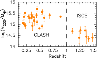
Figure 1: Cluster $M_{200}$ versus redshift for the 31 clusters for which we have halo mass estimates from the literature. Error bars on $M_{200}$ values are taken from the literature. The dashed line separates the CLASH and ISCS subsets.

$M_{200}$ estimates for six of our ISCS clusters are taken from Jee et al. (2011), who used a weak-lensing analysis. Brodwin et al. (2011) measured the cluster mass of ISCS J1432.4$+$3250 using Chandra X-ray observations. For the remaining ISCS clusters in our sample, which do not have published M₂₀₀ estimates, their halo masses can be taken to be the average sample halo mass of $M_{200}\sim 10^{14}\,M_{\odot}$, inferred from an analysis of the correlation function of the entire set of ISCS clusters (Brodwin et al., 2007).

Figure 1 shows $M_{200}$ as a function of redshift for each cluster in our sample, excluding those for which we do not have published mass estimates. Given the large differences between the $M_{200}$ of CLASH and ISCS clusters, we must now determine whether the latter clusters could be the likely progenitors of any of the 24 CLASH clusters for which we have $M_{200}$ estimates. Should that be the case, it would follow that the galaxies that reside in these high-redshift clusters can be considered likely progenitors of the CLASH galaxies at $z<1$.

We model the mass growth of our clusters across the entire redshift range of our sample with the code COncentration-Mass relation and Mass Accretion History (COMMAH; Correa et al., 2015a, b, c), which uses an analytic model to generate halo mass accretion rates for a variety of redshifts ($\Delta z=0.25$) and cluster masses ($\Delta\log\left(M_{200}\right)=0.2$). In addition to the code itself, Correa et al. (2015a, b, c) provide tabulated accretion rates for a number of different cosmologies.

Table 2: $M_{200}$ Evolutionary Track Parameters

Cluster	$t_{0}$	$M_{200}$	$d\left(M_{200}\right)/dt_{\mathrm{L}}$
	(Gyr)	($10^{14}\,M_{\odot}$)	$M_{\odot}\,\mathrm{yr}^{-1}$
MACS 1311.0$+$0310	$5.0$	$6.5$	$10^{5.0}$
MACS 0744.9$+$3927	$6.3$	$25.6$	$10^{5.9}$
ISCS J1429.3$+$3437	$8.7$	$5.4$	$10^{5.5}$
ISCS J1432.4$+$3250	$9.4$	$2.5$	$10^{5.1}$

We compare our sample to their tabulated grids, selecting accretion rates for four clusters where both the total masses and redshifts agree well (differences of no more than 0.07 and 0.06 in $\log\left(M_{200}/M_{\odot}\right)$ and redshift, respectively). We list these clusters in Table 2, along with the lookback time at their redshift, $M_{200}$ at their redshift, and mass accretion rate. With the given accretion rate, a cluster’s mass can be projected as a function of time through

$$M_{200}\left(t_{\mathrm{L}}\right)=-\left(t_{\mathrm{L}}-t_{0}\right)\frac{d\left(M_{200}\right)}{dt_{\mathrm{L}}}+M_{200}\left(t_{0}\right),$$ (1)

where $t_{\mathrm{L}}$ is the lookback time (the negative slope comes from this dependence), $d\left(M_{200}\right)/dt_{\mathrm{L}}$ is the mass accretion rate, $M_{200}\left(t_{0}\right)$ is a cluster’s mass at its observed redshift, and $t_{0}$ is the lookback time at that redshift.

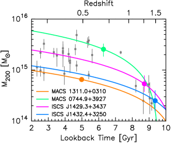
Figure 2: Cluster $M_{200}$ versus lookback time for clusters in our sample that have published mass estimates. The circles highlight the clusters listed in Table 2, with the corresponding colored curves showing their projected mass evolution, described by Equation (1) with parameters from Table 2.

Figure 2 shows the evolutionary tracks based on Equation (1) for our selected clusters. Also shown are the measured cluster $M_{200}$ values as a function of lookback time, with the bulk of our sample plotted with gray squares. The four chosen clusters are shown with circles that match the color of their respective time-dependent mass track.

Figure 2 can be understood in two ways. It may either tell us about the unevolved mass of a cluster at earlier lookback times considering its current (low-redshift) mass, or it may inform us about the evolution of a high-redshift cluster’s $M_{200}$ up to recent times. Considering first the two selected ISCS clusters, their tracks are found to intersect with a number of CLASH clusters (at least within their uncertainties). For instance, given its expected mass accretion, the cluster ISCS J1432.4$+$3250 at $z=1.49$ (blue curve) could conceivably evolve into an A383-sized cluster ($M_{200}\sim 10^{15}\,M_{\odot}$). Tracing the potential evolution of ISCS J1429.3$+$3437 at $z=1.26$ (magenta curve), it could also well evolve into a massive cluster, up to $\sim$$2\times 10^{15}\,M_{\odot}$.

While neither of the ISCS tracks overlap with the most massive CLASH clusters, we now consider the backwards evolution (with increasing lookback time) of the $z=0.69$ cluster MACS0744 (green curve). Given its projected growth rate, it could be considered as a mid-evolutionary phase between the low-mass clusters we observe at $t_{\mathrm{L}}\sim 9$ Gyr and the $\sim$$\left(3-5\right)\times 10^{15}\,M_{\odot}$ CLASH clusters. Based on its predicted evolution, MACS1311 ($z=0.49$; orange curve) provides a link between the low-mass (for our samples) cluster regime at all considered lookback times/redshifts. The good agreement seen in Figure 2 between the measured and inferred cluster $M_{200}$ values suggests that ISCS members are, in an aggregate sense, the likely progenitors of CLASH cluster galaxies.

3 Galaxy Data and Sample Selection

We now describe the selection of cluster members (Section 3.1), morphological classification of CLASH and ISCS galaxies (Section 3.2), removal of BCGs (Section 3.3) and galaxies that host AGNs (Section 3.4), and the measurement of SFRs and stellar masses (Section 3.5).

3.1 Selecting Cluster Members

3.1.1 ISCS

In Paper I, the selection of ISCS cluster members used two different methods. First, galaxies were considered members if they had high-quality spectroscopic redshifts consistent with ISCS cluster redshifts (Eisenhardt et al., 2008; Brodwin et al., 2013; Zeimann et al., 2013). Second, if no high-quality $z_{\mathrm{spec}}$ was available, ISCS galaxies were deemed members if they belong to the cluster red-sequence as determined by Snyder et al. (2012) with HST photometry. Of the 270 ISCS cluster members, 69 are selected with spectroscopic redshifts, and 201 based on galaxy colors. Using the published table of spectroscopic redshifts from Zeimann et al. (2013), we identify 43 confirmed non-members that were included in the red-sequence analysis of Snyder et al. (2012). Of these galaxies, 11 would have been considered cluster members based on their color, for a field contamination rate of $\sim$26%.

3.1.2 CLASH

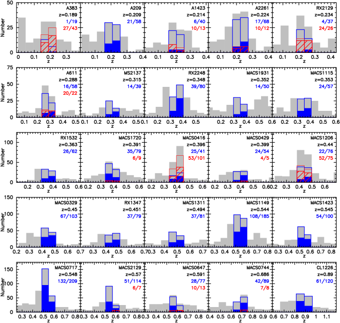
Figure 3: Histograms of $z_{\mathrm{spec}}$ (red open) and $z_{\mathrm{phot}}$ (blue open) CLASH members, superimposed over the best available redshift of the entire CLASH sample (gray). Filled blue (hashed red) histograms show the final sample of CLASH $z_{\mathrm{phot}}$ ($z_{\mathrm{spec}}$) members. Each panel shows the shortened cluster name, $z_{\mathrm{cluster}}$, and final number of $z_{\mathrm{phot}}$ (blue) and $z_{\mathrm{spec}}$ members (red) over the total number of each. Members not meeting the cuts described throughout the text are not plotted.

As part of our CLASH membership selection, we prune likely stars from our final sample by removing objects with the SExtractor (Bertin & Arnouts, 1996) stellarity parameter $\mathrm{CLASS\_STAR}>0.85$.

Spectroscopic Redshifts

While all CLASH clusters likely have spectroscopic redshifts measured for a small number of members, the literature provides extensive catalogs of publicly available spectroscopic redshift measurements for galaxies in a subset of the 25 CLASH systems. The selections, described below, result in 334 spectroscopic members.

The ongoing CLASH-VLT program (Rosati et al., 2014) will provide an unprecedented number of spectroscopic redshifts in 24 of the 25 CLASH fields once completed. We take advantage of spectroscopic redshifts for the two CLASH-VLT clusters publicly released: MACS0416 (Balestra et al., 2016) and MACS1206 (Biviano et al., 2013). For MACS1206, we use the list of cluster members provided by Girardi et al. (2015), where the membership was determined using the technique for selecting cluster members from Fadda et al. (1996). In this method, the peak in the spectroscopic redshift distribution is found and galaxies are iteratively rejected if their redshifts lie too far from the main distribution. Balestra et al. (2016), who used the same method for determining cluster membership, did not include a membership flag in the MACS0416 catalog. However, as all of our potential MACS0416 members are contained within $R_{\text{proj}}\lesssim 0.7\,\mathrm{Mpc}$, we use $cz\leq\pm 2100\,\mathrm{km}\,\mathrm{s}^{-1}$ as our membership criterion, based on the extent of cluster members at that radius (see Figure 6 of Balestra et al., 2016).

We use spectroscopic redshifts for A383 from Geller et al. (2014), A611 from Lemze et al. (2013), and for A1423, A2261, and RXJ2129 from Rines et al. (2013). For each of these five clusters, membership was determined via caustic techniques (Diaferio & Geller, 1997; Diaferio, 1999). For A383, A1423, A2261, and RXJ2129, the authors included a membership flag in their published redshift tables; we use this flag to select spectroscopic members for these four clusters. For A611, spectroscopic members are based on an unpublished membership list (D. Lemze, private comm.).

We further supplement our catalog with spectroscopic redshifts for candidate members in MACS1720, MACS0429, MACS2129, MACS0647, and MACS0744 from the catalog published by Stern et al. (2010). After removing star-like objects, we include as cluster members galaxies with $-0.02<z_{\mathrm{spec}}-z_{\mathrm{cluster}}<0.03$, based on the peak in the distribution of redshift residuals.

Photometric Redshifts

To select the remainder our our $z<1$ cluster members we use photometric redshift estimates derived by Postman et al. (2012) using Bayesian Photometric Redshift (Benítez, 2000; Benítez et al., 2004; Coe et al., 2006), a Bayesian $\chi^{2}$ minimization template fitting software package. Each galaxy’s photometric redshift was given an odds parameter, $P\left(z\right)$, defined as the integral of the probability distribution in a region of $\sim$$2\left(1+z_{\mathrm{phot}}\right)$ around $z_{\mathrm{phot}}$. A value near unity indicates that the distribution has a narrow single peak (Benítez et al., 2004) and our final sample only contains galaxies with $P\left(z\right)>0.9$, considered to be the most reliable by Postman et al. (2012). For a galaxy to be a cluster member, we require that its $z_{\mathrm{phot}}$ be contained within $z_{\mathrm{cluster}}\pm 0.04\times\left(1+z_{\mathrm{cluster}}\right)$.

In order to estimate the potential field contamination of selecting cluster members by their photometric redshifts we identify the 172 galaxies in our initial CLASH sample that are confirmed non-members according to their spectroscopic redshifts. Of these, 45 have $z_{\mathrm{phot}}$ consistent with being members, for a field contamination rate of $\sim$26%.

Cluster Members

Figure 3 shows the distribution of photometric and spectroscopic redshifts for the CLASH members. The 334 $z_{\mathrm{spec}}$ members are plotted as the red open histograms, while the 1975 $z_{\mathrm{phot}}$ members are depicted by the blue open histograms. Cluster names and redshifts are listed. Due to cuts on BCGs (Section 3.3), presence of an AGN (Section 3.4), morphology (Section 3.2), filter requirements for SED fitting (Section 3.5.2), and stellar mass (Section 3.5.3) the final CLASH sample contains 1134 galaxies. The red hatched (blue filled) histograms show the 229 (905) final spectroscopic (photometric) members.

3.2 Galaxy Morphology

Figure 4: Pseudocolor cutouts (left column) of example visually classified ETGs (top three rows) and LTGs (bottom three rows), with morphology and cluster redshift listed for each galaxy. A scale of $1\arcsec$ is shown by the white line in each pseudocolor image. The right three columns show the blue, green, and red filters that comprise each pseudocolor image and that were used for visual classification. Each image is 30x30 kpc.

In Paper I, galaxies were visually classified using observed-frame HST optical images, taken with either the Advanced Camera for Surveys (ACS; Ford et al., 1998) or the Wide Field Planetary Camera 2 (Holtzman et al., 1995), and near-infrared images, acquired with the Wide Field Camera 3 (WFC3; Kimble et al., 2008). ETGs were required to have a smooth elliptical/S0 shape, while galaxies that showed clear spiral structure, or irregular or disturbed morphologies, were collectively classified as LTGs. For consistency with Paper I, we similarly visually classify the morphology of CLASH members. Given the broad spectral coverage afforded by CLASH, we simultaneously inspect at least one HST image in each of the ultraviolet, optical and near-infrared. We could not cleanly assess the morphology for a small subset of galaxies. The latter are thus left out of any forthcoming analysis.

Figure 4 shows examples of visually classified ETGs and LTGs, spanning the majority of the redshift range of our sample. While the visual classification was performed by simultaneously inspecting single-band HST images (shown in the three rightmost columns, with filter listed), we also provide pseudocolor cutouts in the left column.

3.3 Excluding Brightest Cluster Galaxies

BCGs are typically the dominant, central galaxy in the cluster environment and are thought to have undergone an evolution different to that of the rest of the cluster population (Groenewald & Loubser, 2014; Donahue et al., 2015, and references therein). Because of their potentially different histories and sometimes elevated SF activity (e.g., McNamara et al., 2006; McDonald et al., 2013, 2016), we remove them from our analysis.

The positions of all galaxies in our CLASH sample are compared with the CLASH BCGs studied by Donahue et al. (2015, their Table 4). We do not find a match for eight of their BCGs as our own selection criteria already singled out these galaxies. We inspect each pair of the remaining matched sources in rest-frame ultraviolet and optical HST images to ensure that the object is indeed the cluster BCG. This results in the elimination of 17 additional BCGs across all 25 CLASH clusters.

In a manner similar to the BCG identification method of Lin et al. (2013) we identify potential ISCS BCGs by first selecting the $\sim$5 galaxies in each of the 11 ISCS cluster fields that have the highest $4.5\,\mu$m flux. However, none of these 56 galaxies match our final list of ISCS members. We are confident that our cluster sample is free of BCGs.

3.4 AGN Removal

Since AGNs contribute to galaxies’ infrared flux and can potentially contaminate our SFRs and stellar masses, we remove their host galaxies from our sample. Following Paper I, we identify AGNs using the IRAC color-color selection from Stern et al. (2005). Unlike that treatment, however, we do not remove galaxies with fewer than four good IRAC fluxes. Additionally, all ISCS galaxies with hard X-ray luminosities exceeding $10^{43}\,\mathrm{erg}\,\mathrm{s}^{-1}$ are removed. This results in the removal of 17 cluster members.

3.5 Estimating Physical Properties of Cluster Galaxies

3.5.1 ISCS

Paper I used IRAC observations as positional priors to match the MIPS fluxes to HST catalog sources. The Chary & Elbaz (2001) templates were used to convert the measured 24 $\mu$m fluxes to total IR luminosities, then SFRs were calculated using relation (4) from Murphy et al. (2011). Using HST images, ISCS members were visually inspected to determine isolation. Galaxies with nearby neighbors were removed from the final sample, as their mid-infrared SFRs could not be reliably measured due to the large MIPS point spread function. For consistency with our CLASH sample, here we calculate ISCS SFRs through SED fitting. We describe this procedure in Section 3.5.2, and in Appendix A we present a comparison of these SFRs and the 24 $\mu$m SFRs from Paper I.

Stellar masses were estimated in Paper I by fitting galaxies’ SEDs to population synthesis models using iSEDfit (Moustakas et al., 2013), the Bruzual & Charlot (2003) stellar population models, and the Chabrier (2003) IMF. As with the ISCS SFRs, we re-derive stellar masses as described in the following section, and compare them to the values calculated with iSEDfit in Appendix A.

Photometry for our ISCS galaxies includes three NDWFS optical wavebands ($B_{w}$, $R$, and $I$), three near-infrared bands from the FLAMINGOS Extragalactic Survey ($J,\;H$, and $K_{s}$; Elston et al., 2006), one near-infrared HST band (F160W), and five Spitzer bands (3.6, 4.5, 5.8, and 8.0 $\mu$m on IRAC, and 24 $\mu$m on MIPS). Despite the small number of bands relative to CLASH, the ultraviolet portion of the spectrum is well-covered at $z\sim 1$ by the $B_{w}$ and $I$ filters, with $R$ band straddling the ultraviolet and optical regimes. F160W and all four bands of IRAC provide good coverage of the infrared. In the range of $z\sim 1.5$, F814W and $R$ now also sample the ultraviolet, while F160W falls into the redshifted optical regime. While we do have 24 $\mu$m MIPS observations, we exclude them from our final SED fits in order to be more inclusive of non-isolated galaxies. We discuss the validity of this choice in Appendix A.

3.5.2 Spectral Energy Distribution Fitting

To estimate the SFRs and stellar masses for all galaxies in our sample we use the Code Investigating GALaxy Emission (CIGALE; Burgarella et al., 2005; Noll et al., 2009; Roehlly et al., 2012, 2014). Combining various models, each encompassing a number of free parameters, CIGALE builds theoretical SEDs, using the energy balance approach, in which (conceptually) a portion of a galaxy’s flux is absorbed in the ultraviolet with a corresponding re-radiation in the infrared, with the latter balancing the total energy of the system. CIGALE then compares the theoretical SEDs to multi-wavelength observations, generating a probability distribution function for each parameter of interest.

The input data for each galaxy in our sample are its unique identifier, redshift, and the flux and associated errors in each observed filter. With CIGALE’s energy balance approach in mind, we only include galaxies that have good fluxes in at least one rest-frame filter in each the ultraviolet and near-infrared. To reduce computational time during the SED modeling, we set the redshift of each member galaxy to its parent cluster’s redshift. For all CIGALE runs we adopt a Bruzual & Charlot (2003) stellar population model, with a Chabrier (2003) IMF, and solar metallicity. Table 3 lists the CIGALE parameters that define the template SEDs for all galaxies.

Table 3: CIGALE Input Parameters

Parameter	Values
Double declining exponential star formation history
$\tau_{\mathrm{main}}$ (Gyr)	$0.5-5$
$\tau_{\mathrm{burst}}$ (Gyr)	10
$t_{\mathrm{main}}$ (Gyr)	$1-11$
$t_{\mathrm{burst}}$ (Myr)	$50-750$
$f_{\mathrm{burst}}$	$0-0.2$
Dust attenuation: Calzetti et al. (2000) and Leitherer et al. (2002)
$E\left(B-V\right)_{\star,\mathrm{young}}$	$0-1$
Dust template: Dale et al. (2014)
$f_{\mathrm{AGN}}$	0
$\alpha_{\mathrm{dust}}$	$1-3$

Star formation histories (SFHs) commonly found in the literature include a single stellar population with an exponentially declining SFR, a single stellar population with an SFR that declines exponentially after some delay time, or a two-component exponentially declining model consisting of a recently formed young stellar population on top of an underlying old stellar population. As galaxies are expected to undergo multiple SF episodes, this latter type of SFH is better suited than a single-population SFH to model complex stellar systems (Buat et al., 2014). However, Ciesla et al. (2016) have recently shown promising results using a truncated delayed SFH to model the rapid quenching expected of galaxies undergoing ram-pressure stripping in the cluster environment. While a comparison of the physical properties of CLASH galaxies derived by different SFHs will be reviewed elsewhere, we adopt a double declining exponential SFH in this work.

The SFR in a declining exponential SFH is characterized by

$$SFR\left(t\right)\propto e^{-t/\tau},$$ (2)

where $t$ is time (i.e., the age of the stellar population) and $\tau$ is the $e$-folding time. As our adopted SFH comprises an old (main) and younger (burst) stellar population, each has an age ($t_{\mathrm{main}}$ and $t_{\mathrm{burst}}$, respectively) and an $e$-folding time ($\tau_{\mathrm{main}}$ and $\tau_{\mathrm{burst}}$, respectively). Prior to the burst occurring ($t<t_{\mathrm{main}}-t_{\mathrm{burst}}$), the galaxy forms stars according to Equation (2). Subsequently, the SFR of the galaxy is modeled as a linear combination of two such functions, with the exponential component for the young stellar population modulated by a burst fraction ($f_{\mathrm{young}}$), which defines the mass fraction contributed by young stars. To generate a wide array of possible galaxy histories, we supply CIGALE with a range of values for $t_{\mathrm{burst}}$, $t_{\mathrm{main}}$, and $\tau_{\mathrm{main}}$. We approximate a constant burst of SF for the young population by fixing its $e$-folding time at 10 Gyr. The remaining parameters listed in Table 3 are the dust attenuation of the young population ($E(B-V)_{\star,\mathrm{young}}$), the fraction of infrared emission due to an AGN ($f_{\mathrm{AGN}}$), and the infrared power law slope ($\alpha_{\mathrm{dust}}$). As we remove AGNs from our entire cluster sample (Section 3.4), we fix $f_{\mathrm{AGN}}=0$ for all models. While we have removed galaxies with a dominating AGN component, there may be some subdominant AGN contribution to the measured SFRs of the remainder of our sample. However, disentangling such low-level contribution is beyond the scope of this work.

3.5.3 Star Formation Rates and Stellar Masses

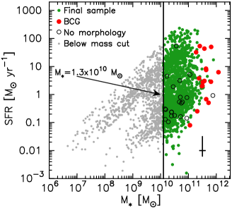
Figure 5: CIGALE-derived SFR versus stellar mass for cluster members, with our final sample plotted with green points. Also shown are galaxies cut from the sample (see legend), as well as the stellar mass cut (vertical line). Galaxies identified as likely AGN hosts (Section 3.4) are not plotted. The error bar in the lower right corner shows the typical uncertainty in the SFRs and stellar masses derived with CIGALE.

Figure 5 shows the CIGALE-derived SFRs and stellar masses for our cluster sample. In addition to the sample cuts described up to this point, we impose a further cut on our sample by requiring all galaxies to meet the 80% mass completeness limit of Paper I, $\log\left(M_{\star}/M_{\odot}\right)>10.1$. Galaxies that fall above our stellar mass cut (to the right of the vertical line) for which we could not reliably determine a morphology (Section 3.2) are plotted with open black circles. We do not identify all galaxies without a morphology as many of the galaxies that fall below our mass cut were not inspected for morphology. BCGs identified in Section 3.3 are shown by the red points and our final sample ($N=1386$) is shown by the green circles. Table 2 gives the breakdown by cluster of the number of cluster members ($N_{\mathrm{tot}}$), ETGs ($N_{\mathrm{ETG}}$) and LTGs ($N_{\mathrm{LTG}}$) in our final sample.

3.5.4 Separating Star-forming and Quiescent Galaxies

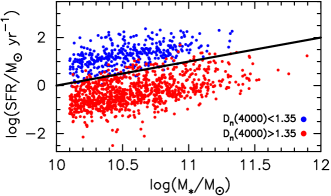
Figure 6: SFR-$M_{\star}$ plane for SFGs (blue) and quiescent galaxies (red) defined by a $D_{n}\left(4000\right)=1.35$ cut. The black line shows a constant specific SFR of $SFR/M_{\star}=0.1\,\mathrm{Gyr}^{-1}$.

In addition to classifying cluster galaxies based on their morphologies, we separate members based on whether they are still actively forming new stars (star-forming galaxies; SFGs) or are quiescent (i.e., have little to no ongoing SF). These two galaxy types are commonly separated on the basis of the strength of the 4000 Å break, which is an indicator of their stellar population age (Bruzual, 1983; Balogh et al., 1999; Kauffmann et al., 2003). The amplitude of the break, $D_{n}\left(4000\right)$, is used to separate galaxies into young (star-forming) and old (quiescent) galaxies (e.g., Vergani et al., 2008; Woods et al., 2010). Our SED fits enable a recovery of $D_{n}\left(4000\right)$, which CIGALE calculates as the ratio of the flux in the red continuum (4000–4100 Å) to that in the blue continuum (3850–3950 Å), based on the definition of Balogh et al. (1999).

We adopt a cutoff of $D_{n}\left(4000\right)<1.35$ (Johnston et al., 2015) to select SFGs, which results in 392 star-forming and 994 quiescent cluster members. Table 2 lists the final number of SFGs ($N_{\mathrm{SFG}}$) and quiescent galaxies ($N_{\mathrm{Q}}$) in each cluster, and Figure 6 shows the SFR versus stellar mass of each subset. Another common metric for selecting SFGs (e.g., Lin et al., 2014) is the specific SFR ($sSFR\equiv SFR/M_{\star}$), which measures a galaxy’s efficiency at forming new stars. For comparison, we find that a constant sSFR of $0.1\,\mathrm{Gyr}^{-1}$ (black line) qualitatively agrees with our $D_{n}\left(4000\right)$ cut. We reinforce that our selection of ETGs and LTGs in Section 3.2 was based on their morphologies and should not to be confused with spectroscopically early- and late-type galaxies, terms that are sometimes used to refer to quiescent and star-forming galaxies, respectively (e.g., Vergani et al., 2008).

4 Results and Discussion

Throughout this section, we incorporate into our error bars the uncertainty due to the potential field contamination of the cluster members selected with photometric redshifts or through red-sequence color selection (see Section 3.1). Error bars on fractional values are calculated as the quadrature sum of uncertainties based on binomial confidence intervals (Gehrels, 1986) and those due to potential field contamination. The latter are the differences between the calculated fraction and the bounds of the fraction assuming 26% of the $z_{\mathrm{phot}}$/color-selected subset contained interlopers. The error bars on sSFR values are calculated as the quadrature sum of simple Poisson errors and 5000 iterations of bootstrap resampling. To calculate the former, the number of galaxies used in each bin is the sum of the number of $z_{\mathrm{spec}}$ members and 74% of the number of $z_{\mathrm{phot}}$/color-selected members (to simulate a 26% interloper rate). For each iteration of bootstrap resampling, pairs of SFR and stellar mass are chosen from the set of spectroscopically-selected members and a random sampling of 74% of the non-$z_{\mathrm{spec}}$ members.

4.1 The Relation Between SFR and Stellar Mass in Cluster SFGs

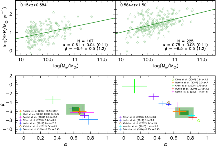
Figure 7: Upper panels: SFR versus $M_{\star}$ for cluster SFGs (light green stars). SFGs are fit (dark green lines) by Equation (3), with the number of galaxies, fit coefficients, and 1$\sigma$ and total (when accounting for potential field contamination; see text) uncertainties listed. Lower panels: Comparison of SFR-$M_{\star}$ parameters for our best fit, with 1$\sigma$ (dark green rectangles) and total (light green rectangles) uncertainties shown. A selection of literature best-fit parameters, calibrated by Speagle et al. (2014), are provided: Elbaz et al. (2007); Noeske et al. (2007); Chen et al. (2009); Dunne et al. (2009); Santini et al. (2009); Oliver et al. (2010); Karim et al. (2011); Whitaker et al. (2012); Kashino et al. (2013); and Sobral et al. (2014). Colored error bars show the parameter uncertainties (if available) from the literature; best-fit parameters with no uncertainties are shown by open circles.

SFR (or sSFR) as a function of stellar mass, hereafter referred to as the SFR-$M_{\star}$ relation, has been studied extensively over the last decade, resulting in a tight correlation between these two physical quantities, often referred to as the “main sequence” of SF (Noeske et al., 2007; Elbaz et al., 2011). This is often characterized by a power law of the form

$$\log\left(SFR/M_{\odot}\,\mathrm{yr}^{-1}\right)=\alpha\log\left(M_{\star}/M_{\odot}\right)+\beta,$$ (3)

where $\alpha$ and $\beta$ are the slope and normalization, respectively. The SFR-$M_{\star}$ relation as a function of redshift has been investigated in numerous studies (e.g., Vulcani et al., 2010; Ilbert et al., 2015; Schreiber et al., 2015; Tasca et al., 2015). Speagle et al. (2014) compiled and standardized a sample of 25 studies from the literature over the range of $0<z<6$ and found that despite a variety of SFR and stellar mass indicators, there is a good consensus on the SFR-$M_{\star}$ relations, with a 1$\sigma$ scatter of $\sim$0.1 dex among publications. Although Speagle et al. (2014) calibrated the literature fits to a Kroupa (2001) IMF, they note that differences between this and the Chabrier (2003) IMF we employ have a negligible impact on the coefficients of the SFR-$M_{\star}$ relation.

While studies of the SFR-$M_{\star}$ relation have largely focused on field SFGs, higher-density environments have received more recent attention (e.g., Greene et al., 2012; Jaffé et al., 2014; Lin et al., 2014; Erfanianfar et al., 2016). Along those lines, we plot SFR versus stellar mass in the upper panels of Figure 7, for the star-forming cluster galaxies (green stars) selected in Section 3.5.4. Our cluster SFGs are separated into two broad redshift bins, $0.15<z<0.584$ and $0.584<z<1.5$, each spanning $\sim$3.75 Gyr in lookback time. The galaxies are fitted (dark green lines) with Equation (3) and the results are reported in each panel. Despite the considerable scatter in our SFR-$M_{\star}$ fits, the standard deviation of 0.38 at $0.15<z<0.584$ is similar to the observed 1$\sigma$ scatter in the literature, which ranges from 0.15 to 0.61, as compiled by Speagle et al. (2014) for studies where the redshift ranges overlap with ours. Similarly, over $0.584<z<1.5$, our 1$\sigma$ scatter of 0.36 is consistent with the corresponding range (0.09 to 0.47) of measured standard deviations reported by Speagle et al. (2014). Shown in the upper panels are 1$\sigma$ uncertainties per parameter derived using the formalism from Press et al. (1992), assuming the uncertainty of each ordinate value is the mean SFR uncertainty. The total uncertainties, shown in parenthesis, account for possible field contamination in the non-spectroscopically selected cluster SFGs. We devise a Monte Carlo realization to calculate the uncertainty due to potential interlopers, whereby 74% of the $z_{\mathrm{phot}}$/color-selected subset (to simulate a 26% interloper rate; see Section 3.1) are randomly selected. These galaxies are combined with the $z_{\mathrm{spec}}$ members and a new fit is re-derived. This is performed 5000 times in each redshift bin, and the standard error is calculated for the 5000 sets of parameters. The standard error is added in quadrature with the 1$\sigma$ uncertainty to derive a total parameter uncertainty.

In the lower panels of Figure 7, we show our best-fit $\alpha$ and $\beta$, with corresponding uncertainties, along with a sample of best-fit SFR-$M_{\star}$ parameters and uncertainties (if available) from the literature, as calibrated and provided by Speagle et al. (2014). Given the consistency of our fits with those from the literature, this suggests that (even when accounting for any potential contamination from interlopers) the SFR-$M_{\star}$ relation of star-forming cluster galaxies is robust and effectively the same as that of field SFGs, echoing similar conclusions by, e.g., Greene et al. (2012), Koyama et al. (2013), and Lin et al. (2014).

4.2 The Impact of Stellar Mass on Star-forming and Quiescent Cluster Galaxies

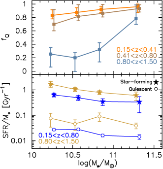
Figure 8: Upper panel: Fraction of quiescent cluster galaxies as a function of stellar mass. Lower panel: Specific SFR versus stellar mass for cluster SFGs (stars) and quiescent galaxies (open circles). Points have been slightly offset for clarity.

The upper panel of Figure 8 shows the fraction of quiescent cluster galaxies, $f_{\mathrm{Q}}$, as a function of stellar mass. Given our stellar mass binning, three cluster galaxies with $\log\left(M_{\star}/M_{\odot}\right)>11.6$ are excluded. Their removal plays no role in our final results. In each stellar mass bin, galaxies are separated into three redshift slices, each spanning $\sim$2.5 Gyr of lookback time (see legend for color coding).

The fraction of quiescent galaxies and stellar mass are correlated, regardless of redshift. However, the increase in $f_{\mathrm{Q}}$ with stellar mass is relatively mild at $z\sim 0.3$ and $z\sim 0.6$, and given the uncertainties, formally consistent with no trend. Over $0.2<z<0.5$ and $0.5<z<0.8$, which are similar to our two lower redshift bins, Lin et al. (2014) found $f_{\mathrm{Q}}$ values that are uniformly lower at $\log\left(M_{\star}/M_{\odot}\right)\lesssim 11.3$, even when accounting for the difference between their adopted Salpeter (1955) IMF and our Chabrier (2003) IMF. While Lin et al. (2014) did not provide the halo mass range of their sample, they differentiated between groups and clusters based on richness. Their cluster selection corresponds to halo masses $\gtrsim$$10^{14}\,M_{\odot}$, which is nearly an order of magnitude lower than the minimum $M_{200}$ of our cluster sample over the same redshift range ($\sim$$8\times 10^{14}\,M_{\odot}$). As quiescent galaxies tend to populate more massive halos at a given stellar mass (Lin et al., 2016), the large difference in the underlying properties of the two cluster samples may explain the substantial differences in $f_{\mathrm{Q}}$.

The high fraction of quiescent galaxies at $z\lesssim 0.8$ implies that most of the passive cluster population was being built up at earlier times. Since the most massive cluster galaxies ($\log\left(M_{\star}/M_{\odot}\right)\sim 11.3$) are almost uniformly passive as far back as $z\sim 1.2$, this build up can be attributed to the quenching of lower-mass galaxies at (or above) this redshift.

Quiescent fraction and stellar mass are more strongly correlated at $z\sim 1.2$ than at $z\sim 0.3$ or $z\sim 0.6$, with $\Delta f_{\mathrm{Q}}=0.53$ over the same stellar mass range as in the two lower redshift bins. Qualitatively, this matches the results of Balogh et al. (2016) for galaxies in $\log\left(M_{200}/M_{\odot}\right)\sim 14.5$ clusters at $z\sim 1$, although they found that $f_{\mathrm{Q}}$ rises sharply at $\log\left(M_{\star}/M_{\odot}\right)\sim 10.5$, followed by a gradual increase up to $\log\left(M_{\star}/M_{\odot}\right)\sim 11.3$. The correlation between $f_{\mathrm{Q}}$ and $M_{\star}$ above $z=0.8$ suggests that quenching is ongoing at this epoch and the build up of stellar mass plays a role in turning off the SF activity of SFGs. Lee et al. (2015) found a strong correlation between quiescent fraction and stellar mass for candidate cluster galaxies over $1<z<1.5$, which they also attribute to mass quenching.

Some portion of the increase in quiescent fraction over time at fixed mass, however, is likely due to the accretion of previously-quenched galaxies from lower-density environments into clusters (pre-processing; e.g., Haines et al., 2015). Regardless of the method by which cluster galaxies are quenched, or even whether they fall into the cluster environment pre-quenched, it is the increasing quiescent fraction that drives the strong evolution in the SF activity of the overall cluster population with time (Section 4.3).

In the lower panel of Figure 8 we consider the SF efficiency of our cluster galaxies as a function of stellar mass. Due to the paucity of low-redshift SFGs, particularly at higher stellar mass, we combine the two lower redshift bins (see legend). While $f_{\mathrm{Q}}$ shows a strong dependence on $M_{\star}$ at higher redshift, the sSFRs of both SFGs and quiescent galaxies are more mildly correlated with stellar mass. In fact, at a given redshift, there is at most a factor of $\sim$$2-3$ difference between the sSFR of the lowest- and highest-mass cluster galaxies within each subset. We find a similar trend in the tabulated results of Lin et al. (2014), over the same stellar mass range that we study, and the cluster galaxy sSFRs measured by Muzzin et al. (2012) over $0.85<z<1.2$ align extremely well with ours at $0.8<z<1.5$. While the build up of stellar mass appears linked to transitioning galaxies between the star-forming and quiescent populations, stellar mass has less of an impact on the SF efficiency of galaxies within each distinct subset.

4.3 The Evolution of Cluster Galaxies: The Mixing of Two Distinct Populations

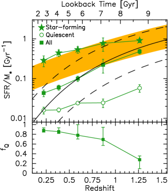
Figure 9: Upper panel: Specific SFR versus redshift for different cluster galaxies (symbols). At all redshifts, the overall cluster population (squares) is composed of two distinct subsets: quiescent galaxies (open circles) and SFGs (stars). The sSFR of cluster SFGs is typically consistent with the SF main sequence from Elbaz et al. (2011, gold shaded region). The overall cluster sSFR is in excellent agreement with the Alberts et al. (2014) fit of sSFR versus redshift for cluster galaxies (solid black curve; dashed curves are 1$\sigma$ uncertainty). Lower panel: Fraction of quiescent cluster galaxies versus redshift. The quiescent population builds up quickly at earlier times, with fractions gradually increasing to more recent times.

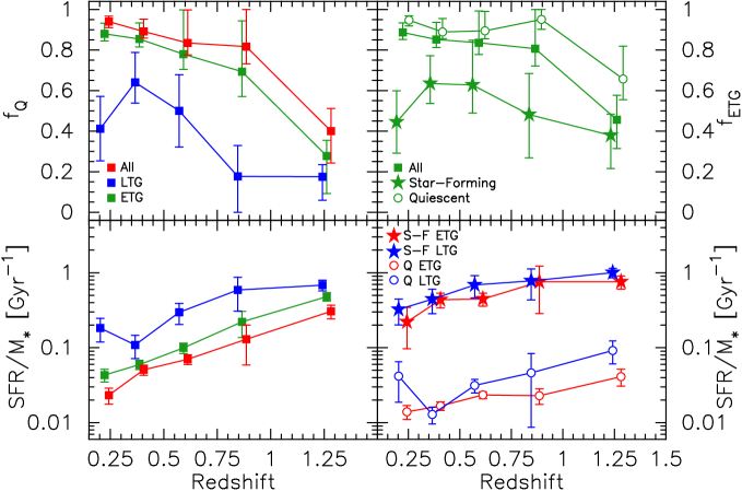
Figure 10: Upper left panel: Fraction of quiescent cluster galaxies versus redshift, separated by morphology. LTGs (blue squares) are predominantly star-forming at $z\gtrsim 0.9$; they become more evenly mixed between SFGs and quiescent galaxies below this redshift. The quiescent ETG population (red squares) builds up quickly at earlier times, with fractions gradually increasing to more recent times. The overall quiescent fraction (green squares) is well-traced by the ETGs. Upper right panel: Fraction of ETGs for different subsets of cluster galaxies. While quiescent galaxies (open circles) and the overall cluster population (squares) are predominantly early-type at all redshifts, SFGs (stars) have a more mixed morphological makeup. Lower left panel: Specific SFR versus redshift for all cluster galaxies (green squares), all ETGs (red squares), and all LTGs (blue squares). Lower right panel: Specific SFR as a function of redshift for cluster ETGs (red symbols) and LTGs (blue symbols), separated into star-forming (“S-F”; stars) and quiescent (“Q”; open circles) subsets. Independent of morphology, SFGs (and likewise quiescent cluster members) have very similar SF efficiency at all redshifts. For clarity, some points in each panel are slightly offset to the left or right of the bin center.

Given that stellar mass has a relatively mild impact on the SF efficiency of cluster galaxies when independently considering star-forming and quiescent populations, we now investigate the redshift evolution of sSFR for these two subsets, along with the overall cluster sample. The upper panel of Figure 9 shows sSFR versus redshift for all cluster galaxies (green squares), and the star-forming (green stars) and quiescent (green open circles) subsets, with galaxies separated into five redshift bins, each spanning $\sim$1.5 Gyr of lookback time.

For comparison, two sSFR fits from the literature are plotted. Elbaz et al. (2011) measured the sSFR redshift evolution of galaxies observed in the northern and southern fields of the Great Observatories Origins Deep Survey. Their best-fit sSFR evolution, which assumes $\alpha=1$ (Equation 3), describes a main sequence of

$$13\left(13.8\,\mathrm{Gyr}-t_{L}\right)^{-2.2}\leq sSFR\leq 52\left(13.8\,\mathrm{Gyr}-t_{L}\right)^{-2.2},$$ (4)

which is plotted as the gold shaded region. For a given $t_{\mathrm{L}}$, Elbaz et al. (2011) classified galaxies above this range as starbursts; galaxies that lie below $13\left(13.8\,\mathrm{Gyr}-t_{L}\right)^{-2.2}$ were considered to have “significantly lower” SF.

Alberts et al. (2014) modeled the evolution of SF activity in cluster galaxies over $0.3<z<1.5$, shown here as the solid black curve (dashed curves are the 1$\sigma$ uncertainties in their fit). Their fit only includes galaxies with cluster-centric distances of $R_{\mathrm{proj}}<0.5\,\mathrm{Mpc}$; similarly excluding all galaxies beyond this radius from our sample would not alter our qualitative results.

At all redshifts, the overall cluster population lies in good agreement with the Alberts et al. (2014) relation, with sSFR decreasing by a factor of 11 from $z\sim 1.3$ ($sSFR=0.48\pm 0.06\;\mathrm{Gyr}^{-1}$) to $z\sim 0.2$ ($sSFR=0.043\pm 0.009\;\mathrm{Gyr}^{-1}$). The SF efficiency of the SFG subset also declines over the same period, but only by a factor of 3. We find that this decline is somewhat shallower than the best-fit Elbaz et al. (2011) sSFR evolution, although our values are consistent within the uncertainties with their main sequence. That cluster SFGs have similar SF efficiency to the field population is not surprising given our results from Section 4.1, where we found that the SFR-$M_{\star}$ relation of cluster and field SFGs are consistent with each other, despite large scatters about the best fits. Quiescent cluster galaxies, which have SF efficiency $\sim$$16-31$ times lower than SFGs, experience a similar decrease in sSFR to their star-forming counterparts from $z\sim 1.3\rightarrow 0.2$, although with a slightly steeper factor of 4. As with SFGs, this evolution is more moderate than that of the overall cluster population. Thus, the strong evolution in cluster galaxy sSFR cannot simply be due to the decline in the sSFR of its constituent subsets, which experience relatively shallow decreases. Instead, as shown below, the build up of the quiescent population has a strong impact in the sSFR evolution of all cluster galaxies.

The lower panel of Figure 9 shows $f_{\mathrm{Q}}$ of all cluster galaxies as a function of redshift, using the same binning as in the top panel. At $z\sim 1.3$, the overall quiescent fraction is only $28^{+8}_{-19}\%$. Based on their relatively small contribution to the cluster population, quiescent galaxies have little impact on the overall (high) sSFR at this redshift. After a sharp rise to $f_{\mathrm{Q}}=0.69^{+0.25}_{-0.12}$ at $z\sim 0.9$, the quiescent fraction increases gradually with decreasing redshift to $z\sim 0.2$, where $88^{+5}_{-4}\%$ of cluster galaxies are quiescent. Hence, from $\sim$$7$ to 3 Gyr ago, quiescent galaxies progressively dominate the cluster population, thus lowering the SF efficiency of the overall cluster population, more so than their own moderate evolution would imply.

4.4 Star-forming and Quiescent Cluster Galaxies: Disentangling Morphology

We now explore whether the morphologies of different cluster galaxies play a role in the SF activity of the overall population. The evolution of the quiescent fraction for cluster ETGs and LTGs is plotted in the upper left panel of Figure 10, with each redshift bin spanning $\sim$1.5 Gyr of lookback time. The $f_{\mathrm{Q}}$ of cluster galaxies varies by morphology at all redshifts. While ETGs quickly build up the majority of their quiescent population at earlier times ($z\gtrsim 0.9$), LTGs are predominantly star-forming at redshifts above $z\sim 0.6$. Furthermore, over $0.15<z<1.5$, the LTG quiescent fraction is uniformly lower than that of the ETG subset, by up to a factor of $\sim$5.

As SFGs comprise a larger component of the LTG population, it would be no surprise to find that the SF activity of all cluster LTGs is higher than that of all cluster ETGs (e.g., Paper I), given the substantial difference in SF efficiency between the overall quiescent and SFG populations (see upper panel of Figure 9). Indeed, we find just such a relation for the sSFR of cluster galaxies, separated by morphology, in the lower left panel of Figure 10. Across all redshifts, cluster LTGs are $\sim$$2-8$ times more star-forming than their early-type counterparts. However, as we noted in Section 4.3, simply combining SFGs and quiescent galaxies washes out the strong differences between these two distinct types of galaxies. Instead, the morphological segregation of galaxies within the SFG subset (lower right panel of Figure 10) indicates that ETGs and LTGs have remarkably consistent sSFR values. Quiescent galaxies also show a strong agreement between ETG and LTG SF efficiency. Star-forming ETGs have SF activity $\sim$$16-33$ times higher than their quiescent counterparts; the differences between quiescent and star-forming LTGs are similar (factors of $\sim$$8-34$). At each redshift, the sSFR difference between star-forming and quiescent galaxies of the same morphology is almost uniformly an order of magnitude or more, while there is at most a minor difference between morphologies within either the SFG or quiescent subsets.

As noted in Section 4.3, the sSFR of the overall cluster population decreases by a factor of 11 from $z\sim 1.3$ to $z\sim 0.2$. This decline is larger than that of LTGs, whose SF efficiency drops by a factor of 4 (or 6 if only considering the evolution down to $z\sim 0.4$). The stronger overall evolution is due to the build up of the ETG population with time, as seen in the upper right panel of Figure 10, where we plot $f_{\mathrm{ETG}}$, the fraction of cluster galaxies classified as ETGs (squares). While $z\sim 1.3$ clusters contain a similar distribution of LTGs and ETGs, at later times, the latter become—and remain—the dominant galaxy morphology. While the SF efficiency of ETGs is no different from LTGs when accounting for ongoing SF, a higher fraction of ETGs are quiescent relative to LTGs. Thus, the confluence of these facts, combined with the increasing preponderance of ETGs, contributes to driving the observed cluster sSFR evolution.

The morphological distribution of the star-forming subset is almost uniformly distinct from that of the cluster population below $z\sim 1.3$ (upper right panel of Figure 10). While the overall cluster sample quickly becomes ETG dominated below $z\sim 1.3$, SFGs experiences a potentially more gradual rise in $f_{\mathrm{ETG}}$ with time and their ETG fraction never exceeds $\sim$$60\%$. Even though the majority of cluster ETGs are indeed passive across $0.15<z<1.5$, they still contribute approximately half of the SFG population. At higher redshifts, even as the entire cluster population acquires more late-type properties, star-forming ETGs remain prevalent (e.g., Mei et al., 2015). These results, combined with the sSFR uniformity of all cluster SFGs, suggests that the assumption that most (or all) cluster ETGs are “red and dead” oversimplifies their actual diversity.

4.5 The Uncertain Path to Quiescence

Addressing the nature and effectiveness of the quenching mechanisms at play in our CLASH and ISCS cluster galaxies is clearly challenging, however, given our results, we can draw some broad inferences. For instance, if a sizable fraction of cluster galaxies are being slowly quenched (strangulation), the SF activity of the SFG subset should (naïvely) be lower than that of field galaxies (e.g., Paccagnella et al., 2016). This is supported by Lin et al. (2014), who found that cluster SFGs over $0.2<z<0.8$ have 17% lower SF activity than field SFGs at fixed stellar mass, attributing the difference to strangulation. However, at all redshifts we study the SF activity of actively star-forming cluster galaxies is roughly equivalent to that of field SFGs (upper panel of Figure  9). While these binned sSFRs are consistent with, or even slightly higher than, the field main sequence of Elbaz et al. (2011), there are some individual SFGs ($13\pm 2\%$) that lie below this range, which may suggest that strangulation acts, at least on some level, out to at least $z=1.5$ (see also Alberts et al., 2014).

However, given the general uniformity between star-forming cluster and field sSFRs and the overall cluster galaxy quiescent fraction that increases by 0.41 from $z\sim 1.3\rightarrow 0.9$ (a time span of $\sim$1.5 Gyr), we suggest that if cluster galaxies are being quenched within the cluster environment, it must be happening relatively quickly for most of them, at least at higher redshifts. This agrees with Muzzin et al. (2012), who suggested that the lack of an environmental correlation between sSFR and $D_{n}\left(4000\right)$ in SFGs implies a rapid transition from star-forming to quiescence for $z\sim 1$ cluster galaxies. While the exact quenching method remains unsettled, there is evidence that points towards major-merger induced AGN feedback acting to quench $z\gtrsim 1$ cluster galaxies. Specifically, Paper I found that the fraction of early-type cluster galaxies increases over $z\sim 1.4\rightarrow 1.25$, and previous studies have found evidence for rapid mass assembly in $z\gtrsim 1$ clusters (Mancone et al., 2010; Fassbender et al., 2014), young galaxies continuously migrating onto the cluster red sequence (Snyder et al., 2012), and substantial (in some cases field-level) SF activity (Brodwin et al., 2013; Zeimann et al., 2013; Alberts et al., 2014; Webb et al., 2015). These results are all indicative of ongoing major-merger activity. Furthermore, the incidence of AGNs in $z\gtrsim 1$ ISCS clusters is increased relative to lower redshifts (Galametz et al., 2009; Martini et al., 2013; Alberts et al., 2016).

5 Summary

We have combined two galaxy samples of varying redshift to conduct a study of the evolution of cluster galaxy SF activity over $0.15<z<1.5$. Our final sample contains 11 high-redshift ($1<z<1.5$) ISCS clusters previously studied in Paper I (Wagner et al., 2015), and 25 low-redshift ($0.15<z<1.0$) CLASH clusters. Physical galaxy properties (i.e., SFRs and stellar masses) were measured through broadband SED fitting with CIGALE. Star-forming and quiescent cluster members were separated based on their CIGALE-derived $D_{n}\left(4000\right)$ values, and galaxies were classified into ETGs and LTGs based on their morphologies through visual inspection of high-resolution HST images.

Cluster LTGs were found to have uniformly higher SF activity than ETGs, though this is caused by an increase in the fraction of quiescent ETGs with time. At each considered redshift, star-forming ETGs have an sSFR consistent with that of late-type SFGs.

From $z\sim 1.3$ to $z\sim 0.2$, the sSFR of cluster SFGs declines by a relatively modest factor of 3. Their quiescent counterparts experience a similar (factor of 4) decrease in SF efficiency, while maintaining sSFRs at least an order of magnitude lower than SFGs. The evolution of the overall cluster sSFR, which agrees well with Alberts et al. (2014), is largely driven by the relative fraction of its constituent populations. With their sSFRs matching the field main sequence from Elbaz et al. (2011), cluster SFGs provide the dominant contribution to the overall population at higher redshifts ($z\sim 1.3$), where they comprise more than $70\%$ of the cluster population. However, as the fraction of quiescent cluster galaxies rises with decreasing redshift, up to $f_{\mathrm{Q}}=0.88^{+0.05}_{-0.04}$ at $z\sim 0.2$, their relatively low sSFRs have a much greater impact on the overall SF activity. This culminates in a factor of 11 decrease in sSFR for all massive cluster galaxies from $z\sim 1.3$ to $z\sim 0.2$.

By comparing the sSFRs of our cluster SFGs with the main sequence of Elbaz et al. (2011), we found a subset with low field-relative SF activity, which makes up $13$% of the cluster SFG population. This is indicative of strangulation acting on some level in our clusters. However, the approximately field-level SF activity of cluster SFGs and the quiescent fraction increasing by 0.41 from $z\sim 1.3\rightarrow 0.9$ would suggest that at $z\gtrsim 0.9$, the mechanism(s) quenching cluster galaxies is likely a rapid process (e.g., merger-driven AGN quenching).

While our results provide additional evidence for the rapid quenching of higher-redshift cluster galaxies, much uncertainty remains in constraining the dominant quenching mechanisms. Further study is required to better, and more quantitatively, measure the contributions of the various quenching mechanisms.

Appendix A Comparison of CIGALE-derived Star Formation Rates and Stellar Masses

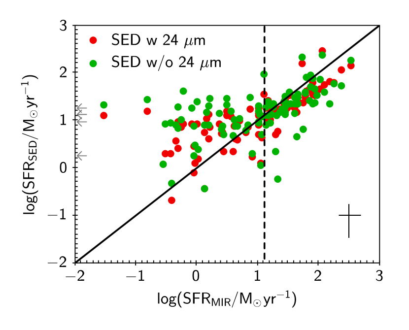
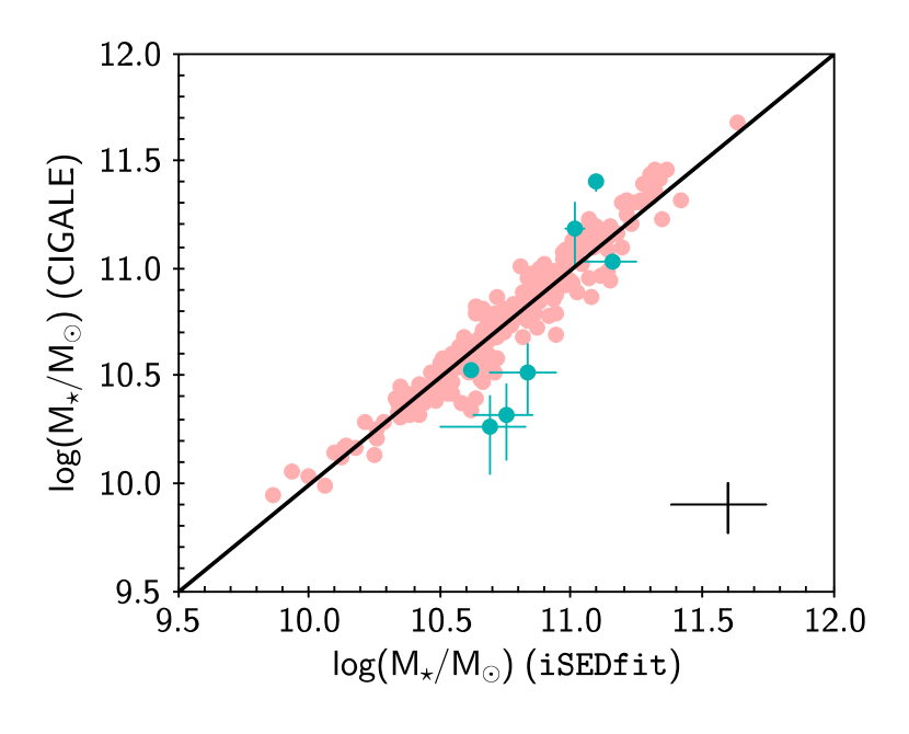
Figure 11: Upper panel: Comparison of SFRs derived through SED fitting ($SFR_{\mathrm{SED}}$) and 24 $\mu$m SFRs calculated in Paper I ($SFR_{\mathrm{MIR}}$). Galaxies plotted in red include mid-infrared fluxes in the SED fits, while those plotted in green do not. The gray arrows are the $SFR_{\mathrm{SED}}$ of galaxies undetected at 24 $\mu$m. The vertical dashed line shows the 1$\sigma$ $SFR_{\mathrm{MIR}}$ limit of $\sim$$13\,M_{\odot}\,\mathrm{yr}^{-1}$. Lower panel: Comparison of ISCS stellar masses derived with CIGALE and with iSEDfit. The galaxies highlighted in turquoise are the seven where the two measurements do not agree within the uncertainties. In both panels the solid line is a 1:1 relation, while the black error bars show the typical uncertainties in the derived properties.

The upper panel of Figure 11 shows the SFRs of isolated ISCS galaxies as measured by CIGALE ($SFR_{\mathrm{SED}}$) versus those calculated in Paper I ($SFR_{\mathrm{MIR}}$). We run CIGALE twice with the same parameters, first with 24 $\mu$m flux points, and then without. We compare $SFR_{\mathrm{SED}}$ from these runs against $SFR_{\mathrm{MIR}}$ from Paper I with red and green points, respectively. The dashed line shows the 1$\sigma$ SFR limit of $\sim$$13\,M_{\odot}\,\mathrm{yr}^{-1}$.

We find the median absolute deviation (MAD) of

$$\Delta\log\left(SFR\right)=\log\left(\frac{SFR_{\mathrm{MIR}}}{M_{\odot}\,\mathrm{yr}^{-1}}\right)-\log\left(\frac{SFR_{\mathrm{SED}}}{M_{\odot}\,\mathrm{yr}^{-1}}\right)$$ (A1)

for all galaxies plotted here, both including and excluding the 24 $\mu$m fluxes, and list them in Table 4. We similarly list the MAD for the SFR differences when only considering the galaxies above the 1$\sigma$ SFR limit.

Table 4: MAD of $\Delta\log\left(SFR\right)$ Between Paper I and CIGALE

24 $\mu$m Flux in SED	$SFR_{\mathrm{MIR}}$ Cut	MAD
	($M_{\odot}\,\mathrm{yr}^{-1}$)
Yes	$>$0	0.26
Yes	$>$13	0.11
No	$>$0	0.33
No	$>$13	0.16

When considering galaxies with low levels of 24 $\mu$m SFR, where the uncertainty in the mid-infrared is high, both CIGALE runs fail to accurately reproduce $SFR_{\mathrm{MIR}}$, as can be seen by the relatively high MADs. However, above the 1$\sigma$ level of $SFR_{\mathrm{MIR}}$, both sets of $SFR_{\mathrm{SED}}$ compare favorably, with similar scatter about the 1:1 line, and MADs that decrease by $\sim$0.15. Given that the $SFR_{\mathrm{SED}}$ values calculated with and without mid-infrared fluxes are similar, we opt to use the latter in our analysis. This provides the additional benefit of allowing us to include non-isolated ISCS galaxies in our analysis, as our SED fits are not contingent on observations with poor resolution inherent to the mid-infrared. By including non-isolated ISCS galaxies, the $z>1$ portion of our sample has 255 galaxies after all selection cuts are applied, $\sim$2.5 times as many as it would have had if only allowing isolated galaxies.

The lower panel of Figure 11 shows stellar masses derived by CIGALE versus those derived by iSEDfit. The salmon colored points are the galaxies where the two values agree within their uncertainties, while the turquoise points show the seven galaxies where the stellar masses do not agree. Overall, CIGALE and iSEDfit agree well with each other. We find a MAD of $\Delta\log\left(M_{\star}\right)=0.05$ between the stellar masses derived with the two codes. We calculate a Pearson correlation coefficient of $r=0.96$ between the CIGALE and iSEDfit stellar masses.

References

- Alberts et al. (2014) Alberts, S., Pope, A., Brodwin, M., et al. 2014, MNRAS, 437, 437
- Alberts et al. (2016) —. 2016, ApJ, in press, (arXiv:1604.03564)
- Annunziatella et al. (2016) Annunziatella, M., Mercurio, A., Biviano, A., et al. 2016, A&A, 585, A160
- Balestra et al. (2016) Balestra, I., Mercurio, A., Sartoris, B., et al. 2016, ApJS, 224, 33
- Balogh et al. (1999) Balogh, M. L., Morris, S. L., Yee, H. K. C., Carlberg, R. G., & Ellingson, E. 1999, ApJ, 527, 54
- Balogh et al. (2016) Balogh, M. L., McGee, S. L., Mok, A., et al. 2016, MNRAS, 456, 4364
- Benítez (2000) Benítez, N. 2000, ApJ, 536, 571
- Benítez et al. (2004) Benítez, N., Ford, H., Bouwens, R., et al. 2004, ApJS, 150, 1
- Bertin & Arnouts (1996) Bertin, E., & Arnouts, S. 1996, A&AS, 117, 393
- Biviano et al. (2013) Biviano, A., Rosati, P., Balestra, I., et al. 2013, A&A, 558, A1
- Brodwin et al. (2007) Brodwin, M., Gonzalez, A. H., Moustakas, L. A., et al. 2007, ApJ, 671, L93
- Brodwin et al. (2006) Brodwin, M., Brown, M. J. I., Ashby, M. L. N., et al. 2006, ApJ, 651, 791
- Brodwin et al. (2011) Brodwin, M., Stern, D., Vikhlinin, A., et al. 2011, ApJ, 732, 33
- Brodwin et al. (2013) Brodwin, M., Stanford, S. A., Gonzalez, A. H., et al. 2013, ApJ, 779, 138
- Bruzual (1983) Bruzual, A. G. 1983, ApJ, 273, 105
- Bruzual & Charlot (2003) Bruzual, G., & Charlot, S. 2003, MNRAS, 344, 1000
- Buat et al. (2014) Buat, V., Heinis, S., Boquien, M., et al. 2014, A&A, 561, A39
- Burgarella et al. (2005) Burgarella, D., Buat, V., & Iglesias-Páramo, J. 2005, MNRAS, 360, 1413
- Calzetti et al. (2000) Calzetti, D., Armus, L., Bohlin, R. C., et al. 2000, ApJ, 533, 682
- Chabrier (2003) Chabrier, G. 2003, PASP, 115, 763
- Chary & Elbaz (2001) Chary, R., & Elbaz, D. 2001, ApJ, 556, 562
- Chen et al. (2009) Chen, Y.-M., Wild, V., Kauffmann, G., et al. 2009, MNRAS, 393, 406
- Ciesla et al. (2016) Ciesla, L., Boselli, A., Elbaz, D., et al. 2016, A&A, 585, A43
- Coe et al. (2006) Coe, D., Benítez, N., Sánchez, S. F., et al. 2006, AJ, 132, 926
- Correa et al. (2015a) Correa, C. A., Wyithe, J. S. B., Schaye, J., & Duffy, A. R. 2015a, MNRAS, 450, 1514
- Correa et al. (2015b) —. 2015b, MNRAS, 450, 1521
- Correa et al. (2015c) —. 2015c, MNRAS, 452, 1217
- Couch & Sharples (1987) Couch, W. J., & Sharples, R. M. 1987, MNRAS, 229, 423
- Croton (2013) Croton, D. J. 2013, PASA, 30, 52
- Dale et al. (2014) Dale, D. A., Helou, G., Magdis, G. E., et al. 2014, ApJ, 784, 83
- Di Matteo et al. (2005) Di Matteo, T., Springel, V., & Hernquist, L. 2005, Nature, 433, 604
- Diaferio (1999) Diaferio, A. 1999, MNRAS, 309, 610
- Diaferio & Geller (1997) Diaferio, A., & Geller, M. J. 1997, ApJ, 481, 633
- Donahue et al. (2015) Donahue, M., Connor, T., Fogarty, K., et al. 2015, ApJ, 805, 177
- Dunne et al. (2009) Dunne, L., Ivison, R. J., Maddox, S., et al. 2009, MNRAS, 394, 3
- Ebeling et al. (2007) Ebeling, H., Barrett, E., Donovan, D., et al. 2007, ApJ, 661, L33
- Eisenhardt et al. (2008) Eisenhardt, P. R. M., Brodwin, M., Gonzalez, A. H., et al. 2008, ApJ, 684, 905
- Elbaz et al. (2007) Elbaz, D., Daddi, E., Le Borgne, D., et al. 2007, A&A, 468, 33
- Elbaz et al. (2011) Elbaz, D., Dickinson, M., Hwang, H. S., et al. 2011, A&A, 533, A119
- Elston et al. (2006) Elston, R. J., Gonzalez, A. H., McKenzie, E., et al. 2006, ApJ, 639, 816
- Erfanianfar et al. (2016) Erfanianfar, G., Popesso, P., Finoguenov, A., et al. 2016, MNRAS, 455, 2839
- Fadda et al. (1996) Fadda, D., Girardi, M., Giuricin, G., Mardirossian, F., & Mezzetti, M. 1996, ApJ, 473, 670
- Fassbender et al. (2014) Fassbender, R., Nastasi, A., Santos, J. S., et al. 2014, A&A, 568, A5
- Finn et al. (2008) Finn, R. A., Balogh, M. L., Zaritsky, D., Miller, C. J., & Nichol, R. C. 2008, ApJ, 679, 279
- Ford et al. (1998) Ford, H. C., Bartko, F., Bely, P. Y., et al. 1998, in Society of Photo-Optical Instrumentation Engineers (SPIE) Conference Series, Vol. 3356, Society of Photo-Optical Instrumentation Engineers (SPIE) Conference Series, ed. P. Y. Bely & J. B. Breckinridge, 234–248
- Galametz et al. (2009) Galametz, A., Stern, D., Eisenhardt, P. R. M., et al. 2009, ApJ, 694, 1309
- Gehrels (1986) Gehrels, N. 1986, ApJ, 303, 336
- Geller et al. (2014) Geller, M. J., Hwang, H. S., Diaferio, A., et al. 2014, ApJ, 783, 52
- Girardi et al. (2015) Girardi, M., Mercurio, A., Balestra, I., et al. 2015, A&A, 579, A4
- Gómez et al. (2012) Gómez, P. L., Valkonen, L. E., Romer, A. K., et al. 2012, AJ, 144, 79
- Greene et al. (2012) Greene, C. R., Gilbank, D. G., Balogh, M. L., et al. 2012, MNRAS, 425, 1738
- Groenewald & Loubser (2014) Groenewald, D. N., & Loubser, S. I. 2014, MNRAS, 444, 808
- Gunn & Gott (1972) Gunn, J. E., & Gott, III, J. R. 1972, ApJ, 176, 1
- Haines et al. (2015) Haines, C. P., Pereira, M. J., Smith, G. P., et al. 2015, ApJ, 806, 101
- Hinshaw et al. (2013) Hinshaw, G., Larson, D., Komatsu, E., et al. 2013, ApJS, 208, 19
- Holtzman et al. (1995) Holtzman, J. A., Hester, J. J., Casertano, S., et al. 1995, PASP, 107, 156
- Hopkins et al. (2006) Hopkins, P. F., Hernquist, L., Cox, T. J., Robertson, B., & Springel, V. 2006, ApJS, 163, 50
- Ilbert et al. (2015) Ilbert, O., Arnouts, S., Le Floc’h, E., et al. 2015, A&A, 579, A2
- Jaffé et al. (2014) Jaffé, Y. L., Aragón-Salamanca, A., Ziegler, B., et al. 2014, MNRAS, 440, 3491
- Jannuzi & Dey (1999) Jannuzi, B. T., & Dey, A. 1999, in ASP Conf. Ser., Vol. 191, Photometric Redshifts and the Detection of High Redshift Galaxies, ed. R. Weymann, L. Storrie-Lombardi, M. Sawicki, & R. Brunner (San Francisco, CA: ASP), 111
- Jee et al. (2011) Jee, M. J., Dawson, K. S., Hoekstra, H., et al. 2011, ApJ, 737, 59
- Johnston et al. (2015) Johnston, R., Vaccari, M., Jarvis, M., et al. 2015, MNRAS, 453, 2540
- Jørgensen & Chiboucas (2013) Jørgensen, I., & Chiboucas, K. 2013, AJ, 145, 77
- Karim et al. (2011) Karim, A., Schinnerer, E., Martínez-Sansigre, A., et al. 2011, ApJ, 730, 61
- Kashino et al. (2013) Kashino, D., Silverman, J. D., Rodighiero, G., et al. 2013, ApJ, 777, L8
- Kauffmann et al. (2003) Kauffmann, G., Heckman, T. M., White, S. D. M., et al. 2003, MNRAS, 341, 33
- Kimble et al. (2008) Kimble, R. A., MacKenty, J. W., O’Connell, R. W., & Townsend, J. A. 2008, in SPIE Conf. Ser. 70101E, Vol. 7010
- Komatsu et al. (2011) Komatsu, E., Smith, K. M., Dunkley, J., et al. 2011, ApJS, 192, 18
- Koyama et al. (2013) Koyama, Y., Smail, I., Kurk, J., et al. 2013, MNRAS, 434, 423
- Kroupa (2001) Kroupa, P. 2001, MNRAS, 322, 231
- Larson et al. (1980) Larson, R. B., Tinsley, B. M., & Caldwell, C. N. 1980, ApJ, 237, 692
- Lee et al. (2015) Lee, S.-K., Im, M., Kim, J.-W., et al. 2015, ApJ, 810, 90
- Leitherer et al. (2002) Leitherer, C., Li, I.-H., Calzetti, D., & Heckman, T. M. 2002, ApJS, 140, 303
- Lemze et al. (2013) Lemze, D., Postman, M., Genel, S., et al. 2013, ApJ, 776, 91
- Lin et al. (2014) Lin, L., Jian, H.-Y., Foucaud, S., et al. 2014, ApJ, 782, 33
- Lin et al. (2016) Lin, L., Capak, P. L., Laigle, C., et al. 2016, ApJ, 817, 97
- Lin et al. (2013) Lin, Y.-T., Brodwin, M., Gonzalez, A. H., et al. 2013, ApJ, 771, 61
- Lu et al. (2010) Lu, T., Gilbank, D. G., Balogh, M. L., et al. 2010, MNRAS, 403, 1787
- Ma et al. (2008) Ma, C.-J., Ebeling, H., Donovan, D., & Barrett, E. 2008, ApJ, 684, 160
- Mancone et al. (2010) Mancone, C. L., Gonzalez, A. H., Brodwin, M., et al. 2010, ApJ, 720, 284
- Mantz et al. (2010) Mantz, A., Allen, S. W., Ebeling, H., Rapetti, D., & Drlica-Wagner, A. 2010, MNRAS, 406, 1773
- Martini et al. (2013) Martini, P., Miller, E. D., Brodwin, M., et al. 2013, ApJ, 768, 1
- McDonald et al. (2013) McDonald, M., Benson, B., Veilleux, S., Bautz, M. W., & Reichardt, C. L. 2013, ApJ, 765, L37
- McDonald et al. (2016) McDonald, M., Stalder, B., Bayliss, M., et al. 2016, ApJ, 817, 86
- McNamara et al. (2006) McNamara, B. R., Rafferty, D. A., Bîrzan, L., et al. 2006, ApJ, 648, 164
- McPartland et al. (2016) McPartland, C., Ebeling, H., Roediger, E., & Blumenthal, K. 2016, MNRAS, 455, 2994
- Mei et al. (2015) Mei, S., Scarlata, C., Pentericci, L., et al. 2015, ApJ, 804, 117
- Merten et al. (2015) Merten, J., Meneghetti, M., Postman, M., et al. 2015, ApJ, 806, 4
- Moustakas et al. (2013) Moustakas, J., Coil, A. L., Aird, J., et al. 2013, ApJ, 767, 50
- Murphy et al. (2011) Murphy, E. J., Condon, J. J., Schinnerer, E., et al. 2011, ApJ, 737, 67
- Muzzin et al. (2012) Muzzin, A., Wilson, G., Yee, H. K. C., et al. 2012, ApJ, 746, 188
- Noeske et al. (2007) Noeske, K. G., Weiner, B. J., Faber, S. M., et al. 2007, ApJ, 660, L43
- Noll et al. (2009) Noll, S., Burgarella, D., Giovannoli, E., et al. 2009, A&A, 507, 1793
- Oliver et al. (2010) Oliver, S., Frost, M., Farrah, D., et al. 2010, MNRAS, 405, 2279
- Paccagnella et al. (2016) Paccagnella, A., Vulcani, B., Poggianti, B. M., et al. 2016, ApJ, 816, L25
- Poggianti et al. (2009) Poggianti, B. M., Fasano, G., Bettoni, D., et al. 2009, ApJ, 697, L137
- Postman et al. (2012) Postman, M., Coe, D., Benítez, N., et al. 2012, ApJS, 199, 25
- Press et al. (1992) Press, W. H., Teukolsky, S. A., Vetterling, W. T., & Flannery, B. P. 1992, Numerical recipes in C. The art of scientific computing (Cambridge: University Press)
- Rines et al. (2013) Rines, K., Geller, M. J., Diaferio, A., & Kurtz, M. J. 2013, ApJ, 767, 15
- Roehlly et al. (2014) Roehlly, Y., Burgarella, D., Buat, V., et al. 2014, in Astronomical Society of the Pacific Conference Series, Vol. 485, Astronomical Data Analysis Software and Systems XXIII, ed. N. Manset & P. Forshay, 347
- Roehlly et al. (2012) Roehlly, Y., Burgarella, D., Buat, V., et al. 2012, in Astronomical Society of the Pacific Conference Series, Vol. 461, Astronomical Data Analysis Software and Systems XXI, ed. P. Ballester, D. Egret, & N. P. F. Lorente, 569
- Rosati et al. (2014) Rosati, P., Balestra, I., Grillo, C., et al. 2014, The Messenger, 158, 48
- Saintonge et al. (2008) Saintonge, A., Tran, K.-V. H., & Holden, B. P. 2008, ApJ, 685, L113
- Salpeter (1955) Salpeter, E. E. 1955, ApJ, 121, 161
- Santini et al. (2009) Santini, P., Fontana, A., Grazian, A., et al. 2009, A&A, 504, 751
- Schreiber et al. (2015) Schreiber, C., Pannella, M., Elbaz, D., et al. 2015, A&A, 575, A74
- Snyder et al. (2012) Snyder, G. F., Brodwin, M., Mancone, C. M., et al. 2012, ApJ, 756, 114
- Sobral et al. (2014) Sobral, D., Best, P. N., Smail, I., et al. 2014, MNRAS, 437, 3516
- Speagle et al. (2014) Speagle, J. S., Steinhardt, C. L., Capak, P. L., & Silverman, J. D. 2014, ApJS, 214, 15
- Springel et al. (2005) Springel, V., White, S. D. M., Jenkins, A., et al. 2005, Nature, 435, 629
- Stanford et al. (1998) Stanford, S. A., Eisenhardt, P. R., & Dickinson, M. 1998, ApJ, 492, 461
- Stern et al. (2010) Stern, D., Jimenez, R., Verde, L., Stanford, S. A., & Kamionkowski, M. 2010, ApJS, 188, 280
- Stern et al. (2005) Stern, D., Eisenhardt, P., Gorjian, V., et al. 2005, ApJ, 631, 163
- Strolger et al. (2015) Strolger, L.-G., Dahlen, T., Rodney, S. A., et al. 2015, ApJ, 813, 93
- Tasca et al. (2015) Tasca, L. A. M., Le Fèvre, O., Hathi, N. P., et al. 2015, A&A, 581, A54
- Taylor (2005) Taylor, M. B. 2005, in Astronomical Society of the Pacific Conference Series, Vol. 347, Astronomical Data Analysis Software and Systems XIV, ed. P. Shopbell, M. Britton, & R. Ebert, 29
- Umetsu et al. (2016) Umetsu, K., Zitrin, A., Gruen, D., et al. 2016, ApJ, 821, 116
- van der Burg et al. (2013) van der Burg, R. F. J., Muzzin, A., Hoekstra, H., et al. 2013, A&A, 557, A15
- Vergani et al. (2008) Vergani, D., Scodeggio, M., Pozzetti, L., et al. 2008, A&A, 487, 89
- Vulcani et al. (2010) Vulcani, B., Poggianti, B. M., Finn, R. A., et al. 2010, ApJ, 710, L1
- Wagner et al. (2015) Wagner, C. R., Brodwin, M., Snyder, G. F., et al. 2015, ApJ, 800, 107
- Webb et al. (2015) Webb, T., Noble, A., DeGroot, A., et al. 2015, ApJ, 809, 173
- Webb et al. (2013) Webb, T. M. A., O’Donnell, D., Yee, H. K. C., et al. 2013, AJ, 146, 84
- Whitaker et al. (2012) Whitaker, K. E., van Dokkum, P. G., Brammer, G., & Franx, M. 2012, ApJ, 754, L29
- Woods et al. (2010) Woods, D. F., Geller, M. J., Kurtz, M. J., et al. 2010, AJ, 139, 1857
- Wright (2006) Wright, E. L. 2006, PASP, 118, 1711
- Zeimann et al. (2013) Zeimann, G. R., Stanford, S. A., Brodwin, M., et al. 2013, ApJ, 779, 137