From Tracking to Robust Maneuver Regulation:
an Easy-to-Design Approach for VTOL Aerial Robots

Abstract

In this paper we present a maneuver regulation scheme for Vertical Take-Off and Landing (VTOL) micro aerial vehicles (MAV). Differently from standard trajectory tracking, maneuver regulation has an intrinsic robustness due to the fact that the vehicle is not required to chase a virtual target, but just to stay on a (properly designed) desired path with a given velocity profile. In this paper we show how a robust maneuver regulation controller can be easily designed by converting an existing tracking scheme. The resulting maneuvering controller has three main appealing features, namely it: (i) inherits the robustness properties of the tracking controller, (ii) gains the appealing features of maneuver regulation, and (iii) does not need any additional tuning with respect to the tracking controller. We prove the correctness of the proposed scheme and show its effectiveness in experiments on a nano-quadrotor. In particular, we show on a nontrivial maneuver how external disturbances acting on the quadrotor cause instabilities in the standard tracking, while marginally affect the maneuver regulation scheme.

I INTRODUCTION

Typical envisioned tasks for Micro Aerial Vehicles (MAVs) include surveillance, monitoring, inspection, search and rescue operations and the realization of advanced robotic tasks. As a preliminary subtask, these applications essentially require MAVs to fly along a prescribed path with a prescribed velocity profile along it. For all these applications, ensuring an effective and robust performance of the flight controller represents a fundamental requirement. The majority of these tasks are carried out outdoors exposing the vehicle to adverse atmospheric conditions, as, e.g., unknown wind patterns, that deteriorate the motion performance. Furthermore, when the vehicle operates in contact with the environment or in formation with other vehicles, it is greatly influenced by nonlinear (often unmodeled) aerodynamics due to surrounding objects/vehicles [1]. More recently, the robotics community is rising a growing interest in the usage of swarms of nano aerial vehicles with respect to fewer bigger counterparts ([2, 3]). This is mainly due to their ability to operate in tight formations in small, constrained indoor environments. They are also cheaper and more robust to collisions and less safety precautions are required in their usage. On the other hand, maneuvering is more challenging with respect to standard sized vehicles. In fact nano vehicles are more agile and characterized by faster dynamics. Moreover, due to their tiny and light structure, parameter errors and external disturbances (e.g., air flows) have a stronger impact.

Recently, since “real world” applications require controllers able to cope with parameter uncertainties and external disturbances, the development of robust control techniques has risen a considerable attention in the field of autonomous aerial vehicles. In particular, the presence of force disturbances (e.g., air flows due to external sources or proximity effects) has been largely considered. We divide the literature in two parts considering respectively the rejection of constant and non constant disturbances. Constant disturbances have been considered in [4, 5], where adaptive position tracking control schemes requiring force disturbance estimation are proposed. In [5] an experimental validation of the proposed controller is presented. The desired trajectory to be followed is a lemniscate with a constant speed of $1$ m/s and the experiment is performed with wind disturbances arising only from an air conditioning system. The same authors present in [6] an experimental test in which a quadrotor is forced to hover in the slipstream of a mechanical fan. Other works present ad-hoc controllers developed considering more realistic conditions: near constant [7, 8], time-varying disturbances ([9, 10]) and even space-varying turbulent wind fields [11]. A common approach is used in these works: a disturbance model is defined and then an estimator is adopted to determine the disturbance model parameters. Among the works presented above, experimental tests under windy conditions are only presented in [7] on a fixed wing autonomous vehicle. It is worth noticing that the maneuvering problem in presence of disturbances is presented as a trajectory tracking problem in ([9, 10, 11]) and as a path following problem in [7].

The main contribution of the paper is the design and experimental validation of a maneuver regulation approach for Vertical Take-Off and Landing aerial vehicles (VTOLs) based on a suitable re-design of off-the-shelf trajectory tracking controllers. Usually, ad hoc controllers are designed for disturbance rejection. As highlighted in the literature review, these controllers are characterized by a fairly high complexity (presence of a disturbance model, a complex vehicle model, and a parameter estimation scheme), thus requiring time-expensive activities for design, implementation and controller tuning. Furthermore, a higher computation effort is required to the control hardware, which has to elaborate real-time data, as opposed to “classical” control schemes that do not take explicitly into account the disturbances. On the contrary, the maneuver regulation approach [12] allows us to avoid all these onerous aspects and preserves simplicity while ensuring robustness. In this paper, we take inspiration from [13] and [14]. The tracking to maneuver regulation conversion is presented in [13] for feedback linearizable systems, while in [14] for a more general class of nonlinear systems. We propose the “conversion technique” for VTOL vehicles. We show how, and under which conditions, a stable trajectory tracking control law for a VTOL results into stable maneuver regulation. As a further important contribution, we present experimental tests on a nano-quadrotor. To the best of our knowledge, no experimental tests have been carried out in order to “compare” the maneuver regulation approach with the classical trajectory tracking. In the first experiment we highlight the robustness of the maneuver regulation scheme when an external disturbance holds the quadrotor. In the second experiment, the nano-quadrotor, controlled using our maneuver regulation scheme, performs a maneuver while dragging a small payload.

The paper is organized as follows. In Section 2 we present the VTOL model and define the trajectory tracking and maneuver regulation tasks. In Section 3 we illustrate our maneuver regulation control scheme for motion control of a VTOL vehicle, developed through a robustification of a trajectory tracking controller. Finally, in Section 4 experimental tests are provided in order to “compare” the trajectory tracking and the maneuver regulation approaches and prove the effectiveness of the proposed maneuver regulation controller.

II VTOL model and Maneuver Regulation Task

II-A VTOL Model

A large class of miniature VTOLs can be described by the so called vectored-thrust dynamical model, [15],

$$\dot{\boldsymbol{p}} =\boldsymbol{\text{v}}$$ (1)

$$\boldsymbol{\dot{\text{v}}} =g\boldsymbol{e}_{3}-fm^{-1}R\boldsymbol{e}_{3}$$ (2)

$$\dot{R} =R{\Omega}$$ (3)

$$\boldsymbol{\dot{\omega}} =-I^{-1}\Omega I\boldsymbol{\omega}+I^{-1}\boldsymbol{\gamma},$$ (4)

where $\boldsymbol{p}=[p_{1}\;p_{2}\;p_{3}]^{T}$ is the position of the vehicle center of mass expressed in the inertial frame $\mathcal{F}_{i}$, $\boldsymbol{\text{v}}=[\text{v}_{1}\;\text{v}_{2}\;\text{v}_{3}]^{T}$ is the linear velocity expressed in $\mathcal{F}_{i}$, $\boldsymbol{\omega}=[p\;q\;r]^{T}$ is the angular velocity of the body frame $\mathcal{F}_{b}$ with respect to $\mathcal{F}_{i}$, expressed in $\mathcal{F}_{b}$, $\Omega\in so(3)$ is such that, for $\boldsymbol{\beta}\in{\mathbb{R}}^{3},\Omega\boldsymbol{\beta}=\boldsymbol{\omega}\times\boldsymbol{\beta}$, and $R\in SO(3)$ is the rotation matrix mapping vectors in $\mathcal{F}_{b}$ into vectors in $\mathcal{F}_{i}$. Furthermore $m\in{\mathbb{R}}^{+}$ is the vehicle mass, $I\in{\mathbb{R}}^{3\times 3}$ is the inertia matrix, $g\in{\mathbb{R}}^{+}$ is the gravity constant, and $\boldsymbol{e}_{3}=[0\;0\;1]^{T}$. The vehicle is controlled by the thrust $f\in{\mathbb{R}}$ and the torques $\gamma_{1},\gamma_{2},\gamma_{3}$ such that $\boldsymbol{\gamma}=[\gamma_{1}\;\gamma_{2}\;\gamma_{3}]^{T}$.

According to a time scale separation principle between fast and slow dynamics, equations (1-4) can be divided into two subsystems: (i) the position subsystem (1-2) and the attitude subsystem (3-4). Since the attitude dynamics is fully actuated and can be controlled by means of dynamic inversion, we concentrate our attention on the underactuated position subsystem. Using a parameterization of the rotation matrix $R$ with roll-pitch-yaw angles, respectively $\varphi,\theta,\psi$, the subsystem (1-2) is

$$\left[\begin{array}[]{c}\dot{p}_{1}\\ \dot{p}_{2}\\ \dot{p}_{3}\end{array}\right] = \left[\begin{array}[]{c}\text{v}_{1}\\ \text{v}_{2}\\ \text{v}_{3}\end{array}\right]$$ (11)

$$\left[\begin{array}[]{c}\dot{\text{v}}_{1}\\ \dot{\text{v}}_{2}\\ \dot{\text{v}}_{3}\end{array}\right] = -\left[\begin{array}[]{c}s\varphi s\psi+c\psi s\theta c\varphi\\ -s\varphi c\psi+s\psi s\theta c\varphi\\ c\varphi c\theta\end{array}\right]\frac{f}{m}+\left[\begin{array}[]{c}0\\ 0\\ g\end{array}\right],$$ (21)

where, for a generic angle $\alpha\in{\mathbb{R}}$, we define $c\alpha:=\cos(\alpha)$ and $s\alpha:=\sin(\alpha)$. Equation (21) depends on the yaw angle $\psi$ which can be controlled independently without affecting the position maneuvering objective. By defining $\boldsymbol{\Phi}=[\varphi\;\theta\;\psi]^{T}$, equation (3) can be written as

$$\dot{\boldsymbol{\Phi}}=J\;\boldsymbol{\omega},$$ (22)

where $J\in{\mathbb{R}}^{3\times 3}$ is the Jacobian matrix, which is always invertible out of representation singularities. By choosing

$$\boldsymbol{\omega}=J^{-1}\boldsymbol{\mu}_{\Phi},$$ (23)

where $\boldsymbol{\mu}_{\Phi}=[\mu_{\varphi}\;\mu_{\theta}\;\mu_{\psi}]^{T}$ and $\mu_{\varphi},\mu_{\theta},\mu_{\psi}$ are additional inputs and substituting (23) in (22), we get for the yaw angle

$$\dot{\psi}=\mu_{\psi}.$$ (24)

The system (11-21), together with (24), can be written in state-space form as

$$\dot{\boldsymbol{x}}(t)=f(\boldsymbol{x}(t),\boldsymbol{u}(t))$$ (25)

with state $\boldsymbol{x}\in{\mathbb{R}}^{7}$ given by $\boldsymbol{x}=[\boldsymbol{p}^{T}\;\boldsymbol{\text{v}}^{T}\psi]^{T}$ and input $\boldsymbol{u}\in{\mathbb{R}}^{4}$ given by $\boldsymbol{u}=[f\;\varphi\;\theta\;\mu_{\psi}]^{T}$. We want to point out that the roll angle $\varphi$, the pitch angle $\theta$ and the yaw-rate $\mu_{\psi}$ play the role of virtual control inputs that we assume being tracked by the actual inputs at a faster rate. This is a quite common hierarchical control scheme in commercial VTOLs such as, e.g., quadrotors.

II-B Trajectory Tracking and Maneuver Regulation Tasks

Let $(\boldsymbol{x}_{d}(\cdot),\boldsymbol{u}_{d}(\cdot))$ be a desired state-control trajectory, satisfying the state-space equations, i.e.,

$$\boldsymbol{\dot{x}}_{d}(t)=f(\boldsymbol{x}_{d}(t),\boldsymbol{u}_{d}(t)),\quad\forall t\geq 0.$$

It is worth noticing that state-control trajectories for the standard vehicle model used in this paper can be generated by exploiting its differential flatness, see, e.g., [16]. For more general models or in case state and input constraints need to be explicitly taken into account in the desired trajectory generation, nonlinear optimal control based trajectory-generation techniques, as the ones developed in [17, 18], may be used.

The trajectory tracking and maneuver regulation problems are defined as follows.

II-B1 Trajectory tracking problem

Given the desired state-control trajectory $(\boldsymbol{x}_{d}(\cdot),\boldsymbol{u}_{d}(\cdot))$, the trajectory tracking problem for the system (25) consists of finding a (stabilizing) feedback control law $\boldsymbol{u}=\beta(\boldsymbol{x},t),\;\forall t\geq 0,$ where $\beta:{\mathbb{R}}^{n}\times{\mathbb{R}}_{0}^{+}\rightarrow{\mathbb{R}}^{m}$, such that

$$\boldsymbol{x}(t)\rightarrow\boldsymbol{x}_{d}(t)\quad\text{as}\quad t\rightarrow\infty.$$

II-B2 Maneuver regulation problem

Given the desired state-control trajectory $(\boldsymbol{x}_{d}(\cdot),\boldsymbol{u}_{d}(\cdot))$, we define a maneuver $[\boldsymbol{x}_{d},\boldsymbol{u}_{d}]$ as the set of all the trajectories $(\hat{\boldsymbol{x}}_{d}(\cdot),\hat{\boldsymbol{u}}_{d}(\cdot))$ such that $\hat{\boldsymbol{x}}_{d}(t)=\boldsymbol{x}_{d}(\sigma(t))$ and $\hat{\boldsymbol{u}}_{d}(t)=\boldsymbol{u}_{d}(\sigma(t))$, $\forall t\geq 0$, for some function $\sigma:{\mathbb{R}}^{+}_{0}\rightarrow{\mathbb{R}}^{+}_{0}$. Now, let a maneuver $[\boldsymbol{x}_{d},\boldsymbol{u}_{d}]$ be given. The maneuver regulation problem consists of finding a feedback control law $\boldsymbol{u}=\beta(\boldsymbol{x};[\boldsymbol{x}_{d},\boldsymbol{u}_{d}])$ providing exponentially stable maneuver regulation, i.e., such that there exist $k,\lambda>0$ and a function $\sigma:{\mathbb{R}}^{+}_{0}\rightarrow{\mathbb{R}}^{+}_{0}$ such that

$$\lim_{t\rightarrow\infty}||\boldsymbol{x}(t)-\boldsymbol{x}_{d}(\sigma(t))||\leq ke^{-\lambda t}.$$

Remark 1. In the maneuver regulation problem a system is not assigned a desired time law, but rather is asked to reduce the “distance” between the current state and the entire desired state curve. This level of flexibility gives the maneuver regulation an intrinsic robustness to external disturbances as opposed to the trajectory tracking approach in which the actual state is required to “catch up” a desired reference. As a consequence, some major drawbacks (due to the requirement of catching up the reference), such as huge acceleration peaks and poor geometric tracking of the planned path, do not arise in maneuver regulation schemes. $\square$

III Maneuver Regulation VTOL Control Scheme

In this section we present our VTOL maneuver regulation control scheme, which is based on a suitable conversion from a trajectory tracking control law. We first present a tracking controller that we implemented in our experimental testbed, and then show how to convert it into a maneuver regulation controller.

Let the desired position $\boldsymbol{p}_{d}(\cdot)$, velocity $\dot{\boldsymbol{p}}_{d}(\cdot)$, acceleration $\ddot{\boldsymbol{p}}_{d}(\cdot)$, yaw angle $\psi_{d}(\cdot)$ and yaw rate $\dot{\psi}_{d}(\cdot)$, be given. By considering the vertical dynamics, i.e., the third row of (21),

$$m\ddot{p}_{3}=mg-c\varphi c\theta f,$$ (26)

we choose the thrust control as

$$f=-\frac{m(\mu_{3}-g)}{c\varphi c\theta},$$ (27)

where $\mu_{3}$ is an additional input to be defined later. The thrust control (27) is well defined as long as the system is away from the singularity $c\varphi c\theta=0$. Let us now consider the horizontal dynamics, i.e., the first two rows of (21), written in the form

$$m\left[\begin{array}[]{c}\ddot{p}_{1}\\ \ddot{p}_{2}\\ \end{array}\right] =-f\;Q(\psi)\left[\begin{array}[]{cc}s\varphi\\ s\theta\;c\varphi\\ \end{array}\right]$$ (32)

where

$$Q(\psi):=\left[\begin{array}[]{cc}s\psi&c\psi\\ -c\psi&s\psi\\ \end{array}\right]$$

is invertible with inverse $Q(\psi)^{-1}=Q(\psi)^{T}$. By replacing (27) in (32), equations (32) become

$$\left[\begin{array}[]{c}\ddot{p}_{1}\\ \ddot{p}_{2}\\ \end{array}\right] =(\mu_{3}-g)\;Q(\psi)\left[\begin{array}[]{cc}\tan\varphi/c\theta\\ \tan\theta\\ \end{array}\right].$$ (37)

We choose the roll and pitch commands, respectively $\varphi$ and $\theta$, as

$$\varphi =\text{atan}(c\theta\;\tilde{u}_{1}),$$ (38)

$$\theta =\text{atan}(\tilde{u}_{2}),$$ (39)

where

$$\left[\begin{array}[]{cc}\tilde{u}_{1}\\ \tilde{u}_{2}\\ \end{array}\right]=\frac{1}{(\mu_{3}-g)}Q(\psi)^{-1}\left[\begin{array}[]{c}\mu_{1}\\ \mu_{2}\\ \end{array}\right],$$

and $\mu_{1},\mu_{2}$ are additional inputs that will be defined later. Substituting (38) and (39) in equation (37), substituting (27) in (26) and defining $\boldsymbol{\mu}=[\boldsymbol{\mu}_{p}^{T}\;\mu_{\psi}]^{T}$, where $\boldsymbol{\mu}_{p}=[\mu_{1}\;\mu_{2}\;\mu_{3}]^{T}$, we get the linear system

$$\ddot{\boldsymbol{p}} =\boldsymbol{\mu}_{p},$$

$$\dot{\psi} =\mu_{\psi},$$

which can be expressed in state space form as

$$\dot{\boldsymbol{z}}(t)=A\boldsymbol{z}(t)+B\boldsymbol{\mu}(t),$$ (40)

with state $\boldsymbol{z}=[\boldsymbol{p}^{T}\;\boldsymbol{\text{v}}^{T}\;\psi]^{T}$, input $\boldsymbol{\mu}\in{\mathbb{R}}^{4}$ and system matrices

$$A=\left[\begin{array}[]{ccc}0_{3\times 3}&I_{3\times 3}&0\\ 0_{3\times 3}&0_{3\times 3}&0\\ 0&0&0\end{array}\right],\quad B=\left[\begin{array}[]{cc}0_{3\times 3}&0\\ I_{3\times 3}&0\\ 0_{3\times 1}&1\end{array}\right].$$ (47)

Here we have denoted with $0_{i{\times}j}$ the $i\times j$ zero matrix and with $I_{i{\times}j}$ the $i\times j$ identity matrix. Let us define the tracking errors, respectively $\tilde{\boldsymbol{p}}(t):=\boldsymbol{p}(t)-\boldsymbol{p}_{d}(t)$, $\dot{\tilde{\boldsymbol{p}}}(t):=\dot{\boldsymbol{p}}(t)-\dot{\boldsymbol{p}}_{d}(t)$ and $\tilde{\psi}(t):=\psi(t)-\psi_{d}(t),\;\forall t\geq 0$. The control input

$$\boldsymbol{\mu}_{p}(t) =\ddot{\boldsymbol{p}}_{d}(t)-k_{p}\tilde{\boldsymbol{p}}(t)-k_{d}\dot{\tilde{\boldsymbol{p}}}(t),$$ (48)

$$\mu_{\psi}(t) =\dot{\psi}_{d}(t)-k_{\psi}\tilde{\psi}(t),$$ (49)

with $k_{p},k_{d},k_{\psi}$ positive constants, results into an exponentially stable tracking. This feedback linearizing controller resembles other tracking schemes proposed in the VTOL literature as, e.g., in [19]. Being a tracking controller, it shows the previously highlighted drawbacks, which we propose to overcome by converting it into a maneuver regulation scheme.

We are now ready to present our maneuver regulation control law. We take advantage of the previously designed tracking controller in order to exponentially stabilize the origin of the maneuver regulation error dynamics instead of the tracking error dynamics. We define the maneuver regulation error as $\boldsymbol{z}(t)-\boldsymbol{z}_{d}(\bar{t})$, where $\bar{t}=\pi(\boldsymbol{z})$ and $\pi:{\mathbb{R}}^{n}\rightarrow{\mathbb{R}}^{+}_{0}$ is a projection function that selects an appropriate time $\bar{t}$ to be used for maneuver regulation, according to the actual vehicle state $\boldsymbol{z}$. The projection function $\pi(\cdot)$ is defined as

$$\pi(\boldsymbol{z}):=\text{arg}\min_{\tau}||\boldsymbol{z}-\boldsymbol{z}_{d}(\tau)||_{P}^{2},$$ (50)

with $P>0$. Furthermore, note that $\sigma=\pi\circ\boldsymbol{z}$. Thus, in order to design our maneuver regulation control law, instead of using (48) and (49), we choose

$$\boldsymbol{\mu}_{p} =\ddot{\boldsymbol{p}}_{d}(\pi(\boldsymbol{z}))-k_{p}\left(\boldsymbol{p}-\boldsymbol{p}_{d}(\pi(\boldsymbol{z}))\right)-k_{d}\left(\dot{\boldsymbol{p}}-\dot{\boldsymbol{p}}_{d}(\pi(\boldsymbol{z}))\right)$$ (51)

$$\mu_{\psi} =\dot{\psi}_{d}(\pi(\boldsymbol{z}))-k_{\psi}\left(\psi-\psi_{d}(\pi(\boldsymbol{z}))\right).$$ (52)

The convergence of the proposed maneuver regulation scheme is based on the following result, given in [13].

Theorem III.1

Let a linear system $\dot{\boldsymbol{z}}=A\boldsymbol{z}+B\boldsymbol{\mu}$ and a desired trajectory $(\boldsymbol{z}_{d}(\cdot),\boldsymbol{\mu}_{d}(\cdot))$ be given. Let us consider a control law ${\boldsymbol{\mu}}=\boldsymbol{\mu}_{d}(t)+K(\boldsymbol{z}-\boldsymbol{z}_{d}(t))$ such that the closed loop system $\dot{\boldsymbol{e}}=A_{c}\boldsymbol{e}$, with $A_{c}=A+BK$ and $\boldsymbol{e}=\boldsymbol{z}-\boldsymbol{z}_{d}$, provides uniform asymptotic tracking, i.e., such that $\boldsymbol{z}(t)\rightarrow\boldsymbol{z}_{d}(t)$ as $t\rightarrow\infty$. Assume that there is a $c>0$ such that the projection mapping $\pi(\cdot)$, defined in (50), is well defined on

$$\Omega_{c}:=\{\boldsymbol{z}\in{\mathbb{R}}^{n}:||\boldsymbol{z}-\boldsymbol{z}_{d}(\tau)||^{2}_{P}<c,\tau\in{\mathbb{R}}\},$$

where $P>0$ is such that $Q:=-(A_{c}^{T}P+PA_{c})>0$. Then the control law

$$\boldsymbol{\mu}=\boldsymbol{\mu}_{d}(\pi(\boldsymbol{z}))+K(\boldsymbol{z}-\boldsymbol{z}_{d}(\pi(\boldsymbol{z})))$$

provides exponentially stable maneuver regulation.

Note that $\Omega_{c}$ is a set on which the minimizing $\tau$ in (50) is unique [13].

Next we discuss two main appealing features of the proposed maneuver regulation control law: (i) robustness properties of the tracking controller are inherited by the maneuver regulation scheme and (ii) no additional parameter tuning is needed.

First, let us explain in what sense the maneuver regulation controller inherits the robustness properties of the tracking controller. In order to reject constant or slow varying disturbances, an integral control action is often incorporated into trajectory tracking controllers for VTOL UAVs. As regards, e.g., our testbed, the battery discharge, a wrong mass estimation and the presence of a bias on angular measures cause significant disturbances, which can be rejected by an integral control action on the position dynamics subsystem. For this reason, instead of (48), we choose

$$\boldsymbol{\mu}_{p}(t)=\ddot{\boldsymbol{p}}_{d}(t)-k_{p}\tilde{\boldsymbol{p}}(t)-k_{d}\dot{\tilde{\boldsymbol{p}}}(t)-k_{i}\boldsymbol{\eta}_{p}(t),$$

where $\boldsymbol{\eta}_{p}\in{\mathbb{R}}^{3}$ denotes the state of the integrator $\dot{\boldsymbol{\eta}}_{p}(t)=\tilde{\boldsymbol{p}}(t)$ and $k_{i}$ is a positive constant. Once the tracking controller provides the integral control action, the maneuver regulation controller can be chosen as

$$\boldsymbol{\mu}_{p}=\ddot{\boldsymbol{p}}_{d}(\pi(\boldsymbol{z}))-k_{p}(\boldsymbol{p}-\boldsymbol{p}_{d}(\pi(\boldsymbol{z})))-k_{d}(\dot{\boldsymbol{p}}-\dot{\boldsymbol{p}}_{d}(\pi(\boldsymbol{z})))-k_{i}\boldsymbol{\eta}_{p},$$

with the integrator $\dot{\boldsymbol{\eta}}_{p}=\boldsymbol{p}-\boldsymbol{p}_{d}(\pi(\boldsymbol{z}))$. Notice that to prove the scheme with the integral control action, one just needs to consider in (47) suitable augmented matrices $A_{\eta}$ and $B_{\eta}$ obtained by adding the integral state dynamics.

Second, as it clearly appears by comparing expressions (48), (49) with (51), (52), for the maneuver regulation scheme the same controller parameters computed in the tracking scheme can be used. When working with different VTOL robots, the controller gains $k_{p},k_{d},k_{\psi}$ in (48), (49), have to be carefully tuned in order to have a satisfactory behavior for the closed loop system. This tuning is a time-consuming activity that is often carried out by the VTOL sellers. Thus, having the possibility to use already tuned parameters is another appealing feature of our maneuver regulation controller.

Finally, it is worth noticing that the possibility to convert a tracking controller into a maneuver regulation scheme is not restricted to the particular tracking controller presented in this section. The “conversion procedure” can be applied to any feedback linearizing trajectory tracking control law. In fact, Theorem III.1 just requires a stabilizing trajectory tracking controller designed for a linear system $\dot{\boldsymbol{z}}=A\boldsymbol{z}+B\boldsymbol{\mu}$.

IV Experimental Verification

In this subsection we present illustrative experiments in order to (i) prove the effectiveness of the proposed maneuver regulation scheme and (ii) highlight its advantages and robustness with respect to the trajectory tracking approach. We invite the reader to watch the attached video related to these experiments.

IV-A Experimental Platform

To run our experiments we use a small and lightweight vehicle, belonging to the category of nano quad-rotors, named CrazyFlie (https://www.bitcraze.io/crazyflie/). Angular rates are measured on-board, while position and attitude are measured off-board by a Vicon motion capture system with $10$ cameras. As regards the control architecture, a faster inner loop angular rate control runs on-board at $500$ Hz, while the slower outer loop position/attitude control runs at $100$ Hz on a dedicated ground station. The ground station is equipped with our software architecture for maneuvering control, depicted in Figure 1, and based on a ROS middleware. The Vicon client node communicates vehicle position and orientation to the controller node. The latter sends thrust and angular rate commands to the actuator interface node, which communicates with the “physical” quadrotor through a wireless radio antenna.

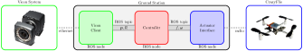
Figure 1: Hardware and ROS Nodes

IV-B Experimental Results

The first experimental test is as follows. We choose as desired trajectory a circle on the horizontal plane with radius r = 0.25 m, reference speed norm $\text{v}_{d}=||\boldsymbol{\text{v}}_{d}||=0.1\;\text{m/s}$ and yaw angle $\psi_{d}=0$ along the curve. In order to perform the desired motion, the quadrotor is first controlled in order to hover into a neighborhood of the position $\boldsymbol{p}_{d}(0)=[0.25\;\;0.0\;-1.0]^{T}\;\text{m}$, using a standard hovering controller. Then, we switch from the hovering task to the circular motion task, choosing either the trajectory tracking controller or the maneuver regulation one. In order to test the behavior of the system in presence of exogenous disturbances decelerating the vehicle motion and eventually immobilizing it, we operate as follows. During the hovering phase we hold the vehicle and switch from the hovering task to the circular motion task. The vehicle is thus constrained inside a neighborhood of $\boldsymbol{p}_{d}(0)$ with practically zero velocity and completely released after few seconds. This scenario is tested by using both the trajectory tracking and the maneuver regulation schemes. The results are depicted respectively in the left and right columns of Figure 2.

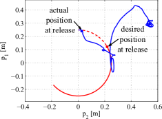
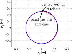
(a) Path $(p_{1},p_{2})$: desired position during holding time (dashed red), desired position after release (solid red), actual position (blue).

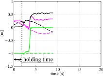
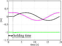
(b) Positions: $p_{1}(t)$ (magenta), $p_{2}(t)$ (black), $p_{3}(t)$ (green); dashed lines are desired positions, while solid lines are actual positions.

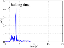
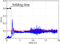
(c) Velocity norm $\text{v}(t)$: desired velocity (red), actual velocity (blue). Note a scale factor of 10 regarding the ordinate axis.

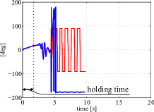
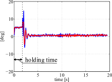
(d) Roll angle $\varphi(t)$: roll angle command (red), actual angle (blue). Note a scale factor of 10 regarding the ordinate axis.

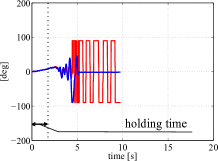
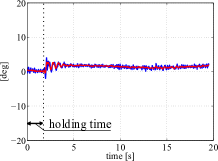
(e) Pitch angle $\theta(t)$: pitch angle command (red), actual angle (blue). Note a scale factor of 10 regarding the ordinate axis.

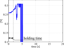
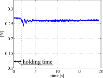
(f) Thrust $f(t)$

Figure 2: Trajectory Tracking (left column) vs Maneuver Regulation (right column).

Let us first analyze the experiment in which the trajectory tracking controller is adopted (left column). During the holding phase, the desired state “keeps moving” thus making the tracking error increase. When the quadrotor is released, the desired position is “far” from the actual position, as depicted in Figure 2a on the left. The vehicle attempts to quickly catch up the reference and this results into the foreseen undesired phenomena. A poor tracking of the desired path is realized: the quadrotor does not track the circular arc, but chooses a shortest path to catch up the position reference. Moreover, the velocity (Figure 2c, left) reaches a peak of more than $4.0$ m/s and the thrust (Figure 2f, left) increases and saturates at the value of $0.31$ N. This behavior causes an instability, as it can be seen from the angles depicted in Figures 2d and 2e (left). The vehicle is not able to recover a controlled motion along the circle and finally falls down. This dangerous behavior is avoided when using the maneuver regulation approach, as shown in Figure 2 (right column). While the quadrotor is constrained, the reference state is suitably chosen according to the actual quadrotor position. Since the reference position is selected as the one on the desired path at minimum distance from the actual position, the position error does not increase. As a consequence, when the quadrotor is released, the maneuver is “smoothly regulated” thus converging to the desired trajectory. Moreover, as it can be noticed in Figure 2c (right), there is just a small velocity overshoot (with a peak of less than $0.3$ m/s) due to a constant velocity error during the constrained phase. The roll and pitch angles (Figures 2d and 2e, right) closely follow the reference, and the thrust (Figure 2f, right) does not increase.

In order to further test the robustness of the maneuver regulation scheme under disturbances, we perform a second experiment. We choose, as desired trajectory, a 90 degree turn with reference speed norm $\text{v}_{d}=0.2\;\text{m/s}$ and yaw angle $\psi_{d}=0$. The quadrotor, controlled using our maneuver regulation control law, is forced to execute the task when linked to a small cardboard box through a nylon thread. Corresponding results are depicted in Figure 3. During a take off maneuver, the vehicle reaches the position $\boldsymbol{p}_{d}(0)=[0.5\;\;0.0\;-1.0]^{T}\text{m}$: the quadrotor is linked to the payload through the thread, but there is no traction through the cable during this phase. After the take off phase, we switch to the desired motion task. As soon as the quadrotor starts moving closely to the desired trajectory, it slows down, affected by the presence of the payload. The vehicle drags the payload through the thread during all its motion. As a consequence, the motion of the vehicle is decelerated with respect to the desired velocity reference, as shown in Figure 3d. Nevertheless, the maneuver regulation controller is still able to stabilize the vehicle, which closely follows the desired path, as depicted in Figure 3a.

(a) Path $(p_{1},p_{2})$: desired position (red), actual position (blue).

(b) Thrust $f(t)$

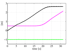
(c) Positions: $p_{1}(t)$ (magenta), $p_{2}(t)$ (black), $p_{3}(t)$ (green); dashed lines are desired positions, while solid lines are actual positions.

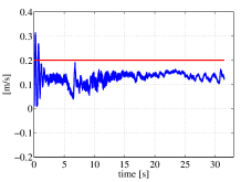
(d) Velocity norm $\text{v}(t)$: desired velocity (red), actual velocity (blue).

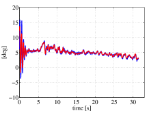
(e) Roll angle $\varphi(t)$: roll angle command (red), actual angle (blue).

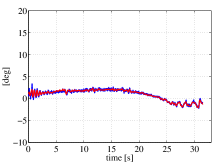
(f) Pitch angle $\theta(t)$: pitch angle command (red), actual angle (blue).

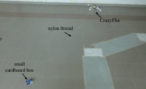
(g) Experimental scenario

Figure 3: Maneuver regulation controller: the vehicle performs a 90 degree turn while dragging a small payload.

V Conclusions

We have presented an easy-to-design maneuver regulation control strategy for VTOL UAVs obtained by means of a trajectory tracking control robustification. Specifically, we have designed a scheme in which the VTOL is required to stay on a given path with a desired velocity profile, rather than catching up a desired time-parametrized state. Since the maneuver regulation controller is derived from a trajectory tracking control scheme, it inherits its properties (while gaining the robustness of maneuver regulation) and does not need a new (possibly time-consuming) parameter tuning. To demonstrate the appealing features of the proposed controller, we have run experimental tests on a nano-quadrotor. In these experiments, we have highlighted the robustness of maneuver regulation with respect to trajectory tracking and demonstrated the correctness of our approach.

References

- [1] C. Powers, D. Mellinger, A. Kushleyev, B. Kothmann, and V. Kumar, “Influence of aerodynamics and proximity effects in quadrotor flight,” in Experimental Robotics, ser. Springer Tracts in Advanced Robotics, J. P. Desai, G. Dudek, O. Khatib, and V. Kumar, Eds. Springer International Publishing, 2013, vol. 88, pp. 289–302.
- [2] M. Furci, G. Casadei, R. Naldi, R. Sanfelice, and L. Marconi, “An open-source architecture for control and coordination of a swarm of micro-quadrotors,” in Unmanned Aircraft Systems (ICUAS), 2015 International Conference on, June 2015, pp. 139–146.
- [3] A. Kushleyev, D. Mellinger, C. Powers, and V. Kumar, “Towards a swarm of agile micro quadrotors,” Autonomous Robots, vol. 35, no. 4, pp. 287–300, 2013.
- [4] A. Roberts and A. Tayebi, “Adaptive position tracking of VTOL UAVs,” Robotics, IEEE Transactions on, vol. 27, no. 1, pp. 129–142, Feb 2011.
- [5] D. Cabecinhas, R. Cunha, and C. Silvestre, “A nonlinear quadrotor trajectory tracking controller with disturbance rejection,” Control Engineering Practice, vol. 26, pp. 1 – 10, 2014.
- [6] ——, “A globally stabilizing path following controller for rotorcraft with wind disturbance rejection,” Control Systems Technology, IEEE Transactions on, vol. 23, no. 2, pp. 708–714, March 2015.
- [7] C. Liu, O. McAree, and W.-H. Chen, “Path following for small uavs in the presence of wind disturbance,” in Control, 2012 UKACC International Conference on, Sept 2012, pp. 613–618.
- [8] G. Antonelli, E. Cataldi, P. Robuffo Giordano, S. Chiaverini, and A. Franchi, “Experimental validation of a new adaptive control for quadrotors,” in 2013 IEEE/RSJ Int. Conf. on Intelligent Robots and Systems, Tokyo, Japan, Nov. 2013, pp. 2439–2444.
- [9] J. Escareño, S. Salazar, H. Romero, and R. Lozano, “Trajectory control of a quadrotor subject to 2D wind disturbances,” Journal of Intelligent & Robotic Systems, vol. 70, no. 1-4, pp. 51–63, 2013.
- [10] P. Castaldi, N. Mimmo, R. Naldi, and L. Marconi, “Robust trajectory tracking for underactuated VTOL aerial vehicles: Extended for adaptive disturbance compensation,” in Proc. of 19–th IFAC World Congress, vol. 19, no. 1, 2014, pp. 3184–3189.
- [11] N. Sydney, B. Smyth, and D. Paley, “Dynamic control of autonomous quadrotor flight in an estimated wind field,” in Decision and Control (CDC), 2013 IEEE 52nd Annual Conference on, Dec 2013, pp. 3609–3616.
- [12] S. Spedicato, G. Notarstefano, H. H. Bülthoff, and A. Franchi, “Aggressive maneuver regulation of a quadrotor UAV,” in 16th Int. Symp. on Robotics Research, ser. Tracts in Advanced Robotics. Singapore: Springer, Dec. 2013.
- [13] J. Hauser and R. Hindman, “Maneuver regulation from trajectory tracking: Feedback linearizable systems,” in Proc. IFAC Symp. Nonlinear Control Systems Design, 1995, pp. 595–600.
- [14] J. Hauser, “Modeling and control of nonlinear systems.” DTIC Document, Tech. Rep., 1996.
- [15] M.-D. Hua, T. Hamel, P. Morin, and C. Samson, “Introduction to feedback control of underactuated VTOL vehicles: A review of basic control design ideas and principles,” Control Systems, IEEE, vol. 33, no. 1, pp. 61–75, Feb 2013.
- [16] V. Mistler, A. Benallegue, and N. M’sirdi, “Exact linearization and noninteracting control of a 4 rotors helicopter via dynamic feedback,” in Proceedings. 10th IEEE International Workshop on Robot and Human Interactive Communication. Bordeaux, Paris, France: IEEE, 2001, pp. 586–593.
- [17] G. Notarstefano, J. Hauser, and R. Frezza, “Computing feasible trajectories for control-constrained systems: the PVTOL example,” in Nolcos, Pretoria, SA, August 2007.
- [18] G. Notarstefano and J. Hauser, “Modeling and Dynamic Exploration of a Tilt-Rotor VTOL aircraft,” in Nolcos, Bologna, Italy, September 2010.
- [19] D. J. Lee, A. Franchi, H. I. Son, H. H. Bülthoff, and P. Robuffo Giordano, “Semi-autonomous haptic teleoperation control architecture of multiple unmanned aerial vehicles,” IEEE/ASME Trans. on Mechatronics, Focused Section on Aerospace Mechatronics, vol. 18, no. 4, pp. 1334–1345, 2013.