Towards a Unified Model of Neutrino-Nucleus Reactions for Neutrino Oscillation Experiments

Abstract

A precise description of neutrino-nucleus reactions will play a key role in addressing fundamental questions such as the leptonic CP violation and the neutrino mass hierarchy through analyzing data from next-generation neutrino oscillation experiments. The neutrino energy relevant to the neutrino-nucleus reactions spans a broad range and, accordingly, the dominant reaction mechanism varies across the energy region from quasi-elastic scattering through nucleon resonance excitations to deep inelastic scattering. This corresponds to transitions of the effective degree of freedom for theoretical description from nucleons through meson-baryon to quarks. The main purpose of this review is to report our recent efforts towards a unified description of the neutrino-nucleus reactions over the wide energy range; recent overall progress in the field is also sketched. Starting with an overview of the current status of neutrino-nucleus scattering experiments, we formulate the cross section to be commonly used for the reactions over all the energy regions. A description of the neutrino-nucleon reactions follows and, in particular, a dynamical coupled-channels model for meson productions in and beyond the $\Delta$(1232) region is discussed in detail. We then discuss the neutrino-nucleus reactions, putting emphasis on our theoretical approaches. We start the discussion with electroweak processes in few-nucleon systems studied with the correlated Gaussian method. Then we describe quasi-elastic scattering with nuclear spectral functions, and meson productions with a $\Delta$-hole model. Nuclear modifications of the parton distribution functions determined through a global analysis are also discussed. Finally, we discuss issues to be addressed for future developments.

KEK-TH-1905, J-PARC-TH-0052

• September 30, 2016

Keywords: neutrino-nucleus interaction, neutrino oscillation

1 Introduction

Extensive researches on reactors, accelerators, solar and atmospheric neutrinos have revealed fundamental properties of the neutrino [1, 2, 3, 4]. Current objectives of neutrino experiments are to precisely determine the neutrino mixing angles and CP violating phase, and to solve the neutrino mass hierarchy problem. Those neutrino properties will be studied with the long-baseline neutrino oscillation experiments such as HK [5, 6] and DUNE [7] near future. To extract the neutrino properties from the neutrino oscillation experiments, one of the major sources of systematic errors is uncertainties in neutrino-nucleus reaction cross sections. Actually, these uncertainties are already one of dominant sources of the systematic errors in the recent neutrino oscillation experiments like T2K. For example, total systematic errors of the number of $\nu_{e}$ and $\bar{\nu_{e}}$ appearance events are ${\cal O}$(6%), and about half of the errors is coming from the uncertainties in the neutrino-nucleus reaction cross sections (Table XX of Ref. [8]; Sec. V​ F​ 3 of Ref. [9]). Therefore, reducing these uncertainties is one of the most important tasks for the currently running and also for the future high precision experiments. Thus a quantitative understanding of the neutrino-nucleus reactions at the level of a few percent accuracy is required to achieve the above-mentioned objectives of the neutrino oscillation experiments [5, 6, 7, 10, 11, 12, 13, 14, 15, 16].

The neutrino energy relevant to the oscillation experiments spans from several hundred MeV to tens of GeV, and thus the neutrino-nucleus reactions over a wide kinematical region need to be understood. From the low to high energy side, the neutrino-nucleus reaction is characterized by the quasi-elastic (QE), resonance (RES), and deep inelastic scattering (DIS) regions (Fig. 1).

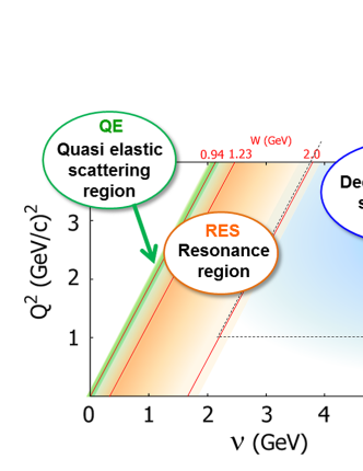
Figure 1: Kinematical regions of the neutrino-nucleus interaction relevant to the next-generation neutrino-oscillation experiments. The energy transfer to a nucleus and the squared four-momentum transfer are denoted by $\nu$ and $Q^{2}$, respectively.

The neutrino-nucleus reactions in each of the regions have quite different characteristics and, accordingly, effective degrees of freedom for theoretical descriptions are quite different. In the QE region, an incident neutrino interacts with one of nucleons inside a nucleus quasi-elastically, and thus nucleons are the effective degrees of freedom. Meanwhile, in the RES region, the internal structure of a scattered nucleon is excited to a resonant state that subsequently decays into a meson-baryon final state; here a meson-baryon dynamics plays a central role. Finally, in the DIS region, a high-energy neutrino even directly sees the subcomponent of the nucleon: the quarks and gluons, or collectively the partons. Perturbative QCD and non-perturbative parton distributions in the nucleon (bound in a nucleus) are basic ingredients for a theoretical description.

Although we roughly divided the kinematical region into three based on the reaction mechanisms, the reality is more complicated. For example, it is well-known that the QE and RES regions overlap to form the so-called ‘dip’ region (the dip between the QE and $\Delta(1232)$ peaks of the nuclear response), and there, processes that involve more than single nucleon (often called two-particle two-hole (2p2h) or $n$-particle $n$-hole ($n$p$n$h) processes) give an important contribution. An example of the 2p2h processes is a process where a pion produced through a $\Delta(1232)$-excitation is absorbed by a surrounding nucleon, leading to a two-nucleon emission. Therefore, in order to understand the dip region, the elementary single nucleon amplitudes for the QE and RES regions should be consistently implemented in a nuclear many-body theory. We also point out that the kinematical region has not necessarily been correctly divided previously. Namely, multi-pion emission rates beyond the $\Delta(1232)$ but still within the (higher-)resonance region have been often estimated with a parton (DIS) model that is extrapolated to the lower $W$ region ($W$: total hadron energy) where the model is in principle not valid. It is important to correctly define the RES and DIS regions considering $W$ and $Q^{2}$, and construct a model suitable for each of the regions.

Obviously, it is essential to combine different areas of expertise to construct ‘a unified model’ for the neutrino-nucleus reactions covering all of the kinematical regions discussed above. Here, ‘a unified model’ does not mean a single theoretical framework that works over all the kinematical region in question. Rather it is constructed by consistently combining baseline models for each of the kinematical regions characterized by the reaction mechanisms, so that transitions between the different kinematical regions can also be well described. In this sense, there already exist several unified models such as neutrino interaction generators (the NEUT [17], the GENIE [18], and the NuWro [19]) that are often used in analyzing data from neutrino experiments. The GiBUU [20] that particularly features a semi-classical hadron transport can also be regarded as a unified model. However, it would be still hoped to develop a new unified model that consists of theoretically and also phenomenologically more well-founded models. Thus, to tackle this issue, experimentalists and theorists recently got together to form a collaboration at the J-PARC Branch of KEK Theory Center [21]. The ultimate goal of this collaboration is to develop a unified model that comprehensively describes the neutrino-nucleus reaction over the QE, RES, and DIS regions. A general outline of our strategy to achieve this goal is the following:

1. We first develop baseline models describing the QE, RES, and DIS regions individually, by applying appropriate physics mechanisms and theoretical treatments, as mentioned above, to each kinematical region.

2. We then connect the hadronic model describing the QE and RES regions to the perturbative QCD model of DIS by matching the cross sections and/or structure functions computed from the two at certain points or region in the ($Q^{2},\nu$) plane, where the transition of the basic degrees of freedom (hadrons versus quarks and gluons) of the reactions is expected to occur.

The purpose and also the unique feature of this article is to report the current status of developing, based on our own approaches, the baseline models for each of the kinematical regions and discuss a future perspective towards a unified neutrino-nucleus reaction model that consists of those baseline models. On the other hand, this article is not intended to comprehensively review all the developments in the field of the neutrino-nucleus reactions on equal footing, although we also cite and sketch other approaches and their recent developments. There exist several review papers on the neutrino-nucleus scattering physics [10, 11, 12, 13, 14, 15, 16] as briefly introduced in the following, and we refer readers to those papers to find more overall developments in the field. Extensive compilation and explanation of existing data for neutrino-nucleon and neutrino-nucleus reactions over the low-energy, QE, RES, and DIS regions are given in Ref. [11]. References [10, 13] particularly focused on the QE processes, summarizing recent theoretical and experimental results, and issues to be resolved. Theoretical approaches to nuclear many-body problems particularly relevant to the QE processes along with the influence of the theoretical treatment on the determination of the neutrino oscillation parameters are discussed in Ref. [14]. Reference [15] discusses neutrino interaction generators and particularly the transport approach GiBUU [20], and their role on the energy reconstruction of incident neutrinos and thus the determination of the neutrino oscillation parameters. References [12, 16] focus on the neutrino interactions on nucleon and nucleus up to a few GeV, putting emphasis on recent developments in the QE-like processes involving multi-nucleon mechanisms; incoherent and coherent meson and photon productions are also discussed.

We spend the rest of this section to describe the organization of this article, and also specify key questions to be addressed in each section.

• We review the current experiments on neutrino-nucleus reactions and the understanding of the data in terms of neutrino reaction generators. Then we summarize open questions and future prospects. These form the introduction of this article.

• We present a cross section formula for neutrino-nucleon(nucleus) reactions for all kinematical regions, and discuss neutrino-nucleon reaction models that are the key building blocks of neutrino-nucleus reaction models. Then we give a dedicated discussion on our recent development of a dynamical coupled-channels model for the whole RES region. There has been a strong demand to develop a model that works well in a region between the $\Delta(1232)$ and the boundary with the DIS where a reliable model has been missing. Such a model should be able to describe the resonant character of the reactions and important two-pion productions. Our development meets this demand. We have achieved, for the first time, to develop a neutrino-nucleon reaction model that fully satisfies the coupled-channels unitarity. The model is constructed from the analysis of pion-, photon- and electron-induced reaction data including multi-meson productions. Comparisons with currently available models are also given.

We then move on to the neutrino-nucleus reactions. Though a main feature of the neutrino-nucleus reactions in the QE, RES and DIS regions can be understood qualitatively from the corresponding elementary processes, an accurate description is very difficult because of the involved nuclear many-body problem. The experience and knowledge on both the reactions and structures of nuclei accumulated in the nuclear physics must be integrated to understand the whole processes of neutrino-nucleus reactions.

• We discuss the low-energy neutrino reactions in few-nucleon systems. This system is particularly attractive as one can describe the nuclear many-body problem accurately with ab initio calculations. A development of the ab initio calculation up to the QE region is highly hoped because it can test, through a comparison with data, meson exchange currents and nuclear correlations in the energy region relevant to the oscillation experiments. The ab initio calculations require a sophisticated technique and experience. Here, we discuss an ab initio approach formulated by a combination of correlated Gaussian and the complex scaling method. Then we report an application of this approach to neutrino-⁴He reactions which has a direct relevance to the neutrino heating in supernova explosions.

• We discuss QE processes. It is well-known that the QE process dominates the cross sections for neutrino reactions on nuclei of $A\ \raise 1.29167pt\hbox{$>$\kern-7.5pt\lower 4.30554pt\hbox{$\sim$}}\$ 10 ($A$: mass number) at the neutrino energies between 0.1 GeV and 1 GeV. A challenge here is to accurately take account of nuclear correlations in the initial and final states. We describe the QE process with the nuclear spectral function and the final state interactions, and show that this approach can provide much better description of data than the conventional Fermi-gas model does.

• We discuss neutrino-nucleus reactions in the RES region. Here, a question is how we microscopically describe hadron dynamics in a nuclear system. We discuss the nuclear effects, such as the rescattering and absorption of pions and the $\Delta$ propagation in nuclei. The rescattering of a produced pion with a spectator nucleon, and the final state interaction between nucleons are examined for the neutrino-deuteron ($\nu$-$d$) reaction. The $\nu$-$d$ reactions play key role to determine the axial vector coupling of the $N\Delta$ transition which is an input for describing the neutrino-nucleus reactions. The pion production reactions in nuclei in the $\Delta$ resonance region have been studied extensively in terms of the $\Delta$-hole approach. As an application of this approach, we discuss neutrino-induced coherent pion-production reactions.

• We discuss neutrino-nucleus reactions in the DIS region. The nuclear medium effects in the DIS region are an interesting and important question. An answer to this question is needed for describing nuclei in terms of quark and gluon degrees of freedom. Also, some previous analyses claimed that the nuclear effects can be different between charged lepton and neutrino DIS. We discuss the current status of the nuclear parton distribution functions from a global analysis of the world data in connection with the neutrino-nucleus reactions. In the region of small $Q^{2}$ and large $\nu$ (see Fig. 1 for the definition of $Q^{2}$ and $\nu$), it is, however, difficult to treat the neutrino-nucleon interaction in terms of perturbative QCD, and thus we will need a help from some other approach such as those based on the Regge phenomenology to describe it. We will briefly summarize such studies, and introduce recent parametrizations for the neutrino reactions. Furthermore, we will also discuss how the Regge region with the small $Q^{2}$ and large $\nu$ could be connected to the regions of DIS and RES.

• We summarize future prospect on how we take an approach towards a unified understanding of the neutrino-nucleus reactions over the wide $W$ and $Q^{2}$ regions.

2 Experimental status

From early 1970’s, neutrino-nucleon/nucleus scatterings were intensively studied with bubble chambers. The bubble chamber detector provides clear images of the neutrino interactions. The charged particles produced in the detectors are identified efficiently and momentum thresholds of the particles are quite low. Also, these detectors are magnetized and charge and momentum of a particle could be measured by the trajectory. Type of a particle could be identified with the thickness of the trajectory, which corresponds to the energy deposit per unit length. Therefore, it is possible to reconstruct nucleon resonance mass with observed charged pion and proton. On the other hand, detection efficiency of gamma was not so high because of the limited size of the detector and there are some difficulties in differentiating low momentum pions from muons by thickness of the track because the masses of these two particles are quite similar. Also, all the images were scanned manually and thus, statistics is limited. Understandings of the incident neutrino fluxes were not satisfactory compared to the standard today. Still, the data sets from the bubble chamber are valuable because recent experiments use different detectors and thus, characteristics of the detector is completely different. These bubble chamber experiments have measured not only total cross sections but also differential cross sections, for example, $d\sigma/dQ^{2}$, $d\sigma/dW$ and so on. Furthermore, some of the bubble chamber experiments have used the Deuterium target (ANL [22, 23], BNL [24, 25], BEBC [26] and FNAL [27]) and they provide neutrino interaction with quasi-free neutron, which could not be achieved by the other later experiments. The other experiments used heavier gases, like Neon, Propane and Freon. These experiments used wide variety of neutrino beam, ranging from a few hundreds of MeV to several tens of GeV. Therefore, various interactions like quasi-elastic, single pion production and deep inelastic scattering of both charged and neutral currents are studied. There are several other neutrino experiments, which have used high energy neutrino beam to study weak interaction, nuclear structure ( structure function $xF_{3}$ measurements ) or short baseline neutrino oscillations. Among them, CHORUS experiment [28] used the emulsion detector with a calorimeter and a muon spectrometer. The emulsion detector provides precise particle track information even around the vertex. The NOMAD experiments [29] used the low averaged drift chambers as the active target. These experiments provided not only the differential cross sections but also charged hadron multiplicities. These multiplicity information are also useful to understand the neutrino interactions at higher $W$ region. CDHS [30], CCFR [31] and NuTeV [32, 33] used similar detectors but optimized for the beamline of each experiment to measure the total cross sections and differential cross sections to extract the structure function, $xF_{3}$. Results from these experiments are basically well explained by a simple model of neutrino-nucleon or neutrino-nucleus reactions within the statistics and the systematic errors.

In 1999, the K2K experiment, the first long-baseline neutrino oscillation experiment to confirm the atmospheric neutrino oscillation, started data taking and collected neutrino interaction data with the near detectors. They found that the forward going muons are much fewer than expected. This observation was found not only in the 1kt Water Cherenkov detector but also in the scintillating fiber tracker detector (SciFi) [34] and the full active scintillator bar detector (SciBar) [35]. The forward deficit was well explained by increasing the axial coupling parameter ($M_{A}$) for charged current QE (CCQE) and CC resonance production, and also by applying the correction to the parton distribution function suggested by Bodek and Yang [36]. The K2K experiment did not publish the absolute cross section but they have extracted $M_{A}$ by fitting the shape of $d\sigma/dQ^{2}$. The extracted $M_{A}$ value was $\sim$ 20 % larger than the nominal value, $\sim 1.0$ GeV/$c^{2}$ (Fig. 2) [34].

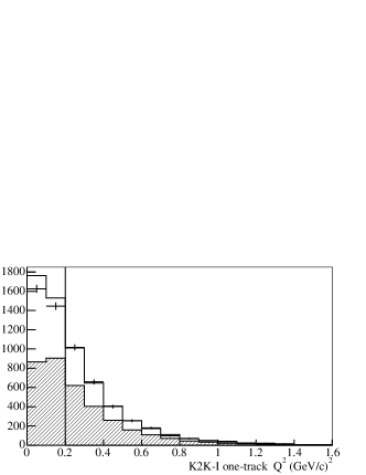
Figure 2: The data and the best fit $Q^{2}_{rec}$ distributions for K2K-1 1 track data (left) and K2K-IIa data (right) from SciFi detector. The shaded region shows the QE fraction of each sample, estimated from the MC. The lowest two data points in each plot are not included in the fit, due to the large uncertainty from various nuclear effects. The best fit value is $M_{A}=$ 1.20 GeV/$c^{2}$ for CCQE. (c) APS [34]

From 2008, the MiniBooNE experiment started publishing the results of various cross section measurements [37, 38]. This experiment utilizes relatively low energy neutrino beam (average $E_{\nu}\sim 0.8$ GeV) and they used the oil Cherenkov detector. They confirmed that the forward going muons are fewer than expected, as observed in K2K. Interestingly, the observed number of CCQE-like events are a few tens of % larger than simple Relativistic Fermi-Gas model prediction. Even after considering the uncertainty of the absolute beam flux, the number of CCQE-like events are significantly larger than the simple model predictions. A similar small $Q^{2}$ deficit was also observed in the MINOS experiment [39] and the best fit $M_{A}$ value is almost the same as the one from the K2K experiment [34].

These results are interesting in various aspects. The forward going muon deficit or small $Q^{2}$ deficit are likely to be due to the inappropriate model for the CCQE reaction on a nucleus and it is necessary to have a more sophisticated model compared to the simple Fermi-Gas model. However, most of the CCQE cross sections from sophisticated models are smaller than those from the simple Fermi-Gas model. On the other hand, the observed results are larger than the Fermi-Gas model gives, and this implies that these analyses may be missing some mechanisms. One of the candidates of the ‘missing’ components is multi-nucleon interactions. These have been observed in the electron-nucleus scattering experiments and thus, it is quite natural to observe them also in the neutrino-nucleus scattering experiments. The MINER$\nu$A experiment tried to identify this kind of interactions [40].

The pion productions via resonance for both nucleon and nucleus target have been studied with the bubble chamber experiments. However, statistics was not sufficient especially for this interaction mode. Then K2K [41] and MiniBooNE [42] experiments measured the neutral-current (NC) $\pi^{0}$ production. The number of events, momentum and angular distributions agree quite well with the expectations and past experiments. On the other hand, CC $\pi^{+}$ production measured in MiniBooNE [43] did not agree with the expectation, and the pion momentum distribution is also different from those from MINER$\nu$A [44]. The source of these differences is not clear and further experimental data are still needed. These differences are expected to be related to the pion re-scattering both in nucleus and in the detector. Therefore, it is crucial to understand not only the initial momentum and directional distributions of pions but also pion interactions. Another interesting topic is the coherent pion production, which is the interaction of neutrino and nucleus without breaking up the nucleus. This interaction produces just lepton and pion in the final state and no nucleons are emitted. Experimentally, this interaction has been studied by searching for the pion + lepton events without nucleon emission. The K2K [35] and SciBooNE [45] experiments found that the cross section of CC coherent pion production in $\sim$ 1 GeV region, is much smaller than the simple PCAC based model [46]. The MINER$\nu$A experiment measured the cross section around a few GeV region, and found them consistent with the recent calculations [47]. The interesting point is that the cross section for the NC coherent pion production was observed to be consistent with the same simple PCAC model in K2K [41] and MiniBooNE [42].

Neutrino-nucleus deep inelastic scattering has been used to determine the structure function $xF_{3}$ and parton distribution functions. In the past experiments, experimental data are corrected and analyzed to determine the structure functions of iso-scalar nucleus or nucleon [30, 31]. Recently, MINER$\nu$A experiment are collecting a large amount of data from 5 GeV to 50 GeV and started studying the partonic nuclear effects [48]. They have observed the deficit in the small $x$ region which is so-called shadowing region. It is important to understand the nuclear dependences of DIS in the experiments where the neutrino beam of this energy range is utilized.

3 Neutrino-nucleon reactions

In this section, we first present a general formula that represents cross section for neutrino-nucleon and neutrino-nucleus reactions for all kinematical regions within the standard model. The cross section formula is written in terms of the structure functions. We will briefly sketch how the structure functions are modeled and evaluated in different kinematical regions such as the QE, RES, and DIS regions. Then we spend a substantial portion of this section to discuss our own work on the dynamical coupled-channels model for the RES region.

3.1 Cross section formula

The charged current (CC) and neutral current(NC) semi-leptonic reactions on a nucleon or on a nucleus are described by the effective interaction from the standard model as

$${\cal L}^{\rm CC} = -\frac{G_{F}}{\sqrt{2}}\frac{m_{W}^{2}}{m_{W}^{2}+Q^{2}}\int d^{4}x[J^{\rm CC}_{\mu}(x)l^{\rm CC\,\mu}(x)+{\rm h.c.}],$$ (1)

$${\cal L}^{\rm NC} = -\frac{G_{F}}{\sqrt{2}}\frac{m_{Z}^{2}}{m_{Z}^{2}+Q^{2}}\int d^{4}xJ^{\rm NC}_{\mu}(x)l^{\rm NC\,\mu}(x),$$ (2)

where $G_{F}$ is the Fermi coupling constant, and $l^{\mu}$ and $J^{\mu}$ are lepton current and quark current, respectively; $m_{W}$ and $m_{Z}$ are the weak boson masses. The quark currents are given as follows,

$$J_{\mu}^{\rm CC}(x) = \bar{u}(x)\gamma_{\mu}(1-\gamma_{5})d^{\prime}(x)+\bar{c}(x)\gamma_{\mu}(1-\gamma_{5})s^{\prime}(x)\ ,$$ (3)

$$J_{\mu}^{\rm NC}(x) = \sum_{q=u,c}\bar{q}\gamma_{\mu}\left(\frac{1}{2}(1-\gamma_{5})-\frac{4}{3}\sin^{2}\theta_{W}\right)q(x)$$ (4)

$$+ \sum_{q=d,s}\bar{q}\gamma_{\mu}\left(-\frac{1}{2}(1-\gamma_{5})+\frac{2}{3}\sin^{2}\theta_{W}\right)q(x)\ ,\,$$

where we kept terms relevant to our following discussions. The weak eigenstates, $d^{\prime}$ and $s^{\prime}$, are written in terms of mass eigenstates and Cabibbo-Kobayashi-Maskawa (CKM) matrix; $\theta_{W}$ is the Weinberg angle. For an analysis of neutrino-nucleus reaction in the QE and RES region, it is convenient to write the quark currents with the vector ($V_{\mu}$) and axial ($A_{\mu}$) currents as,

$$J_{\mu}^{\rm CC}(x) = V_{ud}(V_{\mu}^{+}(x)-A_{\mu}^{+}(x))\ ,$$ (5)

$$J_{\mu}^{\rm NC}(x) = (1-2\sin^{2}\theta_{W})V_{\mu}^{3}(x)-2\sin^{2}\theta_{W}V^{\rm s}_{\mu}(x)-A_{\mu}^{3}(x)$$ (6)

$$= V_{\mu}^{3}(x)-2\sin^{2}\theta_{W}J^{\rm EM}_{\mu}(x)-A_{\mu}^{3}(x)\ ,$$ (7)

where the superscript $+(-)$ indicates the isospin raising (lowering) current, ’3’ is the third component of the isovector, and ’s’ is the isoscalar current; ’${\rm EM}$’ indicates the electromagnetic current. The lepton currents are given as

$$l_{\mu}^{\rm CC}(x) = \sum_{l=e,\mu}\bar{l}(x)\gamma_{\mu}(1-\gamma_{5})\nu_{l}(x),$$ (8)

$$l_{\mu}^{\rm NC}(x) = \sum_{l=e,\mu,\tau}\bar{\nu}_{l}(x)\gamma_{\mu}(1-\gamma_{5})\nu_{l}(x).$$ (9)

./neutrino-nucleon-dis (110,110) l1,l2 r1,r2 fermion,tension=1.0l1,i1,l2 photon,tension=1.0i1,i2 phantom,tension=1.0r1,i2,r2 fermion,tension=0.0r1,i2 (83.0,55.0)(109.0,127.8) (83.0,55.0)(111.0,121.8) (83.0,55.0)(113.0,115.8) (83.0,55.0)(115.0,109.8) (83.0,55.0)(117.0,103.8) (83.0,55.0)(119.0,97.8) shade

Figure 3: The neutrino-nucleon (nucleus) reaction. The participating particles are the initial ($l$) and final ($l^{\prime}$) leptons, and the target ($i$) and final $(f)$ hadrons, and the weak boson ($W^{+}$ or $Z$) is exchanged between the lepton and the hadron. Beside the line for each of the particles, its four-momentum is indicated.

We consider a neutrino-nucleon (neutrino-nucleus) reaction that can be diagrammatically represented in Fig. 3. With a matrix element of the above weak interaction and also with kinematical variables defined in Fig. 3, we can write down the cross section in the laboratory frame as

$$\frac{d\sigma^{\alpha}}{d\Omega_{l^{\prime}}dE_{l^{\prime}}} = \frac{G_{F}^{2}C_{\alpha}^{2}}{8\pi^{2}}\frac{|\bm{p}_{l^{\prime}}|}{|\bm{p}_{l}|}L^{\mu\nu}W^{\alpha}_{\mu\nu},$$ (10)

where $\alpha=$ CC or NC; $Q^{2}=-q^{2}$ and $C_{\alpha}=1/(1+Q^{2}/m_{W}^{2})$ $[C_{\alpha}=1/(1+Q^{2}/m_{Z}^{2})]$ for $\alpha=$ CC [NC]; $L^{\mu\nu}$ and $W^{\mu\nu}$ are the lepton and hadron tensors, respectively. The lepton tensor is written as

$$L^{\mu\nu} = 2[p_{l}^{\mu}p_{l^{\prime}}^{\nu}+p_{l}^{\nu}p_{l^{\prime}}^{\mu}-g^{\mu\nu}((p_{l}\cdot p_{l^{\prime}})-m_{l}m_{l^{\prime}})\pm i\epsilon^{\mu\nu\alpha\beta}p_{l,\alpha}p_{l^{\prime},\beta}],$$ (11)

where $+(-)$ in the last term is for neutrino (anti-neutrino) reactions. The hadron tensor is defined by

$$W_{\mu\nu}^{\alpha} = \bar{\sum_{i}}\sum_{f}(2\pi)^{3}V\frac{E_{T}}{M_{T}}\delta^{(4)}(P+q-p_{f})\langle f|J_{\mu}^{\alpha}(0)|i\rangle\langle f|J_{\nu}^{\alpha}(0)|i\rangle^{*}\ ,$$ (12)

where $V$ is the quantization volume that disappears in final results; $E_{T}$ and $M_{T}$ are the energy and the mass of target hadron; $\bar{\sum}_{i}$ is the average of the spin states of the target hadron; $\langle f|J_{\mu}^{\alpha}(0)|i\rangle$ is a matrix element of the quark currents between hadronic states, $|i\rangle$ and $|f\rangle$. The hadron tensor includes all information of the hadron response to the current $J_{\mu}^{\alpha}$. For an inclusive reaction, the hadron tensor can be expressed using two available vectors, the momentum of the target (with mass $M_{T}$) $P$ and the momentum transfer $q$, as

$$W^{\alpha,\mu\nu} = -g^{\mu\nu}W_{1}^{\alpha}+\frac{W_{2}^{\alpha}}{M_{T}^{2}}P^{\mu}P^{\nu}+i\frac{W_{3}^{\alpha}}{2M_{T}^{2}}\epsilon^{\mu\nu\rho\sigma}P_{\rho}q_{\sigma}$$ (13)

$$+\frac{W_{4}^{\alpha}}{M_{T}^{2}}q^{\mu}q^{\nu}+\frac{W_{5}^{\alpha}}{M_{T}^{2}}(P^{\mu}q^{\nu}+q^{\mu}P^{\nu})+\frac{W_{6}^{\alpha}}{M_{T}^{2}}(P^{\mu}q^{\nu}-q^{\mu}P^{\nu}),$$

where we have introduced six structure functions $W_{i}(\nu,Q^{2})$ where $\nu\equiv p_{l}^{0}-p_{l^{\prime}}^{0}$. Then the neutrino-hadron inclusive reaction cross section for the laboratory frame is given with the structure functions as

$$\frac{d\sigma^{\alpha}}{d\Omega_{l^{\prime}}dE_{l^{\prime}}} =\frac{G_{F}^{2}C_{\alpha}^{2}|\bm{p}_{l^{\prime}}|E_{l^{\prime}}}{2\pi^{2}}\left[2W_{1}^{\alpha}\sin^{2}\frac{\chi}{2}+W_{2}^{\alpha}\cos^{2}\frac{\chi}{2}\right.$$

$$\pm\frac{W_{3}^{\alpha}}{M_{T}}\left((E_{l}+E_{l^{\prime}})\sin^{2}\frac{\chi}{2}-\frac{m_{l^{\prime}}^{2}}{2E_{l^{\prime}}}\right)\left.+\frac{m_{l^{\prime}}^{2}}{M_{T}^{2}}W_{4}^{\alpha}\sin^{2}\frac{\chi}{2}-\frac{m_{l^{\prime}}^{2}}{M_{T}E_{l^{\prime}}}W_{5}^{\alpha}\right]\ ,$$

where $\cos\chi=|\bm{p}_{l^{\prime}}|/E_{l^{\prime}}\cos\theta$ with $\theta$ being the lepton scattering angle, and $\pm$ are for neutrino and anti-neutrino reactions, respectively. The contributions of $W_{4}^{\alpha}$ and $W_{5}^{\alpha}$ are proportional to the lepton mass and can be neglected in the high energy reactions. $W_{6}^{\alpha}$ term does not contribute to the cross section. Now the problem is to model and evaluate the structure functions. Depending on $\nu$ and $Q^{2}$, by which a reaction can be categorized into either of QE, RES, or DIS region, the structure functions need to be modelled with different effective degrees of freedom, as we will discuss in the next subsection for neutrino-induced reactions on a single nucleon.

3.1.1 Multipole expansion of structure functions

We introduce standard multipole expansions of weak hadronic current [49, 50]. The Coulomb $T^{JM}_{C}$, electric $T^{JM}_{E}$, longitudinal $T^{JM}_{L}$ and magnetic $T^{JM}_{M}$ multipole operators of the weak hadronic current $J^{\mu}$ are defined as

$$T_{C}^{JM}({J}) = \int d\bm{x}j_{J}(qx)Y_{JM}(\hat{\bm{x}}){J}_{0}(\bm{x}),$$ (15)

$$T_{E}^{JM}({J}) = \frac{1}{q}\int d\bm{x}\bm{\nabla}\times[j_{J}(qx)\bm{Y}_{JJM}(\hat{\bm{x}})]\cdot\bm{{J}}(\bm{x}),$$ (16)

$$T_{M}^{JM}({J}) = \int d\bm{x}j_{J}(qx)\bm{Y}_{JJM}(\hat{\bm{x}})\cdot\bm{{J}}(\bm{x}),$$ (17)

$$T_{L}^{JM}({J}) = \frac{i}{q}\int d\bm{x}\bm{\nabla}[j_{J}(qx)Y_{JM}(\hat{\bm{x}})]\cdot\bm{{J}}(\bm{x}),$$ (18)

where $\bm{Y}_{JLM}(\hat{\bm{x}})$ are vector spherical harmonics.

The structure functions, $W_{1}^{\alpha},W_{2}^{\alpha},W_{3}^{\alpha}$ ($\alpha=$ CC, NC), are expressed using the reduced matrix element between an initial state of angular momentum and parity $J^{\pi}=J_{i}^{\pi_{i}}$ and a final state $J_{f}^{\pi_{f}}$ as

$$2W_{1}^{\alpha} = \sum_{f}\frac{4\pi}{2J_{i}+1}\delta(E_{l}+E_{T}-E_{l^{\prime}}-E_{f})R^{\alpha}_{T},$$ (19)

$$W_{2}^{\alpha} = \sum_{f}\frac{4\pi}{2J_{i}+1}\delta(E_{l}+E_{T}-E_{l^{\prime}}-E_{f})(R^{\alpha}_{L}+\frac{Q^{2}}{2|\bm{q}|^{2}}R^{\alpha}_{T}),$$ (20)

$$\frac{W_{3}^{\alpha}}{M_{T}} = -\sum_{f}\frac{4\pi}{2J_{i}+1}\delta(E_{l}+E_{T}-E_{l^{\prime}}-E_{f})\frac{R^{\alpha}_{T^{\prime}}}{|\bm{q}|},$$ (21)

where $R^{\alpha}_{T}$, $R^{\alpha}_{L}$, and $R^{\alpha}_{T^{\prime}}$ are respectively given as

$$R^{\alpha}_{L} = \sum_{J}|<T^{J}_{C}(J^{\alpha,A})+\frac{\omega}{|\bm{q}|}T^{J}_{L}(J^{\alpha,A})>|^{2}+|\frac{Q^{2}}{|\bm{q}|^{2}}<T^{J}_{C}(J^{\alpha,V})>|^{2},$$ (22)

$$R_{T}^{\alpha} = \sum_{J}\sum_{\beta=M,E}[|<T^{J}_{\beta}(J^{\alpha,V})>|^{2}+|<T^{J}_{\beta}(J^{\alpha,A})>|^{2}],$$ (23)

$$R_{T^{\prime}}^{\alpha} = \sum_{J}2{\rm Re}[<T^{J}_{M}(J^{\alpha,V})><T^{J}_{E}(J^{\alpha,A})>^{*}$$ (24)

$$+<T^{J}_{M}(J^{\alpha,A})><T^{J}_{E}(J^{\alpha,V})>^{*}]\ .$$

$T^{J}(J^{\alpha,V})$ [$T^{J}(J^{\alpha,A})$] denotes multipole operators for the vector [axial] part of the hadron current $J^{\alpha}$ in Eqs. (5)-(6). The reduced matrix element of the multipole operator $<T^{J}>=\left<J_{f}\left\|T^{J}\right\|J_{i}\right>$ is defined as

$$\left<J_{f},M_{f}\left|T^{JM}\right|J_{i},M_{i}\right> = \frac{(J_{i},M_{i},J,M|J_{f},M_{f})}{\sqrt{2J_{f}+1}}\left<J_{f}\left\|T^{J}\right\|J_{i}\right>.$$ (25)

Here the matrix element of the longitudinal multipole operator of the vector current is eliminated in Eq. (22) with the help of the current conservation relation of the vector current, $q\cdot V=0$.

3.2 Neutrino-induced reactions on nucleon in the QE, RES, and DIS regions

For the QE scattering, the response of the nucleon to the weak current is represented by nucleon form factors. The matrix elements of the vector and axial currents evaluated with nucleon states are generally parametrized in terms of the form factors as follows:

$$\langle N(p^{\prime})|V_{\mu}^{\pm}(0)|N(p)\rangle = \bar{u}_{N}(\bm{p}^{\prime})\left[f_{V}(Q^{2})\gamma_{\mu}+i{f_{M}(Q^{2})\over 2m_{N}}\sigma_{\mu\nu}q^{\nu}\right]\tau^{\pm}u_{N}(\bm{p})\ ,$$ (26)

$$\langle N(p^{\prime})|A_{\mu}^{\pm}(0)|N(p)\rangle = \bar{u}_{N}(\bm{p}^{\prime})\left[f_{A}(Q^{2})\gamma_{\mu}\gamma_{5}+f_{P}(Q^{2})\gamma_{5}q_{\mu}\right]\tau^{\pm}u_{N}(\bm{p})\ ,$$ (27)

where we have omitted the second class currents. For a recent investigation of possible effects from the second class current on neutrino-nucleus scatterings, see Ref. [51]. The nucleon spinor with the momentum $\bm{p}$ is denoted by $u_{N}(\bm{p})$ and the isospin spinor, on which the isospin raising (lowering) operator $\tau^{\pm}\equiv(\tau^{1}\pm i\tau^{2})/2$ acts, is also implicitly included. The quantities, $f_{V}(Q^{2})$, $f_{M}(Q^{2})$, $f_{A}(Q^{2})$, and $f_{P}(Q^{2})$ are the form factors, and $m_{N}$ denotes the nucleon mass. The matrix elements of the third component of the isovector currents are obtained by simply replacing $\tau^{\pm}$ with $\tau^{3}/2$. Similarly, the isoscalar current is also parametrized with different form factors as

$$\langle N(p^{\prime})|V_{\mu}^{s}(0)|N(p)\rangle = \bar{u}_{N}(\bm{p}^{\prime})\left[f^{s}_{V}(Q^{2})\gamma_{\mu}+i{f^{s}_{M}(Q^{2})\over 2m_{N}}\sigma_{\mu\nu}q^{\nu}\right]{1\over 2}u_{N}(\bm{p})\ .$$ (28)

The form factors for the vector current are determined by analyzing electron-nucleon scattering data. Regarding the axial current, the axial form factor $f_{A}(Q^{2})$ is conventionally parametrized in a dipole form as

$$f_{A}(Q^{2})=g_{A}\left({1\over 1+Q^{2}/M_{A}^{2}}\right)^{2}\ ,$$ (29)

with $g_{A}$=1.27 determined by the neutron life time [1]. The axial mass $M_{A}$ has been determined either by neutrino-deuteron QE scattering data or by the pion electroproduction data near threshold, and its value has been estimated to be $M_{A}=1.026\pm 0.021$ GeV [52]. The induced pseudoscalar form factor $f_{P}$ is often related to $f_{A}$ by the PCAC relation and the pion-pole dominance. In addition to the above-described currents, the strange component of the nucleon contributes to the NC neutrino nucleus/nucleon reactions. In particular, the strange axial vector current contribution has been investigated [53, 54, 55, 56]. The iso-scalar axial current is parametrized as

$$\langle N(p^{\prime})|A_{\mu}^{s}(0)|N(p)\rangle = \bar{u}_{N}(\bm{p}^{\prime}){1\over 2}f^{\rm s}_{A}(Q^{2})\gamma_{\mu}\gamma_{5}u_{N}(\bm{p})\ ,$$ (30)

with

$$f^{\rm s}_{A}(Q^{2}) = \frac{\Delta s}{(1+Q^{2}/M_{A}^{2})^{2}}\ .$$ (31)

The experimental value of $\Delta s$ is $\sim-0.1$, while lattice QCD and hadron model calculations suggest a smaller magnitude [56]. With the matrix elements of Eqs. (26)-(28), we can construct the hadron tensor of Eq. (12), and also the structure functions $W_{i}^{\alpha}$ in the cross section formula, Eq. (3.1).

In the RES region, the weak current can excite a nucleon to its resonant states ($N^{*}$), which is followed by a deexcitation through meson emissions. The main process of this kind in the neutrino-nucleon scattering is a single-pion production for which the $\Delta(1232)$ resonance gives a dominant contribution. As the nucleon gets excited to a higher resonance beyond $\Delta(1232)$, the double-pion production becomes comparable or even more important than the single pion production. Also, $\eta N$, $K\Lambda$, and $K\Sigma$ are produced with probabilities suppressed by an order of magnitude. In these meson-production processes, the different meson-baryon channels are strongly coupled with each other in the final state interaction.

Theoretical descriptions of these meson production processes can be categorized into two approaches. One is to relate the divergence of the axial current amplitude with the pion-nucleon reaction amplitude via the PCAC relation at $Q^{2}\sim 0$. Because, at $Q^{2}=0$, only $W^{\alpha}_{2}$ among the structure functions gives nonzero contribution and is solely determined by the divergence of the axial current amplitude, the cross section for the neutrino-induced reaction at $Q^{2}=0$ can be written with that of the pion-nucleon reaction. This approach has been taken in Ref. [57]. However, the validity of this approach is limited to very small $Q^{2}$ region, and the extrapolation of the cross sections from $Q^{2}=0$ to finite $Q^{2}$ is difficult to control. Another approach is to model the processes microscopically with hadronic degrees of freedom. A pioneering work has been done by Adler [58] who analyzed the pion production mechanisms with a model based on the dispersion theory for a unified description of weak and electromagnetic pion production reactions. Then several models [59, 60, 61, 62, 63, 64, 65, 66], which we will briefly review later, have been developed so far, and some of them are focused on the $\Delta(1232)$ region because of its important relevance to the oscillation experiments. Recently, three of the present authors developed a dynamical coupled-channels (DCC) model that includes all relevant resonance contributions of $W\leq 2$ GeV, and takes account of $\pi N,\pi\pi N,\eta N,K\Lambda,K\Sigma$ coupled-channels in the hadronic rescattering [67]. We will discuss the DCC model in detail in the following subsection. Key quantities for the hadronic models are form factors analogous to those in Eqs. (26)-(28) but associated with $N$-$N^{*}$ transitions. For example, the $N$-$\Delta(1232)$ transition matrix element is often parametrized as:

$$\langle\Delta(p_{\Delta}\!=\!p\!+\!q)\,|J^{\rm CC}_{\mu}(0)|N(p)\rangle = \bar{u}_{\Delta}^{\alpha}(\bm{p}_{\Delta})\Gamma_{\alpha\mu}\left(p,q\right)T^{\pm}u_{N}(\bm{p}\,)V_{ud}\ ,$$ (32)

where $u_{\Delta}^{\alpha}(\bm{p}_{\Delta})$ and $T^{\pm}$ are the $\Delta$ vector spinor and the isospin transition operator, respectively, and

$$\Gamma_{\alpha\mu}(p,q) = \left[\frac{C_{3}^{V}}{m_{N}}\left(g_{\alpha\mu}\hbox to0.0pt{\hbox to5.00002pt{\hfil$q$\hfil}\hss}/-q_{\alpha}\gamma_{\mu}\right)+\frac{C_{4}^{V}}{m_{N}^{2}}\left(g_{\alpha\mu}q\cdot p_{\Delta}-q_{\alpha}p_{\Delta\,\mu}\right)\right.$$ (33)

$$\left.+\frac{C_{5}^{V}}{m_{N}^{2}}\left(g_{\alpha\mu}q\cdot p-q_{\alpha}p_{\mu}\right)+C_{6}^{V}g_{\mu\alpha}\right]\gamma_{5}+\left[\frac{C_{3}^{A}}{m_{N}}\left(g_{\alpha\mu}\hbox to0.0pt{\hbox to5.00002pt{\hfil$q$\hfil}\hss}/-q_{\alpha}\gamma_{\mu}\right)\right.$$

$$\left.+\frac{C^{A}_{4}}{m_{N}^{2}}\left(g_{\alpha\mu}q\cdot p_{\Delta}-q_{\alpha}p_{\Delta\,\mu}\right)+C_{5}^{A}g_{\alpha\mu}+\frac{C_{6}^{A}}{m_{N}^{2}}q_{\mu}q_{\alpha}\right]\ ,$$

where $C_{i}^{V}$ and $C_{i}^{A}$ ($i=3,4,5,6$) that depend on $Q^{2}$ are vector and axial form factors, respectively. With well-controlled form factors, we can apply the model to the neutrino-induced meson productions of the whole $Q^{2}$ region. The vector form factors can be reasonably determined by analyzing a large amount of data for single-pion photo- and electro-production off the nucleon. The axial form factors are difficult to determine because of the shortage of experimental information. Thus the axial form factors, those associated with $N$-$\Delta(1232)$ transition in particular, have been estimated with quark models [68, 69], chiral perturbation theory [70, 71], and lattice QCD [72]. However, experimental inputs are still very valuable. For the moment, only the axial $N$-$\Delta(1232)$ transition form factors can be constrained by analyzing the deuterium bubble chamber data [25, 73]. In analyzing the data, however, a complication could arise due to a significant effect from the $NN$ final state interaction as pointed out in Ref. [74] and will be discussed in Sec. 6.1; the previous analyses neglected this effect. For the other axial $N$-$N^{*}$ form factors, the PCAC relation to the $\pi NN^{*}$ couplings is conventionally invoked at $Q^{2}=0$, and a certain $Q^{2}$-dependence is assumed.

The DIS region is usually specified by the kinematical conditions, $W^{2}\geq 4$ GeV² and $Q^{2}\geq 1$ GeV², as shown in Fig. 1. However, different boundaries may be taken depending on researchers. For example, there are some people to take lower $W^{2}$ (e.g. $W^{2}\geq 3.5$ GeV²), and higher $Q^{2}$ values (e.g. $Q^{2}\geq 4$ GeV²) could be taken to avoid higher-twist effects. In the DIS, the Bjorken scaling variable $x$ is used instead of the energy transfer $\nu$, and it is defined by $x=Q^{2}/(2p\cdot q)=Q^{2}/(2m_{N}\nu)$. Furthermore, the structure functions $F_{1}$, $F_{2}$, and $F_{3}$ are usually used instead of $W_{1}$, $W_{2}$, and $W_{3}$ defined in the hadron tensor of Eq. (13), and they are given by

$$\!\!\!\!\!\!\!\!\!\!\!\!\!\!\!\!\!\!\!\!\!\!\!\!\!\!\!\!\!\!\!\!\!\!\!F_{1}^{\,\alpha}(x,Q^{2})=m_{N}W_{1}^{\,\alpha}(\nu,Q^{2}),\ F_{2}^{\,\alpha}(x,Q^{2})=\nu W_{2}^{\,\alpha}(\nu,Q^{2}),\ F_{3}^{\,\alpha}(x,Q^{2})=\nu W_{3}^{\,\alpha}(\nu,Q^{2}).$$ (34)

./neutrino-quark (110,110) l1,l2 r1,r2 fermionl1,i1,l2 photon,tension=1.0i1,i2 fermionr1,i2,r2

If $Q^{2}$ is large, the neutrino-nucleon DIS cross section is described by the simple addition of the $W$ or $Z$ interaction cross sections with individual partons ($i$): $d\sigma(\nu N)=\sum_{i}d\sigma(\nu\,i)$ as shown in Fig. 4. It is called impulse or incoherent assumption, which is valid in the DIS region by considering that partons do not interact with each other, namely frozen, when the $W$ or $Z$ interact with a quark. By this parton model, the structure functions are expressed in the leading order (LO) of $\alpha_{s}$ and also in the leading twist as [75, 76]

$$2xF_{1}^{\,\alpha}(x,Q^{2})_{\rm LO} =F_{2}^{\,\alpha}(x,Q^{2})_{\rm LO},$$ (35)

$$F_{2}^{\,\text{CC}(\nu p)}(x,Q^{2})_{\rm LO} =2x\left[\,d(x,Q^{2})+s(x,Q^{2})+\bar{u}(x,Q^{2})+\bar{c}(x,Q^{2})\,\right],$$ (36)

$$xF_{3}^{\,\text{CC}(\nu p)}(x,Q^{2})_{\rm LO} =2x\left[\,d(x,Q^{2})+s(x,Q^{2})-\bar{u}(x,Q^{2})-\bar{c}(x,Q^{2})\,\right],$$ (37)

$$F_{2}^{\,\text{NC}(\nu p)}(x,Q^{2})_{\rm LO} =x\left[\,\left\{(g_{V}^{u})^{2}+(g_{A}^{u})^{2}\right\}\right.\left\{u^{+}(x,Q^{2})+c^{+}(x,Q^{2})\right\}$$

$$\ \ \ \,\,\,\left.+\left\{(g_{V}^{d})^{2}+(g_{A}^{d})^{2}\right\}\left\{d^{+}(x,Q^{2})+s^{+}(x,Q^{2})\right\}\,\right],$$ (38)

$$xF_{3}^{\,\text{NC}(\nu p)}(x,Q^{2})_{\rm LO} =2x\left[\,g_{V}^{u}\,g_{A}^{u}\left\{u^{-}(x,Q^{2})+c^{-}(x,Q^{2})\right\}\right.$$

$$\ \ \ \ \ \ \left.+\,g_{V}^{d}\,g_{A}^{d}\left\{d^{-}(x,Q^{2})+s^{-}(x,Q^{2})\right\}\,\right].$$ (39)

Here, the parton distribution functions (PDFs) are denoted by $q(x,Q^{2})$ and $\bar{q}(x,Q^{2})$ ($q=u,d,s,c$), and $q^{\pm}$ are given by $q^{\pm}(x,Q^{2})\equiv q(x,Q^{2})\pm\bar{q}(x,Q^{2})$, so that the $q^{-}$ distributions are valence-quark distributions by definition. The strange and charm valence-quark distributions are considered to be small $|s^{-}|,\,|c^{-}|\ll|u^{-}|,\,|d^{-}|$, so that they are usually neglected. There is some indication on $s_{v}(x)\equiv s^{-}(x)\neq 0$ from opposite-sign dimuon production in neutrino reactions; however, its measurements are not accurate enough to determine the distribution. Here, the couplings of neutral-current interactions are given by $g_{V}^{\,q}=T_{q}^{\,3}-2e_{q}\sin^{2}\theta_{W}$ and $g_{A}^{\,q}=T_{q}^{\,3}$ by the third component of the isospin $T_{q}^{3}$ and the quark charge $e_{q}$. The bottom quark contributions are neglected in the expressions, and they can be included by replacing $s(x,Q^{2})$ by $s(x,Q^{2})+b(x,Q^{2})$. The structure functions in the antineutrino reaction, $F_{2}^{\,\text{CC}(\bar{\nu}p)}(x,Q^{2})_{\rm LO}$ and $F_{3}^{\,\text{CC}(\bar{\nu}p)}(x,Q^{2})_{\rm LO}$, can be obtained by the changes, $d\to u$, $s\to c$, $\bar{u}\to\bar{d}$, and $\bar{c}\to\bar{s}$ in Eqs. (36)-(39).

By including higher-order $\alpha_{s}$ effects, we have the expressions

$$\bar{F}_{n}^{\,\alpha}(x,Q^{2}) =C_{n}^{q}(x,Q^{2})\otimes\bar{F}_{n}^{\,\alpha}(x,Q^{2})_{\rm LO}+C_{n}^{g}(x,Q^{2})\otimes xg(x,Q^{2}),$$

$$\bar{F}_{1} =xF_{1},\ \ \bar{F}_{2}=F_{2},\ \ \bar{F}_{3}=xF_{3},$$ (40)

in terms of the coefficient functions $C_{n}^{q}(x,Q^{2})$ and $C_{n}^{g}(x,Q^{2})$, and the symbol $\otimes$ indicates the convolution integral $f(x)\otimes g(x)=\int_{x}^{1}(dy/y)f(x/y)g(y)$. Explicit expressions of the coefficient functions are, for example, found in Ref. [76]. Neutrino scattering measurements have been done often at a relatively low-energy scale of $Q^{2}\sim 1$ GeV², where higher-twist effects could be conspicuous. Considering such effects in the form of longitudinal-transverse structure function ratio $R\equiv F_{L}/(2xF_{1})=\left[(1+4m_{N}^{2}x^{2}/Q^{2})F_{2}-2xF_{1}\right]/(2xF_{1})$, we express $F_{1}$ in terms of $R$ and $F_{2}$ as

$$2xF_{1}(x,Q^{2})=\frac{1+4m_{N}^{2}x^{2}/Q^{2}}{1+R(x,Q^{2})}F_{2}(x,Q^{2}).$$ (41)

In handling the small $Q^{2}$ ($\sim 1$ GeV²) data, Eq. (41) is usually used with the structure function $F_{2}$, which is calculated in terms of the PDFs, by Eq. (40) together with Eqs. (36) and (38). The function $R(x,Q^{2})$ is known in charged-lepton DIS [77], and the same function is often used also in neutrino DIS. Using these structure functions with appropriate PDFs, we can calculate the neutrino-nucleon or nucleus cross sections. In the neutrino-nucleon case, the nucleonic PDFs [78] should be used in calculating the structure functions, whereas the neutrino-nucleus cross sections can be calculated simply by replacing the nucleonic PDFs with the nuclear parton distribution functions (NPDFs). The NPDFs are modified from the corresponding nucleonic PDFs, and the modifications are discussed in Sec. 7.

3.3 Dynamical coupled-channels model for neutrino-induced meson productions

In this subsection, we mainly discuss our own work on a dynamical coupled-channels (DCC) model for neutrino-induced meson productions off the nucleon. First, we briefly review previous microscopic models for the pion productions. Next, we present an overall picture of the DCC model without going into detailed expressions and equations. For a full presentation of the DCC model used for the neutrino reactions, see Refs. [67, 79]. Then we present some selected results from our DCC model-based analysis of $\pi N,\gamma^{(*)}N\to\pi N,\pi\pi N,\eta N,K\Lambda,K\Sigma$ reactions data. Through the analysis, all model parameters that govern hadronic interactions and vector form factors are determined. The $\pi NN^{*}$ couplings are related to the axial $N$-$N^{*}$ transition strength at $Q^{2}$=0 through the PCAC relation. Thus most of parameters needed to calculate the neutrino-induced processes are determined through the analysis. Because of the scarce neutrino data, it is important to have the analysis done before applying the DCC model to the neutrino reactions. With the parameters determined in the analysis and an assumed $Q^{2}$ dependence of the axial form factors, we predict cross sections for the neutrino-induced meson productions that are compared with available experimental data.

3.3.1 Microscopic models for neutrino-nucleon reactions in the RES region

The previous models for the resonance region can be classified into three categories depending on dynamical contents included in the models. Models of the first category consist of a sum of the Breit-Wigner amplitudes that represent resonant contributions. A recent model of this category is found in Ref. [59] where $\Delta(1232)3/2^{+}$, $N(1535)1/2^{-}$, $N(1440)1/2^{+}$ and $N(1520)3/2^{-}$ resonances are considered. Models of the second category consider tree-level non-resonant mechanisms along with resonant ones of the Breit-Wigner type, and are developed in Refs. [60, 61, 62, 63]. The authors of these references considered tree-level non-resonant mechanisms derived from a chiral Lagrangian in addition to $\Delta(1232)$ of the Breit-Wigner type. A more extended model in the second category was developed in Ref. [64] where all 4-star resonances with masses below 1.8 GeV and rather phenomenological non-resonant contributions were considered. The so-called Rein-Sehgal model [80, 81], which has been often used in analyzing data from neutrino experiments, also belongs to the second category, and includes higher resonances whose axial-vector couplings had been estimated with a quark model. In the third category, a model further takes account of the hadronic rescattering, thereby maintaining the unitarity of amplitudes. Such a model in the $\Delta(1232)$ region was developed in Refs. [65, 66]. The DCC model discussed below can be regarded as an extension of the model of Refs. [65, 66]; the Fock space of the $\pi N$ channel is extended to include more hadronic two-body and $\pi\pi N$ channels and higher resonances beyond $\Delta(1232)$.

3.3.2 Overview of Dynamical Coupled-Channels model

The starting point of the DCC model is a set of phenomenological Lagrangians giving interactions among mesons, baryons and external currents. Couplings of the octet pseudoscalar mesons are consistent with those from a chiral Lagrangian at the low-energy limit. We derive a set of meson-baryon interaction potentials, acting on a given Fock space, from the Lagrangians using a unitary transformation method [82, 83]. The potentials obtained in this way are energy independent, and thus unitary amplitudes can be calculated in a straightforward manner. For our particular model, we choose the Fock space that consists of meson-baryon states ($\pi N,\eta N,K\Lambda,K\Sigma$ and $\pi\pi N$ states) and ’bare’ excited states ($N^{*},\Delta,\rho,\sigma$). The bare $N^{*}$ state represents a quark core component of a nucleon resonance of a given spin-parity, and is dressed by the meson cloud to form the resonance. Now our Hamiltonian reads

$$H = H_{0}+v+\Gamma\ ,$$ (42)

where $H_{0}$ is the free Hamiltonian of mesons and baryons, and $v$ is non-resonant interaction potentials between two-body meson-baryon states and also between $\pi\pi$ states. The non-resonant interactions are from $s$-, $t$-, and $u$-channel hadron-exchange and contact mechanisms. $\Gamma$ describes a transition between the bare excited states and two-body states such as $\Delta\leftrightarrow\pi N$ and $\rho\to\pi\pi$. With this Hamiltonian, we solve the coupled-channels Lippmann-Schwinger equation that reads as

$$T_{\beta\alpha}(\bm{p}^{\prime},\bm{p};W) = V_{\beta\alpha}(\bm{p}^{\prime},\bm{p})$$ (43)

$$+\sum_{\gamma}\int d\bar{\bm{p}}\;V_{\beta\gamma}(\bm{p}^{\prime},\bar{\bm{p}})\;G_{\gamma}(\bar{\bm{p}},W)\;T_{\gamma\alpha}(\bar{\bm{p}},\bm{p};W)\ ,$$

where each of the indices $\alpha$, $\beta$, and $\gamma$ specifies one of the channels included in the Fock space. The scattering amplitude ($T$-matrix element) is denoted by $T_{\beta\alpha}$ and the Green’s function for a channel $\gamma$ by $G_{\gamma}$. The interaction potential $V_{\beta\alpha}$ is either $v_{\beta\alpha}$ or $\Gamma_{\beta\alpha}$ in Eq. (42). As mentioned above, thanks to the energy-independent potential $V_{\beta\alpha}$, it is easily proved that the scattering amplitude $T_{\beta\alpha}$ satisfies the multichannel unitarity. The quantity $W$ is the total energy of the hadronic system while $\bm{p}$ and $\bm{p}^{\prime}$ are the incoming and outgoing momenta; for $\pi\pi N$ channels, it is understood that $\bm{p}$ implicitly denotes two independent momenta. Observables such as cross sections for meson-baryon scattering are calculated with the scattering amplitudes in a straightforward manner.

Now let us move on to electroweak processes on a single nucleon. We again use the unitary transformation method to derive electroweak interaction potentials from the Lagrangians that have couplings of external currents to hadrons. Then we describe the electroweak processes with these perturbative potentials followed by hadronic rescattering; the rescattering is described by the scattering amplitudes from Eq. (43). Thus, the electroweak amplitudes are given by

$$A_{\alpha\lambda}(\bm{p}^{\prime},\bm{q};W,Q^{2}) = j_{\alpha\lambda}(\bm{p}^{\prime},\bm{q},Q^{2})$$ (44)

$$+ \sum_{\gamma}\int d\bar{\bm{p}}\;T_{\alpha\gamma}(\bm{p}^{\prime},\bar{\bm{p}};W)G_{\gamma}(\bar{\bm{p}},W)\;j_{\gamma\lambda}(\bar{\bm{p}},\bm{q},Q^{2})\ ,$$

where the index $\lambda$ specifies either of $\gamma^{(*)}N$, $W^{\pm}N$, or $ZN$ channels with a certain polarization, $\bm{q}$ is the momentum brought into the hadronic system from the current. The electroweak interaction potentials are denoted by $j_{\alpha\lambda}$. The electroweak amplitude denoted by $A_{\alpha\lambda}$ corresponds to $\langle f|J^{\mu}_{\alpha}(0)|i\rangle$ in Eq. (12), and thus we can easily see the connection between $A_{\alpha\lambda}$ and the cross section formula of Eq. (3.1) for the neutrino-induced meson productions. Some diagrams with which $A_{\alpha\lambda}$ is build up are shown in Fig. 5.

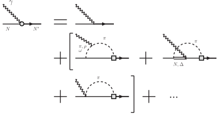
Figure 5: Dressed $\gamma N\to N^{*}$ vertex diagrams. Figure taken from Ref. [67]. Copyright (2015) APS.

3.3.3 DCC analysis of data for pion, photon, and electron-induced meson productions off the nucleon

We have performed a combined analysis of $\pi N,\gamma p\to\pi N,\eta N,K\Lambda,K\Sigma$ reaction data with the DCC model up to $W\leq$ 2.1 GeV (up to $W\leq 2.3$ GeV for $\pi N\to\pi N$) [79]. With suitably adjusted model parameters, the DCC model is able to give reasonable fits to $\sim$23,000 data points. For an extensive presentation of the DCC-based description of the data, see Ref. [79]. The model parameters associated with the hadronic interactions and the vector $N$-$N^{*}$ transition strengths at $Q^{2}=0$ have been fixed through the combined analysis. The DCC model obtained above was also applied to $\pi N\to\pi\pi N$ reactions, and the model predictions were found to give a reasonable description of the data [84]. Before applying the DCC model to the neutrino-induced reactions, we need to determine the $Q^{2}$ dependence of the vector form factors associated with $N$-$N^{*}$ transitions, and also need to separate the vector form factors into isovector and isoscalar parts. The $Q^{2}$ dependence can be determined by analyzing electron-induced reaction data. For the isospin separation, we need to analyze data for photon and electron-induced reactions on the neutron. We have done these analyses to determine the vector form factors for $W\leq$ 2 GeV and $Q^{2}\leq$ 3 GeV² [67]. This covers the whole kinematical region appearing in the neutrino reactions for $E_{\nu}\leq$ 2 GeV.

Figure 6: (Color online) The virtual photon cross section $d\sigma_{T}/d\Omega^{*}_{\pi}+\epsilon\,d\sigma_{L}/d\Omega^{*}_{\pi}$ ($\mu$b/sr) at $Q^{2}$=0.40 GeV² for $p(e,e^{\prime}\pi^{0})p$ from the DCC model. The number in each panel indicates $W$ (MeV). The data are from Ref. [85]. Figure taken from Ref. [67]. Copyright (2015) APS.

Here we present some selected results from the DCC analysis. In Fig. 6, we present the virtual photon cross sections at $Q^{2}$=0.40 GeV² for $p(e,e^{\prime}\pi^{0})p$ from the DCC model in comparison with the data. The agreement with the data is reasonable.

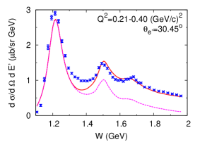
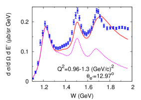
Figure 7: (Color online) Comparison of DCC-based calculation with data for inclusive electron-proton scattering at $E_{e}$=5.498 GeV. The red solid curves are for inclusive cross sections while the magenta dashed-curves are for contributions from the $\pi N$ final states. The range of $Q^{2}$ and the electron scattering angle ($\theta_{e^{\prime}}$) are indicated in each panel. The data are from Ref. [86]. Figures taken from Ref. [67]. Copyright (2015) APS.

Next we present in Fig. 7 differential cross sections for the inclusive electron scattering from the DCC model, and compare them with the data. In the same figure, we also present the single pion electroproduction cross sections from the DCC model. The range of $Q^{2}$ is indicated in each of the panels, and $Q^{2}$ monotonically decreases as $W$ increases. Overall, we see a reasonable agreement between the DCC model with the data. Also, contributions from the multi-pion production processes are increasing above the $\Delta(1232)$ resonance region. We however find a discrepancy between the model and data in $W=1.3\sim 1.45$ GeV at $Q^{2}\sim$ 0.3 GeV². Because the DCC model reasonably describes the single pion electroproduction data as seen in Fig. 6, the discrepancy seems to be from a problem of the model in describing double-pion electroproduction in this kinematics, which might call for a combined analysis including double-pion production data. Our purpose is to develop a neutrino reaction model in the RES region that has a comparable quality to neutrino scattering data that are available in the near future. For this purpose, we believe that the quality of the fits to the electron-induced reactions data at the level seen in the figures should be enough.

3.3.4 DCC model for neutrino-induced meson productions off the nucleon

We now apply the DCC model to the neutrino-induced meson productions. Before doing so, we need to fix the remaining unknown piece, the axial current. The nonresonant axial current can be derived from a chiral Lagrangian on which our $\pi N$ interaction potentials are based. By construction, the nonresonant axial current and the $\pi N$ potentials are related by the PCAC relation at $Q^{2}=0$. For the resonant part, namely, the axial $N$-$N^{*}$ transition strengths at $Q^{2}=0$, we relate them to the corresponding $\pi NN^{*}$ couplings via the PCAC relation. The advantage of our approach over the existing models is that we have the $\pi NN^{*}$ couplings from our DCC model, and thus we can uniquely fix not only the axial coupling strengths but also their phases. In this way, we can make the interference between the resonant and nonresonant axial amplitudes under control within the DCC model. The $Q^{2}$ dependences of the axial couplings are difficult to determine because of the lack of experimental information. Here we assume that all of the axial couplings have the same dipole $Q^{2}$ dependence of $1/(1+Q^{2}/M_{A}^{2})^{2}$ with $M_{A}=1.026$ GeV. With this setup, we make predictions for the neutrino-induced meson productions, results of which are presented below.

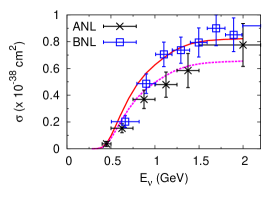
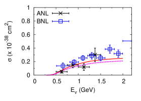
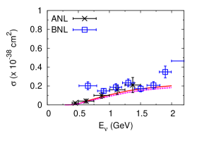
Figure 8: (Color online) The DCC-based calculation (red solid curves) for $\nu_{\mu}\,p\to\mu^{-}\pi^{+}p$ (left), $\nu_{\mu}n\to\mu^{-}\pi^{0}p$ (middle) and $\nu_{\mu}n\to\mu^{-}\pi^{+}n$ (right) in comparison with data. The result obtained with $0.8\times g_{AN\Delta(1232)}^{\rm PCAC}$ is also shown (magenta dashed curve). ANL (BNL) data are from Ref. [73] ([25]). Figures taken from Ref. [67]. Copyright (2015) APS.

We present in Fig. 8 the total cross sections for the single pion productions in comparison with the ANL [73] and BNL [25] data. Our result obtained with the PCAC-based axial $N$-$\Delta(1232)$ transition strength ($g_{AN\Delta(1232)}^{\rm PCAC}$) is consistent with the BNL data for $\nu_{\mu}\,p\to\mu^{-}\pi^{+}p$ (Fig. 8 (left)), and somewhat overestimates the ANL data. For the neutron target processes shown in Fig. 8 (middle, right), our result is consistent with both of the ANL and BNL data. In a recent reanalysis of the ANL and BNL data [87], it was found that the discrepancy between the two datasets can be resolved, and the resulting cross sections are reasonably consistent with the previous ANL data. Therefore, $g_{AN\Delta(1232)}^{\rm PCAC}$ may be too large, and we are tempted to adjust it to fit the ANL data. Thus we present also in Fig. 8 the total cross sections obtained with $g_{AN\Delta(1232)}^{\rm PCAC}$ multiplied by 0.8. Now our cross sections for $\nu_{\mu}\,p\to\mu^{-}\pi^{+}p$ are consistent with the ANL data, and those for $\nu_{\mu}\,n\to\mu^{-}\pi N$ are not largely changed because mechanisms other than the $\Delta(1232)$ excitation are also important for these processes on the neutron target. In our present calculations, we do not consider nuclear effects that must exist in the deuterium target processes. Because Ref. [74] showed a large nuclear effect, it will be important to analyze the deuterium bubble chamber data [23, 25, 73] with the nuclear effects taken into account.

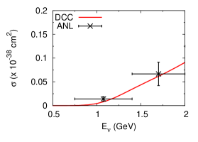
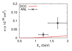
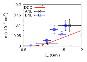
Figure 9: (Color online) The DCC-based calculation for $\nu_{\mu}\,p\to\mu^{-}\pi^{+}\pi^{0}p$ (left), $\nu_{\mu}\,p\to\mu^{-}\pi^{+}\pi^{+}n$ (middle) and $\nu_{\mu}n\to\mu^{-}\pi^{+}\pi^{-}p$ (right) in comparison with data. ANL (BNL) data are from Ref. [88] ([25]). Figures taken from Ref. [67]. Copyright (2015) APS.

We next discuss double pion productions for which our predictions are presented in Fig. 9 in comparison with data [25, 88]. Our calculation for these processes has been done with contributions from all relevant resonances below $W=2$ GeV taken into account for the first time; other previous models [89, 90, 91] consist of dynamical contents that were valid only near the threshold. In comparison with the data, we obtained a good agreement for $\nu_{\mu}\,p\to\mu^{-}\pi^{+}\pi^{0}p$ and $\nu_{\mu}n\to\mu^{-}\pi^{+}\pi^{-}p$. However, the cross sections for $\nu_{\mu}\,p\to\mu^{-}\pi^{+}\pi^{+}n$ are rather underestimated. Because the statistics of the data is rather limited, we do not attempt to fit our model to the data.

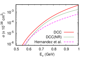
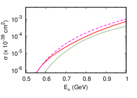
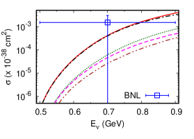
Figure 10: (Color online) Comparison of cross sections from the DCC model with those from the Full model (FF4) of Hernández et al. [91] for $\nu_{\mu}\,p\to\mu^{-}\pi^{+}\pi^{0}p$ (left), $\nu_{\mu}\,p\to\mu^{-}\pi^{+}\pi^{+}n$ (middle) and $\nu_{\mu}n\to\mu^{-}\pi^{+}\pi^{-}p$ (right) near the threshold. Contributions from the non-resonant mechanisms are indicated by ’NR’. In the right panel, the black dash-dotted curve is from the NR and the $P_{11}$ resonant contributions of the DCC model, while the brown dash-two-dotted curve is from the NR of Ref. [91]. In the left and middle panels, the results of Ref. [91] includes only the NR contributions because $N(1440)1/2^{+}$, which is the only resonance considered in Ref. [91], does not contributes to these channels. BNL data are from Ref. [25].

We also compare the result from the DCC model with those from Ref. [91] in Fig. 10. The model of Ref. [91] consists of non-resonant mechanisms derived from a chiral Lagrangian, and a resonant mechanism associated with an excitation of the Roper resonance ($N(1440)1/2^{+}$). Because this dynamical content is expected to be valid only near the threshold, we limit the comparison to $E_{\nu}\ \raise 1.29167pt\hbox{$<$\kern-7.5pt\lower 4.30554pt\hbox{$\sim$}}\ 1$ GeV. For a detailed comparison, non-resonant contributions from the two models are also shown. In $\nu_{\mu}\,p\to\mu^{-}\pi^{+}\pi^{0}p$ (Fig. 10 (left)) and $\nu_{\mu}\,p\to\mu^{-}\pi^{+}\pi^{+}n$ (Fig. 10 (middle)) processes, where $I=1/2$ ($I$: isospin) resonances (and thus the Roper) are not excited, only the non-resonant mechanisms contribute in the model of Ref. [91]. The non-resonant mechanisms of the two models give rather different contributions to each of the channels, but it is difficult to identify the origin of the difference from this comparison only. The resonant contributions are also quite different between the two models. While the Roper resonance in the model of Ref. [91] enhances the $\nu_{\mu}n\to\mu^{-}\pi^{+}\pi^{-}p$ cross sections by $\sim$ 20 - 30 % (Fig. 10 (right)), the contribution seems much smaller than that from the DCC’s resonant $P_{11}$ partial wave amplitude where the Roper exists. The $I=3/2$ resonances, not considered in Ref. [91] but in the DCC model, also give significant contributions as seen in Fig. 10(left,middle) even near the threshold.

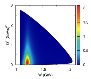
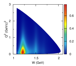
Figure 11: (Color online) $d\sigma/dWdQ^{2}$ for $\nu_{\mu}\,p\to\mu^{-}\pi^{+}p$ (left) and $\nu_{\mu}n\to\mu^{-}\pi N$ (right) at $E_{\nu}=2$ GeV in contour plots. Figures taken from Ref. [67]. Copyright (2015) APS.

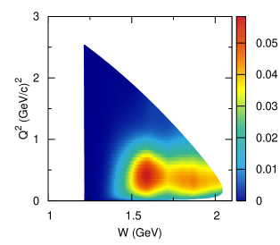
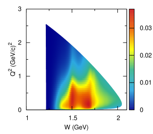
Figure 12: (Color online) $d\sigma/dWdQ^{2}$ for $\nu_{\mu}\,p\to\mu^{-}\pi^{+}\pi^{0}p$ (left) and $\nu_{\mu}n\to\mu^{-}\pi^{+}\pi^{-}p$ (right) at $E_{\nu}=2$ GeV in contour plots. Figures taken from Ref. [67]. Copyright (2015) APS.

Now let us examine the double differential cross sections, $d\sigma/dWdQ^{2}$, shown in Fig. 11 for the single pion productions and in Fig. 12 for the double pion productions at $E_{\nu}$=2 GeV. The figures clearly show the resonant behavior. For the single pion productions, the $\Delta(1232)$ excitation creates the prominent peak, with a long tail toward the higher $Q^{2}$ region. For the neutron target process (Fig. 11 (right)), the second resonances at $W\sim$ 1.5 GeV also create the noticeable peak. For the double pion productions, the situation is completely different. We now do not have the $\Delta(1232)$ peak because it is below the threshold for the double pion productions, and the main contributors are the $N^{*}$s in the so-called second and third resonance regions as clearly seen in Fig. 12.

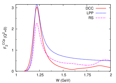
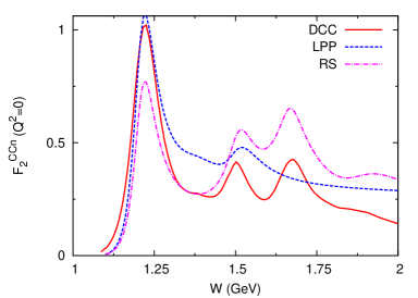
Figure 13: (Color online) $F^{\rm CC}_{2}$ at $Q^{2}=0$ for the single pion production. The DCC model is compared with Lalakulich et al. (LPP) model [59] and Rein-Sehgal (RS) model [80, 81]. The left (right) panel is for the CC $\nu_{\mu}\,p$ ($\nu_{\mu}\,n$) reaction. Figures taken from Ref. [67]. Copyright (2015) APS.

Finally, we compare our predictions from the DCC model with those from other models developed by Lalakulich et al. (LPP) [59] and Rein-Sehgal (RS) [80, 81]. The LPP model consists of four Breit-Wigner amplitudes for $\Delta(1232)3/2^{+}$, $N(1535)1/2^{-}$, $N(1440)1/2^{+}$ and $N(1520)3/2^{-}$ resonances with no background. The RS model has 18 Breit-Wigner amplitudes plus a non-interfering non-resonant background of $I=1/2$. We show in Fig. 13 $F^{\rm CC}_{2}$ (see Eq. (34) for definition) at $Q^{2}=0$ that includes contributions from the single pion production only. Near the $\Delta(1232)$ peak, we find a good agreement between the LPP and the DCC models while the RS model makes a significant underestimation. In the higher energy region, both the LPP and RS models rather overestimate the result from the DCC model. According to the PCAC relation, $F^{\rm CC}_{2}$ at $Q^{2}=0$ is related to the $\pi N$ cross sections, and thus is given almost model-independently. Within our DCC model, the axial current satisfies the PCAC relation to the precise $\pi N$ model by construction, and therefore $F^{\rm CC}_{2}$ from the DCC model agree well with those from the $\pi N$ cross sections. On the other hand, the other models did not fully implement this consistency required by the PCAC relation, and as a consequence, we found the difference in $F^{\rm CC}_{2}(Q^{2}=0)$ between the DCC model and the LPP and the RS models.

4 Neutrino reactions in few-nucleon systems

A precise description of neutrino-nucleus reactions especially in the QE region is crucial for analyzing data from the long-baseline neutrino oscillation experiments. A practical theoretical description of the one-nucleon knock-out reaction in the impulse approximation will be discussed in the next section. However, due to a wide energy band of the neutrino flux, reactions somewhat off the QE peak region become relevant for precisely determining the neutrino properties. In this region, nuclear correlations such as two-particle two-hole effects including meson-exchange currents play an important role. Since precise neutrino-nucleus reaction data comparable to electron scattering are not available, further efforts to reduce systematic uncertainties originating from theoretical treatments of nuclear electroweak break-up reactions are highly called for. An ab initio approach would be a promising option in this regard.

In the ab initio approach, nuclear many-body problems are solved in principle ’exactly’, once nuclear interactions such as realistic nucleon-nucleon potential and nuclear currents (impulse and meson-exchange currents) are set. Approaches of this kind have been extensively applied to low-energy ($E_{\nu}\ \raise 1.29167pt\hbox{$<$\kern-7.5pt\lower 4.30554pt\hbox{$\sim$}}\ 100$ MeV) break-up reactions in few-nucleon systems. This is partly because the knowledge of low-energy electroweak processes, neutrino-nucleus reactions in particular, are of great importance to understand astrophysical phenomena such as the neutrino heating in core-collapse supernovae of massive stars [92, 93, 94, 95, 96], nucleosynthesis via neutrino reactions [97, 98], and yields of light isotopes from which the neutrino properties can be extracted [99]. In the next two paragraphs, we briefly summarize previous ab initio calculations for electroweak processes in few-nucleon systems. An extension of these ab initio approaches to higher energy, e.g., the QE peak region, is highly desirable, because it would provide information on the role of nuclear correlations and nuclear currents in the energy region relevant to the neutrino oscillation experiments. Such a calculation for electron scatterings on ⁴He and ¹²C has just been done recently based on the Green’s function Monte Carlo approach, and indeed, leading to interesting findings on those nuclear many-body mechanisms [100]. Yet, it would be desirable to confirm the results with an independent ab initio calculation.

Electroweak reactions in two-nucleon systems at low energies have been studied with the conventional nuclear physics approach (CNPA) that consists of high precision nucleon-nucleon potential and one- and two-nucleon electroweak currents [50, 101]. The approach has been successful in describing electron scattering [102] and photo-reactions [103] with the electromagnetic current, while the nuclear axial vector current has been tested by the muon capture rate [104]. Meanwhile, the effective field theory approach [105], equipped with a systematic expansion scheme, has been applied to the $\nu$-$d$ reaction [106] and recently to the $pp$ fusion reaction [107]. Both approaches agree with each other for the low-energy neutrino-deuteron reactions [101]. Recently, the neutrino-deuteron reaction has been studied up to $E_{\nu}\ \raise 1.29167pt\hbox{$<$\kern-7.5pt\lower 4.30554pt\hbox{$\sim$}}\ 1$ GeV region with the CNPA [108].

Ab initio calculations of electroweak reactions on $A\geq 3$ nuclei including multi-nucleon break-up channels have been carried out with various approaches. Electromagnetic reactions on three-nucleon systems have been extensively studied based on the Faddeev calculations [109]. The Lorentz integral transformation method has been applied to electron scattering and photo reactions [110], and also to neutrino reactions in the supernova environment [111, 112]. The Green’s function Monte Carlo method was used for electromagnetic and NC neutrino reactions [113, 114].

In what follows, we discuss a promising alternative ab initio approach formulated with a combination of the correlated Gaussian (CG) and the complex scaling method (CSM), and its application to the dipole and spin-dipole responses of ⁴He in electroweak processes.

4.1 Calculation of nuclear strength functions

The nuclear excitation processes are described with nuclear strength (response) functions. The nuclear strength functions for the electroweak reactions reflect important information on resonant and continuum structure of the nuclear system. The nuclear strength function with the excitation energy $E$ for an operator ${\mathcal{O}}$ characterized by the angular momentum and isospin labels, $\lambda$ and $p$, is defined by

$$S(p,\lambda,E)=\mathcal{S}_{f\mu}\left|\right<\Psi_{f}|\mathcal{O}_{\lambda\mu}^{p}|\Psi_{0}\left>\right|^{2}\delta(E_{f}-E_{0}-E),$$ (45)

where $\Psi_{0}$ ($\Psi_{f}$) is the ground (final) state wave function with the energy $E_{0}$ ($E_{f}$), and $\mathcal{S}_{f\mu}$ denotes the summation over all the final states as well as the $z$-component of the angular momentum, $\mu$. The label $p$ distinguishes different types of isospin operators, e.g., isoscalar, 1 ($p=$IS), isovector, $\tau_{3}$ ($p=$IV0), charge-exchange $\tau^{\mp}$ ($p=$IV$\mp$), and electric $\frac{1}{2}(1+\tau_{3})$ types ($p=E\lambda$). (Here we adopt convention of isospin described in Sec. 3.2 throughout this paper, while convention in Ref. [115] is $\tau^{+}\left|p\right>=\left|n\right>$ and $\tau_{0}=-\tau_{3}$.) Taking the summation over the final states makes it possible to rewrite the strength function as

$$S(p,\lambda,E)=-\frac{1}{\pi}{\rm Im}\sum_{\mu}\left<\Psi_{0}\right|\mathcal{O}_{\lambda\mu}^{p\dagger}\frac{1}{E-H+E_{0}+i\epsilon}\mathcal{O}_{\lambda\mu}^{p}\left|\Psi_{0}\right>,$$ (46)

where $H$ is the nuclear Hamiltonian and $1/(E-H+E_{0}+i\epsilon)$ is the many-body Green’s function. A positive infinitesimal $\epsilon$ is put to ensure the outgoing wave after the excitation of the initial state.

Though an explicit construction of the final states is avoided in Eq. (46), an evaluation of Eq. (46) is still in general difficult because of the presence of the Green’s function that involves complicated many-body correlations and boundary conditions. We employ the complex scaling method (CSM) [116] to avoid these complications. In the CSM, a particle coordinate (momentum), $\bm{r}$ ($\bm{k}$), is rotated on the complex plane by a positive angle $\theta$ as $\bm{r}{\rm e}^{i\theta}$ ($\bm{k}{\rm e}^{-i\theta}$). Under this transformation, the asymptotics of the wave function damps exponentially at large distances, which allows us to represent the Green’s function in the expansion by the eigenstates of the complex-rotated Hamiltonian, $H(\theta)$,

$$H(\theta)\Psi_{k}(\theta)=E_{k}(\theta)\Psi_{k}(\theta).$$ (47)

This class of complex eigenvalue problems is solved with a set of square-integrable ($\mathcal{L}^{2}$) basis functions. Since the resonant and continuum states are treated in a manner similar to a bound-state problem, the method has widely been applied to calculating the strength functions [117]. The accuracy of the CSM calculation crucially depends on how completely the ${\cal L}^{2}$ basis functions are prepared. In principle, if the model space is complete, the result would not depend on the scaling angle in some limited range of $\theta$. Practically, the $\theta$ value is determined by examining the stability of $S(E)$ against changing $\theta$.

4.1.1 Correlated Gaussian method

As the basis functions we employ correlated Gaussians (CG) [118, 119, 120], which are flexible enough to describe different types of structure and correlated motion of particles. Many examples have confirmed that the CG method can describe, e.g., short-range repulsion and tensor correlations in the nuclear force [120, 121, 122], and both cluster and shell-model configurations [123]. See also a recent review [124]. Because of its flexibility, the basis functions have been applied to describe not only nuclear physics but also other quantum physics [125].

The total wave function with the angular momentum $J$, its $z$-component $M_{J}$, parity $\pi$, and isospin quantum numbers $T,\,M_{T}$ is expressed as a combination of many basis functions. Each basis function is given in $LS$ coupling scheme

$$\Phi_{(LS)JM_{J},TM_{T}}^{\pi}=\mathcal{A}\left[\phi_{L}^{\pi}\times\chi_{S}\right]_{JM_{J}}\eta_{TM_{T}},$$ (48)

where $\mathcal{A}$ is the antisymmetrizer, and the symbol $\left[L\times S\right]_{JM_{J}}$ stands for the angular momentum coupling. The total spin (isospin) function $\chi_{S}$ ($\eta_{T})$ is constructed by a successive coupling of the spin (isospin) functions of all the nucleons.

For the spatial part of the basis function, $\phi_{L}^{\pi}$, we use the CG. Let $\bm{x}$=($\bm{x}_{i}$) denote a set of the Jacobi coordinates excluding the center-of-mass coordinate. We express $\phi_{L}^{\pi}$ as [118, 119]

$$\phi_{LM_{L}}^{\pi}(A,\bm{x})=\exp(-\tilde{\bm{x}}A\bm{x})\theta_{LM_{L}}^{\pi}(\bm{x}),$$ (49)

where $\tilde{\bm{x}}A\bm{x}=\sum_{i,j}A_{ij}\bm{x}_{i}\cdot\bm{x}_{j}$ with a positive-definite symmetric matrix $A$. The angular part $\theta_{LM_{L}}^{\pi}(\bm{x})$ is expressed by coupling the solid harmonics, $\mathcal{Y}_{lm_{l}}(\tilde{u}\bm{x})=|\tilde{u}{\bm{x}}|^{l}Y_{lm_{l}}(\widehat{\tilde{u}\bm{x}})$, where $\tilde{u}\bm{x}=\sum_{i}(u)_{i}\bm{x}_{i}$ is a global vector. The reader is referred to Refs. [119, 120, 126] for details of single-, double-, and triple-global-vector representations. It should be noted that all coordinates are explicitly correlated through the $A$ and $u$ ($u$’s). An advantage of the representation is that it keeps its functional form under any linear transformation of the coordinates, which is a key to describing many-body bound and unbound states in a unified manner.

4.2 Ab initio calculation for ⁴He

4.2.1 Hamiltonian and spectrum of ⁴He

The Hamiltonian of an $N$-nucleon system consists of two- and three-nucleon forces

$$H=\sum_{i=1}^{N}T_{i}-T_{cm}+\sum_{i<j}V_{ij}^{(2)}+\sum_{i<j<k}V_{ijk}^{(3)},$$ (50)

where $T_{i}$ is the single-nucleon kinetic energy and the center-of-mass kinetic energy is subtracted to ensure the nuclear intrinsic motion. We employ Argonne $v$8^′ [127] (AV8^′) potential which contains central, tensor and spin-orbit components. Since it is vital to reproduce the threshold energies in the calculation of the strength function, a central three-body interaction (3NF) [128] is employed to reproduce the binding energies of the three- and four-nucleon bound states.

The ground state wave function of ⁴He is obtained with a superposition of many CG functions of Eq. (48). The set of the variational parameters, $A$, $u$’s, $L$, spin and isospin configurations, are determined by the stochastic variational method (SVM) [119], which allows us to get a precise solution of a many-body Schrödinger equation in a relatively small number of bases. The ground state energy agrees with the one obtained by other methods [120, 121].

The first excited $0^{+}$ and the seven negative-parity states are observed below the excitation energy of 26 MeV [129] and all of them are reproduced very well [130, 131]. It should be noted that the level ordering of ⁴He can be reproduced only when the realistic nuclear interaction is employed. If one uses an effective interaction that consists of a central term alone, the negative parity levels would be almost degenerate, and no correct level ordering could be obtained [131]. The tensor term plays a decisive role, for example, the lowering of $J^{\pi}T=0^{-}0$ state is understood by a strong coupling between different angular momentum channels due to the tensor force [120].

4.2.2 Dipole-type excitations of ⁴He

The dipole- and spin-dipole(SD)-type operators are main pieces to determine neutrino-⁴He reaction cross sections at low energies. Though the SD operators belong to a class of the first forbidden transition, they can dominantly contribute to the reaction on ⁴He because the Fermi and Gamow-Teller type transitions are strongly suppressed due to the closed shell nature.

The spectrum of the four-nucleon system is closely related to the dipole-type electroweak responses. The seven negative-parity states of ⁴He can be excited by six SD and one dipole operators [115]. Basis functions for the final states reached by these operators are constructed by paying attention to two points: the sum rule of the electroweak strength functions and the decay channels [115, 132]. In fact the basis functions are constructed in three types: (i) a single-particle excitation built on the ⁴He ground-state wave function multiplied by $\mathcal{O}_{\lambda\mu}^{p}$. (ii) a $3N$+$N$ (³H+$p$ and ³He+$n$) two-body disintegration. (iii) a $d$+$p$+$n$ three-body disintegration. The basis (i) is useful for satisfying the sum rule, and the bases (ii) and (iii) take care of the two- and three-body decay asymptotics. These cluster configurations are better described using appropriate relevant coordinates rather than the single-particle coordinate. The relative motion between the clusters is described with several Gaussians. For the wave functions of $d$ and $3N$ subsystems, we use a set of the bases obtained by the two- and three-body calculations with the SVM algorithm [118, 119], which greatly reduces the total dimension of the matrix elements. The expression is again given in the CG with the global vectors and the matrix elements can be evaluated without any change of the formulas.

4.2.3 Photoabsorption of ⁴He

First, we discuss photoabsorption reactions of ⁴He to see the reliability of the method. There has been a controversy in the low-lying photoabsorption cross section, that is, the experimental data are in serious disagreement [133, 134]. In the energy region around 26 MeV, the photoabsorption reaction takes place mainly through the electric-dipole ($E1$) transition. The cross section $\sigma_{\gamma}(E_{\gamma})$ can be calculated by the formula [135]

$$\sigma_{\gamma}(E_{\gamma})=\frac{4\pi^{2}}{\hbar c}E_{\gamma}\frac{1}{3}S(E_{\gamma}),$$ (51)

where $S(E)$ is the strength function for the $E1$ transition with the $E1$ operator $\sum_{i}(\bm{\xi}_{i})_{\mu}\frac{1}{2}(1+\tau_{3i})$ where $\bm{\xi}_{i}=\bm{r}_{i}-\bm{x}_{N}$, and $\bm{x}_{N}$ denotes the center-of-mass coordinate of the $N$-nucleon system.

Figure 14 compares the theoretical and experimental photoabsorption cross sections $\sigma_{\gamma}(E_{\gamma})$. The calculation predicts a sharp rise of the cross section from the threshold, which is observed by several measurements [134, 136] but not in the data of Ref. [133]. Our result satisfies almost 100% of the non-energy-weighted sum rule (NEWSR), and this is also consistent with the cross sections obtained by the Lorentz Integral Transform calculations [137, 138], especially in the cross section near the threshold. The low-lying photoabsorption cross sections are mostly understood by the excitation of the $3N+N$ relative motion. In fact, the $3N+N$ contribution dominates in the low-lying $E1$ strength [132]. Thus, it is hard to understand the low-lying behavior of Ref. [133], though all the data are consistent above 30 MeV.

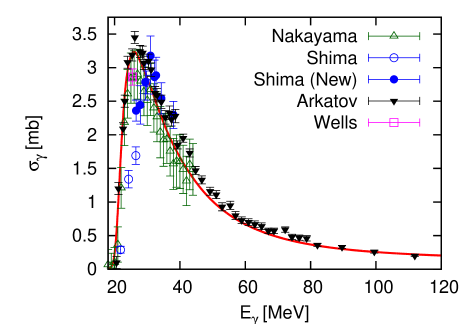
Figure 14: Photoabsorption cross sections of ⁴He obtained with the AV8^′+3NF interaction. The figure is drawn based on the data of Ref. [132]. The experimental data are taken from Refs. [136, 139, 133, 134, 140].

4.2.4 Spin-dipole excitations

We have confirmed the reliability and potential predictive power of our approach. It is interesting to apply it to the SD response of ⁴He because the relevant operators are closely related to those of the neutrino-nucleus reaction. Figure 15 exhibits the SD strength functions of IV$-$ type, $\mathcal{O}_{\lambda\mu}^{{\rm IV}-}=\sum_{i}\left[\bm{\xi}_{i}\times\bm{\sigma}_{i}\right]_{\lambda\mu}\tau^{-}_{i}$, which excites the ground state of ⁴He to the excited states of ⁴H. The NEWSR for the SD operators are fully satisfied, and it is a very interesting observable that can reveal the role of the tensor force in the ground state [115]. The peak positions well correspond to the observed excitation energies of the three negative-parity states of ⁴H [129]. The ratio of the strengths for $J^{\pi}=0^{-}$ ,$1^{-}$, and $2^{-}$ is roughly 1:3:5 following their multipolarity $2J+1$ but the ratio is actually modified to approximately 1:2:4 due to the tensor force [115]. We can also estimate the decay width of the resonance by taking the difference of two excitation energies at which the strength becomes half of the maximum strength at the peak. The agreement between theory and experiment is very satisfactory. The strength functions can also be compared with the spin-flip cross sections of the ⁴He(⁷Li,⁷Be$\gamma$) measurement [134]. Since the absolute value of the SD component was not determined experimentally, the experimental distribution is normalized to the sum of the theoretical strength for $\lambda=0,1,2$ integrated from 18 to 44 MeV where the experimental data are available. The comparison between the theory and experiment is qualitative, but the experimentally observed peak apparently agrees with the calculated one and it is dominated by the $J^{\pi}T=2^{-}1$ state of ⁴H.

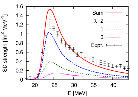
Figure 15: Spin-dipole strength functions of ⁴He to ⁴H charge-exchange process with the AV8^′+3NF interaction. The figure is drawn based on the data of Ref. [115]. The ‘experimental data’ are taken from Ref. [134] for reference. See text for a detail.

4.2.5 Neutrino-⁴He reactions

The typical temperature of the core-collapse supernova is around 10 MeV and the energy of neutrino is rather low $E_{\nu}<100$ MeV. In this energy region below the pion production threshold, the neutrino (anti-neutrino)-⁴He CC and NC reactions lead to the following continuum states:

$$\nu_{e}+{\rm{}^{4}He} \rightarrow e^{-}+3p+n,\ e^{-}+2p+d,\ e^{-}+p+{\rm{}^{3}He}$$ (52)

$$\bar{\nu}_{e}+{\rm{}^{4}He} \rightarrow e^{+}+p+3n,\ e^{+}+2n+d,\ e^{+}+n+{\rm{}^{3}H}$$ (53)

$$\nu+{\rm{}^{4}He} \rightarrow \nu+2p+2n,\ \nu+p+n+d,\ \nu+n+{\rm{}^{3}He},$$ (54)

$$\nu+p+{\rm{}^{3}H},\ \nu+2d$$

The inclusive neutrino-nucleus cross section including all continuum final states can be studied using the strength functions from the ab initio approach.

The transition matrix elements for the low-energy neutrino-⁴He reaction would be dominated by the first-forbidden transitions leading to the negative parity states. The allowed Gamow-Teller and Fermi transitions are expected to be very weak because of the doubly-closed shell structure of ⁴He. In this work, we consider following one nucleon vector and axial vector currents,

$$V_{IA,0}^{\alpha}(\bm{X}) = \sum_{i}f_{V}\tau_{i}^{\alpha V}\delta(\bm{X}-\bm{\xi}_{i}),$$ (55)

$$\bm{A}_{IA}^{\alpha}(\bm{X}) = \sum_{i}f_{A}\bm{\sigma}_{i}\tau_{i}^{\alpha A}\delta(\bm{X}-\bm{\xi}_{i}).$$ (56)

Here the isospin operators are $\tau_{i}^{\alpha V}=\tau_{i}^{\alpha A}=\tau_{i}^{\pm}$ for CC $\nu$ and $\bar{\nu}$ reactions, and $\tau_{i}^{\alpha V}=(1-2\sin^{2}\theta_{W})\tau^{3}/2-2\sin^{2}\theta_{W}$, $\tau_{i}^{\alpha A}=\tau_{i}^{3}/2$ for NC reactions. Here $\theta_{W}$ is Weinberg angle. The one-nucleon operators for the first-forbidden transition in the long wavelength approximation are given as

$$\mathcal{O}_{JM}=\sum_{i}f_{A}[\bm{\xi}_{i}\otimes\bm{\sigma}_{i}]^{J}_{M}\tau^{\alpha A}_{i}$$ (57)

for the axial vector current and

$$\mathcal{O}_{1M}=\sum_{i}f_{V}(\bm{\xi}_{i})_{M}\tau^{\alpha V}_{i}$$ (58)

for the vector current. It is noticed that only $T=1$ states are excited because the isoscalar dipole operator is reduced to the center of mass coordinate.

In the following we focus on the cross section formula of CC reactions. The inclusive cross sections for $\nu/\bar{\nu}$-⁴He CC reactions in the low-energy region are given with the following strength functions $S_{x}(p,J,\omega)$:

$$S_{sd}(p,J,\omega) =\mathcal{S}_{f}|\left<\Psi_{f}\right\|\sum_{j}[\bm{\xi}_{j}\otimes\bm{\sigma}_{j}]_{(J)}\tau^{\pm}_{j}\left\|\Psi_{{\rm{}^{4}He}}\right>|^{2}\delta(E_{f}-E_{0}-\omega),$$ (59)

$$S_{d}(p,1,\omega) =\mathcal{S}_{f}|\left<\Psi_{f}\right\|\sum_{j}\bm{\xi}_{j}\tau^{\pm}_{j}\left\|\Psi_{{\rm{}^{4}He}}\right>|^{2}\delta(E_{f}-E_{0}-\omega),$$ (60)

$$S_{sd-d}(p,1,\omega) =\mathcal{S}_{f}\left<\Psi_{f}\right\|\sum_{j}[\bm{\xi}_{j}\otimes\bm{\sigma}_{j}]_{(1)}\tau^{\pm}_{j}\left\|\Psi_{{\rm{}^{4}He}}\right>\left<\Psi_{f}\right\|\sum_{j^{\prime}}\bm{\xi}_{j^{\prime}}\tau^{\pm}_{j^{\prime}}\left\|\Psi_{{\rm{}^{4}He}}\right>^{*}$$

$$\times\delta(E_{f}-E_{0}-\omega),$$ (61)

where $\omega=E_{\nu}-E_{e}$. The last term $S_{sd-d}(p,1,\omega)$ is the interference term of the vector and axial vector currents. Here $p=$IV$\pm$ for CC neutrino and anti-neutrino reactions. Using the standard multipole expansion formula of neutrino reactions in Sec. 3.1.1, the structure functions $W_{i}$ are given in terms of the strength functions as

$$W_{2} = V_{ud}^{2}\left(W_{L}+\frac{Q^{2}}{2|\bm{q}|^{2}}W_{T}\right),$$ (62)

$$2W_{1} = V_{ud}^{2}\,W_{T},$$ (63)

where

$$W_{T} = f_{A}^{2}|\bm{q}|^{2}\left(\frac{1}{3}S_{sd}(p,1,\omega)+\frac{1}{5}S_{sd}(p,2,\omega)\right)+f_{V}^{2}\frac{2\omega^{2}}{3}S_{d}(p,1,\omega),$$ (64)

$$W_{L} = f_{A}^{2}\omega^{2}\left(\frac{1}{3}S_{sd}(p,0,\omega)+\frac{2}{15}S_{sd}(p,2,\omega)\right)+f_{V}^{2}\frac{Q^{4}}{3|\bm{q}|^{2}}S_{d}(p,1,\omega),$$ (65)

$$\frac{W_{3}}{M_{T}} = \frac{2\sqrt{2}}{3}f_{A}f_{V}\omega S_{sd-d}^{1}(p,1,\omega).$$ (66)

Similar expressions can be obtained for NC reactions.

The cross sections $d\sigma/dE$ of neutrino-⁴He CC (left) and NC (right) reactions as a function of excitation energy ($E$) at $E_{\nu}=50$ MeV are shown in Fig. 16. Here the cross sections are obtained by using the strength functions calculated in Ref. [115]. As shown in Fig. 16, the contributions of spin-dipole operators of $J^{\pi}T=$ $2^{-}1$ and $1^{-}1$ give main strength of the neutrino reactions. The contribution of $0^{-}1$ states is small for both CC and NC reactions, while the dipole operator gives non-negligible contribution for the CC reaction. The energy dependence of the total cross sections for CC $\nu_{e}-^{4}$He, CC $\bar{\nu}_{e}-^{4}$He and NC $\nu_{e}-^{4}$He reactions are shown in Fig. 17. The cross section of the ab initio calculation is shown in solid curve. For comparison, results of shell-model calculation [141] with the WBP [142](green circle) and SPSDMK [143](blue square) shell model interactions are also shown in Fig. 17. The ab initio calculation of NC reaction agrees with the shell model calculation of SPSDMK, while for CC reaction, the $S_{sd-d}$ term, which has not been included in our current calculation, may give a sizable contribution because of non-negligible contribution of the dipole operator; the $S_{sd-d}$ term is the $V$-$A$ interference term in which the matrix elements of the vector current and the axial vector current interfere.

Before predicting the temperature average cross section for the simulation of supernova explosion, we have to include $V$-$A$ interference term for $1^{-}1$ final states, meson-exchange current for the axial vector current and possible contribution of the recoil order term to the time component of the axial vector current $A_{0}\sim\bm{p}\cdot\bm{\sigma}/m_{N}$, which has been studied for the nuclear muon capture reaction [144]. Taking into account those effects, the ab initio study of the neutrino reaction is of great interest to help to clarify the role of light nuclei for the heating mechanism of the core-collapse supernova.

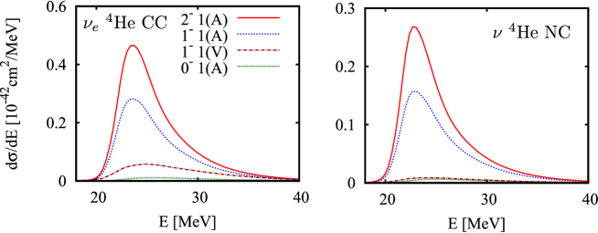
Figure 16: The differential cross sections $d\sigma/dE$ of neutrino-⁴He CC(left) and NC(right) reactions at $E_{\nu}=50$MeV. Contributions of axial vector spin-dipole operators as a function of nuclear excitation energy $E$ are shown in solid (red) ($J^{\pi}T=2^{-}1(A)$), long-dashed (blue) ($1^{-}1(A)$) and short-dashed (green) curves ($0^{-}1(A)$). The contribution of dipole operator of vector current is shown in dash-dotted (brown) ($1^{-}1(V)$) curve.

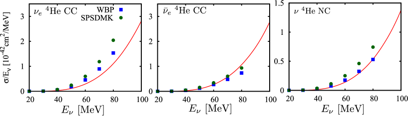
Figure 17: The total cross section of CC reactions ($\nu_{e}+{\rm{}^{4}He}\rightarrow e^{-}+X$ (left panel) and $\bar{\nu}_{e}+{\rm{}^{4}He}\rightarrow e^{+}+X$ (middle panel)) and NC reaction ($\nu+{\rm{}^{4}He}\rightarrow\nu+X$ (right panel)). The solid curves show the result of this work and are compared with the shell model calculation [141] with the WBP(green circle) and SPSDMK(blue squares) shell model interactions.

5 Quasi-Elastic Interactions

As stressed in the Introduction, the next-generation neutrino oscillation experiments that aim at extracting the neutrino-mass hierarchy and leptonic CP violation would require a quantitative understanding of the neutrino-nucleus interactions at the level of a few % accuracy or better. In the neutrino energy region from 0.2 to 2.0 GeV, the charged-current quasi-elastic (CCQE) process gives the largest contributions than the other reaction mechanisms induced by neutrinos. In neutrino oscillation experiments utilizing neutrinos in this energy region, the neutrino energy is often reconstructed using a formula based on the QE kinematics with the initial nucleon at rest as follows:

$$E_{\nu}^{\textrm{Rec}}=\frac{2E_{l^{\prime}}\tilde{m}_{N}-(m_{l^{\prime}}^{2}+\tilde{m}_{N}^{2}-m_{N}^{2})}{2(\tilde{m}_{N}-E_{l^{\prime}}+p_{l^{\prime}}\cos\theta_{l^{\prime}})},$$ (67)

where $\tilde{m}_{N}=m_{N}-\epsilon$ with $\epsilon$ being the separation energy; $E_{l^{\prime}}=\sqrt{p_{l^{\prime}}^{2}+m_{l^{\prime}}^{2}}$. With this formula, the neutrino energy is reconstructed with the final lepton kinematics ($p_{l^{\prime}}$ and $\theta_{l^{\prime}}$) measured in the experiments. However, the relation of Eq. (67) could be considerably modified by the Fermi motion of the initial nucleon and the final state interaction (FSI) of the outgoing nucleon. Therefore, a reliable modeling of the CCQE process is of particular importance to extract precise neutrino flux from the data.

In this section, we describe the inclusive lepton-nucleus reactions in the ’impulse approximation (IA) scheme’ [145, 146, 147]. The IA scheme is basically the plane wave impulse approximation, where a target nucleus can be seen as a collection of individual nucleons by an electroweak probe with the large spatial momentum $\bm{q}$ that has a spatial resolution of $\sim 1/|\bm{q}|$ sufficiently finer than a typical inter nucleon distance in nuclei, and the struck nucleon and the $(A-1)$ spectator nucleons can be treated as independent systems. In the IA scheme, nuclear response is described in terms of the nuclear spectral function (SF) [145, 146, 147]. The following two subsections are devoted to discuss the cross section of the inclusive reaction in the IA scheme, and a presentation of the nuclear SF. The interaction between the struck nucleon and the remaining $(A-1)$ nucleons, i.e., FSI, is taken into account in the convolution formula explained in the next subsection. Then final subsection follows to present numerical results where the IA scheme with FSI is confronted with precise electron scattering data.

5.1 Impulse approximation and cross section formula

Within the IA scheme, cross sections for the QE lepton-nucleus scattering process can be given by an incoherent sum of the cross sections for the individual nucleons as

$$\frac{d\sigma^{\rm IA}_{lA}}{dE_{l^{\prime}}d\Omega_{l^{\prime}}} = \int d^{3}p\,dE\,P_{\rm h}(\bm{p},E)\frac{m_{N}}{E_{p}}\left[Z\frac{d\sigma_{lp}}{dE_{l^{\prime}}d\Omega_{l^{\prime}}}+(A-Z)\frac{d\sigma_{ln}}{dE_{l^{\prime}}d\Omega_{l^{\prime}}}\right]$$ (68)

$$\times P_{\rm p}(\bm{p}+\bm{q},q^{0}-E-t_{A-1})\ ,$$

where $t_{A-1}$ is the recoil energy of the residual nucleus and $d\sigma_{lN}/dE_{l^{\prime}}d\Omega_{l^{\prime}}$ ($N=p,n$) is the elementary cross section stripped off the energy-conserving $\delta$-function (see Ref. [145, 147] for detail); the elementary cross section is given by the single nucleon matrix elements presented in Eqs. (26)-(28). The hole SF is denoted by $P_{\rm h}(\bm{p},E)$, and is discussed in detail in the next subsection. The particle SF denoted by $P_{\rm p}(\bm{p}^{\prime},T^{\prime})$ describes the propagation of the struck nucleon that carries the momentum $\bm{p}^{\prime}$ and the kinetic energy $T^{\prime}$. We assumed that the spectral functions are the same for protons and neutrons in Eq. (68).

For the particle SF, we use the following two approximations. The simplest option is to account for Pauli blocking using the Heaviside step function, as in the Fermi gas model, as

$$P^{\theta}_{\textrm{p}}(\bm{p}^{\prime},\mathcal{T^{\prime}})=\delta(E_{\bm{p}^{\prime}}-m_{N}-\mathcal{T^{\prime}})\big{[}1-\theta(\overline{p}_{F}-|\bm{p}^{\prime}|)\big{]},$$ (69)

where $\overline{p}_{F}=211$ MeV has been determined from the local density approximation (LDA) average,

$$\overline{p}_{F}=\int d^{3}r\rho(r)p_{F}(r),$$ (70)

with $p_{F}(r)=(3\pi^{2}A\rho(r)/2)^{1/3}$. In another option, the particle SF is based on the LDA treatment of Ref. [148], and is calculated from the momentum distribution ($n^{\textrm{NM}}_{\rho}(\bm{p}^{\prime})$) of isospin-symmetric nuclear matter at uniform density $\rho$ as

$$P^{\textrm{LDA}}_{\textrm{p}}(\bm{p}^{\prime},\mathcal{T^{\prime}}) = \delta(E_{\bm{p}^{\prime}}-m_{N}-\mathcal{T^{\prime}})$$ (71)

$$\times\left[1-\int d^{3}r\rho(r)C_{\rho}n^{\textrm{NM}}_{\rho}(\bm{p}^{\prime})\right],$$

where $C_{\rho}=4\pi p^{3}_{F}(r)/3$; $C_{\rho}n^{\textrm{NM}}_{\rho}(\bm{p}^{\prime})$ corresponds to $\theta\big{(}p_{F}(r)-|\bm{p}^{\prime}|\big{)}$ in the local Fermi gas model [149].

5.2 Nuclear spectral function

The nuclear (hole) SF $P(\bm{p},E)$ (subscript ’h’ is omitted for simplicity in what follows) is the probability of removing a nucleon of the momentum $\bm{p}$ from a ground-state nucleus with an excitation energy $E$ as defined by

$$P(\bm{p},E) = \sum_{\cal R}|\langle 0|{\cal R},-\bm{p};N,\bm{p}\rangle|^{2}\delta(E-m_{N}+E_{0}-E_{\cal R})\ ,$$ (72)

where $|0\rangle$ and $E_{0}$ are respectively the state vector for the ground state of the target nucleus and its energy eigenvalue, while $|{\cal R},-\bm{p}\rangle$ and $E_{\cal R}$ are an $(A-1)$-body state vector with the CM momentum $-\bm{p}$ and its energy eigenvalue, respectively; $|N,\bm{p}\rangle$ is a single nucleon state vector with the momentum $\bm{p}$. In the following calculation, we use the spectral function calculated with the LDA [150]. The LDA consists of: (i) the mean field contribution that is based on the experimental information obtained from $(e,e^{\prime}p)$ measurements; (ii) the $NN$ correlation of a uniform nuclear matter. The LDA-based spectral function for ¹⁶O is shown in Fig. 18 (left and middle panels). The nuclear matter results of Ref. [150] and the Saclay $(e,e^{\prime}p)$ data [151] are encoded in the spectral function. The mean-field contribution amounts to $\sim$ 80 % while the remaining $\sim$ 20 % are from the correlation.

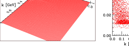
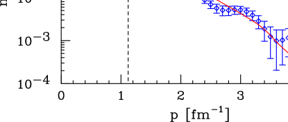
Figure 18: (color online). (Left) 3D plot of the spectral function for the ¹⁶O ground state based on the LDA approximation. (Middle) Scatter plot of the function shown in the left panel. (Right) The momentum distribution of nucleons in the ¹⁶O ground state. Solid line: LDA approximation. Dashed line: FG model with Fermi momentum $p_{F}$ = 221 MeV. Diamonds: Monte Carlo calculation based on the wave function of Ref. [152]. Figures taken from Ref. [145]. Copyright (2005) APS.

The large $p$ ($p\gg p_{F}$; the momentum $p$ is denoted by $k$ in Fig. 18 (left, middle)) and large $E$ ($E\gg e_{F}$) components of the spectral function are highly correlated. It is clear that a relativistic Fermi Gas model (RFG) assuming a uniform momentum distribution up to the Fermi momentum ($p_{F}$) in a uniform potential gives an inadequate description of the spectral function. It would be also informative to present the nucleon momentum distribution defined by

$$n(\bm{p}) = \int dE\,P(\bm{p},E)$$ (73)

$$= \langle 0|a^{\dagger}_{\bm{p}}\,a_{\bm{p}}|0\rangle\ ,$$ (74)

where $a^{\dagger}_{\bm{p}}$ ($a_{\bm{p}}$) denotes the creation (annihilation) operator of a nucleon with the momentum $\bm{p}$. The nucleon momentum distribution (labelled as LDA) shown in Fig. 18 (right) is obtained from the LDA-based spectral function shown in Fig. 18 (left, middle) by using Eq. (73). This is compared to the one calculated with a variational Monte Carlo calculation of Ref. [152]. Clearly, the LDA-based $n(\bm{p})$ is in good agreement with that based on the Monte Carlo calculation. We also show in Fig. 18 (right) $n(\bm{p})$ from the FG model corresponding to Fermi momentum $p_{F}$ = 221 MeV for a comparison. It is clear that the FG model gives a very different distribution.

After the NuInt12 Workshop [153], all the major neutrino experimental groups use the spectral function in calculating both QE and pion production cross sections, rather than a simple Fermi-Gas Model [149].

5.3 Final state interaction (FSI)

The cross section formula based on the IA scheme, Eq. (68), needs to be modified by taking account of the FSI. For this purpose, we employ the convolution scheme [154] where the IA cross section (Eq. (68)) is integrated with a folding function as

$$\frac{d\sigma^{\rm FSI}_{lA}}{d\omega d\Omega_{l^{\prime}}}=\int d\omega^{\prime}f_{\bm{q}}(\omega-\omega^{\prime})\frac{d\sigma^{\rm IA}_{lA}}{d\omega^{\prime}d\Omega_{l^{\prime}}}\ ,$$ (75)

where $\omega$ is the energy transfer from the lepton, and $f_{\bm{q}}(\omega)$ is the folding function through which the FSI effect is introduced. The folding function can be given by

$$f_{\bm{q}}(\omega)=\delta(\omega)\sqrt{T_{A}}+\big{(}1-\sqrt{T_{A}}\big{)}F_{\bm{q}}(\omega),$$ (76)

where $T_{A}$ denotes the nuclear transparency, and $F_{\bm{q}}(\omega)$ is a finite-width function. In the limit of full nuclear transparency, $T_{A}\to 1$, the IA cross section is recovered in Eq. (75).

Now let us connect the above convolution scheme for describing the FSI with an optical potential scattering. The FSI for the QE process can be described with an optical potential $U=U_{V}\ +\ iU_{W}$, originally proposed by Horikawa et al. [155] in the context of $(e,e^{\prime})$ processes. The real part of the potential, $U_{V}$, modifies the energy spectrum of the final-state nucleon, thereby shifting the cross section by $\omega\to\omega-U_{V}$. In the convolution scheme, this effect of $U_{V}$ can be accounted for by modifying the folding function as

$$f_{\bm{q}}(\omega-\omega^{\prime})\to f_{\bm{q}}(\omega-\omega^{\prime}-U_{V}).$$ (77)

Meanwhile, the imaginary part, $U_{W}$, re-distributes the transition strength of some of one-particle one-hole final states to more complex final states, leading to the quenching of the QE peak and the associated enhancement of its tails. In the convolution scheme, this effect of $U_{W}$ can be taken care of by using

$$F_{\bm{q}}(\omega)=\frac{1}{\pi}\frac{U_{W}}{U_{W}^{2}+\omega^{2}}\ ,$$ (78)

in Eq. (76). The remaining piece is the nuclear transparency $T_{A}$ in Eq. (76). In the calculation shown below, we use experimentally determined nuclear transparency of ¹²C reported in Ref. [156]. We also neglect the $|\bm{q}|$-dependence of $F_{\bm{q}}(\omega)$ in Eq. (76) and evaluate it at $|\bm{q}|$ = 1 GeV.

Having seen the relation between the optical potential $U$ and the folding function $f_{\bm{q}}(\omega)$, we now employ an optical potential that has been tested by data, and then plugged it into the folding function following the relation. With the folding function, the differential cross sections including the FSI effects are obtained from Eq. (75). We choose the proton-¹²C optical potential due to Cooper et al. [157] based on the Dirac phenomenology. In this framework, the optical potential consists of the scalar ($S$) and vector ($V$) parts appearing in the Dirac equation. Their dependence on the nucleon kinetic energy ($t_{\rm kin}$) and the radial coordinate $r$ has determined by fitting the data in the range of $29\leq t_{\rm kin}\leq 1040$ MeV. The scalar and vector potentials are related to the total energy of the proton $E^{\prime}_{\textrm{tot}}=E^{\prime}_{\textrm{tot}}(t_{\rm kin},r)$ by

$$E^{\prime}_{\textrm{tot}}(t_{\rm kin},r)=\sqrt{(m_{N}+S(t_{\rm kin},r))^{2}+p^{\prime 2}}+V(t_{\rm kin},r),$$ (79)

with $p^{\prime}$ being the nucleon’s momentum and related to $t_{\rm kin}$ by $t_{\rm kin}=p^{\prime\,2}/2m_{N}$. Here, as seen in Eqs. (77) and (78), the optical potential $U$ is treated as a $r$-independent quantity. Therefore, $U$ is defined as an average shift of the nucleon energy from the on-shell energy $E_{p^{\prime}}=\sqrt{m_{N}^{2}+p^{\prime 2}}$,

$$U=\int d^{3}r\rho(r)E^{\prime}_{\textrm{tot}}-E_{p^{\prime}}\ ,$$ (80)

which is calculated from the optical potential, $S$ and $V$, of the Dirac phenomenology. Regarding the density distribution of ¹²C, we extract it from the measured charge density [158] following the procedure in Ref. [159]. The real part of the optical potential ($U_{V}$) is presented in Fig. 19.

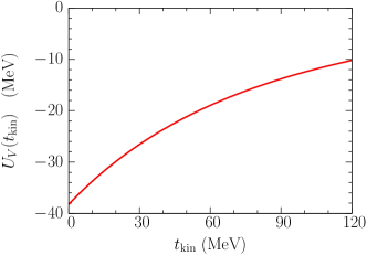
Figure 19: (color online). Real part of the proton-¹²C optical potential as a function of kinetic energy of the proton. The potential is related to the Dirac phenomenological fit of Cooper et al [157] through Eqs. (79) and (80). Figures taken from Ref. [147]. Copyright (2015) APS.

In the low $t_{kin}$ region, $U_{V}$ is large and negative as seen in the figure while the imaginary part ($U_{W}$) is small. Reference [147] and numerical results in the next subsection are mostly concerned with this energy region, and the above-described procedure was used in taking account of the FSI. On the other hand, in higher energy region ($>$ 200 MeV), $U_{V}$ becomes negligible and $U_{W}$ dominates. In this energy region, a different prescription based on a generalization of Glauber theory for including the FSI effects was taken in Ref. [145].

Since the nucleon kinematics is integrated over in Eq. (68), $t_{\rm kin}$ for $E^{\prime}_{\rm tot}$ and $T_{A}$ in using Eq. (75) is determined from the lepton kinematics

$$t_{\rm kin}=\frac{E_{l}^{2}(1-\cos\theta_{l^{\prime}})}{m_{N}+E_{l}(1-\cos\theta_{l^{\prime}})},$$ (81)

where $E_{l}$ and $\theta_{l^{\prime}}$ denote the incident lepton energy and the lepton scattering angle, respectively. This relation corresponds to scattering of a massless particle on a nucleon at rest.

5.4 Numerical results, comparison with electron scattering data

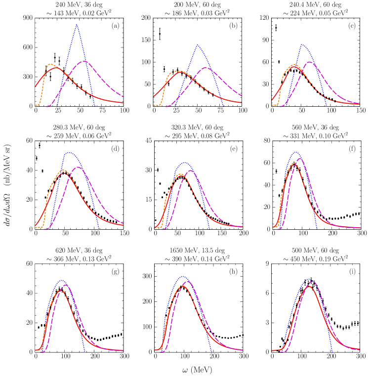
Figure 20: (color online). Differential cross sections, $d\sigma/d\omega d\Omega_{e^{\prime}}$, for electron-¹²C scattering; $\omega$ is the energy transfer to the nucleus. The results obtained with Pauli blocking accounted for in the local-density (solid lines) and step-function (short-dashed lines) approximations are compared to the experimental data from (a)-(g) Barreau et al. [160], (h) Baran et al. [161], and (i) Whitney et al. [162]. The IA (long-dashed lines) and RFG calculations (dotted lines) are also shown for reference. The panels are labeled according to beam energy, scattering angle, and values of $|\bm{q}|$ and $Q^{2}$ at the quasi-elastic peak. Figures taken from Ref. [147]. Copyright (2015) APS.

Comparison of the calculations with all existing inclusive ${}^{12}{\rm C}(e,e^{\prime})$ data in the energy region from $E_{e}$ = 0.2 to 2.0 GeV is shown in Fig. 20 [147]. These figures display double differential cross sections as a function of the energy transfer to the nucleus $\omega$ in the increasing order of the momentum transfer $|\bm{q}|$. The low $|\bm{q}|$ data show the contributions from discrete nuclear excitations including a giant dipole resonance and the elastic electron scattering in the small $\omega$ region, which are absent in the model. As $|\bm{q}|$ increases, the data start to cover the dip region between the QE peak and $\Delta(1232)$ peak in the large $\omega$ region.

The results obtained with the RFG model are shown by the dotted curves in Fig. 20. Parameters of the RFG model, Fermi momentum 221 MeV and separation energy $\epsilon=25$ MeV, were determined in Ref. [162] to fit the data shown in Fig. 20(i). Finding of the analysis is that even though the RFG model fits the data at this kinematics, the model predictions start to deviate from the data around the QE peak as $|\bm{q}|$ decreases. Within the RFG model, it is not possible to find a parameter set with which the model can fairly reproduce the $(e,e^{\prime})$ data in the broad kinematical region of interest for neutrino oscillation studies.

The results of the IA scheme without FSI are shown by the long-dashed curves while those including FSI and with the particle SF of Eq. (69) [Eq. (71)] are shown by the short-dashed [solid] curves in Fig. 20. Large contributions of FSI bring the IA results to fairly agreement with the data, especially around the QE peak from low to high $|\bm{q}|$ region. The effects of FSI are the redistribution of the strength from the peak to the tails due to the imaginary part of the optical potential and the shift of the cross section toward lower energy transfers due to the real part of the optical potential. The shift of the cross section is getting smaller for higher $|\bm{q}|$ (larger $t_{\rm kin}$), as expected from Fig. 19. The two prescriptions of the Pauli blocking, Eqs. (69) and (71), give very similar results near the QE peak. In the low $|\bm{q}|$ region, where Pauli blocking plays an important role, the LDA prescription of Eq. (71) may be slightly favored.

It is noticed that, at higher $|\bm{q}|$ and $\omega$ region, the results tend to underestimate the data beyond the QE peak, as in Figs. 20(d)-(i). In this dip region, two-particle–two-hole (2p2h) final states induced by two-nucleon correlations and two-nucleon currents as well as the other inelastic processes (e.g., pion production) would contribute to fill the gap [163, 164, 165]. Although initial (final) nucleon correlations have been taken into account in Ref. [147] through the nuclear spectral function (FSI), more elaborate treatment of FSI and inclusion of two-nucleon currents are needed. Analysis in this direction done with the spectral function formalism is reported in [166]. Also, recent works on 2p2h mechanisms and effects are reviewed in Ref. [12, 16].

6 Neutrino-nucleus reactions in the RES region

Recently, neutrino-nucleus scattering in the RES region, single pion productions in particular [43, 44, 167, 168], has been actively studied experimentally for better understanding the process and for developing a better model to be implemented in a generator. A microscopic description of this process is as follows. In the initial state, nucleons are bound in a nucleus under a certain energy and momentum distribution. The distribution is given by a Fermi gas model in the simplest treatment, and a more realistic distribution is given by a spectral function based on a shell model or an ab initio calculation [150]. Then an electroweak current interacts with one of the nucleons to produce a meson and the recoiled baryon. This process is described by elementary amplitudes such as those discussed in Sec. 3.3.4. The meson and baryon then propagate in the nucleus. In the course of the propagation, they can change their momenta and charges by interacting with the surrounding nucleons. The meson can even be absorbed by the nucleus, and a few nucleons are kicked out from the nucleus at the same time. These final state interactions (FSI) can be described, in principle, with a multiple scattering theory as those formulated, e.g., in Ref. [169]. More practically manageable formulation is the so-called $\Delta$-hole model [170, 171, 172, 173], more details of which will be discussed later in Sec. 6.2. However, these quantum mechanical calculations become a formidable task when dealing with a typical situation of the neutrino experiments where a few nucleons (and one or a few pions) are emitted from the nucleus. Because of the complexity of the problem, the most common treatment of the FSI has been to use a (semi)classical hadron transport model so far [20, 174, 175].

In the rest of this section, we discuss our own works on two particular cases that are relatively straightforward to deal with. One of them is neutrino-induced single pion productions off the deuteron. The old bubble chamber data are available for these processes [25, 73], and it has been well recognized that the data are valuable information from which the axial form factors associated with the $N$-$\Delta(1232)$ transition can be extracted. However, in the previous analyses, the nuclear effects, the FSI in particular, have not been taken into account in extracting the axial form factors. The deuteron is the simplest nucleus and thus the nuclear effects can be taken into account by explicitly dealing with interactions among all of mesons and baryons that appear in the process; no need to introduce a mean field nor phenomenological many-body effects. We will discuss our formalism and show significant nuclear effects in the following subsection. Another subject to be discussed in the subsequent subsection is coherent pion productions in the neutrino-nucleus scattering. In the coherent processes where the nucleus in the final state stays in its ground state, the FSI can be described with multiple iterations of an optical potential between the pion and the nucleus in the ground state. This is the situation where the $\Delta$-hole model is the most suitably applied. It is also timely to study the coherent process because this process has been studied experimentally recently [35, 45, 47, 176, 177, 209], and thus we can study how the $\Delta$-propagation is modified in nuclei by confronting calculations with the data.

6.1 Neutrino induced pion production reaction on deuteron

The neutrino-induced pion production reaction through $\Delta(1232)$ resonance plays a dominant role in the RES region as discussed in Sec. 3.3.4. This process is interesting from hadron physics point of view because we can study the axial vector $AN\Delta$ transition form factor, $C_{5}^{A}$ [Eq. (33)]. One can relate the $\pi N\Delta$ coupling constant with the $AN\Delta$ form factor assuming the PCAC, which however needs to be examined against cross section data. Information of the axial vector form factor can be obtained from a combined analysis of pion electroproductions and neutrino induced pion production reactions. Currently available data of the pion production reactions on the nucleon in the RES region are bubble chamber data from ANL [23, 73], BNL [25] and BEBC [26, 178], which are mainly data for neutrino-deuteron reactions. Consider the charged-current (CC) single pion production reactions on the deuteron: $\nu_{\mu}+d\rightarrow\mu^{-}+\pi^{+}+p+n$ and $\nu_{\mu}+d\rightarrow\mu^{-}+\pi^{0}+p+p$. The pion production cross sections for three channels

$$\nu_{\mu}+p \rightarrow \mu^{-}+\pi^{+}+p\ ,$$ (82)

$$\nu_{\mu}+n \rightarrow \mu^{-}+\pi^{+}+n\ ,$$ (83)

$$\nu_{\mu}+n \rightarrow \mu^{-}+\pi^{0}+p\ ,$$ (84)

have been extracted by assuming ’quasi-free’ pion production mechanism with the spectator nucleon. The first channel Eq. (82) is purely isospin $3/2$ reaction and is dominated by the $\Delta$ excitation. Especially the data for restricted $\pi N$ invariant mass region, $W<1.4$GeV, are useful to study the $\Delta$ resonance excitation. It has been recognized that there are some tension between the data of ANL and BNL [179, 180]. Recently, it has been demonstrated the ratios between the pion production process and the non-pion production quasi-elastic process of ANL and BNL are consistent with each other, which raises the questions on the normalization of the neutrino flux [87, 181, 182].

The cross section data for the three channels in Eqs. (82)-(84) will be modified by additional reaction mechanisms such as FSI of $\pi NN$ system, where a simple interpretation with a ’quasi-free’ reaction mechanism does not work. In fact, it is known the FSI among pion and nucleons are important in pion photoproductions on the deuteron [183, 184, 185, 186]. The FSI for the $\nu d$ reactions has been studied only recently by Wu et al. [74]. Here we briefly show the role of FSI following [74]. Within the first order correction of the multiple scattering theory [169], the transition amplitude of the neutrino-induced pion production can be written as a sum of impulse, nucleon-nucleon ($NN$) rescattering and pion-nucleon ($\pi N$) rescattering mechanisms,

$$T^{\mu}(d\rightarrow\pi NN) = <\pi NN|(1+(T_{NN}+T_{\pi N})G_{0})J^{\mu}|d>.$$ (85)

Here $J^{\mu}$ is a pion production weak current $N+J^{\mu}\rightarrow\pi+N$. The rescattering correction is taken into account by the second and the third terms of Eq. (85) using the nucleon-nucleon ($T_{NN}$), the pion-nucleon ($T_{\pi N}$) scattering t-matrix and the $\pi NN$ Green’s function ($G_{0}$) as shown in Fig. 21.

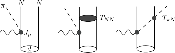
Figure 21: The impulse (left), $NN$ rescattering (middle) and $\pi N$ (right) rescattering mechanisms of Eq. (85).

Here we adopt a dynamical model developed in Refs. [65, 66, 83, 187] (called the SL model). to describe electroweak single pion production on the nucleon in the $\Delta$(1232) resonance region. The SL model has been well tested [83, 187] against the data of $\pi N$ scattering and electromagnetic pion production reactions on the nucleon in the $\Delta$(1232) resonance region. It also describes [65] well the cross sections of neutrino-induced single pion productions on the proton and neutron. We used the high precision Bonn nucleon-nucleon potential [188] to describe the deuteron and NN scattering state.

At first, we show that the current model describes well the available data of incoherent pion photo-production reactions on the deuteron. The results for the total cross sections of $\gamma+d\rightarrow\pi^{0}+n+p$ and $\gamma+d\to\pi^{-}+p+p$ as a function of the photon energy are shown in Fig. 22.

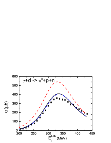
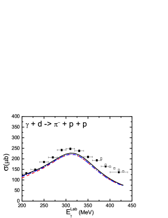
Figure 22: (Color online) The total cross sections of $\gamma+d\to\pi^{0}+n+p$ (Left) and $\gamma+d\to\pi^{-}+p+p$ (Right). The red dashed, blue dash-dotted, and black solid curves represent the impulse term , the impulse + ($NN$ FSI), and the impulse + ($NN$ + $\pi N$ FSI), respectively. This figure is taken from Ref. [74].

For the $\gamma+d\rightarrow\pi^{0}+n+p$ reaction, the cross section is greatly reduced when the $np$ FSI ($T_{NN}$ term) is added (dot-dashed curve) to the impulse term (dashed curve). The $\pi N$ FSI ($T_{\pi N}$ term) is also included in our full calculation (solid curve), which is a small effect. A similar comparison for the total cross sections of $\gamma+d\rightarrow\pi^{-}+p+p$ is shown. Here both the $pp$ and the $\pi N$ FSI are weak. Clearly, the $np$ re-scattering effects are very large for the $\pi^{0}$ production reaction, while effects of FSI is small for $\pi^{-}$ production reaction. Our full calculations are in reasonable agreement with the data in both $\pi^{0}$ and $\pi^{+}$ production reactions, while some improvements are still needed in the future. The result on the pion photoproductions shows that our calculational procedure is valid for predicting the $\nu+d\rightarrow\mu+\pi+N+N$ cross sections.

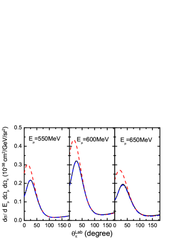
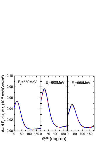
Figure 23: The differential cross sections $d\sigma/dE_{\mu^{-}}d\Omega_{\mu^{-}}d\Omega_{\pi}$ of $\nu_{\mu}+d\to\mu^{-}+\pi^{+}+p+n$ (left) and $\nu_{\mu}+d\to\mu^{-}+\pi^{0}+p+p$ (right) as function of $\theta_{\pi}^{LAB}$ in the laboratory system. See caption of Fig. 22. The figure is taken from Ref. [74].

Within the same calculational procedure as the pion photoproduction, we have studied the neutrino-induced pion productions on the deuteron: $\nu_{\mu}+d\rightarrow\mu^{-}+\pi^{+}+n+p$ and $\nu_{\mu}+d\rightarrow\mu^{-}+\pi^{0}+p+p$. The neutrino energy is chosen as $E_{\nu_{\mu}}=1$GeV with the angle between $\nu_{\mu}$ and $\mu^{-}$ set at $\theta_{\mu^{-}}=25^{\circ}$ and $E_{\mu}=550,600,650$ MeV. This kinematics is chosen to simulate the ’quasi-free’ $\Delta$ production process, where maximum values of the predicted cross sections are expected. The predicted pion angular distributions $d\sigma/dE_{\mu^{-}}d\Omega_{\mu^{-}}d\Omega_{\pi}$ are shown in Fig. 23. For $\nu_{\mu}+d\rightarrow\mu^{-}+\pi^{+}+n+p$ reaction, we have included contribution of pion production amplitudes from both proton and neutron. The $NN$ FSI is large at forward pion for $\nu_{\mu}+d\rightarrow\mu^{-}+\pi^{+}+n+p$ reaction, while it is small for the $\nu_{\mu}+d\rightarrow\mu^{-}+\pi^{0}+p+p$ reaction. The $\pi N$ FSI is small for both channels. The situation here is similar to what we have observed in the pion photoproductions that the FSI effects from the $np$ scattering are much larger than that from the $pp$ scattering. It may be understood by the orthogonality relation between bound state and scattering state of the ${}^{3}S_{1}$-${}^{3}D_{1}$ partial wave, which affects overlap integrals for low momentum transfer reactions.

In conclusion, the results strongly suggest that the spectator approximation used to extract the pion production cross sections on the nucleon from the data on the deuteron is not valid for the $\nu+d\rightarrow\mu^{-}+\pi^{+}+n+p$, but is a good approximation for $\nu+d\rightarrow\mu^{-}+\pi^{0}+p+p$. It will be important to extend this analysis to cover the whole kinematical region and examine the FSI effects on the total cross sections for the neutrino-induced pion production reactions on the deuteron. It will be also important to apply our approach to investigating the neutrino-deuteron reactions in the higher $W$ region where the higher mass nucleon resonances play important roles. Such an investigation can be performed with the coupled-channels model discussed in Sec. 3.3.4.

6.2 Coherent pion productions

Two different theoretical approaches have been taken to study the neutrino-induced coherent pion production. One of them is to use a model based on the PCAC relation [46, 189, 190, 191, 192, 193]. Because of the nuclear form factor, the coherent process is strongly suppressed when $Q^{2}$ departs from zero. In this situation, the amplitude is dominated by the divergence of the axial current that is related to the pion-nucleus elastic scattering amplitude through the PCAC relation. Another approach is to use a dynamical microscopic model [194, 195, 196, 197, 198, 199, 200, 201]. The model consists of ingredients such as elementary amplitudes, a nuclear form factor, and an optical potential for pion-nucleus elastic scattering. The nuclear effect on the $\Delta$ propagation also needs to be under control. Our model discussed below is classified into the latter approach. We do not go into details of each of the models, and refer the readers to a compact summary of the theoretical status given in Ref. [202].

Now we discuss our dynamical model for the coherent pion productions. It is based on the Sato-Lee (SL) model [65, 66] combined with a $\Delta$-hole model. The SL model is a prototype of the DCC model discussed in Sec. 3.3.4; it has only the $\pi N$ channel coupled to the $\Delta(1232)$ and is designed to work well in the $\Delta(1232)$ region. The $\Delta$-hole model accounts for the nuclear effects. Here we give a brief explanation of the $\Delta$-hole model for the elastic pion-nucleus scattering; for a full account, consult Refs. [170, 171, 172, 173].

In this formulation, the nuclear Fock space is divided into the nuclear ground state and a pion ($P_{0}$), one-particle one-hole and a pion ($P_{1}$), one-$\Delta$ one-hole ($D$), and all the other ($Q$); the symbols in the parentheses are the projection operators onto the corresponding nuclear Fock space, and thus $P_{0}+P_{1}+D+Q=1$. With the projection operator, we write a projected Hamiltonian as, for example, $H_{P_{0}D}=P_{0}HD$. Applying the projection operator method to Schrödinger equation in the full space, we can derive a Schrödinger equation defined in the subspace $P_{0}$ that describes the pion-nucleus elastic scattering. In the $\Delta$-hole model, we assume that the $D$-space is the doorway from the $P=P_{0}+P_{1}$ space to the $Q$ space, i.e., $H_{PQ}=H_{QP}=0$. Then we can write the pion-nucleus scattering amplitude that includes the $\Delta$ excitation as

$$T_{P_{0}P_{0}}(E)=H_{P_{0}D}G_{\Delta h}(E)H_{DP_{0}}\ ,$$ (86)

where the total energy in the center-of-mass frame is denoted by $E$. The quantity $G_{\Delta h}$ in Eq. (86) is $\Delta$-hole propagator that is more explicitly written by

$$G_{\Delta h}^{-1}=D(E-H_{\Delta})-W_{\rm el}-\Sigma_{\rm Pauli}-\Sigma_{\rm spr}\ .$$ (87)

We denoted the propagator of $\Delta$ in the vacuum with the invariant mass $W$ by $D(W)$, and write more explicitly as

$$D(W)=W-m_{\Delta}^{0}-\Sigma_{\Delta}(W)\ ,$$ (88)

where $m_{\Delta}^{0}$ and $\Sigma_{\Delta}$ are the bare mass and self energy of the $\Delta$-resonance, respectively. In Eq. (87), $H_{\Delta}$ is the Hamiltonian for the $\Delta$-particle in the nucleus. The effects associated with complicated configurations belonging to the $Q$-space such as multi-particle multi-hole states are very difficult to deal with microscopically, and thus the common practice is to squash them into the phenomenological $\Delta$ spreading potential [$\Sigma_{\rm spr}$ in Eq. (87)] that includes adjustable parameters to fit pion-nucleus scattering data. The model takes account of couplings to the $P_{1}$-space through the $\Delta$ self energy $\Sigma_{\Delta}(W)$ included in $D(E-H_{\Delta})$ [see Eq. (88)] with a correction $\Sigma_{\rm Pauli}$ associated with the Pauli blocking. Couplings to the $P_{0}$-space denoted by $W_{\rm el}$ in $G_{\Delta h}$ describe the elastic rescattering. A calculation of the pion-nucleus elastic amplitude in Eq. (86) needs a diagonalization of $G_{\Delta h}$ which is numerically rather involved. Here, we employ a simplified treatment of $G_{\Delta h}$ proposed by Karaoglu and Moniz [203], based on the local density approximation. A resonant amplitude for coherent pion production induced by an electroweak current can be obtained from Eq. (86) by replacing $H_{DP_{0}}$ with $H_{DP_{0}^{\prime}}$ where $P_{0}^{\prime}$ is the space spanned by the external electroweak current and the nucleus in the ground state. We emphasize here that our framework treats the medium effect on the $\Delta$ propagation in the pion-nucleus scattering and also in electroweak pion productions on the same footing. Because of this consistency, we can make a parameter-free prediction for electroweak coherent pion production cross sections, once we determine parameters associated with the medium effects, i.e., those included in $\Sigma_{\rm spr}$, by fitting the pion-nucleus scattering data. Our numerical analysis will also be done in this ordering. We refer the readers to Ref. [200] to find more explicit and detailed formulas for the quantities in Eqs. (86)-(88) and for coherent pion production amplitudes that are actually implemented in numerical calculations.

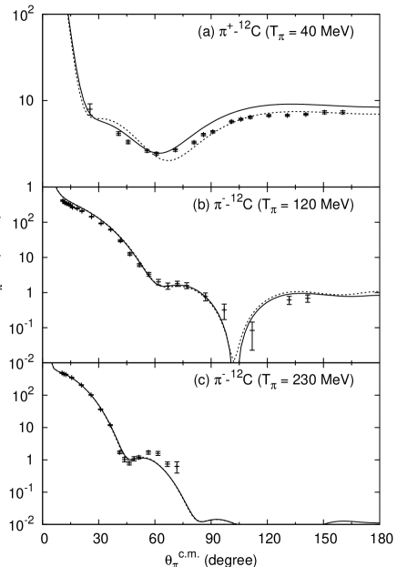
Figure 24: $\pi$-¹²C elastic differential cross sections. The full calculations are shown by the solid curves while the results obtained without the phenomenological $\rho^{2}$-term are shown by the dashed curves. The data are from Ref. [204] for (a) and Ref. [205] for (b) and (c). Figures taken from Ref. [200]. Copyright (2010) APS.

From now we present our numerical results. The first thing to do is to analyze pion-nucleus scattering data. The pion-nucleus optical potential derived from the SL combined with the $\Delta$-hole model is the main driving force for this process. We have two complex adjustable parameters in $\Sigma_{\rm spr}$. In addition, we also consider a phenomenological term that are proportional to the square of the nuclear density; this term simulates the pion absorption by two nucleons through non-$\Delta$ mechanism. Then we have additional two complex adjustable parameters. After all, we fit the data for both elastic and total cross sections in and around the $\Delta$ region by adjusting totally eight free parameters. The quality of the fit can be seen in Fig. 24 where our calculations for the $\pi$-¹²C elastic differential cross sections are compared with the data. The agreement between our calculations and the data are reasonably good. We note that a good agreement is also obtained between our calculation and pion-nucleus total cross section data.

Figure 25: Differential cross sections for $\gamma+{}^{12}{\rm C}_{g.s.}\to\pi^{0}+{}^{12}{\rm C}_{g.s.}$. The incident photon energy is $E_{\gamma}^{\rm LAB}$=173 MeV for (a) and $E_{\gamma}^{\rm CM}$=290 MeV for (b). The solid curves are from the full calculations while the dashed curves are obtained without the FSI and without the medium effects on the $\Delta$-propagation. The dotted curves are obtained with the medium effects on the $\Delta$ included. By considering only the $\Delta$ mechanism in the pion production operator, we obtained the dash-dotted curves. The data are from Ref. [206] for (a) and from Ref. [207] for (b). Figures taken from Ref. [200]. Copyright (2010) APS.

With the parameters fixed in the above analysis, we can then make a parameter-free prediction for coherent pion productions. First, we calculate photon-induced coherent pion production for which data with a good quality are available. The photoproduction is a good testing ground to examine the reliability of our model. In Fig. 25, we show a comparison of our numerical results for the differential cross sections for $\gamma+{}^{12}{\rm C}_{g.s.}\to\pi^{0}+{}^{12}{\rm C}_{g.s.}$ with data [206, 207]. Different curves in each panel include different dynamical contents. The dashed curves include neither FSI nor the medium effects on $\Delta$-propagation. By including the medium effects on the $\Delta$, the dotted curves are obtained. Finally our full calculation gives the solid curves. Clearly, the medium effects are large and important in achieving a good agreement with the data. Particularly in the $\Delta$ region [Fig. 25 (b)], the medium effects work to absorb pions, leading to the drastic reduction of the cross sections. The obtained good agreement seen in Fig. 25 indicates the soundness of our approach, and encourages us to apply the same approach to the neutrino-induced coherent pion productions. An interesting feature seen in Fig. 25 is that the non-resonant contribution (the difference between the solid and dash-dotted curves) is significant even in the energy near the $\Delta(1232)$ peak [Fig. 25(b)]. This is partly due to the fact that the resonant contribution is significantly reduced by the pion absorptions.

Figure 26: The total cross sections as a function of $E_{\nu}$ for $\nu_{\mu}+{}^{12}{\rm C}_{g.s.}\to\mu^{-}+\pi^{+}+{}^{12}{\rm C}_{g.s.}$ (solid curve), $\nu+{}^{12}{\rm C}_{g.s.}\to\nu+\pi^{0}+{}^{12}{\rm C}_{g.s.}$ (dashed curve), $\bar{\nu}_{\mu}+{}^{12}{\rm C}_{g.s.}\to\mu^{+}+\pi^{-}+{}^{12}{\rm C}_{g.s.}$ (dotted curve) and $\bar{\nu}+{}^{12}{\rm C}_{g.s.}\to\bar{{\nu}}+\pi^{0}+{}^{12}{\rm C}_{g.s.}$ (dash-dotted curve). Figure taken from Ref. [200]. Copyright (2010) APS.

We now move on to neutrino-induced coherent pion productions on ¹²C target. We consider the CC processes, $\nu_{\mu}(\bar{\nu}_{\mu})+{}^{12}{\rm C}_{g.s.}\to\mu^{-}(\mu^{+})+\pi^{+}(\pi^{-})+{}^{12}{\rm C}_{g.s.}$, and the NC processes, $\nu(\bar{\nu})+{}^{12}{\rm C}_{g.s.}\to\nu(\bar{\nu})+\pi^{0}+{}^{12}{\rm C}_{g.s.}$. The total cross sections for these processes are shown in Fig. 26 as functions of the incident neutrino (anti-neutrino) energy in the laboratory system. As expected from the isospin factor, we find $\sigma_{\rm CC}/\sigma_{\rm NC}\sim 2$ for higher $E_{\nu}$. On the other hand, $\sigma_{\rm NC}$ becomes larger than $\sigma_{\rm CC}$ at low $E_{\nu}$ because the massless lepton in the final state gives the NC processes a larger phase space. The difference between the neutrino and antineutrino processes is from the interference between the vector and axial currents. Because the axial current dominates in the coherent processes, this interference gives a rather small contribution.

We compare our result with available data. In order to do so, we average the cross sections by convoluting with the neutrino flux that was used in the experiment. We use the neutrino fluxes of $E_{\nu}\leq$ 2 GeV, and neglect the fluxes beyond that limit. To compare with a K2K result for the CC process [35], we use the flux reported in Ref. [208] and obtain $\sigma_{\rm ave}^{\rm CC}=6.3\times 10^{-40}{\rm cm}^{2}$. Our result is consistent with the upper limit from the K2K experiment; $\sigma_{\rm K2K}<7.7\times 10^{-40}{\rm cm}^{2}$. This upper limit was obtained with some kinematical cuts which we also applied to our calculation. A similar upper limit was also reported from a SciBooNE experiment [45]. For other theoretical calculations compared with the K2K result, see Table 1. Nonzero CC coherent pion productions at low energies ($E_{\nu}\ \raise 1.29167pt\hbox{$<$\kern-7.5pt\lower 4.30554pt\hbox{$\sim$}}\$ 1 GeV) have been recently reported by the T2K Collaboration [209]. They performed two analyses in each of which a different coherent pion production model was used: the models of Rein-Sehgal [46] and Alvarez-Ruso et al. [196, 197]. The data were collected within a restricted phase space, defined by $p_{\mu}>$ 0.18 GeV, $0.18<p_{\pi}<1.6$ GeV, and $\theta_{\mu(\pi)}<70^{\circ}$, where the detector has a good acceptance; $p_{\mu(\pi)}$ is the momentum of $\mu$ ($\pi$) and $\theta_{\mu(\pi)}$ is the angle between the $\mu$ ($\pi$) momentum and the incident neutrino direction. The flux-averaged cross section to the restricted phase space was found to be $3.2\pm 0.8({\rm stat})^{+1.3}_{-1.2}({\rm sys})$ ($2.9\pm 0.7^{+1.1}_{-1.1}$) $\times 10^{-40}\,{\rm cm}^{2}$ when the model of Rein-Sehgal [46] (Alvarez-Ruso et al. [196, 197]) was used. Then, the flux-averaged total cross section was estimated using the model predictions for the unmeasured phase space. $3.9\pm 1.0^{+1.5}_{-1.4}$ ($3.3\pm 0.8^{+1.3}_{-1.2}$) $\times 10^{-40}\,{\rm cm}^{2}$ was obtained for the model of Rein-Sehgal [46] (Alvarez-Ruso et al. [196, 197]). We update our calculation of Ref. [200] to compare with this new data covering the full phase space. For this purpose, cross sections are convoluted with the neutrino flux for the T2K experiment [210] that peaks at $E_{\nu}\sim 0.6$ GeV. Our result, $3.1\times 10^{-40}\,{\rm cm}^{2}$, is in a good agreement with the T2K result.

Channel (EXP.)	CC$\pi^{+}$(K2K)	CC$\pi^{+}$(T2K)	NC$\pi^{0}$(MiniBooNE)
Data	$<7.7$ [35]	$3.3\pm 0.8^{+1.3}_{-1.2}$ [209]	$7.7\pm 1.6\pm 3.6$ [211]
		$3.9\pm 1.0^{+1.5}_{-1.4}$ [209]
Alvarez-Ruso et al. [196, 197]	8.3 (4.4)	5.3 [209]	3.9 (2.0)
Berger et al. [192]	0.62$\times$12	–	–
Nakamura et al. [200]	6.3	3.1 [This work]	2.8
Hernández et al. [201]	$6.1\pm 1.3$	–	$2.6\pm 0.5$

Table 1: CC and NC coherent pion production cross sections from several theoretical calculations in comparison with data. The unit is $10^{-40}{\rm cm}^{2}$. In the second, third, and fourth columns, theoretical cross sections have been convoluted with the neutrino fluxes used in K2K [208], T2K [210], and MiniBooNE [212] experiments, respectively. The two results of the T2K [209] are from different analyses in which different coherent pion production models were used. See the text for more explanation on the T2K data. The numbers in the parentheses from Alvarez-Ruso et al. are obtained with different form factors.

Regarding the NC process, the MiniBooNE Collaboration reported the flux-averaged cross section, $\sigma_{\rm MiniBooNE}=7.7\pm 1.6\pm 3.6\times 10^{-40}{\rm cm}^{2}$ [211]. Using the same flux as given in Ref. [212], we obtain $\sigma_{\rm NC}=2.8\times 10^{-40}{\rm cm}^{2}$ which is barely consistent with the MiniBooNE result. A similar tendency is also found in comparisons of other theoretical calculations tabulated in Table 1 with the data. Furthermore, the SciBooNE Collaboration published the ratio between CC and NC coherent pion production cross sections [177]: $\sigma_{\rm CC}/\sigma_{\rm NC}=0.14^{+0.30}_{-0.28}$. On the other hand, our as well as all the other theoretical calculations after 2005 gave rather different results, $\sigma_{\rm CC}/\sigma_{\rm NC}=1.5\sim 2$, which is expected from the isospin factor. Several authors [198, 200, 201] have suspected that this puzzling situation could arise from the fact that the RS model [46, 189] was used in the analyses of the NC data. They showed that $\eta$-distribution $(\eta\equiv E_{\pi}(1-\cos\theta_{\pi}))$ of the RS model is rather different from those of their microscopic models. In the NC data analyses, the $\eta$-distribution has been proven useful in separating $\pi^{0}$ events into each production mechanism. Thus one may suspect this analyses could have overestimated the NC cross sections. It would be interesting to re-analyze the data with a more realistic coherent pion production model.

Figure 27: The pion momentum distribution in $\nu_{\mu}+\!{}^{12}{\rm C}_{g.s.}\to\mu^{-}\!+\!\pi^{+}\!+\!{}^{12}{\rm C}_{g.s.}$ at $E_{\nu}$ = 1 GeV; $p_{\pi}$ is the pion momentum in the laboratory frame. The solid, dashed, dotted and dash-dotted curves include the same dynamical features as those in Fig. 25. Figure taken from Ref. [200]. Copyright (2010) APS.

Finally, we discuss the pion momentum distribution in the neutrino-induced coherent pion production to see an impact of the nuclear effects on the observables. In Fig. 27, we show our result for $\nu_{\mu}+{}^{12}{\rm C}_{g.s.}\to\mu^{-}+\pi^{+}+{}^{12}{\rm C}_{g.s.}$ at $E_{\nu}$=1 GeV. As we have seen in the photon-induced coherent pion production (Fig. 25), we again find large medium effects here. The pion is significantly absorbed near the $\Delta$ peak, and the peak position is shifted by the FSI. It is also shown in the figure that the non-resonant amplitudes contributes to enhance the cross section by 18% in this case. We note that the rescattering effect significantly enhances the non-resonant contribution. This is in contrast with the other microscopic calculations for the neutrino-induced coherent pion productions that found little role of (tree-level) non-resonant mechanisms.

7 Neutrino-nucleus reactions in the DIS region

7.1 Nuclear modifications of structure functions

The structure function $F_{2}$ for the nucleon has been measured in a wide kinematical region from small $x$ ($\sim 10^{-4}$) to large $x$ ($\sim 0.8$) and from small $Q^{2}$ ($\sim 1$ GeV²) to large $Q^{2}$ ($\sim 10^{4}$ GeV²). In 1970’s when the DIS experiments started, people expected that the nuclear structure functions were simple additions of proton and neutron contributions. Therefore, it was rather surprising that a nuclear modification of $F_{2}$ was found by the European Muon Collaboration (EMC) in 1983 [213], although the Fermi-motion part in the large $x$ region was theoretically discussed before this experiment.

Figure 28: Measurements for the nuclear modification ratio $F_{2}^{C}/F_{2}^{D}$, where $C$ and $D$ indicate carbon and deuteron, respectively.

Since nuclear binding energies are negligible in comparison with DIS energies of more than multi GeV, noticeable nuclear effects were not expected except for the large-$x$ region before the EMC’s discovery. The current situation of nuclear modifications are shown in Fig. 28 for the carbon nucleus by the ratio $F_{2}^{C}/F_{2}^{D}$. At small $x$ ($<0.05$), the ratio is smaller than one and it is caused by nuclear shadowing, whereas the enhancement at $x\sim 0.1$ is called anti-shadowing. The modifications are also negative in the medium $x$ ($0.3<x<0.7$) due to nuclear binding and possibly nucleon’s internal modification, and the ratio increases at large $x$ ($>0.8$) due to the Fermi motion of the nucleon. The nuclear modification mechanisms are explained in Ref. [214].

The range of the scaling variable $x$ is $0<x<A$ for a nucleus of the mass number $A$ while $0<x<1$ for the nucleon. If the variable is defined by $x_{A}=Q^{2}/(2p_{A}\cdot q)=Q^{2}/(2\bar{M}_{A}\nu)$, the range is given by $0<x_{A}<1$ in the same way as the nucleon. Here, $\bar{M}_{A}$ and $p_{A}$ are nuclear mass and momentum, respectively. The mass difference from the nucleon gives rise to the relation, $x=(\bar{M}_{A}/m_{N})x_{A}\simeq Ax_{A}$, so that we have $0<x<A$. Since there is no DIS data in the region $x>1$, the extremely large-$x$ region is neglected in our analysis of the NPDFs.

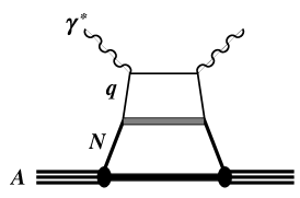
Figure 29: Convolution description for nuclear structure functions.

For describing nuclear structure functions at medium and large $x$, we may use a simple convolution description as shown in Fig. 29. The hadron tensor for a nucleus $W_{\mu\nu}^{A}$ is expressed by the one for the nucleon $W_{\mu\nu}^{N}$ convoluted with the spectral function $S(p_{N})$ for a nucleon in the nucleus [214, 215]:

$$W_{\mu\nu}^{A}(p_{A},q)=\int d^{4}p_{N}\,S(p_{N})\,W_{\mu\nu}^{N}(p_{N},q).\vspace{-0.10cm}$$ (89)

Namely, the quark distributions in the nucleon are modified by the effect of the nucleon energy-momentum distribution in the nucleus $S(p_{N})$, and they are estimated by the convolution integral. Then, the projection operator $\hat{P}_{2}^{\,\mu\nu}=-\bar{M}_{A}\,p_{A}\cdot q/(2\,\tilde{p}_{A}^{\,2})\left(g^{\mu\nu}-3\,\tilde{p}_{A}^{\,\mu}\,\tilde{p}_{A}^{\,\nu}/\tilde{p}_{A}^{\,2}\right)$, $\tilde{p}_{A}^{\,\mu}=p_{A}^{\,\mu}-(p_{A}\cdot q)q^{\,\mu}/q^{2}$ is applied to extract the $F_{2}$ structure function from $W_{\mu\nu}^{A}$:

$$F_{2}^{A}(x,Q^{2}) =\int_{x}^{A}dy\,f(y)\,F_{2}^{N}(x/y,Q^{2}),$$

$$f(y) =\int d^{4}p_{N}\,S(p_{N})\,y\,\delta\left(y-\frac{p_{N}\cdot q}{m_{N}\nu}\right),\ \ y=\frac{\bar{M}_{A}\,p_{N}\cdot q}{m_{N}\,p_{A}\cdot q}\simeq\frac{A\,p_{N}^{+}}{p_{A}^{+}},$$ (90)

where the lightcone momentum is defined by $p^{+}=(p^{0}+p^{3})/\sqrt{2}$. The spectral functions $S(p_{N})$ have been investigated in electron scattering studies. Using them in the convolution integral, we can calculate the effects of binding, Fermi motion, and short-range correlations in $F_{2}^{A}/F_{2}^{D}$. However, they may not be enough to explain the whole nuclear modifications observed experimentally, and modifications of the internal structure of the nucleon in $F_{2}^{N}$ could be needed [216].

On the other hand, the small-$x$ part is modified by a different mechanism of nuclear shadowing. In charged-lepton scattering, virtual photon ($\gamma^{*}$) transforms into a vector meson or corresponding $q\bar{q}$ state because they have the same quantum numbers. Using the photon momentum $q=(\nu,{\rm{}}0,{\rm{}}0,{\rm{}}-\sqrt{\nu^{\rm{2}}+Q^{2}})$, we have the propagation length of the vector meson as $\lambda=1/|E_{V}-E_{\gamma}|\simeq 2\nu/(M_{V}^{2}+Q^{2})=0.2\ {\rm{fm}}/x>2\ {\rm{fm\ at\ }}x<0.1$. It is larger than the average nucleon separation in a nucleus (2.2 fm). The $F_{2}$ structure function is expressed by the $\gamma^{*}A$ cross section as $F_{2}^{A}(x,Q^{2})\simeq Q^{2}\sigma_{\gamma^{*}A}/(4\pi^{2}\alpha)$ at small $x$, where $\alpha$ is the fine structure constant. We consider the picture that the virtual photon interacts as the vector meson or $q\bar{q}$ state ($h$) with a nucleus, and then structure function $F_{2}$ is expressed by the hadron-nucleus cross section $\sigma_{hA}$ and spectral function of the hadronic state $\Pi(s)$ as

$$\!\!\!F_{2}^{A}(x,Q^{2}) =\frac{Q^{2}}{\pi}\int_{4m_{\pi}^{2}}^{\infty}dM^{2}\frac{M^{2}\,\Pi(M^{2})}{\left(M^{2}+Q^{2}\right)^{2}}\;\sigma_{hA}(M^{2}),\ \ \Pi(s) =\frac{1}{12\pi^{2}}\frac{\sigma_{e^{+}e^{-}\rightarrow{\rm hadrons}}(s)}{\sigma_{e^{+}e^{-}\rightarrow\mu^{+}\mu^{-}}(s)},$$ (91)

where $\Pi(s)$ contains vector-meson and $q\bar{q}$-continuum contributions. Because the hadron propagation length is longer than the average nucleon separation, the hadron $h$ interacts with a nucleon not only once but also multiple times. This process is described by multiple scattering theory, and it gives rise to the nuclear shadowing. In the weak interactions, the axial vector current contributes to the cross section in addition to the vector one, so that the axial-vector mesons (or corresponding $q\bar{q}$ states) contribute to the shadowing. Here, we do not explain more about the nuclear modifications by the convolution picture and the shadowing phenomena so one may read Ref. [214] for the details.

7.2 Parton distribution functions in nuclei

As discussed in the previous section, we know the $x$ dependence of nuclear modifications from experimental measurements for various nuclei, and major theoretical ideas have been proposed to explain the nuclear modifications observed experimentally. If the order of nuclear effects is merely needed, or if only the gross properties of nuclear structure functions are studied, such theoretical models are good enough to predict the nuclear structure functions for estimating neutrino-nucleus cross sections. However, it is not the case in the current neutrino experiments. Accurate theoretical cross sections are needed for neutrino oscillation experiments where uncertainties associated with the current understanding of the neutrino-nucleus interactions are the dominant sources of systematic errors. The theoretical models are valuable for us to understand the physics behind the nuclear modifications; however, they may not provide predictions accurate enough for high-energy neutrino reactions. Therefore, it is usual to use a global analysis result for the NPDFs in the same way that the global-analysis PDFs are used for Large Hadron Collider (LHC) analysis for finding new physics beyond the standard model.

One could determine the NPDFs by parametrizing them in the same way as the nucleonic PDF analysis. However, it is practically more useful to express the NPDFs in terms of the nucleonic PDFs by assigning nuclear modification factors $w_{i}(x,A,Z)$ at the initial $Q^{2}$ scale ($\equiv Q_{0}^{2}$) as [217]

$$u_{v}^{A}(x,Q_{0}^{2}) =w_{u_{v}}(x,A,Z)\,\frac{1}{A}\left[Z\,u_{v}(x,Q_{0}^{2})+Nd_{v}(x,Q_{0}^{2})\right],$$

$$d_{v}^{A}(x,Q_{0}^{2}) =w_{d_{v}}(x,A,Z)\,\frac{1}{A}\left[Z\,d_{v}(x,Q_{0}^{2})+Nu_{v}(x,Q_{0}^{2})\right],$$

$$\bar{u}^{\,A}(x,Q_{0}^{2}) =w_{\bar{u}}(x,A,Z)\,\frac{1}{A}\left[Z\,\bar{u}(x,Q_{0}^{2})+N\bar{d}(x,Q_{0}^{2})\right],$$

$$\bar{d}^{\,A}(x,Q_{0}^{2}) =w_{\bar{d}}(x,A,Z)\,\frac{1}{A}\left[Z\,\bar{d}(x,Q_{0}^{2})+N\bar{u}(x,Q_{0}^{2})\right],$$

$$\bar{s}^{\,A}(x,Q_{0}^{2}) =w_{\bar{s}}(x,A,Z)\,\bar{s}(x,Q_{0}^{2}),$$

$$g^{\,A}(x,Q_{0}^{2}) =w_{g}(x,A,Z)\,g(x,Q_{0}^{2}),$$ (92)

because the nucleonic PDFs have been determined accurately in a wide kinematical region of $x$ and $Q^{2}$ and nuclear modifications are of the order of 10-20%. Furthermore, nuclear data are often shown in ratio forms such as $F_{2}^{A}/F_{2}^{D}$, so that the modifications could be obtained more easily rather than the absolute distributions. Here, $w_{i}$ is the nuclear modification factor to be determined by a global analysis, $i$ is a parton species, and $A$, $Z$, and $N$ are mass, atomic, and neutron numbers. The functional form of Eq. (92) cannot describe the NPDFs at $x>1$; however, it is not an issue at this stage because there is no DIS data in such an extremely large-$x$ region. The scale $Q_{0}^{2}$ is taken as $Q_{0}^{2}=1$ GeV² in our analysis, so that the charm-quark modification factor $w_{c}(x,A,Z)$ does not exist. Although we found an effect on the NuTeV anomaly about $\sin^{2}\theta_{W}$ from the nuclear modification difference between $u_{v}$ and $d_{v}$ in Ref. [218], it is impossible to determine it from experimental measurements at this stage [219]. Therefore, the parameters in $w_{u_{v}}$ and $w_{d_{v}}$ are assumed to be the same except for one-type parameters (such as $a_{u_{v}}$ and $a_{d_{v}}$ in Eq. (93)), which are fixed independently by the baryon-number and charge conservations, in our current parametrization. Furthermore, the antiquark modifications are assumed equal $w_{\bar{u}}=w_{\bar{d}}=w_{\bar{s}}\equiv w_{\bar{q}}$ although they could be different [220, 221].

We try to determine the nuclear modification parts $w_{i}(x,A,Z)$ by a global analysis of world data on high-energy nuclear reactions. The functions are parametrized in the form

$$w_{i}(x,A,Z)=1+\left({1-\frac{1}{{A^{\alpha}}}}\right)\frac{{a_{i}+b_{i}x+c_{i}x^{2}+d_{i}x^{3}}}{{(1-x)^{\beta}}},$$ (93)

with the parameters $\alpha$, $\beta$, $a_{i}$, $b_{i}$, $c_{i}$, and $d_{i}$. At this stage, there is no solid data to separate flavor-dependent nuclear effects, and thus we take $i=u_{v}$, $d_{v}$, $\bar{q}$, and $g$ as the parton species. The cubic functional form is employed in the numerator of the second term of Eq. (93) in order to have similar $x$-dependent variations as in Fig. 28. The initial scale $Q_{0}^{2}$ is arbitrary as long as it is taken in the region where perturbative QCD can be applied. In order to avoid higher-twist effects, it is desirable to take it more than a few GeV². However, the electron-ion collider like HERA does not exist for nuclei at this stage, which limits the kinematical region of measured structure functions. This fact inevitably leads to small $Q^{2}$ values at small $x$ in the structure-function measurements. In order to include valuable shadowing information at small $x$, we may take $Q_{0}^{2}=1\ {\rm GeV}^{2}$. However, the small $Q^{2}$ region could contain the higher-twists effects, which are neglected so far in our analysis. There are three obvious constraints for the NPDFs from the conservations of baryon number, charge, and momentum:

$$\begin{array}[]{ll}{\text{Baryon number:}}&A\int dx\left[\frac{1}{3}u_{v}^{A}(x)+\frac{1}{3}d_{v}^{A}(x)\right]=A,\\[6.0pt] {\text{Charge:}}&A\int dx\left[\frac{2}{3}u_{v}^{A}(x)-\frac{1}{3}d_{v}^{A}(x)\right]=Z,\\[6.0pt] {\text{Momentum:}}&A\sum\limits_{i=q,\bar{q},g}\int dx\,xf_{i}^{A}(x)=A,\end{array}\vspace{-0.10cm}$$ (94)

where $f_{i}^{A}(x)$ indicates the PDFs $f_{u}^{A}(x)=u^{A}(x)$, $f_{d}^{A}(x)=d^{A}(x)$, and so on. Therefore, the parameters in Eq. (93) are determined in a global $\chi^{2}$ analysis under the three constraints of Eq. (94).

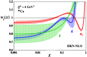
Figure 30: HKN nuclear modifications at $Q^{2}=4$ GeV².

The nuclear modification functions $w_{i}(x,A,Z)$, more specifically the parameters introduced in Eq. (93), are determined by a global analysis of charged-lepton DIS measurements on the ratios $F_{2}^{A}/F_{2}^{D}$ and $F_{2}^{A}/F_{2}^{A^{\prime}}$ and Drell-Yan ratios $\sigma_{DY}^{pA}/\sigma_{DY}^{pD}$ [217]. The NPDFs of Eq. (92) are evolved to the experimental $Q^{2}$ points by the standard DGLAP (Dokshitzer-Gribov-Lipatov-Altarelli-Parisi) evolution equations [222] for calculating the $\chi^{2}$ values. The functions $w_{i}$ are shown in Fig. 30 with the uncertainty bands estimated by using the Hessian matrix obtained in the $\chi^{2}$ fit. The valence-quark distributions are well determined for $x>0.3$ because the valence-quark distributions dominate the structure function $F_{2}^{A}$ at medium and large $x$ ($>0.3$) and there are many experimental data, as typically seen in Fig. 28, to constrain the valence-quark modification $w_{u_{v}}$ and $w_{d_{v}}$ ($=w_{u_{v}}$ for an isoscalar nucleus ⁴⁰Ca) at $x>0.3$. The antiquark distributions dominates $F_{2}$ at small $x$, so that the antiquark modification $w_{\bar{q}}$ is also determined well in the shadowing region at $x<0.05$ by the $F_{2}$-ratio data. The function $w_{\bar{q}}$ is also fixed by the Drell-Yan data, which indicated almost no nuclear modification in the region $0.05<x<0.2$. If there is no nuclear modification for the antiquark distributions at $0.1<x<0.2$, the anti-shadowing data, typically seen as the positive modification at $x\sim 0.1$ in Fig. 28, should be interpreted as the positive nuclear effects in the valence-quark distributions. This is the reason why the function $w_{u_{v}}$ is also determined well at $0.1<x<0.2$. Because of the baryon-number and charge conservations in Eq. (94), the valence-quark modifications at small $x$ are constrained by the same functions determined for $x>0.1$. Therefore, the valence-quark functions have small uncertainties in the whole-$x$ region. The antiquark distributions at $x>0.2$ are not determined by the current measurements and have large errors as shown in Fig. 30. The gluon distribution in the nucleon is determined mainly by the scaling violation of $F_{2}$. However, the scaling violation is not obvious experimentally in the ratios $F_{2}^{A}/F_{2}^{A^{\prime}}$, which makes it difficult to pin down the gluon nuclear modification $w_{g}$ as shown by the large uncertainty band in Fig. 30. Including LHC data, we hope to find more accurate gluon distributions in nuclei.

In our studies, the distributions defined by Eq. (92) are called NPDFs by considering a nucleus as a whole system in the same way as the nucleonic PDF. However, the distributions $f_{i}^{p/A}$ are sometimes called NPDFs for the parton type $i$ by other groups [223] with the definition $f_{i}^{A}(x,Q_{0}^{2})=[\,Z\,f_{i}^{p/A}(x,Q_{0}^{2})+Nf_{i}^{n/A}(x,Q_{0}^{2})\,]\,/A$ by considering proton and neutron contributions in a nuclear medium, and they should not be confused with our NPDFs $f_{i}^{A}(x,Q_{0}^{2})$. If both definitions are not confused, the choice does not matter. In comparing the nuclear modifications of various groups, we should be careful about this difference in the definition.

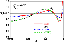
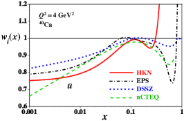
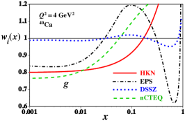
Figure 31: Comparison of various nuclear PDFs at $Q^{2}=4$ GeV² for ⁴⁰Ca.

Determined HKN NPDFs are compared with other analysis results [223] in Fig. 31. All the distributions are similar except for the gluon modifications at small $x$ and antiquark/gluon modifications at medium $x$ because they are not well constrained by experimental measurements. However, the LHC experiments are in progress and they are generally sensitive to small-$x$ NPDFs, so that the gluon shadowing should be determined more reliably by including LHC measurements. In fact, a large gluon shadowing is suggested by studying productions of vector mesons at LHC [224]. On the other hand, in comparison with the LHC data on charged-hadron, dijets, and direct-photon productions in p+Pb, the current NPDFs seem to be consistent [225]. There is a possibility that nuclear modifications are flavor dependent as studied in Refs. [219, 220], and such effects may be found in neutrino DIS data. In fact, flavor-dependent nuclear modifications were recently investigated by the nCTEQ collaboration [223]. However, there is no clear data at this stage to indicate the flavor dependence for valence-quark and antiquark modifications. There is also Drell-Yan experiment in progress at Fermilab to probe the flavor dependence and nuclear modifications in antiquark distributions by the E906-SeaQuest collaboration [226]. The flavor dependence could be investigated by a future JLab experiment [227], and the full analysis of nuclear EMC ratio $F_{2}^{A}/F_{2}^{D}$ is also in progress at JLab. In future, JLab and Fermilab Drell-Yan measurements will shed light on the flavor separation of the nuclear modifications.

7.3 Nuclear modifications in neutrino-nucleus DIS

Table 2: Neutrino DIS experiments.

		$\nu$ energy	# of data
Experiment	Target	(GeV)	$\nu$	$\bar{\nu}$
CDHSW [228]	Fe	20$-$212	465	464
CHORUS [229]	Pb	10$-$200	412	412
NuTeV [30]	Fe	30$-$500	1168	966

Next, we discuss impacts of neutrino data on the determination of the NPDFs. The CDHSW, CHORUS, and NuTeV collaboration data [228, 229, 30] in Table 2 could be used in a global analysis. In addition, there are measurements by WA25, WA59, Serpukhov, CDHS, and CCFR. However, since their errors are larger than those of CDHSW, CHORUS, and NuTeV, they may not play a major role for determining NPDFs in a global analysis. There is no small $x$ ($<0.01$) data, and the kinematical range of the CDHSW, CHORUS, and NuTeV data is roughly comparable to the current charged-lepton DIS data. The advantages of the neutrino reactions are to probe flavor-dependent distributions and valence-quark distributions by the structure functions $F_{2}$ and $F_{3}$ as shown in Eqs. (36) and (37). However, neutrino interactions are weak, so that a huge heavy-nuclear target should be used. Nuclear corrections need to be taken into account appropriately to discuss nucleonic PDFs from the neutrino DIS measurements. For the charged-lepton DIS, the $F_{2}^{A}/F_{2}^{D}$-ratio data are available, whereas there is no deuteron measurement for the neutrino DIS. Therefore, instead of the neutrino DIS structure functions, the cross sections could be directly taken into account in the global $\chi^{2}$ analysis. For example, the NuTeV collaboration supplied their data by both cross sections and structure functions measured with the iron target. There, the “isoscalar corrections” are applied to the structure function data, whereas raw data without the corrections are given for the cross sections.

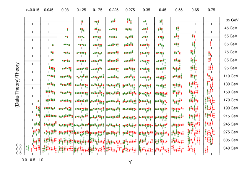
Figure 32: Comparison of HKN calculations with NuTeV data on $\nu$-Fe and $\bar{\nu}$-Fe cross sections [230].

According to the nCTEQ analysis [231], there are significant nuclear modification differences between charged-lepton DIS and neutrino ones. Our preliminary analysis also tends to obtain a result similar to the nCTEQ modifications which are different from the charged-lepton ones, especially in the region $x<0.4$. If it is true, we should be careful in calculating neutrino-nucleus cross sections in terms of the NPDFs determined mainly by the charged-lepton DIS measurements. So far, we take the same nuclear modifications for granted in discussing neutrino and charged-lepton DIS processes for nuclei. In the NPDF analyses of other groups (EPS, DSSZ) [223], there is no conspicuous difference, so that it is desirable to examine this issue by an independent analysis group. However, according to nCTEQ, the different results are caused by using different neutrino data sets. The nCTEQ used the raw cross section data while others used the corrected structure-function data.

We compare the cross sections data with the HKN calculations at the same kinematical points. For example, the comparison with the NuTeV data is shown in Fig. 32. Almost all the data are compatible with the HKN except that there are discrepancies at $x=0.015$ and 0.045 columns. These differences indicate that shallower shadowing effect is needed for explaining the NuTeV data. Actually, the shallow shadowing and suppression of the antishadowing effect are reported by the nCTEQ analysis [231]. On the other hand, the HKN parametrization seems to be consistent in the region $0.125\leq x\leq 0.55$, $E_{\nu}\leq 245$ GeV, so that nuclear modifications would be similar to the HKN ones in this medium-$x$ region. Therefore, if the neutrino data are included in the global analysis, the nuclear modifications could be rather different from the ones obtained mainly from the charged-lepton DIS at small $x$. Our analysis is in progress and more complete results will be reported elsewhere [230]. There is also an effort to compare the neutrino-$F_{2}$ data directly with the charged-lepton $F_{2}$ for the iron nucleus [232], and some differences seem to exist in the small-$x$ region ($x<0.05$).

Aside from this issue, the neutrino DIS experiment is in progress by the MINER$\nu$A collaboration [48] for various nuclei such as carbon, iron, and lead. They reported negative nuclear modifications at $0.05<x<0.15$ significantly larger than current expectations from typical simulations. It means that nuclear effects in neutrino DIS are much different from our understanding by the current NPDFs at $x\sim 0.1$. It is an interesting result to be investigated theoretically. At small $x$, the $W$ boson from the neutrino could propagate as axial-vector meson states in addition to vector meson ones, which causes a shadowing phenomena by multiple scattering of the mesons in a nucleus. Due to the additional axial-vector meson contributions, the shadowing could be different in the neutrino DIS from the one in the charged-lepton DIS. Although the MINER$\nu$A measurement at $x\sim 0.1$ is still not in the shadowing region, such an effect may influence phenomena in this region.

7.4 Neutrino-nucleus reactions at $Q^{2}\to 0$

Since the neutrino energies are of the order of 1-10 GeV for the current neutrino oscillation experiments, we need to have accurate neutrino cross sections in a wide kinematical range shown in Fig. 1. There is a region, $0<Q^{2}<1$ GeV² and $W^{2}\geq 4$ GeV², where both the DIS and resonance descriptions do not apply. Due to the condition $Q^{2}<1$ GeV², the cross section cannot be described by partons. It also cannot be described by nucleon resonances due to the condition $W^{2}\geq 4$ GeV². Before stepping into neutrino-nucleus reactions, we need to understand neutrino-nucleon reactions at $Q^{2}\to 0$.

In the next two paragraphs, we show that the neutrino cross sections at $Q^{2}\to 0$ are related to the pion-nucleon cross sections thanks to the partial conservation of the axial-vector current (PCAC). This observation will be a guidance to develop a model for the kinematical region in question. In general, the transverse ($T$) and longitudinal ($L$) structure functions are defined by corresponding total neutrino cross sections $\sigma_{T,\,L}$ as [233]

$$F_{T,\,L}(x,Q^{2}) =\frac{1}{\pi}\,\sqrt{1+Q^{2}/\nu^{2}}\,Q^{2}\,\sigma_{T,\,L}\,,$$

$$\sigma_{T,\,L} =\frac{(2\pi)^{4}}{4\sqrt{(p\cdot q)^{2}-p^{2}q^{2}}}\sum_{f}\delta^{\,(4)}(p+q-p_{f})\left|\,\langle\,f\,|\,\varepsilon_{T,\,L}\cdot J(0)\,|\,p\,\rangle\,\right|^{2},$$ (95)

where $\varepsilon_{T,\,L}$ is the polarization vector of $W$ or $Z$. In weak interactions, there are vector ($V$) and axial-vector ($A$) currents, which have transverse and longitudinal components. We know that the transverse cross section is finite at $Q^{2}=0$. From Eq. (95), this fact suggests that the transverse structure function should vanish ($F_{T}\to 0$) at $Q^{2}\to 0$.

The vector-current part of the hadron tensor should satisfy $q^{\,\mu}W_{\mu\nu}=0$ because the vector current is conserved. Therefore, the relation between the transverse and longitudinal ones ($F_{L}^{\,V}\sim Q^{2}F_{T}^{\,V}$) for the vector part is the same as the charged-lepton DIS. The axial-vector current is not conserved, so that a special attention needs to be paid at $Q^{2}\to 0$. It should be taken so as to satisfy the PCAC, $\partial_{\mu}\,A_{a}^{\,\mu}(x)=f_{\pi}\,m_{\pi}^{2}\,\pi_{a}(x)$, where $f_{\pi}$ is the pion-decay constant, $m_{\pi}$ is the pion mass, and $\pi_{a}(x)$ is the pion field with the isospin index $a$. The PCAC leads to the relation that the axial-vector part of the structure function is finite, and it is given by the pion-scattering cross section $\sigma_{\pi}$ as $F_{L}^{\,A}\to f_{\pi}^{\,2}\,\sigma_{\pi}/\pi$ at $Q^{2}\to 0$.

In order to describe the neutrino cross section in this region of $0<Q^{2}<1$ GeV² and $W^{2}\geq 4$ GeV², we need to express the structure functions by separating them into vector and axial-vector components. Then, we use the PCAC for the axial-vector part. However, the extrapolation of the structure functions into region $Q^{2}<1$ GeV² is not obvious, although they are known at $Q^{2}=0$. Considering experimental data, we may determine the $Q^{2}$ dependence with some theoretical guidance. We have not completed such an analysis at this stage. There were some studies, and Bodek and Yang [234], for example, supplied a widely-used model that is obtained by extending the DIS structure functions so as to be consistent with the data and the PCAC. However, a much simpler model without considering the PCAC is sometimes used, for example, in the FLUKA simulation [235] by taking $F_{2,\,3}(x,Q^{2})=(2Q^{2})/(Q_{0}^{2}+Q^{2})\,F_{2,\,3}(x,Q_{0}^{2})$. Further theoretical investigations in this kinematical region are highly called for. Particularly, the current studies in this kinematical region are restricted to the neutrino-nucleon interactions. Because we have information on nuclear structure functions $F_{2}^{A}$ and $F_{3}^{A}$, we should be able to estimate the neutrino-nucleus interactions and such theoretical efforts are needed.

8 Perspective

We have seen the latest development of neutrino-nucleus reaction models for the low-energy, QE, RES, and DIS regions; our own developments are particularly highlighted. Towards a unified description of the neutrino-nucleus reactions for all the relevant energy region, further developments are needed in each of the kinematical regions. To close the paper, we remark below possible future developments.

Few-body: The presented framework, correlated Gaussian combined with complex scaling method, would be applied to electron- and neutrino-induced reactions on light nuclei in the QE region. Implementation of a modern nuclear force including genuine three-body interaction will be important for more accurate descriptions of nuclear responses with various momentum transfer as suggested in Ref. [236]. It would also be interesting to study two-body current contributions. An ab initio calculation done with the Green’s function Monte Carlo method showed a rather large two-body current contributions [100]. An independent ab initio calculation is desired to evaluate possible uncertainties associated with theoretical models and calculational methods.

QE: It was shown that the inclusive electron scattering data in the QE region are well described with the impulse approximation scheme. In the scheme, the hole and particle propagations in nuclei are described by the nuclear spectral function, and FSI are accounted for by the the convolution method. On the other hand, the limitation of the approach is found in describing the dip region for which more mechanisms must be taken into account [12, 16, 199, 237, 238]. There are a large body of electron scattering data available over a broad range of energy and momentum transfer that can be used to test various mechanisms such as 2p2h, meson-exchange current, and transparency. The analysis of the electron scattering data can serve not only to determine the vector current part of the neutrino cross sections, but also to constrain the nuclear effects more stringently than the neutrino scattering data. In interpreting data from long-baseline neutrino oscillation experiments like T2K that mainly utilize low-energy neutrino beam ($E_{\nu}\ \raise 1.29167pt\hbox{$<$\kern-7.5pt\lower 4.30554pt\hbox{$\sim$}}\$ 1 GeV), a solid understanding of the CCQE(-like) processes is essential. Therefore, only theoretical models that have been validated by the electron scattering data should be used in analyzing the data.

RES: There are still remaining issues in the elementary neutrino-nucleon reaction amplitudes. All models have used cross section data for the elementary single pion production processes measured in the bubble-chamber experiments [25, 73], in order to fix the axial coupling for the $N$-$\Delta(1232)$ transition. However, the experiments used the deuterium target and, as discussed in Ref. [74] and Sec. 6.1, the FSI could be important to extract the elementary-process cross sections from the data although it was neglected in the published analyses [25, 73]. Thus it will be important to extend the analysis of Ref. [74] to analyze the bubble-chamber data to extract the elementary cross sections, and this is currently underway. Another issue is $Q^{2}$ dependence of axial $N$-$N^{*}$ form factors for higher resonances beyond $\Delta(1232)$. Although the $Q^{2}$ dependence has been assumed to be a dipole form with the axial mass of $\sim$ 1 GeV, this could be improved for $N^{*}$ near the DIS region by matching the structure functions of the DCC model with those calculated with the nucleonic PDF in the region where the RES and DIS regions are overlapping; $W\sim$ 2 GeV and $Q^{2}>$ 1 GeV². This matching can be done with the DCC model because the model includes $\pi\pi N$ channel that would give a dominant contribution in this region.

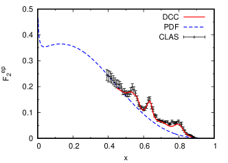
Figure 33: (Color online) $F_{2}$ for the inclusive electron-proton scattering at $Q^{2}=2.425~{}{\rm GeV}^{2}$ calculated with the DCC model (red solid curve) and with the nucleonic PDF (blue dashed curve). The horizontal axis is Bjorken scaling variable $x$. The data are from Ref. [239].

Actually, as shown in Fig. 33, the DCC model and the nucleonic PDF are already reasonably consistent for the vector (electromagnetic) current at $x\sim 0.45$ (where $W\sim$ 2 GeV), because both of them have been fitted to relevant inclusive electron scattering data. We expect a result similar to Fig. 33 can also be achieved for the axial current by adjusting the $N$-$N^{*}$ form factors in the DCC model. In future, lattice QCD will be able to provide us with information on the axial vector response of the nucleon in the RES region, and this LQCD-based input will be implemented in the reaction model [72].

Next important task is to construct a neutrino-nucleus reaction model in the RES region using the DCC elementary amplitudes as a building block. In the $\Delta(1232)$ region, a quantum mechanical description is possible with the $\Delta$-hole model [170, 171, 172, 173]. As discussed in Sec. 6.2, we have developed such a model for the coherent pion productions. It would be desirable to apply the method also to incoherent pion productions that are relevant to the T2K experiment. The DCC amplitudes should also be a reasonable input for a neutrino-nucleus reaction model for the whole resonance region, and this development should be pursued. It is worth emphasizing again that the DCC model is the only available model that provides: (i) two-pion production amplitudes with all the resonance contributions taken into account; (ii) the well-controlled interference between the resonance and non-resonance contributions.

DIS: The NPDFs should be determined by including neutrino DIS data. In particular, the issue of the difference between the nuclear modifications of charged-lepton DIS and neutrino DIS should be clarified. Furthermore, experimental information from LHC needs to be considered and it could constrain the NPDFs in a small-$x$ region. Experimental efforts are in progress to measure the nuclear modification in neutrino DIS by the MINER$\nu$A collaboration. Its data will provide new information in the anti-shadowing region. Because axial-vector mesons contribute to the shadowing in the neutrino DIS in addition to vector mesons according to the vector-meson-dominance model, shadowing could be different for neutrino DIS from the one for charged-lepton DIS. Such effects could affect the nuclear modifications in the neighboring anti-shadowing region. Therefore, the shadowing and anti-shadowing phenomena should be interesting theoretical topics that can be studied with future neutrino measurements. Next, a model needs to be developed in the small $Q^{2}$($<1$ GeV²) region with large $W^{2}$($>4$ GeV²). Because this region cannot be described solely by DIS models or resonance models, simple empirical models have been used. However, such studies are so far only for the neutrino-nucleon interactions, and a realistic model for the neutrino-nuclear interactions should be developed by taking into account proper nuclear modifications.

References

- [1] K.A. Olive et al. (Particle Data Group), Chin. Phys. C 38, 090001 (2014).
- [2] M. C. Gonzalez-Garcia, M. Maltoni, and T. Schwetz, Nucl. Phys. B908, 199 (2016).
- [3] F. Capozzi, G. L. Fogli, E. Lisi, A. Marrone, D. Montanino, and A. Palazzo, Phys. Rev. D 89, 093018 (2014).
- [4] D. V. Forero, M. Tortola, and J. W. F. Valle, Phys. Rev. D 90, 093006 (2014).
- [5] K. Abe et al., arXiv:1109.3262.
- [6] K. Abe et al., Prog. Theor. Exp. Phys. 2015 053C02, (2015).
- [7] R. Acciarri et al. (DUNE Collaboration), arXiv:1512.06148.
- [8] K. Abe et al. (T2K Collaboration), Phys. Rev. D 91, 072010 (2015).
- [9] K. Abe et al. (T2K Collaboration), arXiv:1609.04111.
- [10] H. Gallagher, G. Garvey and G. P. Zeller, Ann. Rev. Nucl. Part. Sci. 61, 355 (2011).
- [11] J.A. Formaggio and G.P. Zeller, Rev. Mod. Phys. 84, 1307 (2012).
- [12] L. Alvarez-Ruso, Y. Hayato and J. Nieves, New J. Phys. 16, 075015 (2014).
- [13] G. T. Garvey, D. A. Harris, H. A. Tanaka, R. Tayloe, and G. P. Zeller, Phys. Rep. 580, 1 (2015).
- [14] O. Benhar, P. Huber, C. Mariani, and D. Meloni, arXiv:1501.06448.
- [15] U. Mosel, Ann. Rev. Nucl. Part. Sci. 66, 171 (2016).
- [16] T. Katori and M. Martini, arXiv:1611.07770.
- [17] Y. Hayato, Acta Phys. Polon. B40, 2477 (2009).
- [18] C. Andreopoulos et al., Nucl. Instrum. Meth. A614, 87 (2010).
- [19] T. Golan, J.T. Sobczyk, and J. Zmuda, Nucl. Phys. Proc. Suppl. 229-232, 499 (2012).
- [20] O. Buss, T. Gaitanos, K. Gallmeister, H. van Hees, M. Kaskulov, O. Lalakulich, A.B. Larionov, T. Leitner, J. Weil, and U. Mosel, Phys. Rept. 512, 1 (2012).
- [21] S. X. Nakamura et al., AIP Conf. Proc. 1663 120010 (2015); http://nuint.kek.jp/index_e.html.
- [22] S. J. Barish et al., Phys. Rev. D 16, 3103 (1977).
- [23] G. M. Radecky et al., Phys. Rev. D 25, 1161 (1982); Erratum: [Phys. Rev. D 26, 3297 (1982)].
- [24] N. J. Baker et al., Phys. Rev. D 23, 2499 (1981).
- [25] T. Kitagaki et al., Phys. Rev. D 34, 2554 (1986).
- [26] D. Allasia et al., Nucl. Phys. B343, 285 (1990).
- [27] T. Kitagaki et al., Phys. Rev. D 28, 436 (1983).
- [28] A. Kayis-Topaksu et al. (CHORUS), Eur. Phys. J. C51, 775 (2007).
- [29] Q. Wu et al. (NOMAD), Phys. Lett. B660, 19 (2008).
- [30] J. P. Berge et al., Z. Phys. C49, 187 (1991).
- [31] Un-Ki Yang et al. (CCFR/NuTeV), Phys. Rev. Lett. 86, 2742 (2001).
- [32] B. T. Fleming et al. (CCFR), Phys. Rev. Lett. 86, 5430 (2001).
- [33] A. Bodek et al. (CCRF/NuTeV), Int. J. Mod. Phys. A16, 202 (2001).
- [34] R. Gran et al. (K2K Collaboration), Phys. Rev. D 74, 052002 (2006).
- [35] M. Hasegawa et al. (K2K Collaboration), Phys. Rev. Lett. 95, 252301 (2005).
- [36] A. Bodek and U. K. Yang, Nucl. Phys. Proc. Suppl. 112, 70 (2002).
- [37] A. A. Aguilar-Arevalo et al. (MiniBooNE Collaboration), Phys. Rev. D 81, 092005 (2010).
- [38] A. A. Aguilar-Arevalo et al. (MiniBooNE Collaboration), Phys. Rev. D 88, 032001 (2013).
- [39] P. Adamson et al. (MINOS Collaboration), Phys. Rev. D 91, 012005 (2015).
- [40] P. A. Rodrigues et al. (MINERA Collaboration), Phys. Rev. Lett. 116, 071802 (2016).
- [41] S. Nakayama et al. (K2K Collaboration), Phys. Lett. B619, 255 (2005).
- [42] A. A. Aguilar-Arevalo et al. (MiniBooNE Collaboration), Phys. Rev. D 81, 013005 (2010).
- [43] A. A. Aguilar-Arevalo et al. (MiniBooNE Collaboration), Phys. Rev. D 83, 052007 (2011).
- [44] B. Eberly et al. (MINERA Collaboration), Phys. Rev. D 92, 092008 (2015).
- [45] K. Hiraide et al. (SciBooNE Collaboration), Phys. Rev. D 78, 112004 (2008).
- [46] D. Rein and L. M. Sehgal, Nucl. Phys. B223, 29 (1983).
- [47] A. Higuera et al. (MINERA Collaboration), Phys. Rev. Lett. 113, 261802 (2014).
- [48] J. Mousseau et al. (MINERA Collaboration), Phys. Rev. D 93, 071101(R) (2016).
- [49] J. D. Walecka, Muon Physics II, 114 (Editors V. W. Hughes and C. S. Wu, Academic Press, NY, 1975)
- [50] S. Nakamura, T. Sato, V. Gudkov, and K. Kubodera, Phys. Rev. C 63, 034617 (2001).
- [51] M. Day and K. S. McFarland, Phys. Rev. D 86, 053003 (2012).
- [52] V. Bernard et al., J. Phys. G28, R1 (2002).
- [53] A. A. Aguilar-Arevalo et al. (MiniBooNE Collaboration), Phys. Rev. D 82, 092005 (2010).
- [54] A. A. Aguilar-Arevalo et al. (MiniBooNE Collaboration), Phys. Rev. D 91, 012004 (2015).
- [55] A. M. Ankowski, O. Bengar, T. Mori, R. Yamaguchi, and M. Sakuda, Phys. Rev. Lett. 108, 052505 (2012).
- [56] T. J. Hobbs, M. Alberg, and G. A. Millter, Phys. Rev. C 93, 052801(R) (2016).
- [57] E. A. Paschos and D. Schalla, Adv. High Energy Phys. 2013, 270792 (2013).
- [58] S. L. Adler, Ann. Phys. 50, 189 (1968).
- [59] O. Lalakulich, E. A. Paschos, and G. Piranishvili, Phys. Rev. D 74, 014009 (2006).
- [60] E. Hernández, J. Nieves, and M. Valverde, Phys. Rev. D 76, 033005 (2007).
- [61] E. Hernández, J. Nieves, M. Valverde, and M. J. Vicente Vacas, Phys. Rev. D 81, 085046 (2010).
- [62] B. D. Serot and X. Zhang, Advances in Quantum Field Theory, ed. by Sergey Ketov (Intech, Rijeka, Croatia, 2012); arXiv:1110.2760.
- [63] B. D. Serot and X. Zhang, Phys. Rev. C 86, 015501 (2012).
- [64] T. Leitner, O. Buss, L. Alvarez-Ruso, and U. Mosel, Phys. Rev. C 79, 034601 (2009).
- [65] T. Sato, D. Uno, and T.-S. H. Lee, Phys. Rev. C 67, 065201 (2003).
- [66] K. Matsui, T. Sato, and T.-S. H. Lee, Phys. Rev. C 72, 025204 (2005).
- [67] S.X. Nakamura, H. Kamano, and T. Sato, Phys. Rev. D 92, 074024 (2015).
- [68] J. Liu, N. C. Mukhopadhyay, and L. Zhang, Phys. Rev. C 52, 1630 (1995).
- [69] T. R. Hemmert, B. R. Holstein, and N. C. Mukhopadhyay, Phys. Rev. D 51, 158 (1995).
- [70] L. S. Geng, J. M. Camalich, L. Alvarez-Ruso, and M. J. Vicent Vacas, Phys. Rev. D 78, 014011 (2008).
- [71] M. Procura, Phys. Rev. D 78, 094021 (2008).
- [72] C. Alexandrou, G. Koutsou, J. W. Negele, Y. Proestos, and A. T. Tsapalis, Phys. Rev. D 83, 014501 (2011).
- [73] S. J. Barish et al., Phys. Rev. D 19, 2521 (1979).
- [74] J.-J. Wu, T. Sato, and T.-S. H. Lee, Phys. Rev. C 91, 035203 (2015).
- [75] R. D. Field, Application of Perturbative QCD, (Addison-Wesley Publishing Company, Inc., 1989); E. Leader and E. Predazzi, An Introduction to Gauge Theories and Modern Particle Physics (Cambridge University, 1996); R. Devenish and A. Cooper-Sarkar, Deep Inelastic Scattering (Oxford University Press, 2004); Section “Structure Functions” in K. A. Olive et al. (Particle Data Group), Chin. Phys. C 38, 090001 (2014).
- [76] R. K. Ellis, W. J. Stirling, and B. R. Webber, QCD and Collider Physics (Cambridge University, 1996).
- [77] L. W. Withlow et al., Phys. Lett. B250, 193 (1990); K. Abe et al. (E143 Collaboration), Phys. Lett. B452, 194 (1999).
- [78] Information of nucleonic PDFs is provided at http://hepdata.cedar.ac.uk/pdf/pdf3.html.
-
[79]
H. Kamano, S.X. Nakamura, T.-S.H. Lee, and T. Sato,
Phys. Rev. C 88, 035209 (2013);
H. Kamano, S.X. Nakamura, T.-S.H. Lee, and T. Sato, Phys. Rev. C 94, 015201 (2016). - [80] D. Rein and L. M. Sehgal, Annals Phys. 133, 79 (1981).
- [81] D. Rein, Z. Phys. C 35, 43 (1987).
- [82] M. Kobayashi, T. Sato, and H. Ohtsubo, Prog. Theor. Phys. 98, 927 (1997).
- [83] T. Sato and T.-S. H. Lee, Phys. Rev. C 54, 2660 (1996).
- [84] H. Kamano, Phys. Rev. C 88, 045203 (2013).
- [85] K. Joo et al. (CLAS Collaboration), Phys. Rev. Lett. 88, 122001 (2002).
- [86] Preliminary results from JLab E00-002, C. Keppel, M.I. Niculescu, spokespersons. Data files can be obtained at https://hallcweb.jlab.org/resdata/database.
- [87] C. Wilkinson, P. Rodrigues, S. Cartwright, L. Thompson, and K. McFarland, Phys. Rev. D 90, 112017 (2014).
- [88] D. Day et al., Phys. Rev. D 28, 2714 (1983).
- [89] S. N. Biswas, S. R. Choudhury, A. K. Goyal and J. N. Passi, Phys. Rev. D 18, 3187 (1978).
- [90] S. A. Adjei, D. A. Dicus, and V. L. Teplitz, Phys. Rev. D 24, 623 (1981).
- [91] E. Hernández, J. Nieves, S.K. Singh, M. Valverde, and M.J. Vicente Vacas Phys. Rev. D 77, 053009 (2008).
- [92] H. A. Bethe and J. R. Wilson, Astrophys. J. 295, 14 (1985).
- [93] K. G. Balasi, K. Langanke, and G. Martinez-Pinedo, Prog. Part. Nucl. Phys. 85, 33 (2015).
- [94] W. C. Haxton, Phys. Rev. Lett. 60, 1999 (1988).
- [95] S. X. Nakamura, K. Sumiyoshi, and T. Sato, Phys. Rev. C80, 035802 (2009).
- [96] S. Nasu, S.X. Nakamura, K. Sumiyoshi, T. Sato, F. Myhrer, and K. Kubodera, Astrophys. J. 801, 78 (2015).
- [97] S. E. Woosley, D. H. Hartmann, R. D. Hoffman, and W. C. Haxton, Astrophys. J. 356, 272 (1990).
- [98] T. Suzuki, S. Chiba, T. Yoshida, T. Kajino and T. Otsuka, Phys. Rev. C 74, 034307 (2006).
- [99] T. Yoshida, T. Kajino, H. Yokomakura, K. Kimura, A. Takamura, D.H. Hartmann, Phys. Rev. Lett. 96, 091101 (2006).
- [100] A. Lovato, S. Gandolfi, J. Carlson, S.C. Pieper, R. Schiavilla Phys. Rev. C 91, 062501 (2015); Phys. Rev. Lett. 117, 082501 (2016).
- [101] S. Nakamura, T. Sato, S. Ando, T. -S. Park, F. Myhrer, V. Gudkov, and K. Kubodera, Nucl. Phys. A707, 561 (2002).
- [102] K. Tamura, T. Niwa, T. Sato, and H. Ohtsubo, Nucl. Phys. A536, 597 (1992).
- [103] T. Sato, T. Niwa, and H. Ohtsubo, in Proc. of IVth Int. Symp. on Weak and Electromagnetic Interaction in Nuclei, ed. H. Ejiri, T. Kishimoto, and T. Sato (Singapore: World Scientific 1995), 488
- [104] M. Doi, T. Sato, H. Ohtsubo, and M. Morita, Nucl. Phys. A511, 507 (1990).
- [105] K. Kubodera and T.-S. Park, Ann. Rev. Nucl. Part. Sci. 54, 19 (2004).
-
[106]
M. Butler and J. W. Chen, Nucl. Phys. A675, 575 (2000);
M. Butler, J. W. Chen, and X. Kong, Phys. Rev. C 63, 035501 (2001). - [107] L. E. Marucci, R. Schiavilla, and M. Viviani, Phys. Rev. Lett. 110, 192503 (2013).
- [108] G. Shen, L. E.Marucci, J. Carlson, S. Gandolfi, R. Schiavilla, Phys. Rev. C 86, 035503 (2012).
- [109] J. Golak, R. Skibinski, H. Witala, W. Glöckle, A. Nogga and H. Kamada, Phys. Rep. 415, 89 (2005).
- [110] S. Bacca and S. Pastore, J. Phys. G41, 123002 (2014).
- [111] D. Gazit and N. Barnea, Phys. Rev. Lett. 98, 192501 (2007).
- [112] E. O’Conner, D. Gazit, C. J. Horowitz, A. Schwenk, and N. Barnea, Phys. Rev. C 75, 055803 (2007).
- [113] A. Lovato, S. Gandolfi, J. Carlson, S. C. Pieper, and R. Schiavilla, Phys. Rev. C 91, 062501 (2015).
- [114] J. Carlson, G. Gandolfi, F. Pederiva, S. C. Pieper, R. Schiavilla, K. E. Schmidt, and R. B. Wiringa, Rev. Mod. Phys. 87, 1067 (2015).
- [115] W. Horiuchi and Y. Suzuki, Phys. Rev. C 87, 034001 (2013).
- [116] N. Moiseyev, Phys. Rep. 302, 211 (1998).
- [117] S. Aoyama, T. Myo, K. Kato, and K. Ikeda, Prog. Theor. Phys. 116, 1 (2006).
- [118] K. Varga and Y. Suzuki, Phys. Rev. C 52, 2885 (1995).
- [119] Y. Suzuki and K. Varga, Stochastic Variational Approach to Quantum-Mechanical Few-Body Problems, Lecture Notes in Physics Monographs Vol. m54 (Springer Berlin, 1998).
- [120] Y. Suzuki, W. Horiuchi, M. Orabi, and K. Arai, Few-Body Syst. 42, 33 (2008).
- [121] H. Kamada et al., Phys. Rev. C 64, 044001 (2001).
- [122] H. Feldmeier, W. Horiuchi, T. Neff, and Y. Suzuki, Phys. Rev. C 84, 054003 (2011).
- [123] W. Horiuchi and Y. Suzuki, Phys. Rev. C 89, 011601(R) (2014).
- [124] Y. Suzuki and W. Horiuchi, World Scientific Review Volume “Emergent phenomena in Atomic Nuclei from Large-scale Modeling: a Symmetry-guided Perspective”, Chapter 7, 173 (2016).
- [125] J. Mitroy, S. Bubin, W. Horiuchi, Y. Suzuki, L. Adamowicz, W. Cencek, K. Szalewicz, J. Komasa, D. Blume, and K. Varga, Rev. Mod. Phys. 85, 693 (2013).
- [126] S. Aoyama, K. Arai, Y. Suzuki, P. Descouvemont, and D. Baye, Few-Body Syst. 52, 97 (2012).
- [127] B. S. Pudliner, V. R. Pandharipande, J. Carlson, S. C. Pieper, and R. B. Wiringa, Phys. Rev. C 56, 1720 (1997).
- [128] E. Hiyama, B. F. Gibson, and M. Kamimura, Phys. Rev. C 70, 031001(R) (2004).
- [129] D. R. Tilley, H. R. Weller, and G. M. Hale, Nucl. Phys. A541, 1 (1992).
- [130] W. Horiuchi and Y. Suzuki, Phys. Rev. C 78, 034305 (2008).
- [131] W. Horiuchi and Y. Suzuki, Few-Body Syst. 54, 2407 (2013).
- [132] W. Horiuchi, Y. Suzuki, and K. Arai, Phys. Rev. C 85, 054002 (2012).
- [133] T. Shima et al., Phys. Rev. C 72, 044004 (2005).
- [134] S. Nakayama et al., Phys. Rev. C 76, 021305(R) (2007).
- [135] P. Ring and P. Schuck, The Nuclear Many-Body Problem, Texts and Monographs in Physics (Springer, New York, 1980).
- [136] Yu. M. Arkatov et al., Yad. Konst. 4, 55 (1979).
- [137] D. Gazit, S. Bacca, N. Barnea, W. Leidemann, and G. Orlandini, Phys. Rev. Lett. 96, 112301 (2006).
- [138] S. Quaglioni and P. Navrátil, Phys. Lett. B652, 370 (2007).
- [139] D. P. Wells et al., Phys. Rev. 46, 449 (1992).
- [140] T. Shima (private communication).
- [141] T. Yoshida et al., Astrophys. J. 686, 448 (2008).
- [142] E. K. Warburton and B. A. Brown, Phys. Rev. C 46, 923 (1992).
- [143] D. J. Millener and D. Kurath, Nucl. Phys. A255, 315 (1975). B. A. Brown et al. OXBASH, the Oxford, Buenos-Aires, Michigan State Shell Model Program.
- [144] K. Koshigiri, H. Ohtsubo, and M. Morita, Prog. Theor. Phys. 62, 706 (1979).
- [145] O. Benhar, N. Farina, H. Nakamura, M. Sakuda, and R. Seki, Phys. Rev. D 72, 053005 (2005).
- [146] O. Benhar, Phys. Rev. C 87, 024606 (2013).
- [147] A. Ankowski, O. Benhar and M. Sakuda, Phys. Rev. D 91, 033005 (2015); Supplemental Materials.
- [148] A.M. Ankowski, O. Benhar, and N. Farina, Phys. Rev. D 82, 013002 (2010).
- [149] R.A. Smith and E.J Moniz, Nucl. Phys. B43, 605 (1972).
- [150] O. Benhar, A. Fabrocini, S. Fantoni, and I. Sick, Nucl. Phys. A579, 493 (1994).
- [151] S. Turck-Chièze, Lecture Notes in Physics 137, 251 (1981).
- [152] S.C. Pieper, R.B. Wiringa, and V.R. Pandharipande, Phys. Rev. C 46, 1741 (1992).
- [153] NuInt12: Proceedings of The 8th International Workshop on Neutrino-Nucleus Interactions In The Few-GeV Region, 22-27 October, 2012, Rio de Janeiro, Brasil, AIP. Conf. Proc. 1663, 1 (2015), Edited by Helio da Motta, Jorge G. Morfin and Makoto Sakuda
- [154] O. Benhar, D. Day, and I. Sick, Rev. Mod. Phys. 80, 189 (2008).
- [155] Y. Horikawa, F. Lenz, and N.C. Mukhopadhyay, Phys. Rev. C 22, 1680 (1980).
- [156] D. Rohe et al. (JLAB E97-006 Collaboration), Phys. Rev. C 72, 054602 (2005).
- [157] E. D. Cooper, S. Hama, B. C. Clark, and R. L. Mercer, Phys. Rev. C 47, 297 (1993).
- [158] H. de Vries, C. W. de Jager, and C. de Vries, At. Data Nucl. Data Tables 36, 495 (1987).
- [159] J.J. Kelly, Phys. Rev. C 66, 065203 (2002).
- [160] P. Barreau et al., Nucl. Phys. A402, 515 (1983).
- [161] D.T. Baran et al., Phys. Rev. Lett. 61, 400 (1988).
- [162] R.R. Whitney, I. Sick, J.R. Ficenec, R.D. Kephart, and W.P. Trower, Phys. Rev. C 9, 2230 (1974).
- [163] W. M. Alberico, M. Ericson, and A. Molonari, Ann. Phys.(N.Y.) 154, 356 (1984).
- [164] A. Gil, J. Nieves, and E. Oset, Nucl. Phys. A627, 543 (1997).
- [165] J. Nieves, talk at Neutrino 2016, London, July 2016.
- [166] N. Rocco, A. Lovato, and O. Benhar, Phys. Rev. Lett 116, 192501 (2016).
- [167] A. Aguilar-Arevalo et al. (MiniBooNE Collaboration), Phys. Rev. D 83, 052009 (2011).
- [168] T. Le et al. (MINERA Collaboration), Phys. Lett. B749, 130 (2015).
- [169] A. Kerman, H. McManus, and R. Thaler, Ann. Phys. 8, 551 (1959).
- [170] L. S. Kisslinger, W. L. Wang, Annals Phys. 99, 374 (1976).
- [171] M. Hirata, F. Lenz and K. Yazaki, Annals Phys. 108, 116 (1977).
- [172] M. Hirata, J.H. Koch, E. J. Moniz, and F. Lenz, Annals Phys. 120, 205 (1979).
- [173] S. Taniguchi, T. Sato and H. Ohtsubo, Prog. Theor. Phys. 102, 333 (1999).
- [174] O. Lalakulich and U. Mosel, Phys. Rev. C 87, 014602 (2013).
- [175] E. Hernández, J. Nieves, and M. J. Vicente Vacas, Phys. Rev. D 87, 113009 (2013).
- [176] A.A. Aguilar-Arevalo et al. (MiniBooNE Collaboration), Phys. Lett. B664, 41 (2008).
- [177] Y. Kurimoto et al. (SciBooNE Collaboration), Phys. Rev. D 81, 111102 (2010).
- [178] P. Allen et al., Nucl. Phys. B264, 221 (1986).
- [179] E. A. Paschos, Ji-Young Yu and M. Sakuda, Phys. Rev. D 69, 014013 (2004).
- [180] M. O. Wascko (MiniBooNE Collaboration), Nucl. Phys. B, Proc. Suppl. 159, 50 (2006).
- [181] K. M. Graczyk, D. Kielczwska, P. Przewloski and J. T. Sobczyk, Phys. Rev. D 80, 093001 (2009).
- [182] P. Rodrigues, C. Wilkinson and K. McFarland, Eur. Phys. J. C 76, 474 (2016).
- [183] E. M. Darwish, H. Arenhövel and M. Schwamb, Eur. Phys. J. A 16, 111 (2003).
- [184] A. Fix and H. Arenhövel, Phys.Rev. C 72, 064005 (2005).
- [185] M. I. Levchuk, A. Yu. Loginov, A. A. Sidorov, V. N. Stibunov and M. Schumacher, Phys. Rev. C 74, 014004 (2006).
- [186] M. Schwamb, Phys. Rep. 485, 109 (2010).
- [187] T. Sato and T.-S. H. Lee, Phys. Rev. C 63, 055201 (2001).
- [188] R. Machleidt, in Advances in Nuclear Physics, edited by J.W. Negele and E. Vogt (Plenum, New York, 1989), Vol.19, Chap. 2.
- [189] D. Rein and L. M. Sehgal, Phys. Lett. B657, 207 (2007).
- [190] E. Hernández, J. Nieves, and M.J. Vicente-Vacas, Phys. Rev. D 80, 013003 (2009).
- [191] E.A. Paschos, A. Kartavtsev and G.J. Gounaris, Phys. Rev. D 74, 054007 (2006).
- [192] Ch. Berger and L.M. Sehgal, Phys. Rev. D 79, 053003 (2009).
- [193] E. A. Paschos and D. Schalla, Phys. Rev. D 80, 033005 (2009).
- [194] N.G. Kelkar, E. Oset, and P. Fernandez de Cordoba, Phys. Rev. C 55, 1964 (1997).
- [195] S. K. Singh, M. S. Athar, and S. Ahmad, Phys. Rev. Lett. 96, 241801 (2006).
- [196] L. Alvarez-Ruso, L.S. Geng, S. Hirenzaki, and M.J. Vicente Vacas, Phys. Rev. C 75, 055501 (2007); 80, 019906(E) (2009).
- [197] L. Alvarez-Ruso, L.S. Geng, and M.J. Vicente Vacas, Phys. Rev. C 76, 068501 (2007); 80, 029904(E) (2009).
- [198] J.E. Amaro, E. Hernández, J. Nieves and M. Valverde, Phys. Rev. D 79, 013002 (2009).
- [199] M. Martini, M. Ericson, G. Chanfray, and J. Marteau, Phys. Rev. C 80, 065501 (2009).
- [200] S.X. Nakamura, T. Sato, T.-S.H. Lee, B. Szczerbinska, and K. Kubodera, Phys. Rev. C 81, 035502 (2010).
- [201] E. Hernández, J. Nieves, and M. Valverde, Phys. Rev. D 82, 077303 (2010).
- [202] S.X. Nakamura, J. Phys. Conf. Ser. 408, 012043 (2013).
- [203] B. Karaoglu and E. J. Moniz, Phys. Rev. C 33, 974 (1986).
- [204] M. Blecher et al., Phys Rev. C 20, 1884 (1979).
- [205] F. Binon, P. Duteil, J. P. Garron, J. Gorres, L. Hugon, J. P. Peigneux, C. Schmit, M. Spighel and J. P. Stroot, Nucl. Phys. B17, 168 (1970).
- [206] R. Gothe et al., Phys. Lett. B355, 59 (1995).
- [207] B. Krusche et al., Phys. Lett. B526, 287 (2002).
- [208] M. H. Ahn et al., Phys. Rev. D 74, 072003 (2006).
- [209] K. Abe et al. (T2K Collaboration), Phys. Rev. Lett. 117, 192501 (2016).
-
[210]
K. Abe et al. (T2K Collaboration),
Phys. Rev. D 87, 012001 (2013);
http://t2k-experiment.org/results/neutrino-beam-flux-2013. - [211] J. L. Raaf, PhD thesis, University of Cincinnati, FERMILAB-THESIS-2007-20 (2005).
- [212] A.A. Aguilar-Arevalo et al. (MiniBooNE Collaboration), Phys. Rev. D 79, 072002 (2009).
- [213] J. J. Aubert et al. (European Muon Collaboration), Phys. Lett. B123, 275 (1983).
- [214] D. F. Geesaman, K. Saito, and A. W. Thomas, Ann. Rev. Nucl. Part. Sci. 45, 337 (1995); L. Frankfurt, V. Guzey, and M. Strikman, Phys. Rept. 512, 255 (2012); V. Barone and E. Predazzi, High-energy particle diffraction (Springer, 2001).
- [215] T. Uchiyama and K. Saito, Phys. Rev. C 38, 2245 (1988); M. Ericson and S. Kumano, Phys. Rev. C 67, 022201 (2003); M. Hirai, S. Kumano, K. Saito, and T. Watanabe, Phys. Rev. C 83, 035202 (2011).
- [216] K. Saito and A. W. Thomas, Nucl. Phys. A574, 659 (1994); I. C. Cloet, W. Bentz, and A. W. Thomas, Phys. Rev. Lett. 95, 052302 (2005).
- [217] M. Hirai, S. Kumano, and T. -H. Nagai, Phys. Rev. C 76, 065207 (2007); 70, 044905 (2004); M. Hirai, S. Kumano, M. Miyama, Phys. Rev. D 64, 034003 (2001).
- [218] S. Kumano, Phys. Rev. D 66, 111301 (2002); M. Hirai, S. Kumano, and T.-H. Nagai, Phys. Rev. D 71, 113007 (2005); I .C. Cloet, W. Bentz, and A. W. Thomas, Phys. Rev. Lett. 102, 252301 (2009); W. Bentz et al., Phys. Lett. B693, 462 (2010).
- [219] H. Mineo, W. Bentz, N. Ishii, A. W. Thomas, and K. Yazaki, Nucl. Phys. A735, 482 (2004); I. C. Cloet, W. Bentz, and A. W. Thomas, Phys. Lett. B642, 210 (2006); Phys. Rev. Lett. 109, 182301 (2012).
- [220] S. Kumano, Phys. Lett. B342, 339 (1995).
- [221] S. Kumano, Phys. Rept. 303, 183 (1998); G. T. Garvey and J.-C. Peng, Prog. Part. Nucl. Phys. 47, 203 (2001); J.-C. Peng and J.-W. Qiu, Prog. Part. Nucl. Phys. 76, 43 (2014).
- [222] M. Miyama and S. Kumano, Comput. Phys. Commun. 94, 185 (1996). See also M. Hirai et al., Comput. Phys. Commun. 108, 38 (1998); 111, 150 (1998); 183, 1002 (2012).
- [223] K.J. Eskola, H. Paukkunen, and C.A. Salgado, JHEP 04, 065 (2009); H. Paukkunen and C.A. Salgado, JHEP 1007, 032 (2010); Phys. Rev. Lett. 110, 212301 (2013); D. de Florian, R. Sassot, P. Zurita, and M. Stratmann, Phys. Rev. D 85, 074028 (2012); K. Kovarik et al., Phys. Rev. D 93, 085037 (2016); See also L. Frankfurt, V. Guzey, and M. Strikman, Phys. Rept. 512, 255 (2012).
- [224] V. Guzey et al., Phys. Lett. B726, 290 (2013); JHEP 1310, 207 (2013); Eur. Phys. J. C 74, 2942 (2014).
- [225] I. Helenius, H. Paukkunen, and K. J. Eskola, PoS DIS2015, 036 (2015).
- [226] For the Fermilab E-906/SeaQuest experiment, see http://www.phy.anl.gov/mep/drell-yan/.
- [227] Parity-Violating EMC Experiment, Proposal PR12-14-007 to JLab PAC-42 (2014).
- [228] M. Tzanov, et al. (NuTeV Collaboration), Phys. Rev D 74, 012008 (2006).
- [229] G. Önengüt et al. (CHORUS Collaboration), Phys. Lett. B632, 65 (2006).
- [230] M. Hirai, JPS Conf. Proc. 12, 010024 (2016); M. Hirai, S. Kumano, and K. Saito, research in progress.
- [231] I. Schienbein et al., Phys. Rev. D 77, 054013 (2008); 80, 094004 (2009); K. Kovarik et al., Phys. Rev. Lett. 106, 122301 (2011).
- [232] N. Kalantarians, talk at the 10th International Workshop on Neutrino-Nucleus Interactions in the Few-GeV Region, Osaka, Japan, Nov. 16-21, 2015.
- [233] A. Donnachie and P. V. Landshoff, Z. Phys. C 61, 139 (1994); B. Z. Kopeliovich, Nucl. Phys. B139, 219 (2005); S. A. Kulagin and R. Petti, Phys. Rev. D 76, 094023 (2007).
- [234] A. Bodek and U.-K. Yang, arXiv:1011.6592.
- [235] G. Battistoni et al., Acta Phys. Pol. B 40, 2431 (2009); see http://www.fluka.org for the FLUKA package.
- [236] S. Bacca, N. Barnea, W. Leidemann, and G. Orlandini, Phys. Rev. Lett. 102, 162501 (2009).
- [237] M. Martini, M. Ericson, and G. Chanfray, Phys. Rev. D 85, 093012 (2012); 87, 013009 (2013).
- [238] J. Nieves, F. Sanchez, I. Ruiz Simo, and M.J. Vicente Vacas, Phys. Rev. D 85, 113008 (2012).
- [239] M. Osipenko et al., CLAS-NOTE-2003-001; hep-ex/0309052.