Learning Optimal Parameters for Multi-target Tracking with Contextual Interactions

Abstract

We describe an end-to-end framework for learning parameters of min-cost flow multi-target tracking problem with quadratic trajectory interactions including suppression of overlapping tracks and contextual cues about co-occurrence of different objects. Our approach utilizes structured prediction with a tracking-specific loss function to learn the complete set of model parameters. In this learning framework, we evaluate two different approaches to finding an optimal set of tracks under a quadratic model objective, one based on an LP relaxation and the other based on novel greedy variants of dynamic programming that handle pairwise interactions. We find the greedy algorithms achieve almost equivalent accuracy to the LP relaxation while being up to 10x faster than a commercial LP solver. We evaluate trained models on three challenging benchmarks. Surprisingly, we find that with proper parameter learning, our simple data association model without explicit appearance/motion reasoning is able to achieve comparable or better accuracy than many state-of-the-art methods that use far more complex motion features or appearance affinity metric learning.

1 Introduction

Figure 1: Our tracking framework incorporates quadratic interactions between objects in order to resolve appearance ambiguity and to boost weak detections. The parameters of the interactions are learned from training examples, allow the tracker to successfully learn mutual exclusion between cyclist and pedestrian, and boost to intra-class co-occurrence of nearby people.

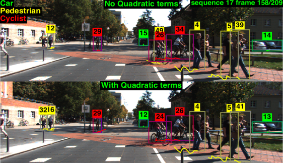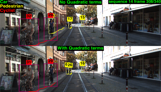
Multi-target tracking is an active area of research in computer vision, driven in part by the desire to build autonomous systems that can navigate in crowded urban environments (see e.g., Geiger et al (2013)). Thanks to advances of object detector performance in single, static images, “tracking-by-detection” approaches that build tracks on top of a collection of candidate object detections have shown great promise. Tracking-by-detection avoids some problems such as drift and is often able to recover from extended periods of occlusion since it is “self-initializing”. Finding an optimal set of detections corresponding to each track can often be formulated as a discrete optimization problem of selecting a set of low-cost paths through a graph of candidate detections for which there are efficient combinatorial algorithms (such as min-cost matching or min-cost network-flow) that yield globally optimal solutions (Zhang et al (2008); Pirsiavash et al (2011)).

Tracking by detection differs from traditional generative formulations of multi-target tracking, which draw a distinction between the problem of estimating a latent continuous trajectory for each object from the discrete per-frame data association problem of assigning observations (e.g., detections) to underlying tracks. Such methods (e.g., Milan et al (2012, 2013); Wu et al (2012)) allow for explicitly specifying an intuitive model of trajectory smoothness but face a difficult joint inference problem over both continuous and discrete variables which can seldom be solved with any guarantee of optimality.

In tracking by detection, trajectories are implicitly defined by the selected group of detections associated with a track. For example, a track may skip over some frames entirely due to occlusions or missing detections. The transition cost of utilizing a given edge between detections in successive frames thus could be interpreted as some approximation of the marginal likelihood associated with integrating over a set of underlying continuous trajectories associated with the corresponding pair of detections. This viewpoint immediately raises difficulties, both in (1) encoding strong trajectory models with only pairwise potentials and (2) identifying the parameters of these potentials from training data.

The contribution of this paper is in demonstrating that carefully optimizing the parameters of relatively simple combinatorial tracking-by-detection models can yield state-of-the-art performance on difficult tracking benchmarks. Building on our preliminary work (Wang and Fowlkes (2015)), we introduce a simple multi-target, multi-category tracking model that extends min-cost flow with quadratic interactions between tracks in order to capture contextual interactions within a frame. To perform inference, we propose a family of greedy-dynamic programming algorithms that produce high-quality solutions on par with linear programming relaxations of the quadratic tracking objective while being substantially faster than a general purpose LP solver.

For learning, we use a structured prediction SVM (Taskar et al (2003)) to optimize the complete set of tracking parameters from labeled training data. Structured prediction has been applied in tracking to learning inter-frame affinity metrics (Kim et al (2013)) and association (Lou and Hamprecht (2011)) as well as a variety of other learning tasks such as fitting CRF parameters for segmentation (Szummer et al (2008)) and word alignment for machine translation (Lacoste-Julien et al (2006)).

The structure of the remainder of the paper is as follows. We provide a brief overview of recent related work in Section 2 and review the now classical network-flow model for multi-target tracking in Section 3 before introducing our quadratic interaction model. In Section 4 we describe inference algorithms for network-flow models with quadratic interactions, namely, a standard LP-relaxation and rounding method, and a family of novel greedy dynamic programming algorithms that can handle quadratic interactions. In Section 5 we describe the features we used for learning tracking potentials in network-flow model with quadratic costs. In Section 6 we describe an approach to joint learning of model parameters in order to maximize tracking performance on a training data set using techniques for structured prediction. We conclude with experimental results (Section 7) which demonstrate that with properly learned parameters, even the basic network-flow yields better results than many state-of-the-art methods on challenging MOT and KITTI benchmarks. We also find that quadratic terms offer further improvements in performance for multi-category object tracking.

2 Related Work

Multi-target tracking problems have been tackled in a number of different ways. One approach is to first group detections into candidate tracklets and then perform scoring and association of these tracklets (Yang and Nevatia (2012); Brendel et al (2011); Wang et al (2014)). Compared to individual detections, tracklets allow for evaluating much richer trajectory and appearance models while maintaining some benefits of purely combinatorial grouping. However since the problem is at least two-layered (tracklet-generation and tracklet-association), these models are difficult to reason about mathematically and typically lack guarantees of optimality. Furthermore, tracklet-generation can only be done offline (or with substantial latency) and thus approaches that rely on tracklets are inherently limited in circumstances where online tracking is desired.

An alternative to tracklets is to attempt to include higher-order constraints directly in a combinatorial framework (Butt and Collins (2013); Chari et al (2015)). Such methods often operate directly over raw detections, either in an online or offline-fashion. Offline formulations benefit from having a single well-defined objective function or likelihood, and thus can give either globally optimal solution (Zhang et al (2008)), or provide approximate solution with a certificate of (sub)optimality (Chari et al (2015)). Tang et al (2015) propose a subgraph multi-cut approach which differs from traditional “path-finding” algorithms such as Zhang et al (2008), Pirsiavash et al (2011) and Butt and Collins (2013). Although designed to work directly on raw detections, in practice Tang et al (2015) use tracklets to reduce the dimension of the inference problem. Such is the trade-off between finding globally optimal solutions and using rich tracking features.

Milan et al (2012) attempt to solve both data association and trajectory smoothing problem simultaneously, which results in a problem with varying dimensionality and difficult approximate inference. Brau et al (2013) avoid this varying dimensionality problem by integrating out trajectory-related variables and using Markov Chain Monte Carlo sampling to estimate the marginal likelihoods for data association and trajectory estimation. Segal and Reid (2013) propose yet another way to avoid varying dimensionality: instead of explicitly enumerating number of tracks, they assign a latent variable for each real detection/track and conduct data association on these latent variables.

Online tracking algorithms take advantage of previously identified track associations to build rich feature models over past trajectories that facilitate data association at the current frame. The capability to perform streaming data association on incoming video-frames without seeing the entire video is a desirable property for real-time applications such as autonomous driving. However, when the whole video is available, online tracking may make errors that are avoidable in offline algorithms that access future frames to resolve ambiguities.  Kim et al (2015) revisit the legacy Multiple Hypothesis Tracking method and introduc a novel online recursive appearance filter. Choi (2015) proposes a novel flow-descriptor designed specifically for multi-target tracking and introduces a delay period to allow correction of possible errors made in previous frames (thus the name “near online”), which yields state-of-the-art accuracy.  Solera et al (2015) use the relatively simple Hungarian Matching with the novel extension to choose either “simple” or “complex” features depending on the difficulty of the inference problem at each frame.

For any multi-target tracking approach, there are a large number of associated model parameters which must be accurately tuned to achieve high performance. This is particularly true for (undirected) combinatorial models based on, e.g., network-flow, where parameters have often been set empirically by hand or learned using piecewise training. Solera et al (2015) and Dehghan et al (2015) both use structured SVM to learn parameters of their online data association models. Choi and Savarese (2012) use structured SVM to learn parameters for offline multi-target tracking with quadratic interactions for the purpose of activity recognition. Our work differs in that it focuses on generic activity-independent tracking and global end-to-end formulation of the learning problem. In particular, we develop a novel loss function that penalizes false transition and id-errors based on the MOTA (Bernardin and Stiefelhagen (2008)) tracking score.

Finally, recent work has also pursued detectors which are specifically optimized for tracking scenarios.  Tang et al (2013) propose to learn multi-person detector by using hard-negatives acquired from a tracker’s output, in order to let the detector to solve ambiguities that the tracker cannot handle. Dehghan et al (2015) propose to use a target identity-aware network-flow model to process videos in batches of frames, and learn people detectors for each individual person in an online fashion.

3 Models for Multi-target Data Association

We begin by formulating multi-target tracking and data association as a min-cost network flow problem equivalent to that of Zhang et al (2008), where individual tracks are described by a first-order Markov Model whose state space is a set of spatial-temporal locations in a video. This framework incorporates a state transition likelihood that generates dynamics associated with a pair of successive detections along a track, and an observation likelihood that generates appearance features for objects and background in a given frame. In the subsequent section we augment this model with quadratic interactions between pairs of tracks.

3.1 Tracking by Min-cost Flow

For a given video sequence, we consider a discrete set of candidate object detection sites $V$ where each candidate site $x=(l,\sigma,t)\in V$ is a tuple described by its location $l$, scale $\sigma$ and discrete time $t$. We write $\Phi=\{\phi_{a}(x)|x\in V\}$ for the appearance features (image evidence) extracted at each corresponding spatial-temporal location in a video. A single tracked object consists of an ordered set of detection sites, $T=\{x_{1},...,x_{n}\}$, where the times of successive sites are strictly increasing.

We model the whole video by a collection of tracks $\mathcal{T}=\{T_{1},...,T_{k}\}$, each of which independently generates foreground object appearances at the corresponding sites according to distribution $p_{fg}(\phi_{a})$ while the remaining site appearances are generated by a background distribution $p_{bg}(\phi_{a})$. Each site can only belong to at most a single track which we express by the constraint $\mathcal{T}\in\Omega$. We use $\mathcal{B}=V\setminus\bigcup\limits_{T\in\mathcal{T}}T$ to denote the sites which are unclaimed by any track. Our task is to infer a collection of tracks that maximize the posterior probability $P(\mathcal{T}|\Phi)$. Assuming that tracks behave independently of each other and follow a first-order Markov model, we can write an expression for MAP inference:

$$\mathcal{T}^{*} =\underset{\mathcal{T}\in\Omega}{\operatorname{argmax}}\;P(\Phi|\mathcal{T})\times P(\mathcal{T})$$

$$\begin{split}&=\underset{\mathcal{T}\in\Omega}{\operatorname{argmax}}\;\prod_{T\in\mathcal{T}}\big{[}\prod_{x\in T}p_{fg}(\phi_{a}(x))\big{]}\prod_{x\in\mathcal{B}}p_{bg}(\phi_{a}(x))\times\\ &\quad\quad\quad\quad\prod_{T\in\mathcal{T}}\big{[}p_{s}(x_{1})\prod_{i=1}^{n-1}p_{t}(x_{i+1}|x_{i})p_{e}(x_{n})\big{]}\end{split}$$ (1)

where $p_{s}$, $p_{e}$ and $p_{t}$ represent the likelihoods for tracks starting, ending and transitioning between given sites. Dividing through $\prod_{x\in V}p_{bg}(\phi_{a}(x))$ yields an equivalent problem that depends only on the appearance features at active track locations:

$$\begin{split}\mathcal{T}^{*}&=\underset{\mathcal{T}\in\Omega}{\operatorname{argmax}}\prod_{T\in\mathcal{T}}\big{[}\prod_{x\in T}l(\phi_{a}(x))\big{]}\times\\ &\quad\quad\prod_{T\in\mathcal{T}}\big{[}p_{s}(x_{1})\prod_{i=1}^{n-1}p_{t}(x_{i+1}|x_{i})p_{e}(x_{n})\big{]}\end{split}$$ (2)

where

$$l(\phi_{a}(x))=\frac{p_{fg}(\phi_{a}(x))}{p_{bg}(\phi_{a}(x))}$$

is the appearance likelihood ratio that a specific location $x$ corresponds to the object tracked.

The set of optimal (most probable) tracks under this model can be found by solving an integer linear program (ILP) over flow variables $\mathbf{f}$ that indicate which detections are active in each frame $\{f_{i}\}$ and which pairs of detections are associated between frames $\{f_{ij}\}$. Figure 2 shows a graphical representation where an individual object track corresponds to a directed st-path traversing edges that encode start, detection, transition and end costs. By taking a negative log of the MAP objective, this equivalent formulation can be written as:

$$\underset{\mathbf{f}}{\operatorname{min}} \ \sum_{i\in V}c_{i}^{s}f_{i}^{s}+\sum_{ij\in E}c_{ij}f_{ij}+\sum_{i\in V}c_{i}f_{i}+\sum_{i\in V}c_{i}^{t}f_{i}^{t}$$ (3)

s.t. $$\quad f_{i}^{s}+\sum_{j}f_{ji}=f_{i}=f_{i}^{t}+\sum_{j}f_{ij}$$ (4)

$$f_{i}^{s},f_{i}^{t},f_{i},f_{ij}\in\{0,1\}$$ (5)

where $E$ is the set of valid transitions between sites in successive frames and the costs are given by:

$$\begin{split}c_{i}=-\log\frac{p_{fg}(\phi_{a}(x_{i}))}{p_{bg}(\phi_{a}(x_{i}))}&,\quad c_{ij}=-\log p_{t}(x_{j}|x_{i}),\\ c_{i}^{s}=-\log p_{s}(x_{i})&,\quad c_{i}^{t}=-\log p_{e}(x_{i})\end{split}$$ (6)

and the integrality constraint on $\mathbf{f}$ enforces the requirement that each site belongs to at most a single track.

This ILP is a well studied problem known as minimum-cost network flow (Ahuja et al (1993)) with unit capacity edges. In particular, the flow constraints satisfy the total unimodularity property and thus an integral solution can be found by LP relaxation or via efficient specialized solvers such as network simplex, successive shortest path and push-relabel with bisectional search (Zhang et al (2008)).

(a) network-flow model

(b) pairwise cost

Figure 2: Graphical representation of network flow model and its extension with pairwise costs. (a) Basic network-flow model for multi-target tracking, as described by Zhang et al (2008). A pair of nodes (connected by red edge) represent a detection, blue edges represent possible transitions between detections and track birth/death events are modeled by black edges. Costs $c_{i}$ in Eq. 3 are for red edges, $c_{ij}$ are for blue edges, $c_{i}^{t}$ and $c_{i}^{s}$ are for black edges. (b) Network-flow model extended with pairwise cost. A green node represents a detection site while an undirected edge between green nodes encodes the pairwise cost for choosing both detection sites as part of the solution. To simplify our description, in later text we will refer to a green node (a red edge and the two nodes associated with it) as a “detection node”. The set $V$ consists of all detection nodes in the graph, whereas the set $E$ consists of all transition edges in the graph.

3.2 Track Interdependence

The aforementioned model assumes tracks are independent of each other, which is not always true in practice. In order to allow interactions between multiple objects, we add a pairwise cost term denoted $q_{ij}$ for jointly activating a pair of flows $f_{i}$ and $f_{j}$ corresponding to detections at sites $x_{i}=(l_{i},\sigma_{i},t_{i})$ and $x_{j}=(l_{j},\sigma_{j},t_{j})$. Adding this term to Eq. 3 yields an Integer Quadratic Program (IQP):

$$\begin{split}\underset{\mathbf{f}}{\operatorname{min}}&\ \sum_{i\in V}c_{i}^{s}f_{i}^{s}+\sum_{ij\in E}c_{ij}f_{ij}+\sum_{i\in V}c_{i}f_{i}+\sum_{i\in V}c_{i}^{t}f_{i}^{t}\\ &+\sum_{ij\in EC}q_{ij}f_{i}f_{j}\end{split}$$ (7)

s.t. $$\quad f_{i}^{s}+\sum_{j}f_{ji}=f_{i}=f_{i}^{t}+\sum_{j}f_{ij}$$

$$\quad f_{i}^{s},f_{i}^{t},f_{i},f_{ij}\in\{0,1\}$$

In our experiments, we only consider pairwise interactions between pairs of sites in the same video frame which we denote by $EC=\{ij:t_{i}=t_{j}\}$. One could easily extend such formulation to include transition-transition interactions to model high order dynamics.

Unlike min-cost flow (Eq. 3), finding the global minimum of the IQP problem (Eq. 7) is NP-hard (Zaied and Shawky (2014)) due to the quadratic terms in the objective. In the next section we discuss two different approximations for finding high-quality solutions $\mathbf{f}$. In Section 6 we describe how the costs $\mathbf{c}$ and $\mathbf{q}$ can be learned from data.

4 Inference

We evaluate two different schemes for finding high-quality approximate solutions to the quadratic tracking objective. The first is a standard approach of introducing auxiliary variables and relaxing the integrality constraints to yield a linear program (LP) that lower-bounds the original objective. We also consider a family of greedy approximation algorithms based on successive rounds of dynamic programming that also yields good solutions while avoiding the expense of solving a large scale LP. The resulting tracks (encoded by the optimal flows $\mathbf{f}$) are used for both test-time track prediction as well as for optimizing parameters during learning (see Section 6).

4.1 LP Relaxation and Rounding

If we relax the integer constraints and deform the costs as necessary to make the objective convex, then the global optimum of Eq. 7 can be found in polynomial time. For example, one could apply Frank-Wolfe algorithm to optimize the relaxed, convexified QP while simultaneously keeping track of good integer solutions (Joulin et al (2014)). However, for real-world tracking over long videos, the relaxed QP is still quite expensive to solve. Instead we follow the approach proposed by Chari et al (2015), reformulating the IQP as an equivalent ILP problem by replacing the quadratic terms $f_{i}f_{j}$ with a set of auxiliary variables $u_{ij}$:

$$\begin{split}\underset{\mathbf{f}}{\operatorname{min}}&\ \sum_{i\in V}c_{i}^{s}f_{i}^{s}+\sum_{ij\in E}c_{ij}f_{ij}+\sum_{i\in V}c_{i}f_{i}+\sum_{i\in V}c_{i}^{t}f_{i}^{t}\\ &+\sum_{ij\in EC}q_{ij}u_{ij}\end{split}$$ (8)

$$\begin{split}\text{s.t.}&\quad f_{i}^{s}+\sum_{j}f_{ji}=f_{i}=f_{i}^{t}+\sum_{j}f_{ij}\\ &\quad f_{i}^{s},f_{i}^{t},f_{i},f_{ij}\in\{0,1\}\\ &\quad u_{ij}\leq f_{i},u_{ij}\leq f_{j}\quad f_{i}+f_{j}\leq u_{ij}+1\end{split}$$

The new constraint sets enforce $u_{ij}$ to be $1$ only when $f_{i}$ and $f_{j}$ are both $1$. By relaxing the integrality constraints, the program in Eq. 8 can be solved efficiently via large scale LP solvers such as CPLEX or MOSEK.

During test time we would like to predict a discrete set of tracks. This requires rounding the solution of the relaxed LP to some solution that satisfies not only integer constraints but also flow constraints.  Chari et al (2015) proposed two rounding heuristics: a Euclidean rounding scheme that minimizes $\|\mathbf{f}-\widehat{\mathbf{f}}\|^{2}$ where $\widehat{\mathbf{f}}$ is the non-integral solution given by the LP relaxation. When $\mathbf{f}$ is constrained to be binary, this objective simplifies to a linear function $(\mathbf{1}-2\widehat{\mathbf{f}})^{T}\mathbf{f}+\|\widehat{\mathbf{f}}\|^{2}$, which can be optimized using a standard linear min-cost flow solver. Alternately, one can use a linear under-estimator of the objective in Eq. 7, similar to the Frank-Wolfe algorithm:

$$\begin{split}&\underset{\mathbf{f}}{\operatorname{min}}\sum_{i\in V}c_{i}^{s}f_{i}^{s}+\sum_{ij\in E}c_{ij}f_{ij}+\sum_{i\in V}c_{i}^{t}f_{i}^{t}\\ &\quad\quad+\sum_{i\in V}(c_{i}+\sum_{ij\in EC}q_{ij}\widehat{u}_{ij}+\sum_{ji\in EC}q_{ji}\widehat{u}_{ji})f_{i}\end{split}$$ (9)

Both of these rounding heuristics involve optimizing a new linear objective function subject to the original integer and flow constraints and thus can be solved as an ordinary min-cost network flow problem. In our experiments we execute both rounding heuristics and choose the solution with lower cost under the original quadratic objective.

4.2 Greedy Dynamic Programming

As an alternative to the LP relaxation, we describe a family of greedy algorithms inspired by the combination of dynamic programming (DP) proposed by  Pirsiavash et al (2011) for approximately solving min-cost flow and the greedy forward selection used for modeling contextual object interactions by Desai et al (2009). Our general strategy is to sequentially push units of flow through the tracking graph, updating the edge costs at each step to capture the expected contribution of quadratic interactions.

4.2.1 Successive Shortest Paths

We start by briefly describing the successive shortest path (SSP) algorithm which solves for the min-cost flow with the standard linear objective and refer the reader to Ahuja et al (1993) for a comprehensive discussion. Consider the example tracking graph shown in Figure 2. SSP finds the global optimum of Eq. 3 by repeatedly searching for shortest st-path in a so-called residual graph. In our model where all edges have unit capacity, the residual graph $G_{r}(\mathbf{f})$ associated with flow $\mathbf{f}$ is given by reversing the orientation of every directed edge used by the solution $\mathbf{f}$ and negating their associated costs.

Starting from an empty flow $\mathbf{f}=0$, SSP simply iterates two steps,

1. Find the minimum cost st-path in the residual graph $G_{r}(\mathbf{f})$.

2. If the cost of the path is negative, push a unit flow along the path and update $\mathbf{f}$.

until no negative cost path can be found.

We note that the first iteration of SSP looks like a single-target data association problem. In particular, one can utilize a simple dynamic program that makes a single sweep over the graph nodes ordered by time to find the minimum cost (shortest) path. However, the residual graph in subsequent iterations contains negative weight edges and is no longer acyclic, hence requiring the use of a more general and computationally expensive shortest path algorithm such as Bellman-Ford.

Here we consider fast approximations to the full shortest path problem based on carrying out multiple temporally-ordered sweeps of the graph. This “K-Pass Dynamic Program” approach introduced by Pirsiavash et al (2011) can be viewed as a variant of Bellman-Ford that only considers a subset of possible shortest paths using a problem-specific schedule for performing edge relaxations. This approximate approach has been shown to provide solutions which are nearly as good as the full shortest path computation and provides a natural way to incorporate quadratic cost terms.

4.2.2 One-pass Dynamic Programming

Assume the detection nodes are sorted in time. We denote $cost(i)$ as the cost of the shortest path from source node to node $i$, $link(i)$ as $i$’s predecessor in this shortest path, and $birth\_node(i)$ as the first detection node in this shortest path. We initialize $cost(i)=c_{i}+c_{i}^{s}$, $link(i)=\emptyset$, and $birth\_node(i)=i$ for all $i\in V$.

To find the shortest path on the initial DAG $G$, we can sweep from first frame to last frame, computing $cost(i)$ as:

$$cost(i)=c_{i}+\underset{j:ij\in E}{\operatorname{min}}\;\left\{c_{i}^{s},\;c_{ij}+cost(j)\right\}$$ (10)

and store the argmin in $birth\_node(i)$ or $link(i)$ accordingly.

After sweeping through all frames, we find a node $i$ such that $cost(i)+c_{i}^{t}$ is minimum and reconstruct the corresponding shortest path (which terminates at $i$ and has cost $cost(i)+c_{i}^{t}$) by backtracking cached $link$ variables. After the shortest path is identified, we remove all nodes and edges in this path from $G$; the resulting graph $G^{\prime}$ will still be a DAG. Without quadratic terms we can just repeat this procedure until we cannot find any path that has a negative cost. This can be viewed as a greedy version of SSP that does not change paths once they have been added to the solution.

Quadratic cost updates

The sequential greedy nature of one-pass dynamic programming is well suited to incorporating estimates of the quadratic cost terms in Eq. 7 by performing an additional contextual update step after each round of dynamic programming. The complete algorithm is outlined in Algorithm 1. After each new track is instanced, the edge costs in the associated flow graph used for finding tracks in subsequent iterations are updated to include the quadratic penalties or boosts incurred by the newly instanced track. As was the case with the LP+rounding scheme described in Section 4.1, Algorithm 1 does not guarantee an optimal solution. However, as we show in the experiments, it performs well in practice.

Algorithm 1 One-pass DP with Quadratic Cost Update

1:Input: A Directed-Acyclic-Graph $G$ with edge weights $c_{i},c_{ij}$

2:initialize $\mathcal{T}\leftarrow\emptyset$

3:repeat

4:     Find shortest st-path $\mathbf{p}$ on $G$ via dynamic programming

5:     $track\_cost=cost(\mathbf{p})$

6:     if $track\_cost<0$ then

7:         for all locations $x_{i}$ in $\mathbf{p}$ do

8:              $c_{j}=c_{j}+q_{ij}+q_{ji}$ for all $ij\in EC$

9:              $c_{i}=+\infty$

10:         end for

11:         $\mathcal{T}\leftarrow\mathcal{T}\cup\mathbf{p}$

12:     end if

13:until $track\_cost\geq 0$

14:Output: track collection $\mathcal{T}$

4.2.3 Two-pass Dynamic Programming

Unlike a general shortest path algorithm such as Bellman-Ford, one-pass dynamic programming can only find shortest paths consisting of forward going edges. As proposed by Pirsiavash et al (2011), one can improve this approximation by carrying out multiple passes of DP that run forward and backward in time to find paths in the residual graph $G_{r}(\mathbf{f})$ that reverse temporal direction one or more times. First we describe the details of 2-pass dynamic programming without quadratic contextual updates.

Let $V_{f}$ denote the set of forward edges in the current residual graph, i.e., detection and transition variables in $\mathbf{f}$ that equal 0, and $V_{b}$ as the set of backward edges in current residual graph, i.e., variables in $\mathbf{f}$ that equal 1. The 2-pass DP algorithm proceeds as follows:

1. Perform a pass of forward DP (from first frame to last frame) on all nodes. When computing $cost$ of a specific node, simply ignore all its predecessors that belong to $V_{b}$.

2. Set $cost_{en}(i)=cost(i)-c_{i}$ for all $i\in V_{b}$ and perform one pass of backward DP (from last frame to first frame) on $V_{b}$. Update $cost(i)$ and $cost_{en}(i)$ for $i\in V_{b}$ at each step,

   $$cost(i)=cost_{en}(j)-c_{ij}$$ (11)

   $$cost_{en}(i)={\operatorname{min}}\;(cost_{en}(i),cost(i)-c_{i})$$ (12)

   where $j$ is $i$’s backward predecessor and $c_{ij}$ is from the original graph. Set $cost(i)=+\infty$ for any backward detection $i$ that has no backward transition edge coming to it (i.e., the last node of each instanced track).

3. Perform a second pass of forward DP on $i\in V_{f}$. To avoid running into cyclic path, we need to backtrack shortest paths for all $j\in N(i)$, where $N(i)$ is all neighboring nodes that are connected to $i$ via a forward edge. In practice we only need to check $j\in N(i)$ such that $j$ and $i$ share the same birth node, as they cannot form a cyclic path otherwise. Furthermore, one can keep a cache of shortest path so far for each node, reducing the backtrack to a constant $O(1)$ operation.

4. Find node $i$ with minimum $cost(i)+c_{i}^{t}$, the (approximate) shortest path is then $path(i)$.

5. Update solution $\mathbf{f}$ by setting all forward variables along $path(i)$ to 1 and all backward variables along $path(i)$ to 0.

It is straightforward to see that during the first iteration, 1-pass DP and 2-pass DP behave identically. Since we enforce the path found by 2-pass DP never goes into a source node or out of a sink node, each iteration generates exactly one more track (either by splitting a previously found track into two or by instancing an entirely new track). Therefore the algorithm will terminate after at most $|V|$ iterations.

Quadratic cost updates

The path found by 2-pass DP may contain both forward and backward detection edges which correspond to newly instanced and removed detections respectively. When we augment the flow with this new path, we also update the (unary) cost of other nodes by adding or subtracting the pairwise cost imposed by turning on or off selected nodes on the path. The entire procedure is described as Algorithm 2 and illustrated in Figure 3.

Algorithm 2 Two-pass DP with Quadratic Cost Update

1:Input: A Directed-Acyclic-Graph $G$ with node and edge weights $c_{i},c_{ij}$

2:initialize $\mathbf{f}=\mathbf{0}$

3:repeat

4:     Find a shortest st-path $\mathbf{p}$ in $G_{r}(\mathbf{f})$ using 2-pass DP

5:     $track\_cost=cost(\mathbf{p})$

6:     if $track\_cost<0$ then

7:         for all locations $x_{i}\in\mathbf{p}$ do

8:              if $f_{i}=0$ then

9:                  $c_{j}=c_{j}+q_{ij}+q_{ji},\forall ij\in EC$

10:              else

11:                  $c_{j}=c_{j}-q_{ij}-q_{ji},\forall ij\in EC$

12:              end if

13:         end for

14:         $\mathbf{f}(\mathbf{p})=\mathbf{1}-\mathbf{f}(\mathbf{p})$

15:     end if

16:until $track\_cost\geq 0$

17:Output: Solution $\mathbf{f}$

Notice that to simplify our notation, we construct temporary residual graph at the beginning of each iteration based on the current costs. In practice, we instead update edge costs and directions on the original graph at the end of each iteration. When operating in place on the residual graph, the signs of the cost updates are reversed when updating costs of reversed detection edges (i.e., when turning off a detection, we subtract pairwise costs from forward detection edges but add pairwise costs to reversed detection edges).

(a)

(b)

(c)

(d)

(e)

Figure 3: An illustration for 2-pass DP with quadratic interactions. (a) the initial DAG graph, a pair of nodes indicate a candidate detection; (b) first iteration of the algorithm, red edges indicates the shortest path found in this iteration; (c) we reverse all the edges along the shortest path (green edges), and add the pairwise cost imposed by this path to other candidates detections at each time point (red node pairs). (d) In the second iteration of the algorithm, red edges and blue edges indicate the new shortest path which happens to traverse three of the reversed edges (shown in blue); (e) we again reverse all the edges along the shortest path yielding two instanced st-tracks (green edges). We again update pairwise cost: blue node pair indicates we subtract the pairwise cost imposed by “turning off” a candidate, red pair indicates adding in pairwise cost of newly instanced candidates, and the blue-red pair indicates we first add the pairwise cost by newly instanced candidates, then subtract the pairwise cost by newly uninstanced candidates. Additions and subtractions are done to the non-negated edge costs and then negated if necessary.

4.2.4 Caching DP messages

Similar to the speed-up techniques employed by Pirsiavash et al (2011), DP algorithms with contextual updates only need to re-evaluate a subset of all detection nodes in each round of shortest path computation. For one-pass DP, we need to re-evaluate detection nodes who have the same birth node as either newly found shortest path or suppressed nodes, i.e., nodes whose cost has been increased due to most recent contextual update. Then, we also need to count the effect of boosted nodes whose cost has been decreased due to most recent contextual update; this is done by first setting all boosted nodes to be active, re-evaluating their successors and propagating this activity to nodes whose $link$ points back to the active nodes. The caching scheme is similar for two-pass DP, only difference being that we have to conduct two forward passes and one backward pass, thus we need to maintain separate caches for each pass.

4.2.5 Time Complexity Analysis

For the basic network-flow problem in Eq. 3 with $n$ total variables in $\mathbf{f}$ and $k$ detections, exact successive shortest path using Dijkstra’s algorithm has a worst-case performance of $O(n\log k)$ operations per path and terminates after adding fewer than $k$ paths yielding $O(nk\log k)$ worst-cast performance. The family of DP algorithms introduced by Pirsiavash et al (2011) takes $O(n)$ to find a single track and thus has worst-case performance of $O(kn)$ for basic network-flow problem.

For solving the linear program in Eq.  8, a general solver such as simplex has average run times of $O(n^{3})$, where $n$ is the total number of variables (unary and pairwise). For a video with $k$ total detections, our one-pass DP algorithm takes $O(n)$ to find a single track, achieving a worst case $O(kn)$ time complexity. Notice that $k$ is often much smaller than $n$; in fact, for short sequences $n$ often grows quadratically with $k$. The same $O(kn)$ worst-case time complexity applies for 2-pass DP or any number of constant passes because the complexity of every iteration of multi-pass DP still scales linearly with $n$.

5 Features for Scoring Tracks

In order to learn the tracking potentials ($\mathbf{c}$ and $\mathbf{q}$) we parameterize the flow cost objective by a vector of weights $\mathbf{w}$ and a set of features $\Psi(X,\mathbf{f})$ that depend on features extracted from the video, the spatio-temporal relations between candidate detections, and which tracks are instanced. With this linear parameterization we write the cost of a given flow as $C(\mathbf{f})=\mathbf{w}^{T}\Psi(X,\mathbf{f})$ where the vector components of the weight and feature vector are given by:

$$\mathbf{w}=\begin{bmatrix}w_{S}\\ w_{t}\\ w_{s}\\ w_{a}\\ w_{E}\end{bmatrix}\indent\Psi(X,\mathbf{f})=\begin{bmatrix}\sum_{i}\phi_{S}(x_{i}^{s})f_{i}^{s}\\ \sum_{ij\in E}\psi_{t}(x_{i},x_{j})f_{ij}\\ \sum_{ij\in EC}\psi_{s}(x_{i},x_{j})f_{i}f_{j}\\ \sum_{i}\phi_{a}(x_{i})f_{i}\\ \sum_{i}\phi_{E}(x_{i}^{t})f_{i}^{t}\end{bmatrix}$$ (13)

Here $w_{a}$ represents local appearance template for the tracked objects of interest, $w_{t}$ represents weights for transition features, $w_{s}$ represents weights for pairwise interactions, $w_{S}$ and $w_{E}$ represents weights associated with track births and deaths. $\Psi(X,\mathbf{f})$ are corresponding features. Given the wegiht vector $\mathbf{w}$, we extract features on each node $i$, including detections $\phi_{a}(x_{i})$ and track birth/deaths $\phi_{S}(x_{i}^{s})$,$\phi_{E}(x_{i}^{t})$, along with features on each edge $ij\in E$ and $ij\in EC$, including transitions $\psi_{t}(x_{i},x_{j})$ and pairwise interactions $\psi_{s}(x_{i},x_{j})$. Then we multiply corresponding weight vectors and features on each edge. In this way we can obtain costs of each node/edge in the network and conduct standard inference as described in Section 4. We describe each type of features as below:

Local appearance and birth/death model

We make use of off-the-shelf detectors (Dollár et al (2014); Felzenszwalb et al (2010); Wang et al (2013)) to capture local appearance. Our local appearance feature thus consists of the detector score along with a constant 1 to allow for a variable bias. In applications with static cameras it can be useful to learn a spatially varying bias to model where tracks are likely to appear or disappear. However, most videos in our experiments are captured from moving platforms, we thus use a single constant value 1 for the birth and death features.

Transition model

We connect a candidate $x_{i}$ at time $t_{i}$ with another candidate $x_{j}$ at a later time $t_{i}+n$, only if the overlap ratio between $x_{i}$’s window and $x_{j}$’s window exceeds $0.3$. The overlap ratio is defined as two windows’ intersection over their union. We use this overlap ratio to compute a binary overlap feature associated with each transition link which is 1 if the overlap ratio is lower than 0.5, and 0 otherwise. In order to handle occlusion, we allow up to 8 frames(10 on PETS+TUD-Stadtmitte) gap between the two detection sites of a transition edge. We jointly encode the overlap and frame gap with a single 16 dimensional (20 on PETS+TUD-Stadtmitte) binary feature for each transition link.

Pairwise interactions

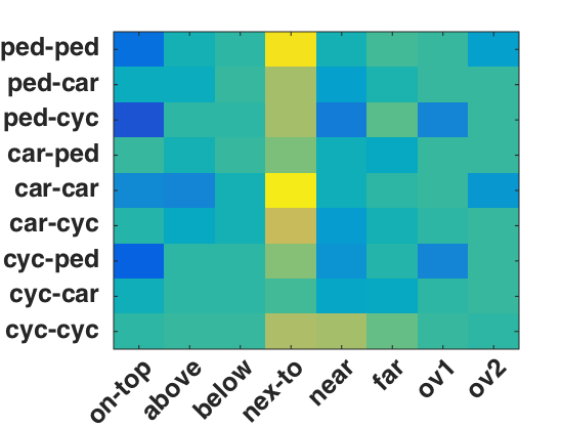
The weight vector $w_{s}$ encodes valid geometric configurations of two tracked objects in a frame. $\psi_{s}(x_{i},x_{j})$ is a discretized spatial-context feature that bins relative location of detection window at location $x_{i}$ and window at location $x_{j}$ into one of the $D$ relations including on top of, above, below, next-to, near, far and overlap (similar to the spatial context by Desai et al (2009)). To mimic the temporal NMS described by Pirsiavash et al (2011) we add one additional relation, strict overlap, which is set to 1 if the ratio of the intersection area of two boxes over the area of the first box is greater than 0.9. If we assume that there are $K$ classes of objects in the video, then $w_{s}$ is a $DK^{2}$ vector, $w_{s}=[w_{s11}^{T},w_{s12}^{T},...,w_{sij}^{T},...,w_{sKK}^{T}]^{T}$, in which $w_{sij}$ is a length of $D$ column vector that encodes valid geometric configurations of object of class $i$ w.r.t. object of class $j$. This allows the model to capture intra- and inter-class contextual relationships between tracks.

6 Learning

We formulate parameter learning of tracking models as a structured prediction problem. With some abuse of notation, assume we have $N$ labeled training videos $(X_{n},\mathbf{f}_{n})\in\mathcal{X}\times\mathcal{F}$ indexed by $n=1,...,N$. Given ground-truth tracks in training videos specified by flow variables $\mathbf{f}_{n}$, we discriminatively learn tracking model parameters $\mathbf{w}$ using a structured SVM with margin scaling:

$$\mathbf{w}^{*}=\underset{\mathbf{w},\xi_{n}\geq 0}{\operatorname{argmin}}\ \frac{1}{2}\|\mathbf{w}\|^{2}+C\sum_{n}\xi_{n}$$ (14)

s.t. $$\ \mathbf{w}^{T}\Psi(X_{n},\widehat{\mathbf{f}})-\mathbf{w}^{T}\Psi(X_{n},\mathbf{f}_{n})\geq L(\mathbf{f}_{n},\widehat{\mathbf{f}})-\xi_{n}\quad\forall n,\widehat{\mathbf{f}}$$

$\Psi(X_{n},\mathbf{f}_{n})$ are the features extracted from $n$th training video. $L(\mathbf{f}_{n},\widehat{\mathbf{f}})$ is a loss function that penalizes any difference between the inferred label $\widehat{\mathbf{f}}$ and the ground truth label $\mathbf{f}_{n}$ and which satisfies $L(\mathbf{f},\mathbf{f})=0$. The constraint on the slack variables $\xi_{n}$ ensure that we pay a penalty for any training videos in which the cost of the flow associated with ground-truth tracks under model $\mathbf{w}$ is higher than some other incorrect flow $\widehat{\mathbf{f}}$.

6.1 Cutting Plane Optimization

We optimize the structured SVM objective in Eq. 14 using a standard cutting-plane method (Joachims et al (2009)) in which the exponential number of constraints (one for each possible flow $\widehat{\mathbf{f}}$) are approximated by a much smaller number of terms. Given a current estimate of $\mathbf{w}$ we find a “most violated constraint” for each training video:

$$\widehat{\mathbf{f}}_{n}^{*} =\underset{\widehat{\mathbf{f}}}{\operatorname{argmin}}\ \langle\mathbf{w},\Psi(X_{n},\widehat{\mathbf{f}})-\Psi(X_{n},\mathbf{f_{n}})\rangle-L(\mathbf{f_{n}},\widehat{\mathbf{f}})$$ (15)

We then add constraints for the flows $\{\widehat{\mathbf{f}}_{n}^{*}\}$ to the optimization problem and solve for an updated $\mathbf{w}$. This procedure is iterated until no additional constraints are added to the problem. In our implementation, at each iteration we add a single linear constraint which is a sum of violating constraints derived from individual videos in the dataset. This linear combination is also a valid cutting plane constraint (Desai et al (2009)) and yields faster overall convergence.

The key subroutine is finding the most-violated constraint for a given video which requires solving the loss-augmented inference problem Eq. 15. As long as the loss function $L(\mathbf{f},\widehat{\mathbf{f}})$ decomposes as a sum over flow variables then this problem has the same form as our test-time tracking inference problem, the only difference being that the cost of variables in $\mathbf{f}$ is augmented by their corresponding negative loss.

We note that this formulation allows for constraints corresponding to non-integral flows $\widehat{\mathbf{f}}$ so we can directly use the LP relaxation (Eq. 8) to generate violated constraints during training. Finley and Joachims (2008) point out that besides optimality guarantees, including non-integral constraints naturally pushes the SVM optimization towards model parameters that produce integer solutions even before rounding.

6.2 Tracking Loss Function

We find that a critical aspect for successful learning is to use a loss function that closely resembles major tracking performance criteria, such as Multiple Object Tracking Accuracy (MOTA). Metrics such as false positive, false negative, true positive, true negative and true/false birth/death can be easily incorporated using a standard Hamming loss on the flow vector. However, id switches and fragmentations are determined by looking at labels of two consecutive transition links simultaneously and hence cannot be optimized by our inference routine (which only considers pairwise relations between detections within a frame). Instead, we propose a decomposable loss for transition links that attempts to capture important aspects of MOTA by taking into account the length and localization of transition links rather than simply using a constant (Hamming) loss on mislabled links.

We define a weighted Hamming loss to measure distance between ground-truth tracks $\mathbf{f}$ and inferred tracks $\widehat{\mathbf{f}}$ that includes detections/birth/death, $f_{i}$, and transitions, $f_{ij}$. Let

$$L(\widehat{\mathbf{f}},\mathbf{f})=\sum_{i}l_{i}\left|f_{i}-\widehat{f_{i}}\right|+\sum_{ij}l_{ij}\left|f_{ij}-\widehat{f_{ij}}\right|$$

where $\mathbf{l}=\{l_{1},...,l_{i},...,l_{ij},...,l_{|\mathbf{f}|}\}$ is a vector indicating the penalty for differences between the estimated flow $\widehat{\mathbf{f}}$ and the ground-truth $\mathbf{f}$.

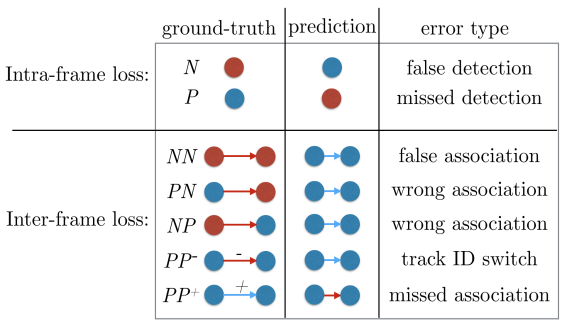
In order to describe our transition loss, let us first denote four types of transition links present in the tracking graph: $NN$ is the link from a false detection to another false detection, $PN$ is the link from a true detection to a false detection, $NP$ is the link from a false detection to a true detection, $PP^{+}$ is the link from a true detection to another true detection with the same identity, and $PP^{-}$ is the link from a true detection to another true detection with a different identity. These are depicted visually in Figure 4.

For all the transition links with a frame gap larger than 1, we interpolate detections between its start detection and end detection. The interpolated “virtual detections” are considered to be either true virtual detection or false virtual detection, depending on whether they overlap with a ground truth label or not. We define the losses for different types of transitions as:

1. $NN$ : $\;l_{ij}=$ ( # true virt. det. + # false virt. det.)

2. $PN$ : $\;l_{ij}=$ (# true virt. det. + # false virt. det. + 1)

3. $NP$ : $\;l_{ij}=$ (# true virt. det. + # false virt. det. + 1)

4. $PP^{-}$ : $\;l_{ij}=$ (# true virt. det. + # false virt. det. + 2)

5. $PP^{+}$ : $\;l_{ij}=$ (# true virt. det.)

Figure 4: Possible intra-frame and inter-frame errors a tracker could make which are penalized by our loss function. A blue node/edge indicates that corresponding flow variable is set to 1 in either ground-truth or tracker prediction. Similarly red node/edge indicates corresponding flow variable is set to 0.

6.3 Ground-truth flows from training data

Available training datasets specify ground-truth bounding boxes that need to be mapped onto ground-truth flow variables $\mathbf{f_{n}}$ for each video. To do this mapping, we first consider each frame separately. We take the highest scoring detection window that overlaps a ground truth label as true detection and assign it a track identity label which is the same as the ground truth label it overlaps. Next, for each track identity, we run a simplified version of the dynamic programming algorithm to find the path that claims the largest number of true detections. After we iterate through all id labels, any instanced graph edge will be a true detection/transition/birth/death while the remainder will be false.

An additional difficulty of training which arises on the KITTI tracking benchmark is special evaluation rules for ground truth labels such as small/truncated objects and vans for cars, sitting persons for pedestrians. This is resolved in our training procedure by removing all detection candidates that correspond to any of these “ambiguous” ground truth labels during training; in this way we avoid mining hard negatives from those labels. To speed up training on both MOT and KITTI dataset, we partition full-sized training sequences into 10-frame-long subsequences with a 5-frame overlap, and define losses on each subsequence separately.

7 Experimental results

Historically it has been challenging to make a meaningful empirical comparison among tracking performance results reported in the literature as the exact detection set, evaluation script, amount of training data and even ground-truth labels have varied greatly. As a result, there has been significant recent efforts to establish standard benchmarks for evaluating multi-target tracking algorithms. We focus our diagnostic analysis on the KITTI and MOT Challenge datasets as they have very clear train-test splits of data and the ground-truth labels for testing data are strictly “held out”, invisible to all competitors of the benchmark. To make our results easy to compare to other algorithms, we always use the base detections, ground-truth and evaluation scripts provided by the MOT and KITTI benchmark organizers when performing training, inference and diagnostics.

To aid comparison to older methods that have not been evaluted on MOT or KITTI, we also include results on PETS and the TUD-Stadtmitte sequence, based on what we believe to be the most popular public detection set, ground-truth and evaluation script. However, we note that for these videos the evaluation is less standardized and since ground-truth annotations have been used widely to tune models, there may be overfitting. We thus view these results as less informative than those on MOT and KITTI test benchmarks.

7.1 Datasets and Benchmarks

The Multiple Object Tracking Benchmark (Leal-Taixé et al (2015)) targets primarily pedestrian tracking. It contains sequences from widely-used multi-target tracking benchmarks such as TUD, ETH, PETS09, TownCentre and KITTI, augmented with several additional newly acquired sequences. The dataset is split into 11 training sequences and 11 testing sequences, with ground-truth labels of testing set held out on a private server.

The KITTI Tracking Benchmark (Geiger et al (2012)) involves multi-category tracking of cars, pedestrians and cyclists. It consists of 21 training sequences and 29 testing sequences which is much larger than the MOT dataset. Similar to the MOT benchmark, the ground-truth labels for testing set are also held out. Labels for the cyclist category are available on the training set but the benchmark server does not provide test-set benchmarks for cyclist. For both MOT and KITTI we allow up to 8 frames gap between two detection sites of a transition edge and determined the best regularization parameters via leave-one-video-out cross-validation on the training data.

Finally, in order to compare to previous related work such as Brau et al (2013) and Chari et al (2015), we use data provided by Milan et al (2013) consisting of 5 sequences from PETS09 dataset and the single TUD-Stadtmitte sequence. For this data, we report leave-one-video-out cross-validation results. We allow up to 10 frames gap between two detection sites of a transition edge in this setup and partition videos into 15-frame long sequences during training stage.

7.2 Evaluation Metrics

To evaluate the performance of each proposed tracker, we employ a standard battery of performance measure, which consists of the popular CLEAR MOT metric (Bernardin and Stiefelhagen (2008)) and the Mostly-Tracked/Mostly-Lost metric (Li et al (2009)):

• $MOTA(\uparrow)$: Multi-object Tracking Accuracy.

• $MOTP(\uparrow)$: Multi-object Tracking Precision.

• $MT(\uparrow)$: ratio of mostly-tracked ground-truth trajectories.

• $ML(\downarrow)$: ratio of mostly-lost ground-truth trajectories.

• $IDSW(\downarrow)$: total number of identity-switches.

• $FRAG(\downarrow)$: total number of times ground-truth trajectories are interrupted.

For measurements with $(\uparrow)$, higher scores indicate better performance; for measurements with $(\downarrow)$, lower scores indicate better performance.

MOT dataset

Benchmark on MOT test set
Method	MOTA	MOTP	MT	ML	IDSW	FRAG
Bae and Yoon (2014)	15.1%	70.5%	3.2%	55.8%	637	1716
Yoon et al (2015)	18.6%	69.6%	5.3%	53.3%	684	1282
Milan et al (2016)	19.6%	71.4%	5.1%	54.9%	521	819
Milan et al (2015)*	22.5%	71.7%	5.8%	63.9%	697	737
Leal-Taixé et al (2014)*	23.1%	70.9%	4.7%	52.0%	1018	1061
Xiang et al (2015)	30.3%	71.3%	13.0%	38.4%	680	1500
Kim et al (2015)	32.4%	71.8%	16.0%	43.8%	435	826
Choi (2015)	33.7%	71.9%	12.2%	44.0%	442	823
Ours(LP)	25.2%	71.7%	5.8%	53.0%	646	849

Cross-validation on MOT training set
Method	MOTA	MOTP	MT	ML	IDSW	FRAG
SSP	28.7%	72.9%	15.1%	50.5%	440	541
LP+Hamming	25.3%	72.4%	17.4%	46.5%	567	604
LP	28.5%	72.8%	15.1%	48.9%	440	563
DP1	27.6%	72.4%	15.5%	49.1%	492	626
DP2	28.5%	72.9%	15.5%	48.9%	476	592

Table 1: Benchmark and cross-validation results on MOT dataset. Gray background indicates the method uses target-specific appearance model, while asterisk(*) indicates method uses image-evidence, method with neither gray background nor asterisk can operate purely on bounding boxes without accessing images. We denote variants of our model as follows: 1) SSP is a model without any pairwise cost terms, learned and tested with successive shortest path algorithm. 2) LP are models with pairwise terms, learned with LP-Relaxation while tested with LP-Rounding. 3) DP1 and DP2 are models learned with LP-Relaxation and tested with 1-pass and 2-pass DP respectively. 4) LP+Hamming is the same as LP, except that models are learned using Hamming loss instead of the loss described in Section 6.

Benchmark on KITTI test set (as of 05/24/2016)
Benchmark on Car, DPM detections							Benchmark on Pedestrian, DPM detections
Method	MOTA	MOTP	MT	ML	IDSW	FRAG	Method	MOTA	MOTP	MT	ML	IDSW	FRAG
Geiger et al (2014)	54.2%	78.4%	13.9%	34.3%	31	535	Geiger et al (2014)	NA	NA	NA	NA	NA	NA
Milan et al (2014)	50.2%	77.1%	14.5%	34.0%	125	398	Milan et al (2014)	27.4%	68.5%	7.9%	52.9%	96	610
Yoon et al (2015)	51.5%	75.2%	15.2%	33.5%	51	382	Yoon et al (2015)	34.5%	68.1%	10.0%	47.4%	81	692
Choi (2015)	65.2%	78.2%	31.6%	27.9%	13	154	Choi (2015)	36.9%	67.8%	14.4%	42.6%	34	800
Ours(LP)	60.5%	76.9%	27.7%	23.8%	16	430	Ours(LP)	33.3%	67.4%	9.6%	45.0%	72	825
Benchmark on Car, Regionlet detections							Benchmark on Pedestrian, Regionlet detections
Yoon et al (2015)	65.3%	75.4%	26.8%	11.4%	215	742	Yoon et al (2015)	43.7%	71.0%	16.8%	41.2%	156	760
Choi (2015)	77.8%	79.5%	43.1%	14.6%	36	225	Choi (2015)	46.4%	71.5%	23.4%	34.7%	63	672
Ours(LP)	77.2%	77.8%	43.1%	9.0%	63	558	Ours(LP)	43.8%	70.5%	16.8%	34.7%	73	814

Cross-validation result on KITTI training set
Benchmark on Car, DPM detections							Benchmark on Car, Regionlet detections
Method	MOTA	MOTP	MT	ML	IDSW	FRAG	Method	MOTA	MOTP	MT	ML	IDSW	FRAG
SSP	64.9%	77.9%	27.3%	19.6%	3	186	SSP	80.5%	80.1%	44.4%	7.9%	17	293
LP	65.4%	77.6%	29.6%	18.3%	4	215	LP	81.0%	80.1%	44.3%	7.2%	23	305
DP1	66.0%	77.4%	30.5%	18.3%	15	218	DP1	79.0%	79.5%	44.1%	7.1%	149	509
DP2	65.7%	77.6%	30.7%	18.3%	4	203	DP2	80.7%	80.0%	44.4%	7.2%	62	360
Benchmark on Pedestrian, DPM detections							Benchmark on Pedestrian, Regionlet detections
Method	MOTA	MOTP	MT	ML	IDSW	FRAG	Method	MOTA	MOTP	MT	ML	IDSW	FRAG
SSP	49.7%	72.8%	19.2%	24.0%	22	231	SSP	71.8%	76.1%	55.7%	9.0%	71	381
LP	51.2%	72.5%	21.6%	22.8%	46	314	LP	72.6%	76.2%	56.3%	7.8%	58	383
DP1	51.4%	72.6%	19.2%	24.0%	34	280	DP1	69.3%	75.6%	52.7%	7.8%	124	474
DP2	51.8%	72.5%	20.4%	23.4%	38	295	DP2	71.0%	76.2%	55.7%	7.8%	104	415
Benchmark on Cyclist, DPM detections							Benchmark on Cyclist, Regionlet detections
Method	MOTA	MOTP	MT	ML	IDSW	FRAG	Method	MOTA	MOTP	MT	ML	IDSW	FRAG
SSP	52.2%	79.7%	32.4%	29.7%	5	11	SSP	84.9%	82.3%	73.0%	2.7%	7	18
LP	57.2%	79.5%	43.2%	27.0%	9	18	LP	83.2%	82.2%	78.4%	2.7%	10	22
DP1	56.5%	79.4%	29.7%	32.4%	6	13	DP1	80.1%	81.8%	70.3%	2.7%	12	29
DP2	56.8%	79.6%	29.7%	32.4%	5	12	DP2	82.0%	82.2%	73.0%	2.7%	13	24

Table 2: Benchmark and cross-validation results on KITTI data set. Gray background indicates the method uses target-specific appearance model. We evaluate two different detectors, Deformable Part Models (DPM) and Regionlet, and different inference models with linear (SSP) and quadratic (LP,DP1,DP2) cost models, each trained using SSVM.

MOTA on individual MOT test sequences
	Pirsiavash et al (2011)	Milan et al (2016)	Ours(LP)
ETH-Jelmoli	29.1	30.2	39.5
ETH-Crossing	20.0	16.5	24.9
ETH-Linthescher	15.9	17.0	15.6
KITTI-16	23.2	34.0	39.2
KITTI-19	8.3	17.4	28.2
TUD-Crossing	48.6	57.3	60.0
ADL-Rundle-1	-3.7	10.0	14.0
Venice-1	10.9	13.1	17.8
PETS09-S2L2	33.8	37.5	41.5
AVG-TownCentre	6.6	8.2	14.7
ADL-Rundle-3	12.8	16.9	28.0

Table 3: Per-sequence accuracy comparison against purely motion-based algorithms on MOT test-set.

MOTA on other sequences
	Brau et al (2013)*	Milan et al (2013)	Chari et al (2015)	Ours(SSP)	Ours(LP)	Ours(SSP+Overfit)	Ours(LP+Overfit)
TUD-Stadtmitte	70.0	56.2	51.6	48.1	48.6	46.6	49.0
PETS09-S2.L1	83.0	90.3	85.5	83.3	83.5	85.8	86.2
PETS09-S2.L2	NA	58.1	50.4	46.0	50.7	47.9	52.8
PETS09-S2.L3	NA	39.8	40.3	40.7	41.3	40.3	41.3
PETS09-S1.L1-2	NA	60.0	62.0	57.2	59.9	57.2	59.4
PETS09-S1.L2-1	NA	29.6	32.2	26.9	27.5	25.6	26.6
Accumulated	NA	55.4	53.9	49.8	51.6	50.1	52.6

Table 4: Results on PETS and TUD-Stadtmitte. An asterisk(*) indicates that the method uses different detector, training data and ground-truth than other methods. SSP and LP corresponding to cross-validation results of linear/quadratic models. +Overfit indicates the models are trained using all six sequences, thus overfiting to the training data.

7.3 Tracking Benchmark Results

We start by comparing our model with various state-of-the-art results on the three datasets. Most competing methods on these datasets model high order dynamics of either motion or appearance, or both, while our model uses very simple motion model to build transition links, and do not explicitly employ any appearance affinity model.

The MOT Benchmark

For the MOT Benchmark, we only use a subset of contextual features that includes the overlap and near relationships due to the varying view angle of benchmark videos. Surprisingly, on MOTA score alone, we outperform many state-of-the-art works without employing any explicit appearance/motion model. We expect this is not because appearance/motion features are useless but rather that the parameters of these features have not been optimally learned/integrated into competing tracking methods.

The KITTI Tracking Benchmark

Due to the high-speed motion of vehicle platforms, for the KITTI dataset we use pre-computed frame-wise optical flow (Liu (2009)) to predict candidate detection locations in future frames in order to generate candidate transition links between frames. We evaluated two different detectors, DPM and the regionlets detector (Wang et al (2013)) which produced the best result in terms of MOTA, IDs and FRAG during cross-validation. Results on the benchmark test set are summarized in the upper part of Table 2. Notice that for cars on regionlet detection set, we achieve almost equivalent MOTA score to that of Choi (2015) which employs a novel flow descriptor, explicit high order dynamics and even inter-trajectory interactions.

PETS and TUD-Stadtmitte

Similar to the MOT benchmark we use only a subset of contextual features. Since cameras are fixed for all sequences in this setup, we take advantage of a Kalman filter to predict object’s position in future frames and build transition links accordingly. The results are reported in Table 4. Despite the fact that our model is relatively simple, we still achieve comparable or better accuracy than state-of-the-art methods on most sequences. The work of Chari et al (2015) performs well on these sequences but we note that it utilizes both body and head detectors to aid detection of heavily overlapping pedestrians. Interestingly, the model of Milan et al (2013) outperforms both our model and  Chari et al (2015), while on MOT and KITTI our model achieves a much better MOTA than their Discrete-Continuous optimization framework (+5.6% on MOT, +10.3% on KITTI-car and +5.9% on KITTI-pedestrian).

7.4 Diagnostic Analysis

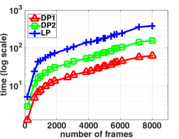
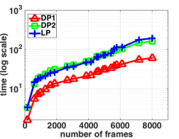
We conduct cross-validation experiments on the training set for MOT and KITTI benchmarks to study the effect of quadratic terms, loss function and inference algorithm. The results are summarized in Table 1 and 2. As shown in right side of Table 1, our novel loss function is superior to traditional Hamming loss in terms of maximizing MOTA. The 1-pass DP proposed in section 4 achieves up to 10x speedup with negligible loss in most metrics; 2-pass DP performs better than 1-pass DP in most metrics, while still being up to 3x faster than LP inference (Figure 6) on long video sequence with dense objects.

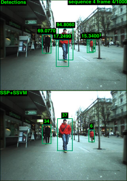
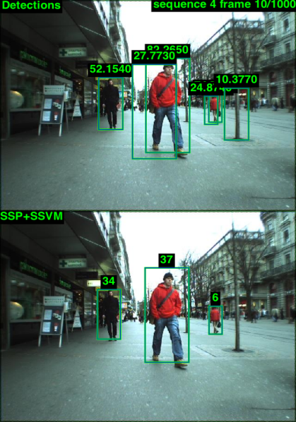
We found SSP (min-cost flow without quadratic terms) achieves slightly better overall accuracy on the MOT dataset. MOT only contains a single object category and includes videos from many different viewpoints (surveillance, vehicle, street level) which limits the potential benefits of simple 2D context features. However, by properly learning the detector confidence and transition smoothness in the SSP model, many false tracks can be pruned even without contextual knowledge.

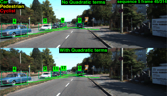
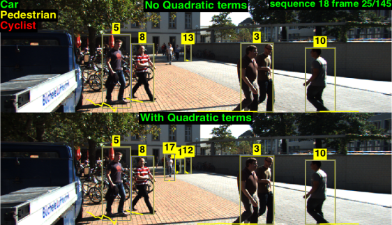
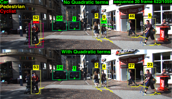
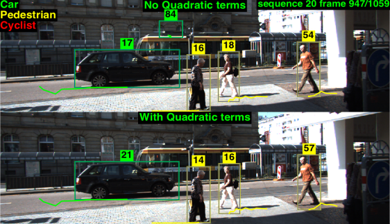
For traditional multi-category detector such as DPM, quadratic interactions were very helpful to improve the tracking performance on KITTI; this is most evident for tracking cyclist, as shown in Table 2, where LP, DP1 and DP2 all achieve considerable improvement over the baseline linear objective.

However, when we switch to the much more accurate regionlet detector on KITTI, LP inference achieves only slightly better results than SSP on car and pedestrian, while losing to SSP on cyclist category. This is very similar to the result on MOT dataset, where the LP and SSP models achieve almost equivalent results. We attribute this to the increasingly accurate regionlet detector squeezing out any relative gains to be had from our simple quadratic interactions. Interestingly, the gap between LP and the 1-pass DP approximation is also larger. Since the regionlet detector can often find objects with extreme occlusion and truncation, the tracking graph can become quite complicated and using one-shot greedy decisions for tracks can lead to inferior tracking result. Two-pass DP, with its ability to “fix” potential errors from previously found tracks, outperforms 1-pass DP by a noticeable margin in this scenario.

7.5 Integrality Gap for Greedy Dynamic Programming

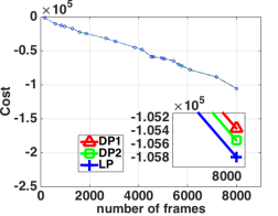
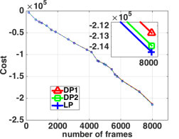
We compare the accumulated cost from DP1, DP2, LP and the relaxed optimum on 21 training sequences of KITTI dataset. The visual comparison, as well as the exact numbers are reported in Fig 6. We note that the LP method often produces integral results even before rounding. This may be in part because the the structured SVM will tend penalize fractional solution resulting in learned model parameters that favors integral results. On the other hand, DP1 and DP2 which are greedy algorithms, do not benefit from this specific property of structured SVM but they still manage to find good approximation within 1% of the relaxed optimum.

We note that there are two ways in which the “greedy” dynamic programming can be suboptimal. First, without quadratic interactions, the dynamic programming approach only approximately optimizes the min-cost flow objective. This optimality gap only appears when tracks that would have been found correctly by SSP cross in the video sequence. When there are no crossings, 1-pass greedy DP will find globally optimal solution, and in most real-world tracking scenarios, 2-pass greedy DP is sufficient to fix most of the “errors” 1-pass DP could have made.

Second, for models with quadratic interactions, the greedy DP approach may instance a single track when it might have been better (lower cost) to instance a pair of tracks which have negative or zero interactions with each other while each having strong positive interactions with the greedily instanced track (remember we are minimizing the objective). Greedy selection algorithms have some optimality guarantees in the case of submodular set functions (i.e.strictly positive pairwise interactions for the minimization problem). However, the theoretical bounds are quite loose. Empirically, we observe that the integrality gap between the LP relaxation and integral solutions produced by greedy DP are often within 1% of the relaxed optimum, as shown in Fig 6.

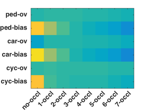
(a) inter-frame weights	(b) intra-frame weights

Figure 5: Visualization of the weight vector learned on KITTI dataset for the DPM detector. Yellow has small cost, blue has large cost. (a) shows transition weights for different length of frame jumps. (b) shows learned pairwise contextual weights between objects. The model encourages intra-class co-occurrence when objects are close but penalizes overlap and objects on top of others. Note the strong negative interaction learned between cyclist and pedestrian (two classes which are easily confused by their respective detectors.). Figure is best viewed in color.

(a) KITTI-DPM Speed	(b) KITTI-Regionlet Speed
(c) KITTI-DPM Cost	(d) KITTI-Regionlet Cost

DPM detections
Method	Time(seconds)	Time(FPS)	Cost
DP1	62.5	128.1	-105356.636294
DP2	157.4	50.9	-105535.299785
LP	384.9	20.8	-105788.159640
Relax	NA	NA	-105788.871516
Regionlet detections
Method	Time(seconds)	Time(FPS)	Cost
DP1	60.7	131.9	-212669.923615
DP2	162.4	49.3	-213873.592597
LP	192.7	41.6	-214483.825168
Relax	NA	NA	-214484.227818
(e) Detailed running time and cost

Figure 6: Speed and quality comparison of proposed DP and traditional LP approximation over 21 sequences of KITTI training set. (a) and (b) are running time comparisons. Both DP1 and DP2 run much faster than LP inference, with DP1 being up to 10x faster on specific videos. (c) and (d) are cost comparisons. Notice that DP2 always finds lower total cost than DP1, which often results in better tracking performance (see Section 7.4 for details). Figures are best viewed in color. Running times are averaged over three separate runs of each instance.

Figure 7: Additional Qualitative Results on KITTI DPM detection set. With help of intra-class quadratic interactions, the tracker is able to instantiate more correct trajectories.

Figure 8: Additional Qualitative Results on KITTI DPM detection set. The linear cost tracking model has wrongly labeled “a person pushing a cart” as “cyclist” (top-left), while our quadratic model is able to suppress cyclist trajectory with a high penalty between co-occurrence of pedestrian and cyclist (bottom-left). The quadratic interaction is also helpful in that it could help to suppress spatially infeasible co-occurrence from imperfect detectors, such as a car appearing on the back of a pedestrian (left), or a car “flying” above a pedestrian (right).

Figure 9: By learning a proper parameter set, even a network-flow model without pairwise potentials can prune away many false tracks by reasoning about detection confidence and transition smoothness.

7.6 Running Time

We show running time comparison among DP1, DP2 and LP on KITTI training set in Figure 6. For LP we only count the time spent inside MOSEK library for relaxed inference, Frank-Wolfe rounding, plus the time for backtracking final tracks. For DP1 and DP2 we count the entire period spent inside our MATLAB function. On the DPM detection set, both DP1 and DP2 run much faster than LP, with DP1 being up to 10x faster and DP2 up to 3x faster. On regionlet detection set, the gap between DP2 and LP becomes smaller, this is most likely due to the fact that regionlet detection set has fewer candidate detections per sequence than DPM set, and the overhead of MATLAB implementation comes to dominate. In fact, for sequence 17 and sequence 20, on which both DP2 and LP take more than 10 seconds to finish using regionlet detections, DP2 runs 2x and 1.5x faster than LP, respectively.

We note that our current implementation is not heavily optimized. For example, the dynamic programming step in our DP2 implementation only takes up to 50% of the total running time while contextual updates take up the remainder. This suggests there is plenty of room to further accelerate and optimize the DP algorithms.

8 Conclusion and Future Work

We have described algorithms for multi-target track association with quadratic interactions that are a natural extension of previously published approaches (Zhang et al (2008); Pirsiavash et al (2011)). Surprisingly, the resulting system is able to outperform many far more complex state-of-the-art methods on both MOT and KITTI benchmarks. In contrast, simple application of the DP-based tracker described by Pirsiavash et al (2011) does quite poorly on these datasets (e.g., MOTA=14.9 on the MOT benchmark). We attribute the performance boost to our learning framework which produces much better parameters than those estimated by hand-tuning or piece-wise model training.

A basic assumption of the network-flow models is that the entire video is available. However it can become online by simply solving a new network-flow problem every time we get a new frame; this might sound expensive at first, but remember that we can use the caching strategy described in Section 4.2.4 to save the effort of computing the first pass of dynamic programming, which is often the most time-consuming one. Lenz et al (2015) describes an online successive-shortest-path algorithm with fixed size of memory, in which they fix the solution for nodes beyond a certain number of frames. Obviously, our DP algorithms can do the same to achieve online inference with bounded memory.

We stress that the ideas described here is also complimentary to other existing methods. While we did not see significant benefits to adding simple appearance-based affinity features (e.g., RGB histogram or HOG) to our model, many state-of-the-art systems perform hierarchical or streaming data association which involves collecting examples from extended period of trajectory to train target specific appearance models in an online fashion. Such improved appearance models can be adapted to our framework, providing a way to explore more complicated affinity features while estimating hyper-parameters automatically from data. One could also introduce richer, trajectory level contextual features under such a hierarchical learning framework.

References

- Ahuja et al (1993) Ahuja RK, Magnanti TL, Orlin JB (1993) Network Flows: Theory, Algorithms, and Applications. Prentice-Hall, Inc., Upper Saddle River, NJ, USA
- Bae and Yoon (2014) Bae SH, Yoon KJ (2014) Robust online multi-object tracking based on tracklet confidence and online discriminative appearance learning. In: Proc. of CVPR
- Bernardin and Stiefelhagen (2008) Bernardin K, Stiefelhagen R (2008) Evaluating multiple object tracking performance: The clear mot metrics. Journal on Image Video Processing DOI 10.1155/2008/246309
- Brau et al (2013) Brau E, Guan J, Simek K, Del Pero L, Reimer Dawson C, Barnard K (2013) Bayesian 3d tracking from monocular video. In: Proc. of ICCV
- Brendel et al (2011) Brendel W, Amer M, Todorovic S (2011) Multiobject tracking as maximum weight independent set. In: Proc. of CVPR
- Butt and Collins (2013) Butt AA, Collins RT (2013) Multi-target tracking by lagrangian relaxation to min-cost network flow. In: Proc. of CVPR
- Chari et al (2015) Chari V, Lacoste-Julien S, Laptev I, Sivic J (2015) On pairwise costs for network flow multi-object tracking. In: Proc. of CVPR
- Choi (2015) Choi W (2015) Near-online multi-target tracking with aggregated local flow descriptor. In: Proc. of ICCV
- Choi and Savarese (2012) Choi W, Savarese S (2012) A unified framework for multi-target tracking and collective activity recognition. In: Proc. of ECCV
- Dehghan et al (2015) Dehghan A, Tian Y, Torr PH, Shah M (2015) Target identity-aware network flow for online multiple target tracking. In: Proc. of CVPR
- Desai et al (2009) Desai C, Ramanan D, Fowlkes C (2009) Discriminative models for multi-class object layout. In: Proc. of ICCV
- Dollár et al (2014) Dollár P, Appel R, Belongie S, Perona P (2014) Fast feature pyramids for object detection. IEEE Transactions on Pattern Analysis and Machine Intelligence 36(8):1532–1545
- Felzenszwalb et al (2010) Felzenszwalb PF, Girshick RB, McAllester D, Ramanan D (2010) Object detection with discriminatively trained part based models. IEEE Transactions on Pattern Analysis and Machine Intelligence 32(9):1627 – 1645
- Finley and Joachims (2008) Finley T, Joachims T (2008) Training structural SVMs when exact inference is intractable. In: Proc. of ICML
- Geiger et al (2012) Geiger A, Lenz P, Urtasun R (2012) Are we ready for autonomous driving? the kitti vision benchmark suite. In: Proc. of CVPR
- Geiger et al (2013) Geiger A, Lenz P, Stiller C, Urtasun R (2013) Vision meets robotics: The kitti dataset. International Journal of Robotics Research 32(11):1231–1237
- Geiger et al (2014) Geiger A, Lauer M, Wojek C, Stiller C, Urtasun R (2014) 3d traffic scene understanding from movable platforms. IEEE Transactions on Pattern Analysis and Machine Intelligence 36(5):1012 – 1025
- Joachims et al (2009) Joachims T, Finley T, Yu CN (2009) Cutting-plane training of structural svms. Machine Learning 77(1):27–59
- Joulin et al (2014) Joulin A, Tang K, Fei-Fei L (2014) Efficient image and video co-localization with frank-wolfe algorithm. In: Proc. of ECCV
- Kim et al (2015) Kim C, Li F, Ciptadi A, Rehg JM (2015) Multiple hypothesis tracking revisited. In: Proc. of ICCV
- Kim et al (2013) Kim S, Kwak S, Feyereisl J, Han B (2013) Online multi-target tracking by large margin structured learning. In: Proc. of ACCV
- Lacoste-Julien et al (2006) Lacoste-Julien S, Taskar B, Klein D, Jordan MI (2006) Word alignment via quadratic assignment. In: Proc. of HLT-NAACL
- Leal-Taixé et al (2014) Leal-Taixé L, Fenzi M, Kuznetsova A, Rosenhahn B, Savarese S (2014) Learning an image-based motion context for multiple people tracking. In: Proc. of CVPR
- Leal-Taixé et al (2015) Leal-Taixé L, Milan A, Reid I, Roth S, Schindler K (2015) MOTChallenge 2015: Towards a benchmark for multi-target tracking. arXiv:150401942 [cs]
- Lenz et al (2015) Lenz P, Geiger A, Urtasun R (2015) Followme: Efficient online min-cost flow tracking with bounded memory and computation. In: Proc. of ICCV
- Li et al (2009) Li Y, Huang C, Nevatia R (2009) Learning to associate: Hybridboosted multi-target tracker for crowded scene. In: Proc. of CVPR
- Liu (2009) Liu C (2009) Beyond pixels: Exploring new representations and applications for motion analysis. PhD thesis, Massachusetts Institute of Technology
- Lou and Hamprecht (2011) Lou X, Hamprecht FA (2011) Structured learning for cell tracking. In: Proc. of NIPS
- Milan et al (2012) Milan A, Schindler K, Roth S (2012) Discrete-continuous optimization for multi-target tracking. In: Proc. of CVPR
- Milan et al (2013) Milan A, Schindler K, Roth S (2013) Detection- and trajectory-level exclusion in multiple object tracking. In: Proc. of CVPR
- Milan et al (2014) Milan A, Roth S, Schindler K (2014) Continuous energy minimization for multitarget tracking. IEEE Transactions on Pattern Analysis and Machine Intelligence 36(1):58–72
- Milan et al (2015) Milan A, Leal-Taixé L, Schindler K, Reid I (2015) Joint tracking and segmentation of multiple targets. In: Proc. of CVPR
- Milan et al (2016) Milan A, Schindler K, Roth S (2016) Multi-target tracking by discrete-continuous energy minimization. IEEE Transactions on Pattern Analysis and Machine Intelligence 38(10):2054 – 2068
- Pirsiavash et al (2011) Pirsiavash H, Ramanan D, Fowlkes CC (2011) Globally-optimal greedy algorithms for tracking a variable number of objects. In: Proc. of CVPR
- Segal and Reid (2013) Segal AV, Reid I (2013) Latent data association: Bayesian model selection for multi-target tracking. In: Proc. of ICCV
- Solera et al (2015) Solera F, Calderara S, Cucchiara R (2015) Learning to divide and conquer for online multi-target tracking. In: Proc. of ICCV
- Szummer et al (2008) Szummer M, Kohli P, Hoiem D (2008) Learning crfs using graph cuts. In: ECCV
- Tang et al (2013) Tang S, Andriluka M, Milan A, Schindler K, Roth S, Schiele B (2013) Learning people detectors for tracking in crowded scenes. In: Proc. of ICCV
- Tang et al (2015) Tang S, Andres B, Andriluka M, Schiele B (2015) Subgraph decomposition for multi-target tracking. In: Proc. of CVPR
- Taskar et al (2003) Taskar B, Guestrin C, Koller D (2003) Max-margin markov networks. In: Proc. of NIPS
- Wang et al (2014) Wang B, Wang G, Luk Chan K, Wang L (2014) Tracklet association with online target-specific metric learning. In: Proc. of CVPR
- Wang and Fowlkes (2015) Wang S, Fowlkes CC (2015) Learning optimal parameters for multi-target tracking. In: Proc. of BMVC
- Wang et al (2013) Wang X, Yang M, Zhu S, Lin Y (2013) Regionlets for generic object detection. In: Proc. of ICCV
- Wu et al (2012) Wu Z, Thangali A, Sclaroff S, , Betke M (2012) Coupling detection and data association for multiple object tracking. In: Proc. of CVPR
- Xiang et al (2015) Xiang Y, Alahi A, Savarese S (2015) Learning to track: Online multi-object tracking by decision making. In: Proc. of ICCV
- Yang and Nevatia (2012) Yang B, Nevatia R (2012) An online learned crf model for multi-target tracking. In: Proc. of CVPR
- Yoon et al (2015) Yoon JH, Yang M, Lim J, Yoon K (2015) Bayesian multi-object tracking using motion context from multiple objects. In: Proc. of WACV
- Zaied and Shawky (2014) Zaied ANH, Shawky LAE (2014) A survey of quadratic assignment problems. International Journal of Computer Applications 101(6):28–36
- Zhang et al (2008) Zhang L, Li Y, Nevatia R (2008) Global data association for multi-object tracking using network flows. In: Proc. of CVPR