Theoretical description of mixed-field orientation of asymmetric top molecules: a time-dependent study

Abstract

We present a theoretical study of the mixed-field-orientation of asymmetric top molecules in tilted static electric field and non-resonant linearly polarized laser pulse by solving the time-dependent Schrödinger equation. Within this framework, we compute the mixed-field orientation of a state selected molecular beam of benzonitrile (C₇H₅N) and compare with the experimental observations Hansen et al. (2011), and with our previous time-independent descriptions Omiste et al. (2011a). For an excited rotational state, we investigate the field-dressed dynamics for several field configurations as those used in the mixed-field experiments. The non-adiabatic phenomena and their consequences on the rotational dynamics are analyzed in detail.

I Introduction

During the last years, experimental efforts have been undertaken to develop and improve experimental techniques to enhance the orientation of polar molecules Holmegaard et al. (2009); Nevo et al. (2009); Frumker et al. (2012); Trippel et al. (2013); Mun et al. (2014); Kraus et al. (2014). When a molecule is oriented the molecular fixed axes are confined along the laboratory fixed axes and its permanent dipole moment possesses a well defined direction. The experimental efforts are motivated by the broad range of promising perspectives and possible applications of oriented molecules, such as high-order harmonic generation Peng et al. (2013); Zhang et al. (2015); Li et al. (2016), chemical reaction dynamics Loesch and Möller (1992); Rakitzis et al. (2004); Ospelkaus et al. (2010); Quéméner and Bohn (2010), ultracold molecule-molecule collision dynamics Loesch and Remscheid (1990); Ni et al. (2010); Henson et al. (2012); Vogels et al. (2015), and diffractive imaging of polyatomic molecules Yamazaki et al. (2015); Kierspel et al. (2015).

The theoretical prediction to strongly orient molecules by coupling the quasidegenerate levels of a non-resonant-laser generated pendular state Friedrich and Herschbach (1999a, b), quickly became a promising experimental technique Baumfalk et al. (2001); Sakai et al. (2003); Tanji et al. (2005). However, only using state-selected ensembles of linear and asymmetric top molecules unprecedented degrees of orientation could be reached Holmegaard et al. (2009); Filsinger et al. (2009); Nevo et al. (2009); Ghafur et al. (2009). These experimental efforts have been accompanied of theoretical studies to provide a better physical insight into the field-dressed dynamics. For a state-selected beam of asymmetric top molecules, the first analysis showed that the experimental mixed-field orientation could not be reproduced in an adiabatic description Omiste et al. (2011a). Based on the lack of azimuthal symmetry due to the weak static electric field, a diabatic model was proposed to classify the avoided crossing as diabatic and adiabatic depending on the field-free magnetic quantum numbers of the involved states Omiste et al. (2011a). An explicit time-dependent analysis of the mixed-field-orientation experiments of OCS concluded that this process is, in general, non-adiabatic and requires a time-dependent quantum-mechanical description Nielsen et al. (2012). The lack of adiabaticity is due to the formation of the quasidegenate pendular doublets as the laser intensity is increased, the resulting narrow avoided crossings, and the corresponding couplings between the states in a $|J,M\rangle$ manifold for tilted fields Nielsen et al. (2012); Omiste and González-Férez (2012). These non-adiabatic phenomena provoke a transfer of population between energetically neighboring adiabatic pendular states, which might significantly reduce the degree of orientation Nielsen et al. (2012); Omiste and González-Férez (2012), this effect can be mitigated using stronger dc electric fields Kienitz et al. . This population transfer between the oriented and anti-oriented states forming a pendular doublet could be efficiently controlled to achieve a strong field-free orientation during the post-pulse dynamics Trippel et al. (2015).

For an asymmetric top molecule, we had performed a first time-dependent study on parallel fields showing the complexity of the field-dressed dynamics Omiste and González-Férez (2013). Here, we extend this work and analyze the rotational dynamics of benzonitrile (BN) in tilted-field configurations similar to those used in current mixed-field experiments. Within this time-dependent framework, we revisit the experiment on mixed-field orientation of a state-selected molecular beam of benzonitrile Hansen et al. (2011); Holmegaard et al. (2010), extending upon our earlier theoretical description Omiste et al. (2011a). The sources of discrepancies between the experimental results and the time-dependent description are analyzed. For a prototypical excited rotational state, we explore the field-dressed rotational dynamics and investigate the complicated non-adiabatic phenomena, showing that it is experimentally more challenging to reach the adiabatic limit.

The paper is organized as follows: In Sec. II we present the Hamiltonian of a polar asymmetric top molecule in tilted electric and non-resonant laser fields, and the numerical method used to solve the time-independent Schrödinger equation. The time-dependent description of the mixed-field orientation experiment of a benzonitrile molecular beam is presented in Sec. III, where we also provide a comparison with our previous time-independent analysis. Section IV is devoted to investigate the mixed-field dynamics of an excited rotational state, and we explore the sources of non-adiabatic effects in Sec. V. The conclusions are given in Sec. VI.

II The Hamiltonian of an asymmetric top molecule in tilted fields

We consider a polar asymmetric top molecule in combined electric and non-resonant laser fields. Our study is restricted to asymmetric top molecules that can be described within the rigid rotor approximation, and that have the polarizability tensor diagonal in the principal axes of inertia frame and the permanent electric dipole moment $\mathbf{\mu}$ parallel to the $z$-axis of this molecule fixed frame (MFF) $(x,y,z)$. The MFF $z$-axis is taken along the molecular axis with the smallest moment of inertia. The non-resonant laser field is linearly polarized along the $Z$-axis of the laboratory fixed frame (LFF) $(X,Y,Z)$ and the electric field is tilted by an angle $\beta$ with respect to the LFF $Z$-axis and contained in the $XZ$-plane. The rotational dynamics of the molecule is described using the Euler angles $(\theta,\phi,\chi)$ that relate the LFF and MFF Zare (1988). In the framework of the rigid rotor approximation, the Hamiltonian reads as

$$H(t)=H_{R}+H_{s}(t)+H_{L}(t),$$ ((1))

where $H_{R}$ is the field-free rotational Hamiltonian

$$H_{R}=B_{x}{J}_{x}^{2}+B_{y}{J}_{y}^{2}+B_{z}{J}_{z}^{2}$$ ((2))

with ${J}_{k}$ being the projection of the total angular momentum operator $\mathbf{J}$ along the MFF $k$-axis with $k=x,y$, and $z$, and $B_{k}$ the rotational constant along the MFF $k$-axis. For BN, the rotational constants are $B_{x}=1214$ MHz, $B_{y}=1547$ MHz and $B_{z}=5655$ MH Wohlfart et al. (2007).

The electric field $\mathbf{\text{E}}_{s}(t)$ interacts with the electric dipole moment $\mathbf{\mu}$ of the molecule as

$$H_{s}(t)=-\mu\text{E}_{s}(t)\cos\theta_{s},$$ ((3))

where $\theta_{s}$ is the angle between the electric field and the MFF $z$-axis, $\cos\theta_{s}=\cos\theta\cos\beta+\sin\beta\sin\theta\cos\phi$. For BN, the permanent electric dipole moment is $\mu=4.515$ D Wohlfart et al. (2007). $\text{E}_{s}(t)$ initially depends linearly on time, and once the maximum strength $\text{E}_{s}$ is reached, it is kept constant. The turning on speed ensures that the process is adiabatic, and we have neglected the coupling of this field with the molecular polarizability or higher order terms.

For a non-resonant linearly polarized laser field, the interaction reads Seideman and Hamilton (2006); Omiste et al. (2011b)

$$H_{L}(t)=-\cfrac{\textup{I}(t)}{2\epsilon_{0}c}\left(\alpha^{zx}\cos^{2}\theta+\alpha^{yx}\sin^{2}\theta\sin^{2}\chi\right),$$ ((4))

where $\alpha^{km}=\alpha_{kk}-\alpha_{mm}$ are the polarizability anisotropies, and $\alpha_{kk}$ the polarizability along the molecular $k$-axis $k,m=x,y$ and $z$. For BN, the polarizabilities are $\alpha_{xx}=7.49$ Å³, $\alpha_{yy}=13.01$ Å³ and $\alpha_{zz}=18.64$ Å³ Wohlfart et al. (2007). $\epsilon_{0}$ is the dielectric constant and $c$ the speed of light. In this work, we consider Gaussian pulses with intensity $\textup{I}(t)=\textup{I}_{0}\exp\left(-\cfrac{4\ln 2t^{2}}{\tau^{2}}\right)$, $\textup{I}_{0}$ is the peak intensity and $\tau$ is the full width half maximum (FWHM).

For tilted fields with $\beta\neq 0^{\circ},\,90^{\circ},\,180^{\circ}$, the symmetries of the rigid rotor Hamiltonian ((1)) are the identity, $E$, the two fold rotation around the MFF $z$-axis, $C_{z}^{2}$, and the reflections $\sigma_{XZ}$ on the plane spanned by the two fields, i. e., the $XZ$-plane. These symmetries imply the conservation of the parity of the projection of $\mathbf{J}$ on the MFF $z$-axis, i. e., the parity of $K$, and the parity under the reflections on the LFF $XZ$-plane $\sigma_{XZ}$. Consequently, the eigenstates can be classified in four different irreducible representations Omiste et al. (2011b), whose basis elements are presented in Table 1 in terms of the field-free symmetric top eigenstates $|JKM\rangle$ Omiste et al. (2011b).

Parity			Functions
$C_{z}^{2}$	$\sigma_{XZ}$	$K$
$e$	$e$	$e$, $K,M=0$	$\left|J00\right\rangle$
$e$	$e$	$e$	$\frac{1}{\sqrt{2}}\left(|JKM\rangle+(-1)^{K+M}|J-K-M\rangle\right)$
$e$	$o$	$e$	$\frac{1}{\sqrt{2}}\left(|JKM\rangle+(-1)^{K+M+1}|J-K-M\rangle\right)$
$o$	$e$	$o$	$\frac{1}{\sqrt{2}}\left(|JKM\rangle+(-1)^{K+M}|J-K-M\rangle\right)$
$o$	$o$	$o$	$\frac{1}{\sqrt{2}}\left(|JKM\rangle+(-1)^{K+M+1}|J-K-M\rangle\right)$

Table 1: For tilted fields with $\beta\neq 90^{\circ}$, functions used in the basis set expansion of the time-dependent wave function.

The time-dependent Schrödinger equation associated with the Hamiltonian (1) is solved combining the short iterative Lanczos method Beck et al. (2000) for the time variable and a basis set expansion in the field-free top eigenstates written in terms of the Wang states, $\left|JKM\right\rangle$, for the angular coordinates. For each irreducible representation, the symmetric top wave functions forming the basis are properly symmetrized as indicated in Table 1 Omiste et al. (2011b). The time-dependent wave function is labeled using the adiabatic following and the field-free notation $\left|J_{K_{a},K_{c}}M\right>_{\text{t}}$ where $K_{a}$ and $K_{c}$ are the values of $K$ for the limiting prolate and oblate symmetric top rotor, respectively King et al. (1943).

To analyze the rotational dynamics, the time-dependent wave function is projected on the adiabatic pendular states at time $t$

$$\left|J_{K_{a},K_{c}}M\right>_{\text{t}}=\sum C_{\left|{\cal J}_{{\cal K}_{a},{\cal K}_{c}}\cal{M}\right>}(t)\left|{\cal J}_{{\cal K}_{a},{\cal K}_{c}}\cal{M}\right>_{\text{p}}$$ ((5))

with $C_{\left|{\cal J}_{{\cal K}_{a},{\cal K}_{c}}\cal{M}\right>}(t)={}_{\textup{p}}\left<\right.{\cal J}_{{\cal K}_{a}{\cal K}_{c}}{\cal{M}}\left|J_{K_{a},K_{c}}M\right>_{\text{t}}$ and the wave function of the adiabatic pendular state of the instantaneous Hamiltonian ((1)) $\left|{\cal J}_{{\cal K}_{a},{\cal K}_{c}}\cal{M}\right>_{\text{p}}$ that connects adiabatically to the field-free state $\left|{\cal J}_{{\cal K}_{a},{\cal K}_{c}}\cal{M}\right>$. The sum in Eq. (5) runs over all pendular states within the same irreducible representation.

The rotational dynamics can be characterized by the adiabaticity ratio or parameter Ballentine (1998)

$$\eta=\cfrac{\hbar\left|\tensor{[}_{\textup{p}}]{\left\langle k\left|\cfrac{\partial H_{\textup{L}}(t)}{\partial t}\right|m\right\rangle}{{}_{\textup{p}}}\right|}{\left|E_{m}-E_{k}\right|^{2}}$$ ((6))

where $\left|k\right\rangle_{\text{p}}$ and $\left|m\right\rangle_{\text{p}}$ are the eigenfunctions of the adiabatic pendular eigenstates of Hamiltonian (1) at time $t$ and $E_{k}$ and $E_{m}$ are the eigenenergies. The rotational dynamics can be considered as adiabatic at a certain time if $\eta\ll 1$ Ballentine (1998).

II.1 Experimental measures

In mixed-field orientation experiments, the degree of orientation can be measured by a multiple-ionization and a subsequent Coulomb explosion of the molecule, and the velocity mapping of the ionic fragments onto a 2D screen perpendicular to the dc field of the velocity mapping electrodes. The molecular orientation is reflected in the 2D-images, which show an up/down asymmetry measured by the ratio $\text{N}_{\text{up}}/\text{N}_{\text{tot}}$, where $\text{N}_{\text{tot}}$ and $\text{N}_{\text{up}}$ stand for the amount of ions collected on the full screen and on its upper part, respectively, Holmegaard et al. (2009); Filsinger et al. (2009); Nevo et al. (2009). Theoretically, the recorded image corresponds to the 2D projection of the 3D probability density on the screen perpendicular to the electric field Omiste et al. (2011a); Nielsen et al. (2012). The theoretical orientation ratio $\text{N}_{\text{up}}/\text{N}_{\text{tot}}$ reads

$$\text{N}_{\text{up}}/\text{N}_{\text{tot}}=\cfrac{\int_{0}^{\infty}\int_{-\infty}^{\infty}\rho(y_{s},z_{s})dy_{s}dz_{s}}{\int_{-\infty}^{\infty}\int_{-\infty}^{\infty}\rho(y_{s},z_{s})dy_{s}dz_{s}}.$$ ((7))

where $\rho(y_{s},z_{s})$ is the 2D probability density, $y_{s}$ and $z_{s}$ are the horizontal and vertical screen coordinates, respectively. Here, we derive this 2D probability density including the selectivity factor of a circularly polarized probe laser and the experimental velocity distribution of the ionic fragments under the recoil approximation Omiste et al. (2011a). Note that for non-oriented states, $\left\langle\cos\theta\right\rangle=0$ and $\text{N}_{\text{up}}/\text{N}_{\text{tot}}=0.5$, whereas $\text{N}_{\text{up}}/\text{N}_{\text{tot}}>0.5$ and $\text{N}_{\text{up}}/\text{N}_{\text{tot}}<0.5$ for oriented and antioriented states, respectively.

III Mixed-field orientation for experimental conditions

In this section we present a theoretical time-dependent description of the mixed-field orientation corresponding to previous mixed-field-orientation experiments of benzonitrile Filsinger et al. (2009), and a comparison with our previous time-independent analysis Omiste et al. (2011a). State-selected benzonitrile molecules in a molecular beam were oriented using the weak dc electric field from the velocity-map-imaging spectrometer and a non-resonant laser pulse Filsinger et al. (2009). For a $10$ ns laser pulse with peak intensity $\textup{I}_{0}=$7\text{\times}{10}^{11}\text{\,}\mathrm{W}\text{/}{\mathrm{cm}}^{2}$$ and a weak dc field, $\text{E}_{s}=$286\text{\,}\mathrm{V}\text{/}\mathrm{cm}$$, tilted with respect to each other an angle $\beta=135^{\circ}$, the experimentally measured degree of orientation was $\text{N}_{\text{up}}/\text{N}_{\text{tot}}=0.71$ Hansen et al. (2011). For this field configuration, we perform a theoretical study including $54$ rotational states of the state-selected molecular beam of this experiment, i. e., accounting for $92.5\%$ of the total population in the beam Hansen et al. (2011).

The adiabatic approximation, which assumes that the field-dressed instantaneous eigenstate is a solution of the time-dependent Hamiltonian, would give rise to a very weakly oriented ensemble with $\text{N}_{\text{up}}/\text{N}_{\text{tot}}=0.55$ Omiste et al. (2011a). This result is in contradiction with the experimental observation and indicates that the mixed-field orientation is, in general, a non adiabatic process Omiste et al. (2011a). The weak electric field is responsible for breaking the azimuthal symmetry, and for coupling states with different field-free magnetic quantum numbers. Based on this fact, we had proposed a diabatic model Omiste et al. (2011a), which improves the adiabatic description by classifying the avoided crossings: as $\textup{I}(t)$ increases, they are crossed diabatically (adiabatically) if the involved states have different (same) field-free expectation value $\left\langle M^{2}\right\rangle$. The diabatic model is equivalent to an adiabatic description of a parallel field configuration including only the dc electric field component parallel to the alignment laser field $\text{E}_{s}\cos\beta$, and neglecting the perpendicular component. Within this diabatic model, the orientation ratio of the state-selected molecular beam is $\text{N}_{\text{up}}/\text{N}_{\text{tot}}=0.624$, which is larger than for the pure adiabatic description, but still smaller than the experimental measurement.

To check the validity of the diabatic model, we have solved the time-dependent Schrödinger equation considering a dc field parallel to the LFF $Z$-axis with strength $\text{E}_{s}\cos\beta$. Hence, the field-dressed rotational dynamics takes into account the non-adiabatic couplings between states with the same magnetic quantum number and the pendular doublets formation Omiste and González-Férez (2013). In this description, we obtain a smaller orientation ratio $\text{N}_{\text{up}}/\text{N}_{\text{tot}}=0.623$ than the experimentally measured. For a full non-adiabatic description, we have taken into account all the couplings, and, in particular, those between states with different field-free magnetic quantum numbers, which were neglected in the parallel-field time-dependent description, and solved the time-dependent Schrödinger equation associated to Hamiltonian ((1)) for each initially populated state. The obtained degree of orientation $\text{N}_{\text{up}}/\text{N}_{\text{tot}}=0.612$ is still lower than the experimental one, and even lower than the simplified models described above. The discrepancies between the time-dependent descriptions of the tilted and parallel fields configurations arise due to the couplings between the states within the $\left|J_{K_{a},K_{c}}M\right>$-manifold with $0\leq M\leq J$, i. e., degenerate states in the field-free case, which differ in the magnetic quantum number $M$, at weak laser intensities, i. e., $I\lesssim$1\text{\times}{10}^{18}\text{\,}\mathrm{W}\text{/}{\mathrm{cm}}^{2}$$, and between the states with different field-free magnetic quantum numbers at strong intensities Omiste and González-Férez (2012).

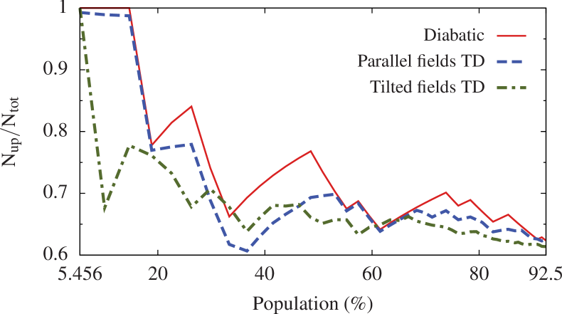
To analyze these theoretical results, we build up the molecular ensemble by successively adding states according to their populations in the experimental state-selected beam. The orientation ratio $\text{N}_{\text{up}}/\text{N}_{\text{tot}}$ is plotted in Fig. 1 versus the percentage of population included in the experimental molecular beam. For the ground state, which has the largest population, we obtain $\left\langle\cos\theta\right\rangle=0.986$ and $\text{N}_{\text{up}}/\text{N}_{\text{tot}}=0.999$, which is very close to the adiabatic result $\text{N}_{\text{up}}/\text{N}_{\text{tot}}=1$. As more states are included in the ensemble, the orientation ratio $\text{N}_{\text{up}}/\text{N}_{\text{tot}}$ decreases with a superimposed oscillatory behavior due to the orientation or antiorientation of the additionally included states. The discrepancies between these results illustrate the importance of performing a full time-dependent description of the mixed field orientation process.

Figure 1: The theoretical orientation ratio $\text{N}_{\text{up}}/\text{N}_{\text{tot}}$ as a function of the population of the molecular beam of benzonitrile using a probe laser circularly polarized perpendicular to the screen computed by the diabatic model (red solid line), by time-dependent (TD) description for parallel-fields (blue dashed line) and time-dependent description for tilted-fields (green dot-dashed line). The field configuration is $\textup{I}_{0}=$7\text{\times}{10}^{11}\text{\,}\mathrm{W}\text{/}{\mathrm{cm}}^{2}$$, $\text{E}_{s}=$286\text{\,}\mathrm{V}\text{/}\mathrm{cm}$$ and $\beta=135^{\circ}$.

Several reasons could explain the disagreement between the time-dependent study and the experimental result. First, we do not include the finite spatial profile of the alignment and probe lasers which implies that all the molecules in the beam do not feel the same laser intensity. Based on our previous studies Omiste et al. (2011a), we can conclude that this effect should not significantly modify the degree of orientation. Second, it has been assumed that the state selection along the dc-field deflector is an adiabatic process Holmegaard et al. (2009); Filsinger et al. (2009); Nevo et al. (2009), if this would not be the case, the rotational states before the mixed-field orientation experiment would not be pure field-free states. Third, the mixed-field dynamics is very sensitive to the field configuration, and small variations on it, e. g., on the pulse shape, could significantly affect these results. Finally, by adding the rest of states forming the experimental molecular beam, the theoretical degree of orientation will not approach to the experimental one. Assuming that the rest of the states are not oriented, or that half of them are fully oriented and the other half fully antioriented, the theoretical degree of orientation would be reduced to $0.605$, still far from the experimental value.

Figure 2: The 2D projection of the probability density of the state $\left|3_{0,3}1\right>_{\text{t}}$ at the peak intensity computed using (a) the adiabatic approximation, (b) the diabatic model, and (c) the time-dependent description for tilted fields. The field configuration is $\textup{I}_{0}=$7\text{\times}{10}^{11}\text{\,}\mathrm{W}\text{/}{\mathrm{cm}}^{2}$$, $\text{E}_{s}=$286\text{\,}\mathrm{V}\text{/}\mathrm{cm}$$ and $\beta=135^{\circ}$.

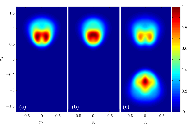
The adiabatic and diabatic approximations predict pendular states either fully oriented $\text{N}_{\text{up}}/\text{N}_{\text{tot}}\approx 1$ or antioriented $\text{N}_{\text{up}}/\text{N}_{\text{tot}}\approx 0$, whereas in a time-dependent description they are not fully oriented or fully antioriented with $0\lesssim\text{N}_{\text{up}}/\text{N}_{\text{tot}}\lesssim 1$. This is illustrated in Fig. 2 with the 2D projection of the probability density of the $\left|3_{0,3}1\right>_{\text{t}}$ state at the peak intensity. For the adiabatic and diabatic descriptions, the 2D probability density is concentrated on the upper part of the screen with $\text{N}_{\text{up}}/\text{N}_{\text{tot}}=1$. In contrast, the time-dependent description provides a weakly antioriented state with $\text{N}_{\text{up}}/\text{N}_{\text{tot}}\approx 0.44$, see Fig. 2 (c). This is due to the contributions of antioriented pendular states to the rotational dynamics: at the peak intensity the antioriented adiabatic pendular state $\left|2_{2,0}1\right>_{\text{p}}$ has the largest contribution with a weight of $41.1\%$ into the $\left|3_{0,3}1\right>_{\text{t}}$ time-dependent wave function.

IV Field-dressed dynamics of a rotational excited state

The rotational dynamics in tilted fields is more complex than in parallel fields Omiste and González-Férez (2013). We illustrate this complexity by analyzing the field-dressed dynamics of the excited state $\left|3_{0,3}1\right>$, which has been studied for parallel fields in Ref. Omiste and González-Férez (2013). For tilted fields, the adiabatic pendular state $\left|3_{0,3}1\right>_{\text{p}}$ is the ninth one of the even-even irreducible representation, and is oriented in a strong laser field combined with a weak static electric field.

Figure 3: For the $\left|3_{0,3}1\right>_{\text{t}}$ state, expectation value $\left\langle\cos\theta\right\rangle$ as a function of $\textup{I}(t)$ for laser pulses with peak intensity $\textup{I}_{0}=$7\text{\times}{10}^{11}\text{\,}\mathrm{W}\text{/}{\mathrm{cm}}^{2}$$ and temporal widths $\tau=0.5$ (red solid), $1$ (blue dashed), $5$ (orange dotted) and $10$ ns (green dot-dashed). The electric field has strength $\text{E}_{s}=$300\text{\,}\mathrm{V}\text{/}\mathrm{cm}$$, and is tilted an angle (a) $\beta=0^{\circ}$, (b) $\beta=30^{\circ}$ and (c) $\beta=60^{\circ}$.

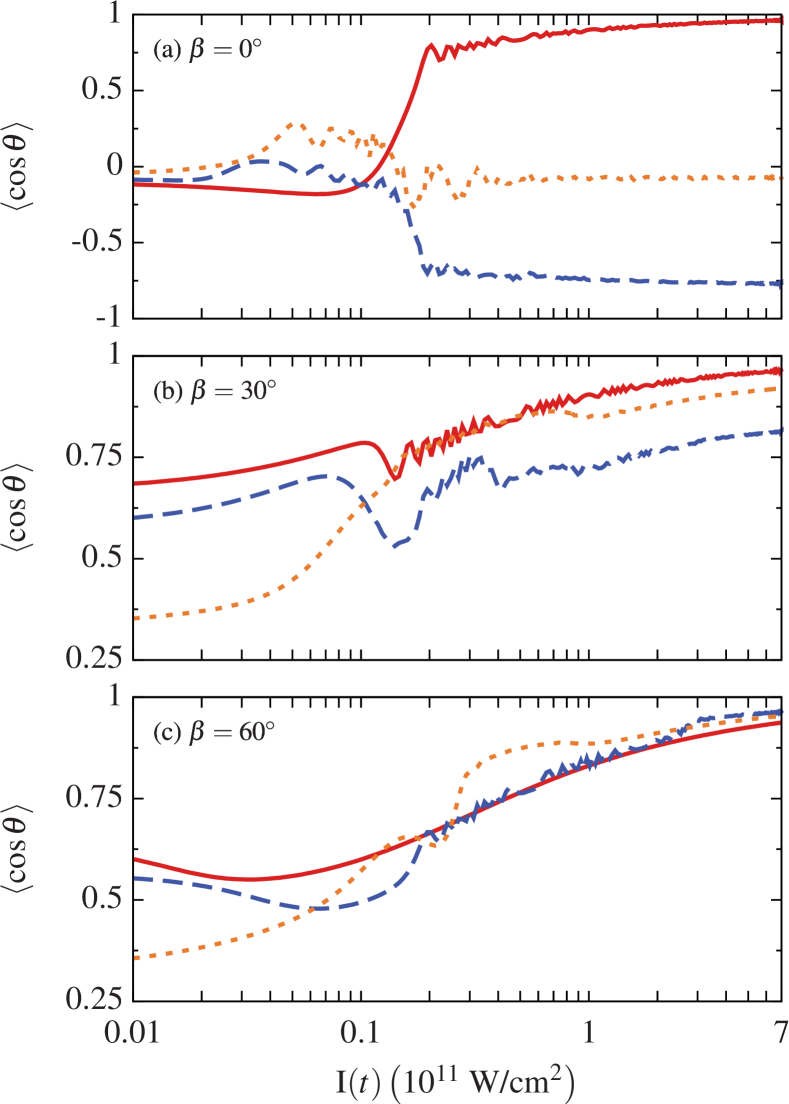
In Fig. 3 we plot the orientation $\left\langle\cos\theta\right\rangle$ of the state $\left|3_{0,3}1\right>_{\text{t}}$ as a function of the laser intensity $\textup{I}(t)$ for three different field configurations (a) $\beta=0^{\circ}$, (b) $\beta=30^{\circ}$ and (c) $\beta=60^{\circ}$, with $\text{E}_{s}=$300\text{\,}\mathrm{V}\text{/}\mathrm{cm}$$, and laser pulses with temporal widths $\tau=0.5$ ns, $1$ ns, $5$ ns and $10$ ns and peak intensity $\textup{I}_{0}=$7\text{\times}{10}^{11}\text{\,}\mathrm{W}\text{/}{\mathrm{cm}}^{2}$$. For these field configurations, the adiabatic orientation is given by $\left\langle\cos\theta\right\rangle=0.97$, and weakly affected by the inclination angle of the dc-field $\beta$.

For parallel fields, $\left|3_{0,3}1\right>_{\text{p}}$ is the third adiabatic state in the irreducible representation with $M=1$ and even parity under two-fold rotations around the MFF $z$-axis. This state is oriented in the pendular regime. As $\textup{I}(t)$ increases, the orientation shows an increasing trend with a superimposed smooth oscillatory behavior, which is due to the couplings among the adiabatic pendular states contributing to the non-adiabatic dynamics. Three adiabatic pendular states, $\left|3_{0,3}1\right>_{\text{p}}$ (oriented), $\left|2_{2,1}1\right>_{\text{p}}$ (antioriented), and $\left|2_{2,0}1\right>_{\text{p}}$ (oriented), dominantly contribute to the time-dependent wave function of $\left|3_{0,3}1\right>_{\text{t}}$. The coupling between the oriented adiabatic pendular states, i. e., $\left|3_{0,3}1\right>_{\text{p}}$ and $\left|2_{2,0}1\right>_{\text{p}}$, provokes the oscillations, because in the pendular regime their couplings with the antioriented one are close to zero, i. e., ${}_{\textup{p}}\left\langle 3_{0,3}1\left|\cos\theta\right|2_{2,2}1\right\rangle_{\textup{p}}\approx 0$ and ${}_{\textup{p}}\left\langle 2_{2,0}1\left|\cos\theta\right|2_{2,1}1\right\rangle_{\textup{p}}\approx 0$ Omiste and González-Férez (2013). The contribution of the antioriented adiabatic pendular state reduces the degree of orientation compared to the adiabatic prediction. As the temporal width of the pulse $\tau$ increases, the dynamics becomes more adiabatic and the orientation increases approaching to the adiabatic limit.

Due to the splitting of the field-free degenerate $\left|3_{0,3}M\right>$-multiplet in tilted fields, the adiabatic pendular states $\left|3_{0,3}M\right>_{\text{p}}$, with $M=0,1,2,3$, contribute to the field-dressed dynamics of $\left|3_{0,3}1\right>_{\text{t}}$ and their weights depend on the angle $\beta$ and on the dc-field strength. For $\beta=30^{\circ}$, the $\left|3_{0,3}1\right>_{\text{t}}$ wave function is antioriented, which can be rationalized in terms of the adiabatic pendular states contributing to the rotational dynamics. Once the multiplet is split, the contribution of the adiabatic pendular states $\left|3_{0,3}M\right>_{\text{p}}$ onto the $\left|3_{0,3}1\right>_{\text{t}}$ wave function is approximately the same for all the pulses. From this moment on, the way the laser is turned on plays an important role on the dynamics. We find up to $27$ adiabatic pendular states with $J\leq 4$ contributing to the dynamics of $\left|3_{0,3}1\right>_{\text{t}}$, and the antioriented adiabatic pendular state $\left|2_{2,0}1\right>_{\text{p}}$ has the largest contribution to the time-dependent wave function, larger than $67\%$ for $\tau=5$ ns and $10$ ns. By decreasing the temporal width of the pulse, more adiabatic pendular states contribute to the dynamics, and $|\left\langle\cos\theta\right\rangle|$ diminishes because the weights of oriented and antioriented adiabatic states are vey similar. In contrast, $\left|3_{0,3}1\right>_{\text{t}}$ is oriented if the dc-field is tilted an angle $\beta=60^{\circ}$. For this case, the dominant contributions to the wave function are due to the $\left|2_{2,1}2\right>_{\text{p}}$ and $\left|3_{2,1}3\right>_{\text{p}}$ oriented states for $\tau=10$ ns and $\tau=5$ ns, and to $\left|3_{2,1}3\right>_{\text{p}}$ for $\tau=1$ ns and $\tau=0.5$ ns. As $\tau$ increases, the orientation increases, but it is smaller than the adiabatic limit of the orientation $\left\langle\cos\theta\right\rangle=0.97$.

Figure 4: For the $\left|3_{0,3}1\right>_{\text{t}}$ state, expectation value $\left\langle\cos\theta\right\rangle$ as a function of $\textup{I}(t)$ for a $10$ ns laser pulse with peak intensity $\textup{I}_{0}=$7\text{\times}{10}^{11}\text{\,}\mathrm{W}\text{/}{\mathrm{cm}}^{2}$$. The electric field has strengths (a) $\text{E}_{s}=$5\text{\,}\mathrm{k\per\centi}\text{/}$$, (b) $\text{E}_{s}=$10\text{\,}\mathrm{k\per\centi}\text{/}$$, and (c) $\text{E}_{s}=$20\text{\,}\mathrm{k\per\centi}\text{/}$$, and is tilted by $\beta=0^{\circ}$ (red solid), $\beta=30^{\circ}$ (blue dashed) and $\beta=60^{\circ}$ (orange dotted).

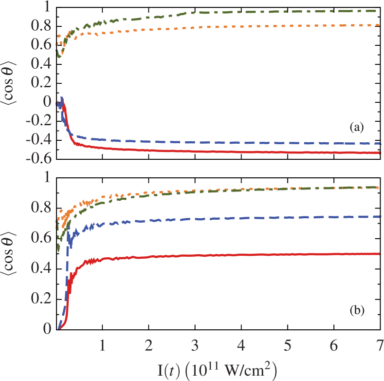
The dc-field strength determines the energy gap between the two states forming a pendular doublet in the strong laser field regime. Thus, by increasing the dc-field strength the dynamics should become more adiabatic because the population transferred between these two states as the pendular doublet is formed should be reduced. For a $10$ ns alignment pulse, we present in Fig. 4 the orientation of the $\left|3_{0,3}1\right>_{\text{t}}$ state versus the laser intensity $\textup{I}(t)$ for dc-fields strengths $\text{E}_{s}=$5\text{\,}\mathrm{k\per\centi}\text{/}$$, $\text{E}_{s}=$10\text{\,}\mathrm{k\per\centi}\text{/}$$ and $\text{E}_{s}=$20\text{\,}\mathrm{k\per\centi}\text{/}$$. Let us remark that for strong dc fields, the energy gap between two states forming the pendular doublets in a strong ac field is large and they are not quasidegenerate, and, in particular, the interaction due to the static electric field could not be treated as a perturbation to the ac-field interaction. Even for these strong electric fields, the rotational dynamics is non-adiabatic, and this state is either weakly oriented, strongly oriented or antioriented depending on the field configuration, see Fig. 4. This can be explained in terms the splitting of the $\left|3_{0,3}M\right>_{\text{p}}$ manifold and of the avoided crossings that are encountered during the time evolution of the wave packet, which, in most cases, are not crossed adiabatically Omiste and González-Férez (2013). For strong dc fields, the avoided crossings between adiabatic pendular states evolving from different multiplets become more likely. For $\text{E}_{s}=$20\text{\,}\mathrm{k\per\centi}\text{/}$$, the orientation at the peak intensity is very similar for the three tilted angles, which is due to the dominant contribution of oriented adiabatic pendular states to the rotational dynamics.

Figure 5: For the $\left|3_{0,3}1\right>_{\text{t}}$ state, expectation value $\left\langle\cos\theta\right\rangle$ as a function of $\textup{I}(t)$ for a $10$ ns laser pulse with peak intensity $\textup{I}_{0}=$7\text{\times}{10}^{11}\text{\,}\mathrm{W}\text{/}{\mathrm{cm}}^{2}$$ for (a) tilted fields with $\beta=30^{\circ}$ and for (b) parallel fields with the electric field parallel to the LFF $Z$-axis of strength $\text{E}_{s}\cos 30^{\circ}$. The electric field strengths are $\text{E}_{s}=$300\text{\,}\mathrm{V}\text{/}\mathrm{cm}$$ (red solid line), $\text{E}_{s}=$1\text{\,}\mathrm{k\per\centi}\text{/}$$ (blue dashed line), $\text{E}_{s}=$10\text{\,}\mathrm{k\per\centi}\text{/}$$ (orange dotted-line), and $\text{E}_{s}=$20\text{\,}\mathrm{k\per\centi}\text{/}$$ (green dot-dashed line)

For the $\left|3_{0,3}1\right>_{\text{t}}$ state, we compare in Fig. 5 the orientation in tilted fields with the results obtained in a parallel field configuration which includes only the $Z$-component of the electric field $\text{E}_{s}\cos\beta$. For this parallel field configuration, the state is oriented, $\left\langle\cos\theta\right\rangle$ increases as $\text{E}_{s}$ is enhanced and shows a plateau like behavior for $\textup{I}(t)\gtrsim$1\text{\times}{10}^{11}\text{\,}\mathrm{W}\text{/}{\mathrm{cm}}^{2}$$. In contrast, for tilted-fields, the $\left|3_{0,3}1\right>_{\text{t}}$ state is anti-oriented for weak dc-fields $\text{E}_{s}=$300\text{\,}\mathrm{V}\text{/}\mathrm{cm}$$ and $\text{E}_{s}=$1\text{\,}\mathrm{k\per\centi}\text{/}$$, and oriented for $\text{E}_{s}=$10\text{\,}\mathrm{k\per\centi}\text{/}$$ and $\text{E}_{s}=$20\text{\,}\mathrm{k\per\centi}\text{/}$$. The discrepancy between these results illustrates the importance of the dc-field perpendicular to the non-resonant laser. The non-adiabatic phenomena that take place for tilted fields, i. e., the splitting of the $\left|3_{0,3}M\right>_{\text{p}}$ manifold and the avoided crossing among pendular states having different field-free magnetic quantum number, strongly affect the field-dressed dynamics. For weak electric fields, the impact of these non-adiabatic effects is larger and the direction of the orientation is reversed. Whereas, for strong dc fields, they show qualitatively similar but quantitative different orientation.

V Sources of non-adiabatic effects

For tilted fields, the dynamics is characterized by the pendular doublet formation, the splitting of the degenerate $\left|J_{K_{a},K_{c}}M\right>$-multiplet at weak laser intensities, and a large amount of avoided crossings, some of them due to the tilted electric field which breaks the azimuthal symmetry. Since the formation of the pendular doublet has been discussed in detail in our work on asymmetric top molecules in parallel fields Omiste and González-Férez (2013), we focus here on exploring the other two non-adiabatic phenomena.

Let us mention that the rotational dynamics of the ground state of each irreducible representation is only affected by the pendular doublet formation, as the absolute ground state. Thus, for them, it is easy to reach the adiabatic mixed-field orientation limit Omiste and González-Férez (2013).

V.1 Coupling in the $J$-manifold

Figure 6: For the adiabatic pendular states $\left|3_{0,3}1\right>_{\text{t}}$ (black double-dot-dashed line), $\left|3_{0,3}3\right>_{\text{p}}$ (red solid line), $\left|3_{0,3}2\right>_{\text{p}}$ (blue dashed), $\left|3_{0,3}1\right>_{\text{p}}$ (orange dotted line) and $\left|3_{0,3}0\right>_{\text{p}}$ (green dot-dashed), energy and expectation value $\left\langle M^{2}\right\rangle$ for a dc field tilted $\beta=30^{\circ}$ and with strength $\text{E}_{s}=$300\text{\,}\mathrm{V}\text{/}\mathrm{cm}$$ (a) and (d), $\text{E}_{s}=$600\text{\,}\mathrm{V}\text{/}\mathrm{cm}$$ (b) and (e), and $\text{E}_{s}=$1000\text{\,}\mathrm{V}\text{/}\mathrm{cm}$$ (c) and (f). The laser pulse has $\tau=10$ ns and peak intensity $\textup{I}_{0}=$7\text{\times}{10}^{11}\text{\,}\mathrm{W}\text{/}{\mathrm{cm}}^{2}$$.

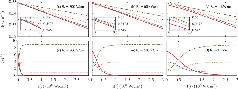
In the field-free case, the $\left|J_{K_{a},K_{c}}M\right>$ states with $0\leq M\leq J$ are degenerate due to the azimuthal symmetry. The weak electric field of the mixed-field orientation experiments breaks their $M$-degeneracy by the quadratic Stark splitting, $\Delta E\sim\text{E}_{s}^{2}$. For $\text{E}_{s}=$300\text{\,}\mathrm{V}\text{/}\mathrm{cm}$$ and $\beta=30^{\circ}$, the neighboring levels of the $\left|3_{0,3}M\right>$-manifold are separated by $1.6\times 10^{-4}$ cm^-1, $9.4\times 10^{-5}$ cm^-1 and $3.1\times 10^{-5}$ cm^-1. Due to these small energy gaps, even a weak laser field provokes strong couplings among them, which significantly affect the rotational dynamics. We consider a dc field tilted $\beta=30^{\circ}$ with strengths $\text{E}_{s}=$300\text{\,}\mathrm{V}\text{/}\mathrm{cm}$$, $600\text{\,}\mathrm{V}\text{/}\mathrm{cm}$, and $1000\text{\,}\mathrm{V}\text{/}\mathrm{cm}$. In Fig. 6 we present the energy, and expectation value $\left\langle M^{2}\right\rangle$ of the adiabatic pendular states $\left|3_{0,3}M\right>_{\text{p}}$ as the laser intensity is increased till $\textup{I}(t)=$3\text{\times}{10}^{8}\text{\,}\mathrm{W}\text{/}{\mathrm{cm}}^{2}$$. In the presence of only an electric field forming an angle $\beta$ with the LFF $Z$-axis, the projection of $\mathbf{{J}}$ along the dc-field axis is a good quantum number, but not along the LFF $Z$-axis, cf. Fig. 6 (d), (e), and (f). As the laser intensity increases, the levels suffer several avoided crossings, whose widths are larger for stronger dc-fields, see Fig. 6 (a)-(c). The effects of these avoided crossings are recognized in the time evolution of $\left\langle M^{2}\right\rangle$. After them, $\left\langle M^{2}\right\rangle$ shows a constant behavior as $\textup{I}(t)$ is increased. Indeed, when the interaction due to the laser field is dominant, the projection of $\mathbf{J}$ along the LFF $Z$-axis becomes a quasi good quantum number, as is observed in Fig. 6 (d), (e) and (f).

Figure 7: The squares of the projection of the time-dependent wave function $\left|3_{0,3}1\right>_{\text{t}}$ onto the adiabatic states of the $\left|3_{0,3}M\right>$ multiplet, i. e., $\left|3_{0,3}3\right>_{\text{p}}$, $\left|3_{0,3}2\right>_{\text{p}}$, $\left|3_{0,3}1\right>_{\text{p}}$ and $\left|3_{0,3}0\right>_{\text{p}}$ as a function of $\textup{I}(t)$. The field configurations are $\textup{I}_{0}=$7\text{\times}{10}^{11}\text{\,}\mathrm{W}\text{/}{\mathrm{cm}}^{2}$$, $\tau=10$ ns, $\beta=30^{\circ}$ and (a) $\text{E}_{s}=$300\text{\,}\mathrm{V}\text{/}\mathrm{cm}$$, (b) $\text{E}_{s}=$600\text{\,}\mathrm{V}\text{/}\mathrm{cm}$$, and (c) $\text{E}_{s}=$1000\text{\,}\mathrm{V}\text{/}\mathrm{cm}$$. The labels of the states are the same as in Fig. 6.

The couplings within the states of the $\left|J_{K_{a},K_{c}}M\right>_{\text{p}}$-manifold have a strong impact on the rotational dynamics since, for a given state, the time-dependent wave function might have contributions from all the adiabatic pendular states within this multiplet. This is illustrated in Fig. 7 with the weights of the adiabatic pendular states $\left|3_{0,3}M\right>_{\text{p}}$ into the time-dependent wave function of $\left|3_{0,3}1\right>_{\text{t}}$ for $\text{E}_{s}=$300\text{\,}\mathrm{V}\text{/}\mathrm{cm}$$, $600\text{\,}\mathrm{V}\text{/}\mathrm{cm}$ and $1000\text{\,}\mathrm{V}\text{/}\mathrm{cm}$, $\beta=30^{\circ}$ and a $10$ ns laser pulse with peak intensity $\textup{I}_{0}=$7\text{\times}{10}^{11}\text{\,}\mathrm{W}\text{/}{\mathrm{cm}}^{2}$$. As $\textup{I}(t)$ increases, the weights of the adiabatic pendular states change drastically and are redistributed within the manifold. This population transfer depends on the coupling among the states in the multiplet, on the initial energy gap between them, which is determined by the dc-field strength and the angle $\beta$, and on the way the alignment pulse is turned on. The field-dressed dynamics in this region is characterized by large time scales and very large adiabaticity ratios $\eta\gg 1$ among the adiabatic pendular states Omiste and González-Férez (2012). As a consequence, very long laser pulses are required to reach the adiabatic limit. Once the manifold is split, the weights reach a plateau-like behavior, which is kept till one of the adiabatic pendular states suffers an avoided crossing, which might occur at stronger laser intensities.

V.2 Check of the diabatic model

In this section, we check the validity of the diabatic model, which is based on the weak coupling, induced by the tilted weak electric field, between states with different field-free magnetic quantum numbers Omiste et al. (2011a). In the presence of only a laser field, the magnetic quantum number of the field-dressed states is conserved, and by adding a tilted static electric field the rotational symmetry around the laser polarization axis of the ac-field Hamiltonian is broken. For a weak dc field, the interaction due to this dc field could be considered as a perturbation to the ac-field Hamiltonian, and, in this case, $\left\langle M^{2}\right\rangle$ is almost conserved. The diabatic model assumes that an avoided crossing is crossed adiabatically (diabatically) if the two involved states have the same (different) $\left\langle M^{2}\right\rangle$. Then, the adiabatic model implies that $\left\langle M^{2}\right\rangle$ should approximately remain constant.

Figure 8: For the time-dependent state $\left|3_{0,3}1\right>_{\text{t}}$, expectation $\left\langle M^{2}\right\rangle$ as a function of $\textup{I}(t)$ for the rotational state for (a) $\text{E}_{s}=$300\text{\,}\mathrm{V}\text{/}\mathrm{cm}$$ and $\beta=30^{\circ}$ (b) $\text{E}_{s}=$300\text{\,}\mathrm{V}\text{/}\mathrm{cm}$$ and $\beta=60^{\circ}$ and (c) $\text{E}_{s}=$1000\text{\,}\mathrm{V}\text{/}\mathrm{cm}$$ and $\beta=30^{\circ}$. The laser pulse has $\textup{I}_{0}=$7\text{\times}{10}^{11}\text{\,}\mathrm{W}\text{/}{\mathrm{cm}}^{2}$$, and temporal widths $\tau=10$ ns (red solid line), $5$ ns (blue dashed line), $1$ ns (orange dotted line) and $0.5$ ns (green dot-dashed line).

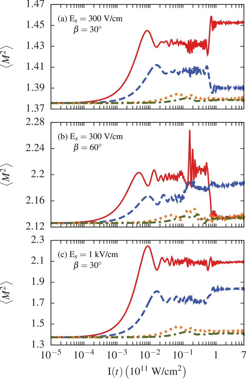
As an example, we present in Fig. 8 the time evolution of $\left\langle M^{2}\right\rangle$ for the $\left|3_{0,3}1\right>_{\text{t}}$ state in several field configurations. Before the pulse is turned on, the initial state is the adiabatic pendular level of the corresponding dc-field configuration, and, as indicated above, $\left\langle M^{2}\right\rangle$ differs from its field-free value due to the tilted electric field. As $\textup{I}(t)$ increases, $\left\langle M^{2}\right\rangle$ increases and reaches a maximum, which appears at lower intensities for longer pulses. If the pulse is short, the rotational dynamics does not adapt to the time-dependent interaction, which provokes non-adiabatic avoided crossings, and $\left\langle M^{2}\right\rangle$ does not change significantly. For longer pulses, the field-dressed dynamics is more adiabatic and larger changes on $\left\langle M^{2}\right\rangle$ are observed at moderate laser intensities, and, therefore, $\left\langle M^{2}\right\rangle$ reaches a larger value at the maximum. By increasing the dc-field strength, the Stark couplings among neighboring levels are larger provoking larger changes in $\left\langle M^{2}\right\rangle$, see Fig. 8(a) and (c). After the first maximum, $\left\langle M^{2}\right\rangle$ shows a rapid oscillatory behavior due to the presence of several avoided crossings, which are crossed diabaticaly transferring part of the population. For $\tau=10$ ns, $\text{E}_{s}=$300\text{\,}\mathrm{V}\text{/}\mathrm{cm}$$, $\beta=30^{\circ}$ and $\beta=60^{\circ}$, $\left\langle M^{2}\right\rangle$ shows a sudden change due to highly non-adiabatic avoided crossing among states with different values of $\left\langle M^{2}\right\rangle$. For $\textup{I}(t)\gtrsim${10}^{11}\text{\,}\mathrm{W}\text{/}{\mathrm{cm}}^{2}$$, $\left\langle M^{2}\right\rangle$ reaches a plateau-like behavior with small fluctuations, and, therefore, in this region the diabatic model provides a good approximation to the field-dressed dynamics.

These results show that the failure of the diabatic model mainly occurs at low or moderate laser field intensities. In this regime, the field dressed states are strongly coupled and several non-adiabatic effects take place resulting on a time-dependent wave function which is a linear combination of the eigenstates of the intantaneous field-dressed Hamiltonian. These non-adiabatic effects cannot be captured by the diabatic model, since it considers an unambiguous correspondence between eigenstates.

VI Conclusions

In this work, we have investigated the rotational dynamics of asymmetric-top molecules on a tilted-field configuration similar to those used in current mixed-field orientation experiments. By considering the benzonitrile molecule as prototype, the richness and variety of the field-dressed dynamics have been illustrated. We have addressed unique non-adiabatic effects of the tilted field configuration such as the $J$-multiplet splitting and the coupling between states with different field-free magnetic quantum numbers. By increasing the dc-field strength, the energy spacings among the states on a $J$-manifold and on the quasidegenerate pendular doublets are enhanced. Thus, the characteristic time scales of these two non-adiabatic phenomena are reduced easing the experimental requirements for an adiabatic dynamics. However, the large amount of narrow avoided crossings that emerge for moderate and strong laser intensities frustrates the hunt of an adiabatic field-dressed dynamics for rotationally excited states. As a consequence, for excited rotational states, it becomes more challenging to experimentally reach the adiabatic limit.

In this time-dependent framework, we have revisited the mixed-field orientation experiment of a state-selected molecular beam of benzonitrile Hansen et al. (2011). Our analysis includes $92.5\%$ of the molecular beam with the experimental weights, and the experimental field configuration: a weak static electric field combined with a non-resonant linearly polarized laser pulses. In this time-dependent description, the degree of orientation of the molecular ensemble is smaller than the experimentally measured Hansen et al. (2011) and similar to the orientation provided by the diabatic model Omiste et al. (2011a). By completing the molecular beam with the rest of populated states in the experiment and taking into account the volume effect, this time-dependent orientation ratio should not be significantly modified and should not become closer to the experimental one. The disagreement between the theoretical and experimental results could be due to the Coulomb explosion, and the subsequent detection of the molecular ions, and the way these processes are simulated or to the lack of adiabaticity on previous steps of the experiment, such as the state selection, which might modify the experimental weights of the rotational states in the molecular beam.

A rather natural extension of this work would be to investigate the rotational dynamics of an asymmetric-top molecule without rotational symmetry. This time-dependent study should allow us to review the conclusions of the adiabatic analysis of the 6-chloropyridazine-3-carbonitrile (CPC) in combined electric and non-resonant laser fields Hansen et al. (2013).