Electromagnetic Effects on Cracking of Anisotropic Polytropes

Abstract

In this paper, we study the electromagnetic effects on stability of spherically symmetric anisotropic fluid distribution satisfying two polytropic equations of state and construct the corresponding generalized Tolman Oppenheimer Volkoff equations. We apply perturbations on matter variables via polytropic constant as well as polytropic index and formulate the force distribution function. It is found that the compact object is stable for feasible choice of perturbed polytropic index in the presence of charge.

Keywords: Electromagnetic field; Equation of state; Cracking.
PACS: 04.40.Nr; 97.10.Cv.

1 Introduction

A stellar object is worthless if it is not stable towards perturbations in its physical variables (e.g. energy density and pressure anisotropy). The stability analysis of such objects is an interesting issue in general relativity and astrophysics. Bondi [1] was the pioneer to develop hydrostatic equilibrium equation to examine the stability of self-gravitating spheres. Herrera [2] introduced the concept of cracking as well as overturning to describe the behavior of isotropic and anisotropic matter distribution just after its deviation from equilibrium state. The cracking is observed when the radial force is positive in the inner regions but negative at outer ones while overturning is produced for the reverse situation. In general, cracking and overturning occur when total radial forces change their signs within the matter distribution.

In stellar objects, pressure anisotropy is an important matter ingredient which affects their evolution and can be produced via different physical processes such as phase transition and mixture of two fluids etc [3]. Bowers and Liang [4] studied static spherically symmetric anisotropic matter configuration and found an increase in surface redshift as well as equilibrium mass of the system. Gokhroo and Mehra [5] obtained solutions of anisotropic Einstein field equations by considering variable energy density and observed larger redshifts of spherical objects. Mak and Harko [6] discussed static anisotropic spherical stars and concluded that energy density, radial and tangential pressures are positive in the interior regions. Cosenza et al. [7] found solutions of the field equations with spherically symmetric anisotropic matter distribution.

The polytropic equation of state (EoS) has captivated the attention of many researchers to discuss the internal structure of compact objects. It is a power-law relationship between energy density and pressure defined as

$$P=k\rho^{\gamma}=k\rho^{1+\frac{1}{n}},$$

where $P,~{}\rho,~{}\gamma,~{}k$ and $n$ denote pressure, energy density, polytropic exponent, polytropic constant and polytropic index, respectively. Tooper [8] gave the idea of relativistic study of polytropes and formulated two non-linear differential equations describing the stellar structure. He found physical variables (mass, pressure and density) of polytropes using numerical technique. Herrera and Barreto [9] discussed general formalism for relativistic isotropic as well as anisotropic polytropes of spherically symmetric matter distribution and constructed the Lane-Emden equation which represents the inner structure of compact objects. Herrera et al. [10] examined the stability of spherically symmetric anisotropic conformally flat polytropes using Tolman mass and found that the considered polytropic models are stable.

Perturbation technique plays a crucial role in the stability of astrophysical objects. A star can collapse, expand, crack or overturn depending upon the nature of perturbation. Di Prisco et al. [11] discussed the cracking of spherical compact object and concluded that departure from equilibrium state leads to the cracking only for local (non-constant) anisotropic perturbation. Abreu et al. [12] examined the impact of energy density as well as local anisotropic perturbation on the stability of local and non-local anisotropic matter distributions. They found that for $P_{r}=0,~{}P_{\bot}\neq 0$, the matter configuration is always stable whereas it can experience a cracking (or overturning) when $P_{\bot}=0~{}\text{and}~{}P_{r}\neq 0$. Gonzalez et al. [13] investigated the effect of local density perturbations for isotropic as well as anisotropic spheres satisfying barotropic EoS. They obtained that isotropic configuration also presents cracking which is in contrast to the result obtained for non-local density perturbation. Recently, Herrera et al. [14] observed the cracking and overturning for anisotropic polytropes by perturbing energy density as well as local anisotropy of the system.

The study of charge in self-gravitating spherically symmetric matter distributions started with the contributions of Rosseland and Eddington [15]. Since then numerous efforts have been made to explore the effects of charge on the structure and evolution of self-gravitating systems. Bekenstein [16] discussed the gravitational collapse of charged spherically symmetric perfect fluid by introducing the idea of hydrostatic equilibrium. Bonnor [17] investigated the role of charge in the collapse of spherical dust cloud and found that it halts the process of collapse. Ray et al. [18] examined the effects of charge on compact stars and obtained $10^{10}$ coulumbs charge present in high density compact objects. Takisa and Maharaj [19] formulated exact solutions of Einstein-Maxwell field equations with polytropic EoS which can be used to model charged anisotropic compact objects. We have studied the modeling of charged conformally flat polytropic sphere and checked their viability through energy conditions [20]. Azam et al. [21] examined the occurrence of cracking in charged static spherically symmetric compact objects with quadratic EoS and concluded that stability regions increase by the increase of charge.

In this paper, we study the cracking of spherically symmetric anisotropic polytropes in the presence of charge. The format of this paper is as follows. In the next section, we study matter distribution for charged sphere and construct the generalized Tolman Oppenheimer Volkoff (TOV) equation as well as mass equation for two cases of polytropic EoS. Section 3 is devoted to observe the cracking by perturbing energy density and local anisotropy via polytropic parameters. We formulate force distribution function for each case and plot the results numerically to discuss stability of corresponding models. Finally, we conclude our results in the last section.

2 Matter Distribution and Generalized TOV Equation

We consider static spherically symmetric spacetime as follows

$$ds^{2}=-e^{\nu(r)}dt^{2}+e^{\lambda(r)}dr^{2}+r^{2}\left(d\theta^{2}+\sin^{2}\theta d\phi^{2}\right).$$ (1)

The matter distribution is considered to be anisotropic in pressure bounded by hypersurface $\Sigma$ so that $r=r_{\Sigma}=\textmd{constant}$. The energy-momentum tensor for such matter distribution is given by

$$T_{\mu\nu}=(\rho+P_{\bot})V_{\mu}V_{\nu}+P_{\bot}g_{\mu\nu}+(P_{r}-P_{\bot})S_{\mu}S_{\nu},$$ (2)

where $P_{r},~{}P_{\perp},~{}V_{\mu},~{}S_{\mu}$ are the radial pressure, tangential pressure, four-velocity and four-vector, respectively. We consider fluid to be comoving as

$$S^{\mu}=e^{-\lambda/2}\delta^{\mu}_{1},\quad V^{\mu}=e^{-\nu/2}\delta^{\mu}_{0},$$

satisfying

$$V^{\mu}V_{\mu}=-1,\quad S^{\mu}S_{\mu}=1,\quad S^{\mu}V_{\mu}=0.$$

The energy-momentum tensor for electromagnetic field is defined as

$$E_{\mu\nu}=\frac{1}{4\pi}\left(F_{\mu}~{}^{\alpha}F_{\nu\alpha}-\frac{1}{4}F^{\alpha\beta}F_{\alpha\beta}g_{\mu\nu}\right),$$ (3)

where $F_{\mu\nu}=\phi_{\nu,\mu}-\phi_{\mu,\nu}$ and $\phi_{\mu}$ are the Maxwell field tensor and four potential, respectively. The Maxwell field tensor satisfies the following field equations

$$F^{\mu\nu}_{~{}~{};\nu}={\mu}_{0}J^{\mu},\quad F_{[\mu\nu;\gamma]}=0,$$

here $\mu_{0}$ is the magnetic permeability and $J^{\mu}$ is the four current. In comoving coordinates, we have

$$\phi_{\mu}={\phi}{\delta^{0}_{\mu}},\quad J_{\mu}=\zeta V_{\mu},$$

where $\zeta=\zeta(r)$ and $\phi=\phi(r)$ represent scalar potential and charge density, respectively.

The Maxwell field equation for our spacetime yields

$$\phi^{\prime\prime}+\left(\frac{2}{r}-\frac{\nu^{\prime}}{2}-\frac{\lambda^{\prime}}{2}\right)\phi^{\prime}=4\pi\zeta e^{\frac{\nu}{2}+\lambda},$$

where prime denotes differentiation with respect to $r$. Integration of the above equation yields

$${\phi}^{\prime}=\frac{e^{\frac{\nu+\lambda}{2}}q(r)}{r^{2}}.$$

Here $q(r)=4\pi\int^{r}_{0}{\zeta}e^{\frac{\lambda}{2}}{r^{2}}dr$ indicates total charge inside the sphere. The corresponding Einstein-Maxwell field equations turn out to be

$$8{\pi}{\rho}+\frac{q^{2}}{r^{4}}=\frac{e^{-\lambda}\lambda^{\prime}}{r}-\frac{e^{-\lambda}-1}{r^{2}},$$ (4)

$$8{\pi}{P_{r}}-\frac{q^{2}}{r^{4}}=\frac{e^{-\lambda}\nu^{\prime}}{r}+\frac{e^{-\lambda}-1}{r^{2}},$$ (5)

$$8{\pi}{P_{\bot}}+\frac{q^{2}}{r^{4}}=e^{-\lambda}\left(\frac{\nu^{\prime\prime}}{2}+\frac{\nu^{\prime 2}}{4}-\frac{\nu^{\prime}\lambda^{\prime}}{4}+\frac{\nu^{\prime}}{2r}-\frac{\lambda^{\prime}}{2r}\right).$$ (6)

The corresponding Misner-Sharp mass leads to [22]

$$m(r)=\frac{r}{2}\left(1-e^{-\lambda}\right)+\frac{q^{2}}{2r}.$$ (7)

The conservation law, $T^{\mu}_{~{}\nu;\mu}+E^{\mu}_{~{}\nu;\mu}=0$, yields

$${P_{r}}^{\prime}+\frac{\nu^{\prime}}{2}\left(\rho+P_{r}\right)-\frac{2}{r}\left(P_{\bot}-P_{r}+\frac{qq^{\prime}}{8{\pi}r^{3}}\right)=0.$$ (8)

This is termed as generalized TOV equation which represents charged sphere in hydrostatic equilibrium. Using Eqs.(5) and (7), we have

$$\frac{\nu^{\prime}}{2}=\frac{4{\pi}r^{4}{P_{r}}-q^{2}+{r}{m}}{r(r^{2}-2{r}{m}+q^{2})}.$$

Consequently, Eq.(8) becomes

$${P_{r}}^{\prime}+\frac{4{\pi}r^{4}{P_{r}}-q^{2}+{r}{m}}{r^{3}-2{r^{2}}{m}+rq^{2}}(\rho+P_{r})-\frac{2\Delta}{r}-\frac{qq^{\prime}}{4{\pi}r^{4}}=0,$$ (9)

where $\Delta=P_{\bot}-P_{r}$. The polytropic EoS has two possible cases [9]. The first case gives

$$P_{r}=k\rho_{0}^{\gamma}=k\rho_{0}^{1+\frac{1}{n}},\quad\rho-\rho_{0}=nP_{r},$$ (10)

where $\rho_{0}$ is baryonic density. The polytropic EoS for the second case is

$$P_{r}=k\rho^{\gamma}=k\rho^{1+\frac{1}{n}},\quad\rho\left(1-k\rho_{0}^{\frac{1}{n}}\right)^{n}=\rho_{0},$$ (11)

where $\rho_{0}$ is replaced by $\rho$.

In the following, we evaluate generalized TOV and mass equations for the above two cases of polytropic EoS.

2.1 Case 1

We consider the first polytropic EoS (10) and construct generalized TOV equation. For this purpose, we take [10]

$$P_{rc}=\alpha\rho_{c},\quad\xi=rA,\quad A^{2}=\frac{4\pi{\rho_{c}}}{\alpha{(n+1)}},\quad\Phi_{0}^{n}=\frac{\rho_{0}}{\rho_{0c}},\quad m(r)=\frac{4{\pi}\rho_{c}\eta(\xi)}{A^{3}},$$ (12)

where subscript $c$ indicates the value at the center, $\alpha,~{}\xi,~{}\Phi_{0},~{}\eta$ are dimensionless variables and $A$ is constant. Using the variables alongwith Eq.(10) in (9), we obtain

$$\left\{\frac{1-\frac{2\eta\alpha(n+1)}{\xi}+\frac{4\pi\rho_{c}{q}^{2}}{{\xi}^{2}\alpha(n+1)}}{\alpha(n+1)\Phi_{0}+1-n\alpha}\right\}\left(\xi^{2}\frac{d\Phi_{0}}{d\xi}-2\Phi_{0}^{-n}\frac{\alpha^{4}(n+1)^{2}\xi^{3}\Delta+2\pi\alpha^{2}\rho_{c}^{2}q\frac{dq}{d\xi}}{\alpha^{5}\rho_{c}(n+1)^{3}\xi^{2}}\right)$$

$$+\alpha\xi^{3}\Phi_{0}^{n+1}+\eta-\frac{4\pi\rho_{c}q^{2}}{\xi\alpha^{2}(n+1)^{2}}=0.$$ (13)

Differentiating Eq.(7) and using (4), we obtain the mass equation as follows

$$m^{\prime}=4\pi r^{2}\rho+\frac{qq^{\prime}}{r}.$$ (14)

Using Eqs.(10) and (12) in the above equation, we have

$$\frac{d\eta}{d\xi}=\xi^{2}\Phi_{0}^{n}(1+n\alpha\Phi_{0}-n\alpha)+\frac{4\pi\rho_{c}q}{\xi\alpha^{2}(n+1)^{2}}\frac{dq}{d\xi}.$$ (15)

The coupling of generalized TOV equation (13) with mass equation (15) yields the Lane-Emden equation which provides simple models for polytropes in hydrostatic equilibrium.

2.2 Case 2

In this case, we construct TOV equation for Eq.(11) by taking

$$\Phi^{n}=\rho/\rho_{c}.$$

Consequently, Eq.(9) turns out to be

$$\left\{\frac{1-\frac{2\eta\alpha(n+1)}{\xi}+\frac{4\pi\rho_{c}{q}^{2}}{{\xi}^{2}\alpha(n+1)}}{1+\alpha\Phi}\right\}\left(\xi^{2}\frac{d\Phi}{d\xi}-2\Phi^{-n}\frac{\alpha^{4}(n+1)^{2}\xi^{3}\Delta+2\pi\alpha^{2}\rho_{c}^{2}q\frac{dq}{d\xi}}{\alpha^{5}\rho_{c}(n+1)^{3}\xi^{2}}\right)$$

$$+\alpha\xi^{3}\Phi^{n+1}+\eta-\frac{4\pi\rho_{c}q^{2}}{\xi\alpha^{2}(n+1)^{2}}=0.$$ (16)

Using Eqs.(11) and (12) in (14), it follows that

$$\frac{d\eta}{d\xi}=\xi^{2}\Phi^{n}+\frac{4\pi\rho_{c}q}{\xi\alpha^{2}(n+1)^{2}}\frac{dq}{d\xi}.$$ (17)

Again, the coupling of above two equations provides the Lane-Emden equation corresponding to this case. We see that Eqs.(13), (15) and (16), (17) form two systems of differential equations in three unknowns for case 1 and 2, respectively. In order to reduce one unknown, we consider the following EoS [14]

$$\Delta=\frac{B(4{\pi}r^{4}{P_{r}}-q^{2}+{r}{m})}{r^{2}-2{r}{m}+q^{2}}(\rho+P_{r}),$$ (18)

where $B$ is a constant.

3 Cracking of Anisotropic Polytrope

In astrophysical objects, the matter distribution may depart from equilibrium state when perturbations are introduced. We analyze the stability of polytropic compact object using the concept of cracking. For this purpose, we use Eq.(18) in (9) which yields

$$\mathcal{R}=\frac{dP_{r}}{dr}+\beta\left[\frac{4{\pi}r^{4}{P_{r}}-q^{2}+{r}{m}}{r^{3}-2{r^{2}}{m}+rq^{2}}\right](\rho+P_{r})-\frac{qq^{\prime}}{4{\pi}r^{4}},$$ (19)

here $\beta=1-2B$ and $\mathcal{R}$ represents the force distribution function. In order to observe cracking in our system, we perturb matter variables for both cases of polytropic EoS through a set of parameters ($k,\beta$) and ($n,\beta$).

3.1 Perturbations in Case 1

In this case, we construct force distribution function by perturbing the energy density and anisotropy via $k~{}\text{and}~{}\beta$ as follows

$$k\rightarrow\tilde{k}=k+\delta k,\quad\beta\rightarrow\tilde{\beta}=\beta+\delta\beta.$$

After perturbation, Eq.(10) takes the form

$$\tilde{P_{r}}=\tilde{k}\rho_{0}^{1+\frac{1}{n}}=\omega P_{r},\quad\tilde{\rho}=\rho_{0}+n\omega P_{r},$$ (20)

where $\omega=\frac{\tilde{k}}{k}$. Introducing the dimensionless variable $\hat{\tilde{\mathcal{R}}}=\frac{A}{4\pi\rho_{c}^{2}}\tilde{\mathcal{R}}$ and using the perturbed parameters alongwith Eq.(12) in (19), we have

$$\hat{\tilde{\mathcal{R}}} = \frac{\tilde{\beta}\Phi_{0}^{n}(1-n\alpha+\alpha\omega(n+1)\Phi_{0})}{\xi^{2}}\left\{\frac{\tilde{\eta}+\alpha\omega\xi^{3}\Phi_{0}^{n+1}-\frac{4\pi\rho_{c}q^{2}}{\xi\alpha^{2}(n+1)^{2}}}{1-\frac{2\tilde{\eta}\alpha(n+1)}{\xi}+\frac{4\pi\rho_{c}{q}^{2}}{{\xi}^{2}\alpha(n+1)}}\right\}$$ (21)

$$+ \omega\Phi_{0}^{n}\frac{d\Phi_{0}}{d\xi}-\frac{qq^{\prime}}{4{\pi}r^{4}}.$$

In equilibrium state, the system has no perturbation which yields $\hat{\tilde{\mathcal{R}}}(\xi,1+\delta\omega,\beta+\delta\beta,\eta+\delta\eta)=0$. Applying Taylor’s expansion, we obtain

$$\mathcal{\delta\hat{R}} = \hat{\tilde{\mathcal{R}}}(\xi,1+\delta\omega,\beta+\delta\beta,\eta+\delta\eta)=\frac{\partial\hat{\tilde{\mathcal{R}}}}{\partial\omega}|_{\omega=1,\tilde{\beta}=\beta,\tilde{\eta}=\eta}\delta\omega$$ (22)

$$+ \frac{\partial\hat{\tilde{\mathcal{R}}}}{\partial\tilde{\beta}}|_{\omega=1,\tilde{\beta}=\beta,\tilde{\eta}=\eta}\delta\beta+\frac{\partial\hat{\tilde{\mathcal{R}}}}{\partial\tilde{\eta}}|_{\omega=1,\tilde{\beta}=\beta,\tilde{\eta}=\eta}\delta\eta.$$

Using Eq.(21), we evaluate

$$\frac{\partial\hat{\tilde{\mathcal{R}}}}{\partial\omega}|_{\omega=1,\tilde{\beta}=\beta,\tilde{\eta}=\eta} = \Phi_{0}^{n}\frac{d\Phi_{0}}{d\xi}+\frac{\beta\Phi_{0}^{n+1}\alpha}{\xi^{2}\left(1-\frac{2\xi\eta\alpha(n+1)}{\xi}+\frac{4\pi\rho_{c}{q}^{2}}{{\xi}^{2}\alpha(n+1)}\right)}\left[\alpha\xi^{3}\Phi_{0}^{n}\left(2(n+1)\Phi_{0}\right.\right.$$ (23)

$$+ \left.\left.1-n\right)+(n+1)\left\{\eta-\frac{4\pi\rho_{c}q^{2}}{\xi\alpha^{2}(n+1)^{2}}\right\}\right],$$

$$\frac{\partial\hat{\tilde{\mathcal{R}}}}{\partial\tilde{\beta}}|_{\omega=1,\tilde{\beta}=\beta,\tilde{\eta}=\eta} = \frac{\Phi_{0}^{n}}{\xi^{2}}\left\{\frac{1-n\alpha+\alpha\Phi_{0}(n+1)}{1-\frac{2\eta\alpha(n+1)}{\xi}+\frac{4\pi\rho_{c}{q}^{2}}{{\xi}^{2}\alpha(n+1)}}\right\}\left[\eta+\alpha\xi^{3}\Phi_{0}^{n+1}\right.$$ (24)

$$- \left.\frac{4\pi\rho_{c}q^{2}}{\xi\alpha^{2}(n+1)^{2}}\right],$$

$$\frac{\partial\hat{\tilde{\mathcal{R}}}}{\partial\tilde{\eta}}|_{\omega=1,\tilde{\beta}=\beta,\tilde{\eta}=\eta} = \frac{\beta\Phi_{0}^{n}}{\xi^{2}}\left\{\frac{1-n\alpha+\alpha\Phi_{0}(n+1)}{\left(1-\frac{2\eta\alpha(n+1)}{\xi}+\frac{4\pi\rho_{c}{q}^{2}}{{\xi}^{2}\alpha(n+1)}\right)^{2}}\right\}\left[1+2\alpha^{2}(n+1)\xi^{2}\Phi_{0}^{n+1}\right.$$ (25)

$$- \left.\frac{4\pi\rho_{c}{q}^{2}}{{\xi}^{2}\alpha(n+1)}\right].$$

Making use of perturbed parameters in Eq.(15), we obtain

$$\tilde{\eta}=\int_{0}^{\xi}\left\{\hat{\xi}^{2}\Phi_{0}^{n}(1-n\alpha+n\alpha\omega\Phi_{0})+\frac{4\pi\rho_{c}q}{\hat{\xi}\alpha^{2}(n+1)^{2}}\frac{dq}{d\hat{\xi}}\right\}d\hat{\xi}.$$

Moreover, we have

$$\delta\eta=\frac{\partial\tilde{\eta}}{\partial\omega}|_{\omega=1}\delta\omega=n\alpha f_{1}(\xi)\delta\omega,$$ (26)

where

$$f_{1}(\xi)=\int_{0}^{\xi}\hat{\xi}^{2}\Phi_{0}^{n+1}d\hat{\xi}.$$

Substituting Eqs.(23)-(26) in (22), it follows that

$$\delta\mathcal{\hat{R}}_{1} = \Phi_{0}^{n}\left[\frac{d\Phi_{0}}{d\xi}+\frac{\alpha\beta}{\xi^{2}\left(1-\frac{2\eta\alpha(n+1)}{\xi}+\frac{4\pi\rho_{c}{q}^{2}}{{\xi}^{2}\alpha(n+1)}\right)}\left\{\alpha\xi^{3}\Phi_{0}^{n+1}\left(2(n+1)\Phi_{0}\right.\right.\right.$$

$$+ \left.\left.\left.1-n\right)+(n+1)\Phi_{0}\left\{\eta-\frac{4\pi\rho_{c}q^{2}}{\xi\alpha^{2}(n+1)^{2}}\right\}+\left(1+2\alpha^{2}(n+1)\xi^{2}\Phi_{0}^{n+1}\right.\right.\right.$$

$$- \left.\left.\left.\frac{4\pi\rho_{c}{q}^{2}}{{\xi}^{2}\alpha(n+1)}\right)\left(\frac{1-n\alpha+\alpha\Phi_{0}(n+1)}{1-\frac{2\eta\alpha(n+1)}{\xi}+\frac{4\pi\rho_{c}{q}^{2}}{{\xi}^{2}\alpha(n+1)}}\right)nf_{1}(\xi)\right\}\right]\delta\omega$$

$$+ \frac{\Phi_{0}^{n}}{\xi^{2}}\left(1-n\alpha+\alpha(n+1)\Phi_{0}\right)\left\{\frac{\eta+\alpha\xi^{3}\Phi_{0}^{n+1}-\frac{4\pi\rho_{c}q^{2}}{\xi\alpha^{2}(n+1)^{2}}}{1-\frac{2\eta\alpha(n+1)}{\xi}+\frac{4\pi\rho_{c}{q}^{2}}{{\xi}^{2}\alpha(n+1)}}\right\}\delta\beta.$$

Using the variables $x=\frac{\xi}{\bar{A}},~{}\bar{A}=r_{\Sigma}A=\xi_{\Sigma}$, the above equation yields

$$\delta\mathcal{\hat{R}}_{1} = \Phi_{0}^{n}\left[\frac{d\Phi_{0}}{\bar{A}dx}+\frac{\alpha\beta}{\bar{A}^{2}x^{2}G_{1}}\left\{\alpha\bar{A}^{3}x^{3}\Phi_{0}^{n+1}\left(2(n+1)\Phi_{0}+1-n\right)+(n+1)\Phi_{0}\left\{\eta\right.\right.\right.$$ (27)

$$- \left.\left.\left.\frac{4\pi\rho_{c}q^{2}}{\bar{A}x\alpha^{2}(n+1)^{2}}\right\}+\frac{G_{2}}{G_{1}}\left(1+2\alpha^{2}(n+1)x^{2}\bar{A}^{2}\Phi_{0}^{n+1}-\frac{4\pi\rho_{c}{q}^{2}}{x^{2}\bar{A}^{2}\alpha(n+1)}\right)\right.\right.$$

$$\times \left.\left.nf_{1}(x)\right\}\right]\delta\omega+\frac{\Phi_{0}^{n}G_{2}G_{3}}{x^{2}\bar{A}^{2}G_{1}}\delta\beta.$$

where

$$G_{1} = 1-\frac{2\alpha(n+1)\eta}{\bar{A}x}+\frac{4\pi\rho_{c}{q}^{2}}{\bar{A}^{2}x^{2}\alpha(n+1)},$$

$$G_{2} = 1-n\alpha+\alpha\Phi_{0}(n+1),$$

$$G_{3} = \eta+\alpha x^{3}\bar{A}^{3}\Phi_{0}^{n+1}-\frac{4\pi\rho_{c}q^{2}}{x\bar{A}\alpha^{2}(n+1)^{2}}.$$

In cracking, $\delta\hat{\mathcal{R}}>0$ inside the sphere while $\delta\hat{\mathcal{R}}<0$ for outer regions, so $\delta\hat{\mathcal{R}}=0$ for some value of $\xi$. This condition implies that

$$\delta\omega=-\frac{\delta\beta}{\Gamma},$$

where $\Gamma=\frac{\frac{\partial\hat{\tilde{\mathcal{R}}}}{\partial\omega}+\frac{\partial\hat{\tilde{\mathcal{R}}}}{\partial\tilde{\eta}}f_{1}(\xi)}{\frac{\partial\hat{\tilde{\mathcal{R}}}}{\partial\tilde{\beta}}}|_{\omega=1,\tilde{\beta}=\beta,\tilde{\eta}=\eta}$.

We study a phenomenon of cracking by perturbing energy density and anisotropy via parameters $n~{}\text{and}~{}\beta$ as follows

$$n\rightarrow\tilde{n}=n+\delta n,\quad\beta\rightarrow\tilde{\beta}=\beta+\delta\beta.$$

Equation (19) in terms of perturbed parameters can be written as

$$\hat{\tilde{\mathcal{R}}} = \Phi_{0}^{\tilde{n}}\frac{d\Phi_{0}}{d\xi}+\frac{\tilde{\beta}\Phi_{0}^{\tilde{n}}\left(1-\tilde{n}\alpha+\alpha(\tilde{n}+1)\Phi_{0}\right)}{\xi^{2}}\left\{\frac{\tilde{\eta}+\alpha\xi^{3}\Phi_{0}^{\tilde{n}+1}-\frac{4\pi\rho_{c}q^{2}}{\xi\alpha^{2}(\tilde{n}+1)^{2}}}{1-\frac{2\tilde{\eta}\alpha(\tilde{n}+1)}{\xi}+\frac{4\pi\rho_{c}{q}^{2}}{{\xi}^{2}\alpha(\tilde{n}+1)}}\right\}$$ (28)

$$- \frac{qq^{\prime}}{4{\pi}r^{4}}.$$

In this scheme, Taylor’s expansion yields

$$\delta\hat{\mathcal{R}}=\frac{\partial\hat{\tilde{\mathcal{R}}}}{\partial\tilde{n}}|_{\tilde{n}=n,\tilde{\beta}=\beta,\tilde{\eta}=\eta}\delta n+\frac{\partial\hat{\tilde{\mathcal{R}}}}{\partial\tilde{\eta}}|_{\tilde{n}=n,\tilde{\beta}=\beta,\tilde{\eta}=\eta}\delta\eta+\frac{\partial\hat{\tilde{\mathcal{R}}}}{\partial\tilde{\beta}}|_{\tilde{n}=n,\tilde{\beta}=\beta,\tilde{\eta}=\eta}\delta\beta.$$

Making use of Eq.(28), the above equation turns out to be

$$\delta\mathcal{\hat{R}}_{2} = \Phi_{0}^{n}\left[\frac{\ln\Phi_{0}}{\bar{A}}\frac{d\Phi_{0}}{dx}+\frac{\beta}{\bar{A}^{2}x^{2}G_{1}}\left\{\ln\Phi_{0}G_{2}G_{3}+\alpha(\Phi_{0}-1)G_{3}+G_{2}\left(\alpha A^{3}x^{3}\right.\right.\right.$$ (29)

$$\times \left.\left.\left.\Phi_{0}^{n+1}\ln\Phi_{0}+\frac{8\pi\rho_{c}q^{2}}{\bar{A}x\alpha^{2}(n+1)^{3}}\right)+\frac{G_{2}G_{3}}{G_{1}}\left(\frac{2\eta\alpha}{\bar{A}x}+\frac{4\pi\rho_{c}q^{2}}{\bar{A}^{2}x^{2}\alpha(n+1)^{2}}\right)\right.\right.$$

$$+ \left.\left.\frac{G_{2}}{G_{1}}\left(G_{1}+\frac{2\alpha(n+1)}{\bar{A}x}G_{3}\right)f_{2}(x)\right\}\right]\delta n+\frac{\Phi_{0}^{n}}{\bar{A}^{2}x^{2}}\frac{G_{2}G_{3}}{G_{1}}\delta\beta,$$

where

$$f_{2}(x)=\int_{0}^{x}\bar{A}^{3}\hat{x}^{2}\Phi_{0}^{n}\left\{\alpha(\Phi_{0}^{1-n}-1)+(1-n\alpha)\ln\Phi_{0}\right\}d\hat{x}.$$ (30)

Again, for cracking to occur, $\delta\hat{\mathcal{R}}=0$ implying that

$$\delta n=-\frac{\delta\beta}{\Gamma},$$

where $\Gamma=\frac{\frac{\partial\hat{\tilde{\mathcal{R}}}}{\partial\tilde{n}}+\frac{\partial\hat{\tilde{\mathcal{R}}}}{\partial\tilde{\eta}}f_{2}(\xi)}{\frac{\partial\hat{\tilde{\mathcal{R}}}}{\partial\tilde{\beta}}}|_{\tilde{n}=n,\tilde{\beta}=\beta,\tilde{\eta}=\eta}$.

3.2 Perturbations in Case 2

Here, we develop force distribution function for the second kind of polytropic EoS using perturbed parameters ($k,\beta$). After perturbation, the energy density takes the form

$$\tilde{\rho}=\rho+\delta\rho=\rho+\frac{\partial\tilde{\rho}}{\partial\omega}|_{\omega=1},$$

which yields

$$\tilde{\rho}=\rho+nP_{r}(1-\omega),$$

where we have used $\omega=1+\delta\omega$. Using perturbed parameters in Eq.(19), we have

$$\hat{\tilde{\mathcal{R}}} = \omega\Phi^{n}\frac{d\Phi}{d\xi}+\frac{\tilde{\beta}\Phi^{n}\left[1+\alpha\Phi\{n+\omega(1-n)\}\right]}{\xi^{2}\left(1-\frac{2\eta\alpha(n+1)}{\xi}+\frac{4\pi\rho_{c}{q}^{2}}{{\xi}^{2}\alpha(n+1)}\right)}\left\{\tilde{\eta}+\alpha\omega\xi^{3}\Phi^{n+1}\right.$$

$$- \left.\frac{4\pi\rho_{c}q^{2}}{\xi\alpha^{2}(n+1)^{2}}\right\}-\frac{qq^{\prime}}{4{\pi}r^{4}}.$$

Applying Taylor’s expansion on the above equation, it follows that

$$\delta\mathcal{\hat{R}}_{3} = \Phi^{n}\left[\frac{d\Phi}{\bar{A}dx}+\frac{\alpha\beta}{\bar{A}^{2}x^{2}G_{1}}\left\{\Phi(1-n)\left(\eta-\frac{4\pi\rho_{c}q^{2}}{x\bar{A}\alpha^{2}(n+1)^{2}}\right)+x^{3}\bar{A}^{3}\alpha(1-n)\right.\right.$$ (31)

$$\times \left.\left.\Phi^{n+2}-n(1+\alpha\Phi)\left(\frac{1+2\alpha^{2}\bar{A}^{2}x^{2}(n+1)\Phi^{n+1}}{G_{1}}\right)f_{3}(x)\right\}\right]\delta\omega$$

$$+ \frac{\Phi^{n}}{x^{2}\bar{A}^{2}}\left(1+\alpha\Phi\right)\frac{G_{3}}{G_{1}}\delta\beta,$$

where $f_{3}(x)=\int_{0}^{x}\bar{A}^{3}\hat{x}^{2}\Phi^{n+1}d\hat{x}$. Similarly, perturbation of $n~{}\text{and}~{}\beta$ leads to

$$\delta\mathcal{\hat{R}}_{4} = \Phi^{n}\left[\frac{\ln\Phi}{\bar{A}}\frac{d\Phi}{dx}+\frac{\beta}{\bar{A}^{2}x^{2}}\left\{\frac{\ln\Phi G_{4}G_{5}}{G_{1}}+\frac{G_{5}}{G_{1}}\left(\alpha A^{3}x^{3}\Phi^{n+1}\ln\Phi\right.\right.\right.$$ (32)

$$+ \left.\left.\left.\frac{8\pi\rho_{c}q^{2}}{\bar{A}x\alpha^{2}(n+1)^{3}}\right)-\frac{G_{4}G_{5}}{G_{1}^{2}}\left(-\frac{2\eta\alpha}{\bar{A}x}-\frac{4\pi\rho_{c}q^{2}}{\bar{A}^{2}x^{2}\alpha(n+1)^{2}}\right)\right.\right.$$

$$+ \left.\left.\frac{G_{5}}{G_{1}^{2}}\left(G_{1}+\frac{2\alpha(n+1)}{\bar{A}x}\bar{G}_{4}\right)f_{2}(x)\right\}\right]\delta n+\frac{\Phi^{n}}{\bar{A}^{2}x^{2}}\frac{G_{4}G_{5}}{G_{1}}\delta\beta,$$

where

$$G_{4} = \eta+\alpha x^{3}\bar{A}^{3}\Phi^{n+1}-\frac{4\pi\rho_{c}q^{2}}{x\bar{A}\alpha^{2}(n+1)^{2}},\quad G_{5}=1+\alpha\Phi,$$

$$f_{4}(x) = \int_{0}^{x}\bar{A}^{3}\hat{x}^{2}\Phi^{n}\ln\Phi d\hat{x}.$$

Now we analyze the occurrence of cracking in the polytropic models through numerical method. We examine the charged compact models for both cases of polytropic EoS with perturbations through ($k,\beta$) and ($n,\beta$). Firstly, we evaluate $\Phi_{0}~{},\Phi~{}\text{and}~{}\eta$ for both cases by integrating Eqs.(13), (15), (16) and (17) with boundary conditions [10]

$$\eta(0)=0,\quad\Phi_{0}(0)=1,\quad\Phi_{0}(\xi_{\Sigma})=0,\quad\Phi(0)=1,\quad\Phi(\xi_{\Sigma})=0,$$

and use these results to plot force distribution functions. The graphical behavior of force distribution function for the case 1 is shown in Figure 1. The left graph shows the behavior of $\delta\mathcal{\hat{R}}_{1}$ indicating that for all considered values of $q$, it is positive in the inner regions and becomes negative for the outer ones thus ensuring the occurrence of strongest cracking in the corresponding model. The right graph is plotted for $\delta\mathcal{\hat{R}}_{2}$ which shows that there is neither cracking nor overturning for all values of $q$. Thus, the presence of charge in polytropes leads to stable models.

For the case 2, the plots of force function in Eqs.(31) and (32) for different values of the parameters are shown in Figure 2. The left graph is plotted for $\delta\mathcal{\hat{R}}_{3}$ which indicates stable behavior for $q=0.2M_{0}$ while the strongest overturning appears for other two values of $q$. The graphical analysis of $\delta\mathcal{\hat{R}}_{4}$ for different values of charge shows stable configuration as shown in Figures 2 (right) and 3. It is observed that within uncharged matter distribution both cracking and overturning appear. However, the inclusion of charge in matter configurations leads to stability of spherically symmetric polytrope.

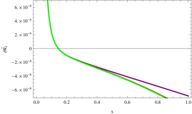
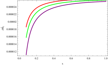
Figure 1: Left plot for $\delta\hat{\mathcal{R}_{1}}$ versus $x$ with $n=1,\alpha=0.85,\beta=1.5,\Gamma=1.6,q=0.2M_{0}$ (purple), $q=0.4M_{0}$ (red), $q=0.64M_{0}$ (green). Right plot for $\delta\hat{\mathcal{R}_{2}}$ versus $x$ with $n=1.5,\alpha=0.90,\beta=0.5,\Gamma=1.4,q=0.2M_{0}$ (purple), $q=0.4M_{0}$ (red), $q=0.64M_{0}$ (green).

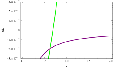
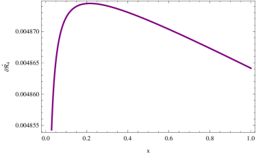
Figure 2: Left plot for $\delta\hat{\mathcal{R}_{3}}$ versus $x$ with $n=0.5,\alpha=0.98,\beta=1.5,\Gamma=0.6,q=0.2M_{0}$ (purple), $q=0.4M_{0}$ (red), $q=0.64M_{0}$ (green). Right plot for $\delta\hat{\mathcal{R}_{4}}$ versus $x$ with $n=1.5,\alpha=0.7,\beta=1.5,\Gamma=-0.5,q=0.2M_{0}$.

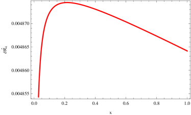
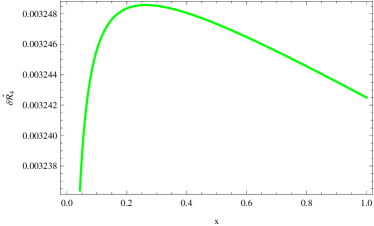
Figure 3: Plot for $\delta\hat{\mathcal{R}_{4}}$ versus $x$ with $n=1.5,\alpha=0.7,\beta=1.5,\Gamma=-0.5$. Left plot for $q=0.4M_{0}$. Right plot for $q=0.64M_{0}$.

4 Concluding Remarks

The stability analysis of stellar objects is an interesting area of research. The concept of cracking refers to the appearance of total radial forces of different signs within the matter distribution. If there is no cracking (or overturning) within a particular configuration, then the system is not completely stable since other types of perturbation can lead to its cracking, overturning, expansion or collapse. We have considered spherically symmetric star with charged anisotropic matter distribution satisfying polytropic EoS and constructed the corresponding Einstein-Maxwell equations. We have considered two cases of polytropic EoS and formulated TOV as well as mass equations in terms of dimensionless variables for each case. The coupling of these two equations represent charged polytrope in hydrostatic equilibrium.

In order to observe cracking, perturbation is a necessary ingredient to take out system from equilibrium state. We have perturbed energy density and pressure anisotropy of a system in two ways. Firstly, we have introduced perturbations through parameters ($k,\beta$) and constructed the force distribution function $(\delta\mathcal{\hat{R}}_{1})$ in terms of perturbed parameters describing total radial forces present in a system. The graphical analysis of $\delta\mathcal{\hat{R}}_{1}$ indicates the appearance of cracking for all choices of parameters thus leading to unstable configurations for this case. Secondly, we have used ($n,\beta$) as perturbation parameters and constructed $\delta\mathcal{\hat{R}}_{2}$. It is found that the resulting models are stable towards perturbations.

We have followed the same procedure for the case 2 of polytropic EoS and constructed $\delta\mathcal{\hat{R}}_{3}~{}\text{as well as}~{}\delta\mathcal{\hat{R}}_{4}$. It is found that polytropic models are unstable for perturbation in ($k,\beta$), while the perturbation of ($n,\beta$) leads to stable matter configuration representing relativistic polytrope. The stability of compact objects depends upon the choice of EoS. It was found that spherically symmetric charged compact objects with quadratic EoS [21] lead to stable models while the linear EoS [23] provides unstable configurations. For uncharged spherical anisotropic polytropes, both cracking and overturning appear for a wide range of parameters under ($k,\beta$) as well as ($n,\beta$) perturbations [14]. We have observed that charged matter distribution leads to stable configurations for ($n,\beta$) perturbation while polytropic models remain unstable by perturbing ($k,\beta$). We conclude that that the inclusion of charge in anisotropic fluid distribution has a dominant effect on polytropes which leads to stable models.

References

• [1] Bondi, H.: Proc. Roy. Soc. Lond. A 282(1964)303.
• [2] Herrera, L.: Phys. Lett. A 165(1992)206.
• [3] Sawyer, R.F.: Phys. Rev. Lett. 29(1972)823; Letelier, P.S.: Phys. Rev. D 22(1980)807; Herrera, L. and Santos, N.O.: Astrophys. J. 438(1995)308; Phys. Rep. 286(1997)53.
• [4] Bowers, R.L. and Liang, E.P.T.: Astrophys. J. 188(1974)657.
• [5] Gokhroo, M.K. and Mehra, A.L.: Gen. Relativ. Gravit. 26(1994)75.
• [6] Mak, M.K. and Harko, T.: Proc. Roy. Soc. Lond. A 459(2003)393.
• [7] Cosenza, M., Herrera, L., Esculpi, M. and Witten, L.: J. Math. Phys. 22(1981)118.
• [8] Tooper, R.: Astrophys. J. 140(1964)434.
• [9] Herrera, L. and Barreto, W.: Phys. Rev. D 88(2013)084022.
• [10] Herrera, L., Di Prisco, A., Barreto, W. and Ospino, J.: Gen. Relativ. Gravit. 46(2014)1827.
• [11] Di Prisco, A., Herrera, L. and Varela, V.: Gen. Relativ. Gravit. 29(1997)1239.
• [12] Abreu, H., Hern$\acute{a}$ndez, H. and N$\acute{u}\tilde{n}$ez, L.A.: Class. Quantum Grav. 24(2007)4631.
• [13] Gonzalez, G.A., Navarro, A. and N$\acute{u}\tilde{n}$ez , L.A.: J. Phys. Conf. Ser. 600(2015)012014.
• [14] Herrera, L., Fuenmayor, E. and Le$\acute{o}$n, P.: Phys. Rev. D 93(2016)024047.
• [15] Rosseland, S. and Eddington, A.S.: Mon. Not. R. Astron. Soc. 84(1924)720.
• [16] Bekenstein, J.D.: Phys. Rev. D 4(1960)2185.
• [17] Bonnor, W.B.: Mon. Not. R. Astron. Soc. 129(1964)443.
• [18] Ray, S., Malheiro, M., Lemos, J.P.S. and Zanchin, V.T.: Braz. J. Phys. 34(2004)310.
• [19] Takisa, P.M. and Maharaj, S.D.: Gen. Relativ. Gravit. 45(2013)1951.
• [20] Sharif, M. and Sadiq, S.: Can. J. Phys. 93(2015)1420.
• [21] Azam, M., Mardan, S.A. and Rehman, M.A.: Adv. High Energy Phys. 2015(2015)865086.
• [22] Misner, C.W. and Sharp, D.H.: Phys. Rev. 136(1964)B571.
• [23] Azam, M., Mardan, S.A. and Rehman, M.A.: Astrophys. Space Sci. 359(2015)14.