A new algorithm for computing branching rules and Clebsch–Gordan coefficients of unitary representations of compact groups 

Abstract

A numerical algorithm that computes the decomposition of any finite-dimensional unitary reducible representation of a compact Lie group is presented. The algorithm, which does not rely on an algebraic insight on the group structure, is inspired by quantum mechanical notions. After generating two adapted states (these objects will be conveniently defined in Def. II.1) and after appropriate algebraic manipulations, the algorithm returns the block matrix structure of the representation in terms of its irreducible components. It also provides an adapted orthonormal basis. The algorithm can be used to compute the Clebsch–Gordan coefficients of the tensor product of irreducible representations of a given compact Lie group. The performance of the algorithm is tested on various examples: the decomposition of the regular representation of two finite groups and the computation of Clebsch–Gordan coefficients of two examples of tensor products of representations of $SU(2)$.

I Introduction

The algorithm presented in this paper solves the problem of numerically determining the decomposition of a finite-dimensional irreducible unitary linear representation (‘irrep’ in what follows) of a compact group $G$ with respect to the unitary irreducible representations (irreps) of a given subgroup $H\subset G$.

More precisely, let $G$ be a compact Lie group and $(\mathcal{H},U)$ a finite-dimensional irreducible unitary representation of it, i.e., $U\colon G\to U(\mathcal{H})$ is a group homomorphism that satisfies the following three conditions:

$$\begin{array}[]{c}\vspace{-1cm}\phantom{a}\\ (C.1)\\ \vspace{-1cm}\phantom{a}\end{array} \hskip 65.44142pt\begin{array}[]{c}\vspace{-1cm}\phantom{a}\\ U(g_{1}g_{2})=U(g_{1})U(g_{2}),\qquad\text{for all $g_{1},g_{2}\in G$.}\\ \vspace{-1cm}\phantom{a}\end{array}$$

$$\begin{array}[]{c}\vspace{-1cm}\phantom{a}\\ (C.2)\\ \vspace{-1cm}\phantom{a}\end{array} \hskip 65.44142pt\begin{array}[]{c}\vspace{-1cm}\phantom{a}\\ U(e)=\mathds{1}\,.\\ \vspace{-1cm}\phantom{a}\end{array}$$

$$\begin{array}[]{c}\vspace{-1cm}\phantom{a}\\ (C.3)\\ \vspace{-1cm}\phantom{a}\end{array} \hskip 65.44142pt\begin{array}[]{c}\vspace{-1cm}\phantom{a}\\ U(g^{-1})=U(g)^{-1}=U(g)^{\dagger},\qquad\text{for all $g\in G$.}\\ \vspace{-1cm}\phantom{a}\end{array}$$

Here, $\mathcal{H}$ is a complex Hilbert space with inner product $\langle\cdot,\cdot\rangle$, $U(\mathcal{H})$ is the group of unitary operators on $\mathcal{H}$ and ^† stands for the adjoint.

Conditions $(C.1)$ – $(C.3)$ above define a unitary representation $(\mathcal{H},U)$ of the group $G$. The representation is said to be irreducible if there are no proper invariant subspaces of $\mathcal{H}$, i.e., if any linear subspace $W\subset\mathcal{H}$ is such that $U(g)W\subset W$ for all $g\in G$, then $W$ is either $\{\mathbf{0}\}$ or $\mathcal{H}$. Since the group $G$ is compact, any irreducible representation of $G$ will be finite-dimensional with dimension say $n$ ($n=\dim\mathcal{H}$).

Consider a closed subgroup $H\subset G$. The restriction of $U$ to $H$ will define a unitary representation of $H$ which is reducible in general, that is, it will possess invariant subspaces $\mathcal{L}^{\alpha}$ such that $U(h)\mathcal{L}^{\alpha}\subset\mathcal{L}^{\alpha}$ for all $h\in H$. If we denote by $\widehat{H}$ the family of equivalence classes of irreps of $H$ (recall that two unitary representations of $H$, $V\colon H\to U(E)$ and $V^{\prime}\colon H\to U(E^{\prime})$, are equivalent if there exists a unitary map $T\colon E\to\displaystyle{E^{\prime}}$ such that $\displaystyle{V}^{\prime}(h)\circ T=T\circ V(h)$ for all $h\in H$), then:

$$\mathcal{H}=\bigoplus_{\alpha\in\widehat{H}}\mathcal{L}^{\alpha}\,,\qquad\mathcal{L}^{\alpha}=c_{\alpha}\mathcal{H}^{\alpha}\,=\bigoplus_{a=1}^{c_{\alpha}}\mathcal{H}^{\alpha}\,,$$ (1)

where $c_{\alpha}$ are non-negative integers, $\{\alpha\}$ denotes a subset in the class of irreps of the group $H$ (each $\alpha$ denotes a finite-dimensional irrep of $H$ formed by the pair $(\mathcal{H}^{\alpha},U^{\alpha})$) and $c_{\alpha}\mathcal{H}^{\alpha}$ denotes the direct sum of the linear space $\mathcal{H}^{\alpha}$ with itself $c_{\alpha}$ times. Thus, the family of non-negative integer numbers $c_{\alpha}$ denotes the multiplicity of the irreps $(\mathcal{H}^{\alpha},U^{\alpha})$ in $(\mathcal{H},U)$. The numbers $c_{\alpha}$ satisfy $n=\sum_{\alpha}c_{\alpha}n_{\alpha}$ where $n_{\alpha}=\dim\mathcal{H}^{\alpha}$ and the invariant subspaces $\mathcal{L}^{\alpha}$ have dimension $c_{\alpha}n_{\alpha}$. Notice that the unitary operator $U(h)$ will have the corresponding block structure:

$$U(h)=\bigoplus_{\alpha\in\widehat{H}}c_{\alpha}U^{\alpha}(h)\,,\qquad\forall h\in H\,,$$ (2)

where $\displaystyle{U}^{\alpha}(h)=U(h)\mid_{\mathcal{H}^{\alpha}}$.

The problem of determining an orthonormal basis of $\mathcal{H}$ adapted to the decomposition (1) will be called the Clebsch–Gordan problem of $(\mathcal{H},U)$ with respect to the subgroup $H$. To be more precise, the Clebsch–Gordan problem of the representation $U$ of $G$ in $\mathcal{H}$ with respect to the subgroup $H$ consists in finding an orthonormal basis $\{u_{a,k}^{\alpha}\mid\alpha\in\widehat{H},a=1,\ldots,c_{\alpha},\,k=1,\ldots,n_{\alpha}\}$ of $\mathcal{H}$ such that each family $\{u_{a,k}^{\alpha}\}_{k=1}^{n_{\alpha}}$, for a given $\alpha$, defines an orthonormal basis of $\mathcal{H}^{\alpha}$. Thus, given an arbitrary orthonormal basis $\{u_{l}\}_{l=1}^{n}\subset\mathcal{H}$, we can compute the $n\times n$ unitary matrix $C$ with entries $C_{a,kl}^{\alpha}$ such that

$$u_{l}=\sum_{\alpha,a,k}C_{a,kl}^{\alpha}u_{a,k}^{\alpha}\,,\qquad\alpha\in\widehat{H},\quad a=1,\ldots,c_{\alpha},\quad k=1,\ldots,n_{\alpha},\quad l=1,\ldots,n\,.$$ (3)

The coefficients $C_{a,kl}^{\alpha}$ of the matrix $C$ are usually expressed as the symbol $(l\mid\alpha,a,k)$ and are called the Clebsch–Gordan coefficients of the decomposition.

The original Clebsch–Gordan problem has its origin in the composition of two quantum systems possessing the same symmetry group: let $\mathcal{H}_{A}$ and $\mathcal{H}_{B}$ denote Hilbert spaces corresponding respectively to two quantum systems $A$ and $B$, which support respective irreps $U_{A}$ and $U_{B}$ of a Lie group $G$. Then, the composite system, whose Hilbert space is $\mathcal{H}=\mathcal{H}_{A}\widehat{\otimes}\mathcal{H}_{B}$, supports an irrep of the product group $G\times G$. The interaction between both systems gives rise to a only remaining subgroup $H\subset G\times G$ as a symmetry group of the composite system (in many instances, it is just $H=G$ with $G$ considered as the diagonal subgroup $G\subset G\times G$ of the product group). The tensor product representation $U_{A}\otimes U_{B}$ will no longer be irreducible with respect to the subgroup $H\subset G\times G$ and we will be compelled to consider its decomposition into irrep components.

A considerable effort has been put in computing the Clebsch–Gordan matrix for various situations of physical interest. For instance, the groups $SU(N)$ have been widely discussed (see [Al10, ], [Gl07, ] and references therein) since when considering the groups $SU(3)$ and $SU(2)$, the Clebsch–Gordan matrix provides the multiplet structure and the spin components of a composite system of particles (see [Ro97, ], [Wi94, ]). However, all these results depend critically on the algebraic structure of the underlying group $G$ (and the subgroup $H$) and no algorithm was known so far to efficiently compute the Clebsch–Gordan matrix for a general subgroup $H\subset G$ of an arbitrary compact group $G$.

On the other hand, the problem of determining the decomposition of an irreducible representation with respect to a given subgroup has not been addressed from a numerical point of view. The multiplicity of a given irreducible representation $(\mathcal{H}^{\alpha},U^{\alpha})$ of the compact group $G$ in the finite-dimensional representation $(\mathcal{H},U)$ is given by the inner product

$$c_{\alpha}=\frac{1}{|G|}\langle\chi^{\alpha},\chi\rangle\,,$$

where $\chi^{\alpha}(g)=\mathrm{Tr}(U^{\alpha}(g))$ and $\chi(g)=\mathrm{Tr}(U(g))$, $g\in G$, denote the characters of the corresponding representations, $|G|$ is the order of the group $G$ and $\langle\cdot,\cdot\rangle$ stands for the standard inner product of central functions with respect to the (left-invariant) Haar measure on $G$. Hence, if the characters $\chi^{\alpha}$ of the irreducible representations of $G$ are known, the computation of the multiplicities becomes, in principle, a simple task. Moreover, given the characters $\chi^{\alpha}$ of the irreducible representations, the projector method would allow us to explicitly construct the Clebsch–Gordan matrix [Tu85, , Ch. 4]. However, if the irreducible representations of $H$ are not known in advance (or are not explicitly described), there is no an easy way of determining the multiplicities $c_{\alpha}$.

Again, at least in principle, the computation of the irreducible representations of a finite group could be achieved by constructing its character table, i.e., a $c\times c$ unitary matrix where $c$ is the number of conjugacy classes of the group, but again, there is no a general-purpose numerical algorithm for doing that.

Recent developments in quantum group tomography require dealing with a broad family of representations of a large class of groups, compact or not, and their subgroups (see [Ib09, ] and references therein for a recent overview on the subject). Quantum tomography allows to extend ideas from standard classical tomography to analyze states of quantum systems. One implementation of quantum tomography is quantum group tomography. Quantum group tomography is based on quantum systems supporting representations of groups. Such representations make it possible to construct the corresponding tomograms for given quantum states [Ar05, , Ib11, , LY15, ]. Hence it is becoming increasingly relevant to have new tools to efficiently handle group representations and their decompositions.

It turns out that it is precisely the ideas and methods from quantum tomography which provide the clue for the numerical algorithm presented in this work. More explicitly, mixed quantum states, i.e., density matrices adapted to a given representation, will be used to compute the Clebsch–Gordan matrix. Section II will be devoted to introduce the problem we want to solve. Section III presents several results which will help us to show the correctness of the algorithm. The details of the numerical algorithm are contained in Section IV, while Section V covers various examples and applications of the algorithm, among them, the decomposition of regular representations of any finite group and the decomposition of multipartite systems of spin particles.

It is remarkable that the algorithm proposed here does not require an a priori knowledge of the irreducible representations of the groups and the irreducible representations themselves are returned as outcomes of the algorithm. This makes the proposed algorithm an effective tool for computing the irreducible representations, in principle, for any finite or compact group. For the sake of clarity, most of the analysis will be done in the case of finite groups, however it should be noted that all statements and proofs can be easily lifted to compact groups by replacing finite sums over group elements by the corresponding integrals over the group with respect to the normalized Haar measure on it. Some additional remarks and outcomes will be discussed at the end in Section VI. A final Appendix contains numerical results for the examples addressed in Section V.

II The setting of the problem

Let $G$ be a finite group of order $|G|=s$ and let $H\subset G$ be a subgroup of $G$, not necessarily normal, of order $|H|=r$. We label the elements of $G$ as  $G=\{e=h_{0},g_{1}=h_{1},\ldots,g_{r-1}=h_{r-1},g_{r},\ldots,g_{s-1}\}$, where the first $r$ elements correspond to the elements of the subgroup $H$, i.e., $H=\{e=h_{0},h_{1},\ldots,h_{r-1}\}$. In what follows, a generic element in the group $G$ will be simply denoted by $g\in G$ unless some specific indexing is required.

Let $U$ be a unitary irreducible representation of $G$ on the finite-dimensional Hilbert space $\mathcal{H}$, $n=\dim\mathcal{H}$, and let $e_{i}$, $i=1,\ldots,n$, be any given orthonormal basis of $\mathcal{H}$. We denote by

$$D(g)=\left[D_{ij}(g)\right]_{i,j=1}^{n}$$ (4)

the unitary matrix associated with $U(g)$, $g\in G$, in the chosen basis, i.e.,

$$D_{ij}(g)=\langle e_{i},U(g)e_{j}\rangle\,$$ (5)

for every $i,j=1,\ldots,n$. The restriction of the representation $U$ to the subgroup $H$, sometimes denoted by $U\!\!\downarrow\!\!H$ and called the subduced representation of $U$ to $H$, will be, in general, reducible even if $U$ is irreducible. Notice that the unitary matrix associated with $U\!\downarrow\!H(h)$, $h\in H$, is just a submatrix of $D_{ij}(h)$ obtained by restricting ourselves to the elements of the subgroup $H$.

A mixed state on $\mathcal{H}$, also called a density matrix, is a $n\times n$ normalized Hermitian positive semidefinite matrix $\rho$, i.e.,

$$\rho=\rho^{\dagger}\,,\qquad\rho\geq 0\,,\qquad\mathrm{Tr}(\rho)=1\,.$$ (6)

If the unitary representation $U$ of $G$ is irreducible, then any state $\rho$ can be written as:

$$\rho=\frac{n}{|G|}\sum_{g\in G}\mathrm{Tr}\left(\rho\,D(g)^{\dagger}\right)\,D(g)\,.$$ (7)

To prove this formula one may use Schur’s orthogonality relations:

$$\sum_{g\in G}D^{\alpha}_{mn}(g)^{*}D^{\beta}_{pq}(g)=\frac{|G|}{n_{\alpha}}\delta_{\alpha\beta}\delta_{mp}\delta_{nq}\,,$$ (8)

where $*$ stands for the complex conjugate and elements $D^{\alpha}_{mn}(g)$ and $D^{\beta}_{mn}(g)$ denote, respectively, the entries of the unitary matrices $D^{\alpha}(g)$ and $D^{\beta}(g)$ associated with the irreducible representations $(\mathcal{H}^{\alpha},U^{\alpha})$ and $(\mathcal{H}^{\beta},U^{\beta})$ of the group $G$ with respect to given arbitrary orthonormal bases in $\mathcal{H}^{\alpha}$ and $\mathcal{H}^{\beta}$.

Let us now consider a state $\rho$ satisfying the orthogonality relations

$$\mathrm{Tr}(\rho\,D(g_{k}))=0\,,\qquad k=r,\ldots,s-1\,.$$ (9)

Clearly, because of eq. (7), such a state verifies

$$\rho=\frac{n}{|G|}\sum_{h\in H}\mathrm{Tr}\left(\rho\,D(h)^{\dagger}\right)\,D(h)\,.$$ (10)

Definition II.1.

A state $\rho$ in the Hilbert space $\mathcal{H}$ supporting an irrep $U$ of the group $G$ is said to be adapted to a closed subgroup $H$ if $\mathrm{Tr}(\rho\,D(g))=0$ for $g\notin H$.

In other words, a state $\rho$ adapted to the subgroup $H$ of the finite group $G$ must be of the form:

$$\rho=\frac{n}{|G|}\sum_{i=0}^{r-1}\mathrm{Tr}\left(\rho\,D(h_{i})^{\dagger}\right)\,D(h_{i})\,,$$

even if the subduced representation $U\!\downarrow\!H$ is reducible.

In view of the prominent role they will play in the algorithm, let us now discuss briefly the role of the inner products $\mathrm{Tr}(\rho A)$ in the realm of quantum theory: given a linear operator $A$ on $\mathcal{H}$ and a state $\rho$, the number $\mathrm{Tr}(\rho A)$ is called the expected value of the operator $A$ in the state $\rho$ and it is denoted consequently as $\langle A\rangle_{\rho}$. If the operator $A$ is self-adjoint, the expected value $\langle A\rangle_{\rho}$ is a real number and it truly represents the expected value of measuring the observable described by the operator $A$ on a quantum system in the state $\rho$.

In the language of quantum tomography, the group function $\chi_{\rho}\,\colon G\to\mathbb{C}$ defined by the coefficients in the expansion written in eq. (7),

$$\chi_{\rho}(g)=\mathrm{Tr}(\rho\,D(g))\,,\qquad g\in G\,,$$ (11)

is called the characteristic function of the state $\rho$ associated with the representation $(\mathcal{H},U)$ or, depending on the emphasis, the smeared character of the representation $U$ with respect to the state $\rho$ (see [LY15, ]). One can easily check that the characteristic function $\chi_{\rho}$ is always positive semidefinite, i.e.,

$$\sum_{j,k=1}^{N}\xi_{j}^{*}\xi_{k}\,\chi_{\rho}(g_{j}^{-1}g_{k})\geq 0\,,$$ (12)

for all $N\in\mathbb{N}$, $\xi_{j},\xi_{k}\in\mathbb{C}$ and $g_{j},g_{k}\in G$.

Notice that if the state is $\rho=\frac{1}{n}\mathds{1}$, the characteristic function $\chi_{\rho}$ is the standard character $\chi(g)$ of the representation $D(g)$ divided by $n$. Moreover, if the representation $D(g)$ is the trivial one, then $\chi_{\rho}(g)=1$ for all $g\in G$.

Definition II.2.

Let $G$ be a group, $(\mathcal{H},U)$ an irreducible unitary representation of $G$ and $H$ a closed subgroup of $G$. The Clebsch–Gordan matrix associated with $G$, $H$ and $(\mathcal{H},U)$ is the $n\times n$ matrix $C$ such that

$$C^{\dagger}D(h)C=\begin{pmatrix}\mathds{1}_{c_{1}}\otimes D^{1}(h)&&\\ &\mathds{1}_{c_{2}}\otimes D^{2}(h)&&&\\ &&\rotatebox{-53.0}{\makebox[0.0pt]{\makebox[16.00008pt]{\xleaders\hbox{$\cdot$\hskip 1.1pt}\hfill\kern 0.0pt}}}&&\mbox{\Huge{$0$}}&\\ &&&\rotatebox{-53.0}{\makebox[0.0pt]{\makebox[16.00008pt]{\xleaders\hbox{$\cdot$\hskip 1.1pt}\hfill\kern 0.0pt}}}&&\\ &\mbox{\Huge{$0$}}&&&\rotatebox{-53.0}{\makebox[0.0pt]{\makebox[16.00008pt]{\xleaders\hbox{$\cdot$\hskip 1.1pt}\hfill\kern 0.0pt}}}&\\ &&&&&\mathds{1}_{c_{N}}\otimes D^{N}(h)\end{pmatrix},$$

for every $h\in H$, where the $D(h)$ are the matrices defined in $(\ref{Dg_def})$, the $D^{\alpha}(h),\ \alpha=1,\ldots,N$, are the matrices associated with the irreps of the subgroup $H$ and $\otimes$ stands for the matrix Kronecker product defined as:

$$A\otimes B=\begin{pmatrix}a_{11}B&a_{12}B&\rotatebox{0.0}{\makebox[0.0pt]{\makebox[13.99995pt]{\xleaders\hbox{$\cdot$\hskip 1.19995pt}\hfill\kern 0.0pt}}}&\rotatebox{0.0}{\makebox[0.0pt]{\makebox[13.99995pt]{\xleaders\hbox{$\cdot$\hskip 1.19995pt}\hfill\kern 0.0pt}}}&a_{1n}B\\ a_{21}B&a_{22}B&\rotatebox{0.0}{\makebox[0.0pt]{\makebox[13.99995pt]{\xleaders\hbox{$\cdot$\hskip 1.19995pt}\hfill\kern 0.0pt}}}&\rotatebox{0.0}{\makebox[0.0pt]{\makebox[13.99995pt]{\xleaders\hbox{$\cdot$\hskip 1.19995pt}\hfill\kern 0.0pt}}}&a_{2n}B\\ \rotatebox{90.0}{\makebox[0.0pt]{\makebox[11.99998pt]{\xleaders\hbox{$\cdot$\hskip 1.19995pt}\hfill\kern 0.0pt}}}&\rotatebox{90.0}{\makebox[0.0pt]{\makebox[11.99998pt]{\xleaders\hbox{$\cdot$\hskip 1.19995pt}\hfill\kern 0.0pt}}}&\rotatebox{-42.0}{\makebox[0.0pt]{\makebox[16.00008pt]{\xleaders\hbox{$\cdot$\hskip 1.1pt}\hfill\kern 0.0pt}}}&&\rotatebox{90.0}{\makebox[0.0pt]{\makebox[11.99998pt]{\xleaders\hbox{$\cdot$\hskip 1.19995pt}\hfill\kern 0.0pt}}}\\ \rotatebox{90.0}{\makebox[0.0pt]{\makebox[11.99998pt]{\xleaders\hbox{$\cdot$\hskip 1.19995pt}\hfill\kern 0.0pt}}}&\rotatebox{90.0}{\makebox[0.0pt]{\makebox[11.99998pt]{\xleaders\hbox{$\cdot$\hskip 1.19995pt}\hfill\kern 0.0pt}}}&\hskip 11.66573pt\rotatebox{-42.0}{\makebox[0.0pt]{\makebox[16.00008pt]{\xleaders\hbox{$\cdot$\hskip 1.1pt}\hfill\kern 0.0pt}}}&&\rotatebox{90.0}{\makebox[0.0pt]{\makebox[11.99998pt]{\xleaders\hbox{$\cdot$\hskip 1.19995pt}\hfill\kern 0.0pt}}}\\ \vspace{0.1cm}\rotatebox{90.0}{\makebox[0.0pt]{\makebox[8.50006pt]{\xleaders\hbox{$\cdot$\hskip 1.00006pt}\hfill\kern 0.0pt}}}&\rotatebox{90.0}{\makebox[0.0pt]{\makebox[8.50006pt]{\xleaders\hbox{$\cdot$\hskip 1.00006pt}\hfill\kern 0.0pt}}}&&\hskip 14.79555pt\rotatebox{-42.0}{\makebox[0.0pt]{\makebox[16.00008pt]{\xleaders\hbox{$\cdot$\hskip 1.1pt}\hfill\kern 0.0pt}}}&\rotatebox{90.0}{\makebox[0.0pt]{\makebox[8.50006pt]{\xleaders\hbox{$\cdot$\hskip 1.00006pt}\hfill\kern 0.0pt}}}\\ a_{m1}B&a_{m2}B&\rotatebox{0.0}{\makebox[0.0pt]{\makebox[13.99995pt]{\xleaders\hbox{$\cdot$\hskip 1.19995pt}\hfill\kern 0.0pt}}}&\rotatebox{0.0}{\makebox[0.0pt]{\makebox[13.99995pt]{\xleaders\hbox{$\cdot$\hskip 1.19995pt}\hfill\kern 0.0pt}}}&a_{mn}B\end{pmatrix}$$

for arbitrary matrices $A=\left(a_{ij}\right)_{i,j=1}^{m,n}$ and $B$.

Since the unitary representation is unique (modulo unitary transformations within each proper invariant subspace ${\mathcal{H}}^{\alpha}$ or permutations among the ${\mathcal{H}}^{\alpha}$), the Clebsch–Gordan matrix is also unique (except for such transformations), (see [Tu85, ] for more detailed information about this).

Finally, let us specify the kind of adapted states we will be using in the algorithm. As we shall see, such states will have to satisfy certain nondegeneracy conditions.

Given any adapted state $\rho$, we know that, according to (10), $\rho$ is a linear combination of the representations $D(h),\ h\in H$, therefore the Clebsch–Gordan matrix $C$ in Def. II.2 will block-diagonalize $\rho$ in the form:

$$C^{\dagger}\rho\,C=\begin{pmatrix}\mathds{1}_{c_{1}}\otimes\sigma^{1}&&\\ &\mathds{1}_{c_{2}}\otimes\sigma^{2}&&&\\ &&\rotatebox{-53.0}{\makebox[0.0pt]{\makebox[16.00008pt]{\xleaders\hbox{$\cdot$\hskip 1.1pt}\hfill\kern 0.0pt}}}&&\hskip 11.38092pt\mbox{\Huge{0}}&\\ &&&\rotatebox{-53.0}{\makebox[0.0pt]{\makebox[16.00008pt]{\xleaders\hbox{$\cdot$\hskip 1.1pt}\hfill\kern 0.0pt}}}&&\\ &\mbox{\Huge{0}}&&&\rotatebox{-53.0}{\makebox[0.0pt]{\makebox[16.00008pt]{\xleaders\hbox{$\cdot$\hskip 1.1pt}\hfill\kern 0.0pt}}}&\\ &&&&&\mathds{1}_{c_{N}}\otimes\sigma^{N}\end{pmatrix},$$ (13)

where each block $\sigma^{\alpha},\ \alpha=1,\ldots,N$, is a Hermitian positive semidefinite matrix of the same dimension as the corresponding $D^{\alpha}(h)$. Now, consider the spectral decomposition of the matrices $\sigma^{\alpha}$, i.e.,

$$\sigma^{\alpha}r_{j}^{\alpha}=\lambda_{j}^{\alpha}r_{j}^{\alpha},\qquad\langle r^{\alpha}_{j},r^{\alpha}_{k}\rangle=\delta_{jk}\,,\quad j,k=1,\ldots,n_{\alpha},$$ (14)

where the $r_{j}^{\alpha}$ are orthonormal eigenvectors of $\sigma^{\alpha}$ within each proper subspace ${\mathcal{H}}^{\alpha},\ \alpha=1,\ldots,N.$

Definition II.3.

An adapted state $\rho$ is said to be generic if its eigenvalues have the minimum possible degeneracy, that is, $\lambda_{j}^{\alpha}\neq\lambda_{k}^{\beta}$ for all $\alpha,\beta=1,\ldots,N$, and for all $j=1,\ldots,n_{\alpha}$, $k=1,\ldots,n_{\beta}$.

Notice that the eigenvalues cannot in general be simple since each $\lambda_{j}^{\alpha}$ has by construction multiplicity $c_{\alpha}$ (recall eq. (13)). In the contruction of the algorithm, a further concept of pair-wise genericity will be needed:

Definition II.4.

A pair $(\rho_{1},\rho_{2})$ of adapted states is said to be mutually generic if they are both generic (in the sense of Definition II.3) and no eigenvector $r^{\alpha}_{j}$ of the block $\sigma_{1}^{\alpha}$ of $\rho_{1}$ is an eigenvector of the corresponding $\sigma_{2}^{\alpha}$ of $\rho_{2}$ whenever $n_{\alpha}>1$, where matrices $\sigma^{\alpha}_{a}$ come from the block-diagonalization of the adapted states $\rho_{a}$:

$$C^{\dagger}\rho_{a}C=\mathrm{diag}(\mathds{1}_{c_{1}}\otimes\sigma_{a}^{1},\mathds{1}_{c_{2}}\otimes\sigma_{a}^{2},\ldots,\mathds{1}_{c_{N}}\otimes\sigma_{a}^{N}),\quad a=1,2.$$

Of course, we exclude the case $n_{\alpha}=1$ in which the proper invariant subspace has dimension one and therefore, the eigenvectors must coincide.

III General outline

Before we provide a detailed description of the decomposition algorithm we propose, let us first give a rough outline of how the algorithm is organized and, especially, why it works.

The final goal of the algorithm is to find the Clebsch–Gordan matrix $C$, which, as shown in Def. II.2, block-diagonalizes all the elements of the representation $D(h)$, $h\in H$. In other words, the columns of $C$ provide orthonormal bases for all proper invariant subspaces  ${\mathcal{H}}^{\alpha}$, which are common to all $D(h)$, $h\in H$ (and consequently, common to all adapted states).

Now, consider any fixed adapted state $\rho$ and any unitary matrix $V$ diagonalizing $\rho$ pointwise, i.e., such that $V^{\dagger}\rho V$ is diagonal. The idea underlying our algorithm is that since the columns of both $V$ and $C$ span the same proper invariant subspaces, they must be somehow related. This connection, which is crucial to our argument, will be made explicitly in Theorem III.1 below, and implies that, after appropriate reordering of the columns of $V$, any other adapted state (more generally, any matrix which is a linear combination of the $D(h)$, $h\in H$) will be block-diagonalized by $V$ (see Corollary III.2 below). Furthermore, the diagonal blocks one obtains have a very particular structure which, once identified in Corollary III.2, will be the key to extract the Clebsch–Gordan matrix $C$ out of $V$ via appropriate similarity transformations described both in Corollary III.3 and Lemma III.4.

The following result is the foundation of the algorithm we describe in Section IV below:

Theorem III.1.

Let $\rho$ be any generic adapted state and let $V$ be any unitary matrix such that $V^{\dagger}\rho V$ is diagonal. Then,

$$V=CXP,$$

where $C$ is the Clebsch–Gordan matrix defined as in Definition II.2, $P$ is any permutation matrix and $X=\mathrm{diag}(X^{1},X^{2},\ldots,X^{N})$ with $X^{\alpha}$ given by

$$X^{\alpha}=\left(\begin{array}[]{c|c|c|c}Q^{\alpha}_{1}\otimes r^{\alpha}_{1}&Q^{\alpha}_{2}\otimes r^{\alpha}_{2}&\cdots&Q^{\alpha}_{n_{\alpha}}\otimes r^{\alpha}_{n_{\alpha}}\end{array}\right),$$ (15)

for any set of $c_{\alpha}\times c_{\alpha}$ unitary matrices $\left\{Q^{\alpha}_{j}\right\}_{j=1}^{n_{\alpha}}$ , where $\left\{r^{\alpha}_{j}\right\}_{j=1}^{n_{\alpha}}$ is a set of eigenvectors of the matrices $\sigma^{\alpha}$, $\alpha=1,\ldots,N$, given in eq. $(\ref{eigen})$.

Proof: It follows from (14) that

$$(\mathds{1}_{c_{\alpha}}\otimes\sigma^{\alpha})(z_{j}^{p}\otimes r^{\alpha}_{j})=\lambda^{\alpha}_{j}z_{j}^{p}\otimes r^{\alpha}_{j}\,$$

for any choice of $n_{\alpha}$ orthonormal bases $\left\{z_{j}^{p}\right\}_{p=1}^{c_{\alpha}}$ , $j=1,\ldots,n_{\alpha}$. Recall that $n_{\alpha}$ is the dimension of the invariant subspace $\mathcal{H}^{\alpha}$ or, equivalently, the number of rows and columns of the Hermitian positive semidefinite matrices $\sigma^{\alpha}$. On the other hand, $c_{\alpha}$ is the multiplicity of that subspace, i.e., the global multiplicity of the eigenvalues $\lambda^{\alpha}_{j}$ in the total matrix $\rho$ (see eq. (13)).

If we now construct unitary matrices:

$$Q^{\alpha}_{j}=\begin{pmatrix}|&|&&|\\ z^{1}_{j}&z^{2}_{j}&\cdots&z^{c_{\alpha}}_{j}\\ |&|&&|\end{pmatrix},$$

such that their columns are the orthonormal vectors of the basis $\displaystyle{\left\{z_{j}^{p}\right\}_{p=1}^{c_{\alpha}}}$, then the matrix

$$X^{\alpha}=\left(\begin{array}[]{c|c|c|c}\!\!Q^{\alpha}_{1}\otimes r^{\alpha}_{1}&Q^{\alpha}_{2}\otimes r^{\alpha}_{2}&\cdots&Q^{\alpha}_{n_{\alpha}}\otimes r^{\alpha}_{n_{\alpha}}\!\!\!\end{array}\right)$$ (16)

will diagonalize the matrix $\mathds{1}_{c_{\alpha}}\otimes\sigma^{\alpha}$ with its eigenvalues sorted as follows:

$${X^{\alpha}}^{\dagger}(\mathds{1}_{c_{\alpha}}\otimes\sigma^{\alpha})X^{\alpha}=\begin{pmatrix}\lambda_{1}^{\alpha}\mathds{1}_{c_{\alpha}}&&\\ &\lambda_{2}^{\alpha}\mathds{1}_{c_{\alpha}}&&&\\ &&\rotatebox{-47.0}{\makebox[0.0pt]{\makebox[13.99995pt]{\xleaders\hbox{$\cdot$\hskip 1.19995pt}\hfill\kern 0.0pt}}}&&\hskip 5.69046pt\mbox{\Huge{0}}&\\ &&&\hskip 2.84544pt\rotatebox{-47.0}{\makebox[0.0pt]{\makebox[13.99995pt]{\xleaders\hbox{$\cdot$\hskip 1.19995pt}\hfill\kern 0.0pt}}}&&\\ &\mbox{\Huge{0}}&&&\hskip 12.80365pt\rotatebox{-47.0}{\makebox[0.0pt]{\makebox[13.99995pt]{\xleaders\hbox{$\cdot$\hskip 1.19995pt}\hfill\kern 0.0pt}}}&\\ &&&&&\lambda_{n_{\alpha}}^{\alpha}\mathds{1}_{c_{\alpha}}\end{pmatrix}=\Lambda^{\alpha}\,.$$ (17)

Therefore, in view of (13), the matrix $X=\mathrm{diag}(X^{1},X^{2},\ldots,X^{N})$ diagonalizes the matrix $C^{\dagger}\rho C$:

$$(CX)^{\dagger}\rho\,CX=\mathrm{diag}\left(\Lambda^{1},\Lambda^{2},\ldots,\Lambda^{N}\right),$$

and any permutation $P$ of the columns of the matrix $CX$ will still diagonalize $\rho$, which shows that any unitary matrix $V$ diagonalizing $\rho$ can be written as a product $V=CXP$.

$\Box$

Corollary III.2.

Let $\rho$ be any adapted state, let $X$ be the associated block-diagonal matrix with blocks $(\ref{def_X})$, let $P=\mathrm{diag}(P^{1},P^{2},\ldots,P^{N})$ with $P^{\alpha}=\mathrm{diag}(P^{\alpha}_{1},P^{\alpha}_{2},\ldots,P^{\alpha}_{n_{\alpha}}),\ \alpha\in\{1,\ldots,N\}$, where each $P^{\alpha}$ is a $c_{\alpha}n_{\alpha}\times c_{\alpha}n_{\alpha}$ permutation matrix and let $V=CXP$. Then, for any linear combination $\tau={\displaystyle\sum_{h\in H}\alpha_{h}D(h)}$, it is verified that

$$V^{\dagger}\tau V=\left(\begin{array}[]{ccccc}\left.\begin{array}[]{|cccc|}\hline\cr\phantom{a}&\phantom{a}&\phantom{a}&\phantom{a}\\ \phantom{a}&\phantom{a}&\phantom{a}&\phantom{a}\\ \hline\cr\end{array}\right\}c_{1}n_{1}&&&&\\ &\left.\begin{array}[]{|ccccccc|}\hline\cr\phantom{a}&\phantom{a}&\phantom{a}&\phantom{a}&\phantom{a}&\phantom{a}&\phantom{a}\\ \phantom{a}&\phantom{a}&\phantom{a}&\phantom{a}&\phantom{a}&\phantom{a}&\phantom{a}\\ \phantom{a}&\phantom{a}&\phantom{a}&\phantom{a}&\phantom{a}&\phantom{a}&\phantom{a}\\ \phantom{a}&\phantom{a}&\phantom{a}&\phantom{a}&\phantom{a}&\phantom{a}&\phantom{a}\\ \hline\cr\end{array}\right\}c_{2}n_{2}&&&\\ &&\rotatebox{-46.0}{\makebox[0.0pt]{\makebox[16.00008pt]{\xleaders\hbox{$\cdot$\hskip 1.1pt}\hfill\kern 0.0pt}}}&&\\ &&&\rotatebox{-46.0}{\makebox[0.0pt]{\makebox[16.00008pt]{\xleaders\hbox{$\cdot$\hskip 1.1pt}\hfill\kern 0.0pt}}}&\\ &&&&c_{N}n_{N}\left\{\begin{array}[]{|ccccc|}\hline\cr\phantom{a}&\phantom{a}&\phantom{a}&\phantom{a}&\phantom{a}\\ \phantom{a}&\phantom{a}&\phantom{a}&\phantom{a}&\phantom{a}\\ \phantom{a}&\phantom{a}&\phantom{a}&\phantom{a}&\phantom{a}\\ \hline\cr\end{array}\right.\end{array}\right),\begin{array}[]{c}\vspace{6.8cm}\Sigma^{1}\end{array}\phantom{a}\begin{array}[]{c}\vspace{2.3cm}\Sigma^{2}\end{array}\phantom{a}\begin{array}[]{c}\vspace{-5.9cm}\Sigma^{N}\end{array}$$

where

$$\Sigma^{\alpha}=\begin{pmatrix}R_{11}^{\alpha}&R_{12}^{\alpha}&\rotatebox{0.0}{\makebox[0.0pt]{\makebox[13.99995pt]{\xleaders\hbox{$\cdot$\hskip 1.19995pt}\hfill\kern 0.0pt}}}&\rotatebox{0.0}{\makebox[0.0pt]{\makebox[13.99995pt]{\xleaders\hbox{$\cdot$\hskip 1.19995pt}\hfill\kern 0.0pt}}}&R_{1n_{\alpha}}^{\alpha}\\ R_{21}^{\alpha}&R_{22}^{\alpha}&\rotatebox{0.0}{\makebox[0.0pt]{\makebox[13.99995pt]{\xleaders\hbox{$\cdot$\hskip 1.19995pt}\hfill\kern 0.0pt}}}&\rotatebox{0.0}{\makebox[0.0pt]{\makebox[13.99995pt]{\xleaders\hbox{$\cdot$\hskip 1.19995pt}\hfill\kern 0.0pt}}}&R_{2n_{\alpha}}^{\alpha}\\ \hskip 2.84544pt\rotatebox{90.0}{\makebox[0.0pt]{\makebox[11.99998pt]{\xleaders\hbox{$\cdot$\hskip 1.19995pt}\hfill\kern 0.0pt}}}&\rotatebox{90.0}{\makebox[0.0pt]{\makebox[11.99998pt]{\xleaders\hbox{$\cdot$\hskip 1.19995pt}\hfill\kern 0.0pt}}}&\rotatebox{-43.0}{\makebox[0.0pt]{\makebox[16.00008pt]{\xleaders\hbox{$\cdot$\hskip 1.1pt}\hfill\kern 0.0pt}}}&&\rotatebox{90.0}{\makebox[0.0pt]{\makebox[11.99998pt]{\xleaders\hbox{$\cdot$\hskip 1.19995pt}\hfill\kern 0.0pt}}}\\ \hskip 2.84544pt\rotatebox{90.0}{\makebox[0.0pt]{\makebox[11.99998pt]{\xleaders\hbox{$\cdot$\hskip 1.19995pt}\hfill\kern 0.0pt}}}&\rotatebox{90.0}{\makebox[0.0pt]{\makebox[11.99998pt]{\xleaders\hbox{$\cdot$\hskip 1.19995pt}\hfill\kern 0.0pt}}}&\hskip 18.49411pt\rotatebox{-43.0}{\makebox[0.0pt]{\makebox[16.00008pt]{\xleaders\hbox{$\cdot$\hskip 1.1pt}\hfill\kern 0.0pt}}}&&\rotatebox{90.0}{\makebox[0.0pt]{\makebox[11.99998pt]{\xleaders\hbox{$\cdot$\hskip 1.19995pt}\hfill\kern 0.0pt}}}\\ \vspace{0.1cm}\hskip 2.84544pt\rotatebox{90.0}{\makebox[0.0pt]{\makebox[8.50006pt]{\xleaders\hbox{$\cdot$\hskip 1.00006pt}\hfill\kern 0.0pt}}}&\rotatebox{90.0}{\makebox[0.0pt]{\makebox[8.50006pt]{\xleaders\hbox{$\cdot$\hskip 1.00006pt}\hfill\kern 0.0pt}}}&&\hskip 13.37282pt\rotatebox{-43.0}{\makebox[0.0pt]{\makebox[16.00008pt]{\xleaders\hbox{$\cdot$\hskip 1.1pt}\hfill\kern 0.0pt}}}&\rotatebox{90.0}{\makebox[0.0pt]{\makebox[8.50006pt]{\xleaders\hbox{$\cdot$\hskip 1.00006pt}\hfill\kern 0.0pt}}}\\ R_{n_{\alpha}1}^{\alpha}&R_{n_{\alpha}2}^{\alpha}&\rotatebox{0.0}{\makebox[0.0pt]{\makebox[13.99995pt]{\xleaders\hbox{$\cdot$\hskip 1.19995pt}\hfill\kern 0.0pt}}}&\rotatebox{0.0}{\makebox[0.0pt]{\makebox[13.99995pt]{\xleaders\hbox{$\cdot$\hskip 1.19995pt}\hfill\kern 0.0pt}}}&R_{n_{\alpha}n_{\alpha}}^{\alpha}\end{pmatrix},$$

with $R_{ij}^{\alpha}$ square matrices of size $c_{\alpha}$ defined as:

$$R_{ij}^{\alpha}=s_{ij}^{\alpha}{(Q_{i}^{\alpha}P_{i}^{\alpha})}^{\dagger}Q_{j}^{\alpha}P_{j}^{\alpha}\qquad\mbox{for}\qquad s_{ij}^{\alpha}={r^{\alpha}_{i}}^{\dagger}\tau^{\alpha}r^{\alpha}_{j}\,,$$

where $\tau^{\alpha}$, $\alpha=1,\ldots,N$, are the matrices on the block diagonal of $\tau$ after being transformed by $C$, i.e., those matrices such that $C^{\dagger}\tau C=\mathrm{diag}\big{(}\mathds{1}_{c_{1}}\otimes\tau^{1},\mathds{1}_{c_{2}}\otimes\tau^{2},\ldots,\mathds{1}_{c_{N}}\otimes\tau^{N}\big{)}$ .

Proof: We just transform $\tau$ with $V$:

$$V^{\dagger}\tau V=\begin{pmatrix}\big{(}X^{1}P^{1}\big{)}^{\dagger}(\mathds{1}_{c_{1}}\otimes\tau^{1})X^{1}P^{1}&&\\ &\big{(}X^{2}P^{2}\big{)}^{\dagger}(\mathds{1}_{c_{2}}\otimes\tau^{2})X^{2}P^{2}&&&\\ &&\rotatebox{-33.0}{\makebox[0.0pt]{\makebox[16.00008pt]{\xleaders\hbox{$\cdot$\hskip 1.19995pt}\hfill\kern 0.0pt}}}&&\hskip 56.9055pt\mbox{\Huge{0}}&\\ &&&\rotatebox{-33.0}{\makebox[0.0pt]{\makebox[16.00008pt]{\xleaders\hbox{$\cdot$\hskip 1.19995pt}\hfill\kern 0.0pt}}}&&\\ &\mbox{\Huge{0}}&&&\rotatebox{-33.0}{\makebox[0.0pt]{\makebox[16.00008pt]{\xleaders\hbox{$\cdot$\hskip 1.19995pt}\hfill\kern 0.0pt}}}&\\ &&&&&\big{(}X^{N}P^{N}\big{)}^{\dagger}(\mathds{1}_{c_{N}}\otimes\tau^{N})X^{N}P^{N}\end{pmatrix}.$$

Hence, the matrices $\Sigma^{\alpha}$ in the statement are  $\displaystyle{\Sigma^{\alpha}=\big{(}X^{\alpha}P^{\alpha}\big{)}^{\dagger}(\mathds{1}_{c_{1}}\otimes\tau^{\alpha})X^{\alpha}P^{\alpha}}$. Finally, if we substitute in $\displaystyle{\Sigma^{\alpha}}$ the definition of $\displaystyle{X^{\alpha}}$ in eq. (16) and use the property $(A\otimes B)(C\otimes D)=AC\otimes BD$ of the Kronecker product for matrices $A,B,C,D$ such that the products $AC$ and $BD$ are feasible , we get:

$${R_{ij}^{\alpha}=s_{ij}^{\alpha}{P_{i}^{\alpha}}^{\dagger}{Q_{i}^{\alpha}}^{\dagger}Q_{j}^{\alpha}P_{j}^{\alpha}}\qquad\mbox{\rm with}\qquad\displaystyle{s_{ij}^{\alpha}={r^{\alpha}_{i}}^{\dagger}\tau^{\alpha}r^{\alpha}_{j}}.$$

$\Box$

This corollary is key to the algorithm described in Section IV below because it means that any matrix diagonalizing one generic adapted state $\rho$, with the eigenvectors appropriately reordered, will transform any linear combination of the representation $D(h)$ (in particular, any other adapted state) into the specific form given by Corollary III.2, which has a very special structure. Our next step amounts to exploiting this structure in order to reveal a finer block structure within each $\Sigma^{\alpha}$ for any linear combination of the representation.

Corollary III.3.

Let $\rho,\tau,V$ and $\Sigma^{\alpha},\ \alpha\in\{1,\ldots,N\}$, be as in Corollary III.2. Let

$$\widetilde{R}^{\alpha}_{ij}=\frac{R^{\alpha}_{ij}}{\|R^{\alpha}_{ij}\|}\,$$

for any matrix $R_{ij}^{\alpha}\not=0$ and set

$$\widetilde{R}^{\alpha}_{k_{\alpha}}=\mathrm{diag}\left(\widetilde{R}^{\alpha}_{1{k_{\alpha}}},\widetilde{R}^{\alpha}_{2{k_{\alpha}}},\ldots,\widetilde{R}^{\alpha}_{n_{\alpha}{k_{\alpha}}}\right)$$

for any fixed $k_{\alpha}\in\{1,\ldots,n_{\alpha}\}$. If $\,\Xi^{\alpha},\ \alpha\in\{1,\ldots,N\}$, are the diagonal blocks of $V^{\dagger}\kappa V$ for some other ${\displaystyle\kappa=\sum_{h\in H}\beta_{h}D(h)}$, then:

$$\widetilde{R}^{\alpha}_{k_{\alpha}}\phantom{A}{}^{\dagger}\,\Xi^{\alpha}\widetilde{R}^{\alpha}_{k_{\alpha}}=\widetilde{S}_{k_{\alpha}}^{\alpha}\otimes\mathds{1}_{c_{\alpha}}=\begin{pmatrix}\tilde{s}_{{k_{\alpha}}11}^{\alpha}\mathds{1}_{c_{\alpha}}&\tilde{s}_{{k_{\alpha}}12}^{\alpha}\mathds{1}_{c_{\alpha}}&\rotatebox{0.0}{\makebox[0.0pt]{\makebox[13.99995pt]{\xleaders\hbox{$\cdot$\hskip 1.19995pt}\hfill\kern 0.0pt}}}&\rotatebox{0.0}{\makebox[0.0pt]{\makebox[13.99995pt]{\xleaders\hbox{$\cdot$\hskip 1.19995pt}\hfill\kern 0.0pt}}}&\tilde{s}_{{k_{\alpha}}1n_{\alpha}}^{\alpha}\mathds{1}_{c_{\alpha}}\\ \tilde{s}_{{k_{\alpha}}21}^{\alpha}\mathds{1}_{c_{\alpha}}&\tilde{s}_{{k_{\alpha}}22}^{\alpha}\mathds{1}_{c_{\alpha}}&\rotatebox{0.0}{\makebox[0.0pt]{\makebox[13.99995pt]{\xleaders\hbox{$\cdot$\hskip 1.19995pt}\hfill\kern 0.0pt}}}&\rotatebox{0.0}{\makebox[0.0pt]{\makebox[13.99995pt]{\xleaders\hbox{$\cdot$\hskip 1.19995pt}\hfill\kern 0.0pt}}}&\tilde{s}_{{k_{\alpha}}2n_{\alpha}}^{\alpha}\mathds{1}_{c_{\alpha}}\\ \rotatebox{90.0}{\makebox[0.0pt]{\makebox[11.99998pt]{\xleaders\hbox{$\cdot$\hskip 1.19995pt}\hfill\kern 0.0pt}}}&\rotatebox{90.0}{\makebox[0.0pt]{\makebox[11.99998pt]{\xleaders\hbox{$\cdot$\hskip 1.19995pt}\hfill\kern 0.0pt}}}&\rotatebox{-30.0}{\makebox[0.0pt]{\makebox[16.00008pt]{\xleaders\hbox{$\cdot$\hskip 1.19995pt}\hfill\kern 0.0pt}}}&&\rotatebox{90.0}{\makebox[0.0pt]{\makebox[11.99998pt]{\xleaders\hbox{$\cdot$\hskip 1.19995pt}\hfill\kern 0.0pt}}}\\ \rotatebox{90.0}{\makebox[0.0pt]{\makebox[11.99998pt]{\xleaders\hbox{$\cdot$\hskip 1.19995pt}\hfill\kern 0.0pt}}}&\rotatebox{90.0}{\makebox[0.0pt]{\makebox[11.99998pt]{\xleaders\hbox{$\cdot$\hskip 1.19995pt}\hfill\kern 0.0pt}}}&\hskip 31.2982pt\rotatebox{-30.0}{\makebox[0.0pt]{\makebox[16.00008pt]{\xleaders\hbox{$\cdot$\hskip 1.19995pt}\hfill\kern 0.0pt}}}&&\rotatebox{90.0}{\makebox[0.0pt]{\makebox[11.99998pt]{\xleaders\hbox{$\cdot$\hskip 1.19995pt}\hfill\kern 0.0pt}}}\\ \rotatebox{90.0}{\makebox[0.0pt]{\makebox[11.99998pt]{\xleaders\hbox{$\cdot$\hskip 1.19995pt}\hfill\kern 0.0pt}}}&\rotatebox{90.0}{\makebox[0.0pt]{\makebox[11.99998pt]{\xleaders\hbox{$\cdot$\hskip 1.19995pt}\hfill\kern 0.0pt}}}&&\hskip 28.45274pt\rotatebox{-30.0}{\makebox[0.0pt]{\makebox[16.00008pt]{\xleaders\hbox{$\cdot$\hskip 1.19995pt}\hfill\kern 0.0pt}}}&\rotatebox{90.0}{\makebox[0.0pt]{\makebox[11.99998pt]{\xleaders\hbox{$\cdot$\hskip 1.19995pt}\hfill\kern 0.0pt}}}\\ \tilde{s}_{{k_{\alpha}}n_{\alpha}1}^{\alpha}\mathds{1}_{c_{\alpha}}&\tilde{s}_{{k_{\alpha}}n_{\alpha}2}^{\alpha}\mathds{1}_{c_{\alpha}}&\rotatebox{0.0}{\makebox[0.0pt]{\makebox[13.99995pt]{\xleaders\hbox{$\cdot$\hskip 1.19995pt}\hfill\kern 0.0pt}}}&\rotatebox{0.0}{\makebox[0.0pt]{\makebox[13.99995pt]{\xleaders\hbox{$\cdot$\hskip 1.19995pt}\hfill\kern 0.0pt}}}&\tilde{s}_{{k_{\alpha}}n_{\alpha}n_{\alpha}}^{\alpha}\mathds{1}_{c_{\alpha}}\end{pmatrix}.$$

Proof: If we write

$$\Xi^{\alpha}=\begin{pmatrix}T_{11}^{\alpha}&T_{12}^{\alpha}&\rotatebox{0.0}{\makebox[0.0pt]{\makebox[13.99995pt]{\xleaders\hbox{$\cdot$\hskip 1.19995pt}\hfill\kern 0.0pt}}}&\rotatebox{0.0}{\makebox[0.0pt]{\makebox[13.99995pt]{\xleaders\hbox{$\cdot$\hskip 1.19995pt}\hfill\kern 0.0pt}}}&T_{1n_{\alpha}}^{\alpha}\\ T_{21}^{\alpha}&T_{22}^{\alpha}&\rotatebox{0.0}{\makebox[0.0pt]{\makebox[13.99995pt]{\xleaders\hbox{$\cdot$\hskip 1.19995pt}\hfill\kern 0.0pt}}}&\rotatebox{0.0}{\makebox[0.0pt]{\makebox[13.99995pt]{\xleaders\hbox{$\cdot$\hskip 1.19995pt}\hfill\kern 0.0pt}}}&T_{2n_{\alpha}}^{\alpha}\\ \rotatebox{90.0}{\makebox[0.0pt]{\makebox[11.99998pt]{\xleaders\hbox{$\cdot$\hskip 1.19995pt}\hfill\kern 0.0pt}}}&\rotatebox{90.0}{\makebox[0.0pt]{\makebox[11.99998pt]{\xleaders\hbox{$\cdot$\hskip 1.19995pt}\hfill\kern 0.0pt}}}&\rotatebox{-40.0}{\makebox[0.0pt]{\makebox[16.00008pt]{\xleaders\hbox{$\cdot$\hskip 1.1pt}\hfill\kern 0.0pt}}}&&\rotatebox{90.0}{\makebox[0.0pt]{\makebox[11.99998pt]{\xleaders\hbox{$\cdot$\hskip 1.19995pt}\hfill\kern 0.0pt}}}\\ \rotatebox{90.0}{\makebox[0.0pt]{\makebox[11.99998pt]{\xleaders\hbox{$\cdot$\hskip 1.19995pt}\hfill\kern 0.0pt}}}&\rotatebox{90.0}{\makebox[0.0pt]{\makebox[11.99998pt]{\xleaders\hbox{$\cdot$\hskip 1.19995pt}\hfill\kern 0.0pt}}}&\hskip 24.18501pt\rotatebox{-40.0}{\makebox[0.0pt]{\makebox[16.00008pt]{\xleaders\hbox{$\cdot$\hskip 1.1pt}\hfill\kern 0.0pt}}}&&\rotatebox{90.0}{\makebox[0.0pt]{\makebox[11.99998pt]{\xleaders\hbox{$\cdot$\hskip 1.19995pt}\hfill\kern 0.0pt}}}\\ \vspace{0.1cm}\rotatebox{90.0}{\makebox[0.0pt]{\makebox[8.50006pt]{\xleaders\hbox{$\cdot$\hskip 1.00006pt}\hfill\kern 0.0pt}}}&\rotatebox{90.0}{\makebox[0.0pt]{\makebox[8.50006pt]{\xleaders\hbox{$\cdot$\hskip 1.00006pt}\hfill\kern 0.0pt}}}&&\hskip 15.6491pt\rotatebox{-40.0}{\makebox[0.0pt]{\makebox[16.00008pt]{\xleaders\hbox{$\cdot$\hskip 1.1pt}\hfill\kern 0.0pt}}}&\rotatebox{90.0}{\makebox[0.0pt]{\makebox[8.50006pt]{\xleaders\hbox{$\cdot$\hskip 1.00006pt}\hfill\kern 0.0pt}}}\\ T_{n_{\alpha}1}^{\alpha}&T_{n_{\alpha}2}^{\alpha}&\rotatebox{0.0}{\makebox[0.0pt]{\makebox[13.99995pt]{\xleaders\hbox{$\cdot$\hskip 1.19995pt}\hfill\kern 0.0pt}}}&\rotatebox{0.0}{\makebox[0.0pt]{\makebox[13.99995pt]{\xleaders\hbox{$\cdot$\hskip 1.19995pt}\hfill\kern 0.0pt}}}&T_{n_{\alpha}n_{\alpha}}^{\alpha}\end{pmatrix},$$

where $T_{ij}^{\alpha}=t_{ij}^{\alpha}{(Q_{i}^{\alpha}P_{i}^{\alpha})}^{\dagger}Q_{j}^{\alpha}P_{j}^{\alpha}$, then one can easily check that

$$\widetilde{R}_{i{k_{\alpha}}}^{\alpha\dagger}T_{ij}^{\alpha}\widetilde{R}_{j{k_{\alpha}}}^{\alpha}=\frac{\overline{s_{i{k_{\alpha}}}^{\alpha}}}{|s_{i{k_{\alpha}}}^{\alpha}|}\,t_{ij}^{\alpha}\,\frac{s_{j{k_{\alpha}}}^{\alpha}}{|s_{j{k_{\alpha}}}^{\alpha}|}\mathds{1}_{c_{\alpha}}=\tilde{s}_{{k_{\alpha}}ij}^{\alpha}\mathds{1}_{c_{\alpha}}\quad\mbox{\rm and}\quad\widetilde{S}_{k_{\alpha}}^{\alpha}=(\tilde{s}_{{k_{\alpha}}ij}^{\alpha})_{i,j=1}^{n_{\alpha}}.$$

$\Box$

Notice that this transformation leads to a matrix with almost the structure of (13), with the difference that the entries in the blocks $\sigma^{\alpha}$ are scattered everywhere instead of being concentrated in the diagonal blocks. In other words, if we set

$$\widetilde{R}=\mathrm{diag}\left(\widetilde{R}_{k_{1}}^{1},\widetilde{R}_{k_{2}}^{2},\ldots,\widetilde{R}_{k_{N}}^{N}\right)$$ (18)

for $k_{\alpha}\in\{1,\ldots,n_{\alpha}\}$ such that $\widetilde{R}_{jk_{\alpha}}^{\alpha}\not=0$ for all $j\in\{1,\ldots,n_{\alpha}\}$, then

$$\big{(}V\widetilde{R}\big{)}^{\dagger}\kappa V\widetilde{R}=\mathrm{diag}\left(\widetilde{S}_{k_{1}}^{1}\otimes\mathds{1}_{c_{1}},\widetilde{S}_{k_{2}}^{2}\otimes\mathds{1}_{c_{2}},\ldots,\widetilde{S}_{k_{N}}^{N}\otimes\mathds{1}_{c_{N}}\right),$$ (19)

while we would like to have the Kronecker products in reverse order. It is well-known that for any pair of matrices $A$ and $B$ of arbitrary dimensions, the two Kronecker products $A\otimes B$ and $B\otimes A$ are permutationally equivalent (i.e., $B\otimes A=P(A\otimes B)F$ for appropriate permutation matrices $P$ and $F$). Moreover, when both $A$ and $B$ are square, they are actually permutationally similar (i.e., one can take $P=F^{\dagger}$ above: see, for instance, Corollary 4.3.10 in [Ho91, ] or [He81, ]).

Lemma III.4.

Given two matrices $A$ and $B$ of arbitrary sizes, there exist two permutation matrices $P$ and $F$, which only depend on the dimensions of the matrices $A$ and $B$, such that

$$B\otimes A=P(A\otimes B)F\,.$$

In the case in which $A$ and $B$ are square matrices of sizes $n$ and $c$ respectively, the permutation matrices are related by $P=F^{\dagger}$ where

$$F=\left(\begin{array}[]{c|c|c|c|c}f&hf&h^{2}f&\cdots&h^{c-1}f\end{array}\right),$$

and $h$ and $f$ are the following matrices of dimensions $cn\times cn$ and $cn\times n$ respectively:

$$h=\begin{pmatrix}0&1&\\ &0&\hskip 2.84544pt\rotatebox{-50.0}{\makebox[0.0pt]{\makebox[15.00002pt]{\xleaders\hbox{$\cdot$\hskip 1.1pt}\hfill\kern 0.0pt}}}&&\\ &&\hskip 2.84544pt\rotatebox{-50.0}{\makebox[0.0pt]{\makebox[15.00002pt]{\xleaders\hbox{$\cdot$\hskip 1.1pt}\hfill\kern 0.0pt}}}&\hskip 8.5359pt\rotatebox{-50.0}{\makebox[0.0pt]{\makebox[15.00002pt]{\xleaders\hbox{$\cdot$\hskip 1.1pt}\hfill\kern 0.0pt}}}&\hskip 22.76228pt\mbox{\Huge{$0$}}&\\ &&&\hskip 7.11317pt\rotatebox{-50.0}{\makebox[0.0pt]{\makebox[15.00002pt]{\xleaders\hbox{$\cdot$\hskip 1.1pt}\hfill\kern 0.0pt}}}&\rotatebox{-50.0}{\makebox[0.0pt]{\makebox[15.00002pt]{\xleaders\hbox{$\cdot$\hskip 1.1pt}\hfill\kern 0.0pt}}}&\\ &\mbox{\Huge{$0$}}&&&\rotatebox{-50.0}{\makebox[0.0pt]{\makebox[15.00002pt]{\xleaders\hbox{$\cdot$\hskip 1.1pt}\hfill\kern 0.0pt}}}&1\\ &&&&&0\end{pmatrix}\,,\quad\qquad f=\left(\begin{array}[]{c|c}1&\begin{array}[]{c}\vspace{-0.3cm}\hfil\\ \Large{\text{$0$}}_{1\times(n-1)}\\ \vspace{-0.4cm}\hfil\end{array}\\ \hline\cr\begin{array}[]{c}\vspace{0.2cm}\hfil\\ \Large{\text{$0$}}_{(cn-1)\times 1}\end{array}&\begin{array}[]{c}\vspace{-0.3cm}\hfil\\ \hskip 5.69046pt\mathds{1}_{(n-1)}\otimes\left(\begin{array}[]{c}0\\ \vdots\\ 0\\ 1\end{array}\right)_{c\times 1}\vspace{0.1cm}\\ \hline\cr\end{array}\\ &\begin{array}[]{c}\vspace{-0.3cm}\hfil\\ \huge{\text{$0$}}_{(c-1)\times(n-1)}\end{array}\end{array}\right)\,.$$

As a consequence of Lemma III.4, if we compute the matrix $\widetilde{F}=\mathrm{diag}\left(F^{1},F^{2},\ldots,F^{N}\right)$ such that

$${F^{\alpha}}^{\dagger}\left(\widetilde{S}_{k_{\alpha}}^{\alpha}\otimes\mathds{1}_{c_{\alpha}}\right)F^{\alpha}=\left(\mathds{1}_{c_{\alpha}}\otimes\widetilde{S}_{k_{\alpha}}^{\alpha}\right),$$ (20)

if $V$ is the unitary matrix in Corollary III.2 and $\widetilde{R}$ is given by (18), we conclude that

$$C=V\widetilde{R}\widetilde{F}$$ (21)

is the Clebsch–Gordan matrix in Definition II.2.

IV The algorithm

We are now in the position to give a detailed description, step by step, of the decomposition algorithm. We first specify the input and the output of the algorithm:

• Input: A unitary representation of any finite group or compact Lie group $H$.

• Output: The Clebsch–Gordan matrix $\widehat{C}$, in a basis of eigenvectors of an initial adapted state $\rho_{1}$.

We may organize the algorithm into eight steps:

1. Generate two adapted states: We start by creating two mutually generic states $\rho_{1}$ and $\rho_{2}$ (see Definition II.4). To create them, we generate two random vectors $\bm{\varphi}_{1}$ and $\bm{\varphi}_{2}$ of size $r=|H|$ with no zero components and use their respective entries as coefficients to construct two linear combination of the matrices $D(h),\ h\in H$:

   $$\tau_{a}=\sum_{j=0}^{r-1}\varphi_{a}(j)D(h_{j})\,,\qquad a=1,2\,.$$

   Next, we symmetrize:

   $$\tilde{\rho}_{a}=\tau_{a}+\tau_{a}^{\dagger}\,,$$

   shift them by the spectral radius and divide by the trace:

   $$\tilde{\rho}^{\prime}_{a}=\tilde{\rho}_{a}+s_{\textrm{radius}}(\tilde{\rho}_{a})\mathds{1},\qquad\rho_{a}=\frac{\tilde{\rho}^{\prime}_{a}}{\mathrm{Tr}(\tilde{\rho}^{\prime}_{a})}\,,\qquad a=1,2,$$

   to obtain two Hermitian normalized positive semidefinite matrices $\rho_{1}$ and $\rho_{2}$. Having been randomly generated, it is safe to assume that they are mutually generic.

   
   

2. Diagonalize pointwise the first state: Compute a unitary matrix $V_{1}$ which diagonalizes pointwise the state $\rho_{1}$, i.e., such that $V_{1}^{\dagger}\,\rho_{1}\,V_{1}$ is a diagonal matrix. Such matrix exists since $\rho_{1}$ is Hermitian.

   
   

3. First sorting: Reorder the columns of $V_{1}$ by grouping together the eigenvectors corresponding to the same proper subspace $\mathcal{L}^{\alpha}$. Recall that, according to Corollary III.2, there is a reordering of the columns of $V_{1}$ which block-diagonalizes $\rho_{2}$ and the dimensions of the diagonal blocks are the dimensions of the $\mathcal{L}^{\alpha}$. Notice that, if two columns $v_{j}$ and $v_{k}$ of $V_{1}$ correspond to the same proper subspace $\mathcal{L}^{\alpha}$, then $v_{j}^{\dagger}\rho_{2}v_{k}\neq 0$. This will be our test for rearranging the columns of $V_{1}$. More precisely, we use the following routine, based on a divide-and-conquer approach:

   1. Choose one column of $V_{1}$, rename it as $v_{1}^{sort}$ and move it into a list of vectors we will call $L^{sort}$.

      

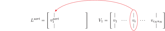
      Figure 1:                     STEP 3.1. Choosing the starting vector.

   2. Compute $\epsilon_{1k}={v_{1}^{sort}}^{\dagger}\rho_{2}v_{k}$ for another column $v_{k}$ of $V_{1}$ and if $\epsilon_{1k}\neq 0$, move $v_{k}$ into the list $L^{sort}$ and rename it as $v_{2}^{sort}$. Repeat on all remaining columns of $V_{1}$, move those $v_{k}$ with ${v_{1}^{sort}}^{\dagger}\rho_{2}v_{k}\not=0$ into the list $L^{sort}$ and label them as $v_{j}^{sort}$, with the index $j$ reflecting the order in which they have been included into the list.

      

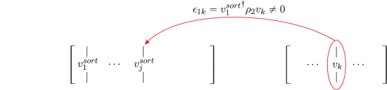
      Figure 2:                      STEP 3.2. Finding vectors in the same subspace as $v_{1}^{sort}$.

   3. Compute $\epsilon_{jk}={v_{j}^{sort}}^{\dagger}\rho_{2}v_{k}$ for $v_{j}^{sort}\in L^{sort},\ j\geq 2$, for those columns $v_{k}$ of $V_{1}$ not yet moved into $L^{sort}$ in STEP 3.2. This is a re-check since there might be some vector left not included in the list in STEP 3.2 because it happened to be orthogonal to $v_{1}^{sort}$ in the scalar product defined by $\rho_{2}$. The mutual genericity condition ensures that no vector in $L^{sort}$ can be orthogonal to all remaining vectors in the list.

      

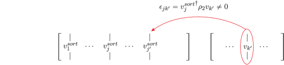
      Figure 3:                         STEP 3.3. Finding the remaining vectors in the same subspace as $v_{1}^{sort}$.

   4. Once we have finished verifying all eigenvectors in $L^{sort}$, we take a block whose columns are the eigenvectors in $L^{sort}$ and denote it as $L^{1}$, since it is a set of $c_{1}n_{1}$ vectors constituting an orthonormal basis of $\mathcal{L}^{1}$. After that, we come back to STEP 3.1 and repeat the process with the rest of vectors until all of them have been sorted.

   At the end of this step, we obtain a matrix we may call $V_{1}^{sort_{1}}$ whose columns form bases $L^{\alpha}$ of the proper subspaces $\mathcal{L}^{\alpha}$ for $\alpha=1,\ldots,N$, i.e.,

   $$\begin{array}[]{cccc}V_{1}^{sort_{1}}=\left(\begin{array}[]{c|c|c|c}L^{1}&\,\,L^{2}&\,\cdots&\,\,L^{N}\end{array}\right).\vspace{-0.5cm}\\ \underbrace{\phantom{a..}}_{c_{1}n_{1}}&\underbrace{\phantom{aa}}_{c_{2}n_{2}}&\hskip 17.07182pt\underbrace{\phantom{aa.}}_{c_{N}n_{N}}\end{array}$$

   This step also gives the dimensions $c_{\alpha}n_{\alpha}$ by counting the number of vectors in each subspace.

4. Second sorting: Reorder the columns within each $L^{\alpha}$ grouping together the eigenvectors corresponding to the same eigenvalue of $\rho_{1}$. To do this, we just reorder the eigenvectors in each $L^{\alpha}$ in decreasing order corresponding to their eigenvalues. Thus, we obtain:

   $$V_{1}^{sort}=\left(\begin{array}[]{c|c|c|c}{L^{1}}^{sort}&{L^{2}}^{sort}&\,\cdots&{L^{N}}^{sort}\end{array}\right),$$

   where

   $${{L^{\alpha}}^{sort}}^{\dagger}\rho_{1}{L^{\alpha}}^{sort}=\mathrm{diag}\left(\lambda_{1}^{\alpha}\mathds{1}_{c_{\alpha}},\lambda_{2}^{\alpha}\mathds{1}_{c_{\alpha}},\ldots,\lambda_{n_{\alpha}}^{\alpha}\mathds{1}_{c_{\alpha}}\right)\,.$$

   Counting the multiplicity of one eigenvalue in each $\alpha$ will give the multiplicity $c_{\alpha}$. Hence, since we already got the products $c_{\alpha}n_{\alpha}$ in STEP 3, we can also get the dimensions of the irreps $n_{\alpha}$ by dividing those numbers by $c_{\alpha}$. At this point, it is also possible, if needed, to obtain the characters of the irreps in the decomposition of $D(h)$ by computing

   $$\chi^{\alpha}(h)=\frac{1}{c_{\alpha}}\mathrm{Tr}\big{(}{{L^{\alpha}}^{sort}}^{\dagger}D(h){L^{\alpha}}^{sort}\big{)}\,.$$

5. Coarse block-diagonalization of $\bm{\rho_{2}}$: Compute the matrix $V_{1}^{sort^{\dagger}}\rho_{2}\,V_{1}^{sort}$ to obtain the coarse block-diagonalization of $\rho_{2}$ in terms of the matrices $\Sigma^{\alpha}$, as shown in Corollary III.2, and identify the square matrices $R_{ij},\ i,j=1,\ldots,n_{\alpha}$, of size $c_{\alpha}$.

6. Compute a matrix $\widetilde{R}$: According to Corollary III.3, for each $\Sigma^{\alpha}$ choose a column of matrices $\widetilde{R}_{jk_{\alpha}}^{\alpha}$ such that $\widetilde{R}_{jk_{\alpha}}^{\alpha}\neq 0$ for all $j=1,\ldots,n_{\alpha}$, compute the unitary matrices

   $$\widetilde{R}_{k_{\alpha}}^{\alpha}=\mathrm{diag}\left(\widetilde{R}_{1k_{\alpha}}^{\alpha},\widetilde{R}_{2k_{\alpha}}^{\alpha},\ldots,\widetilde{R}_{n_{\alpha}k_{\alpha}}^{\alpha}\right)$$

   and finally compute the unitary matrix

   $$\widetilde{R}=\mathrm{diag}\left(\widetilde{R}_{k_{1}}^{1},\widetilde{R}_{k_{2}}^{2},\ldots,\widetilde{R}_{k_{N}}^{N}\right).$$

7. Compute the permutation matrix $F$: Matrices $F^{\alpha}$ will be the matrix $F$ in Lemma III.4 with $c=c_{\alpha}$ and $n=n_{\alpha}$, then compute those matrices for each $\alpha$ and collect them in the block diagonal matrix:

   $$\widetilde{F}=\mathrm{diag}\left(F^{1},F^{2},\ldots,F^{N}\right).$$

8. Final rearrangement: Compute the Clebsch–Gordan matrix $\widehat{C}=V_{1}^{sort}\widetilde{R}\widetilde{F}$.

V Some examples

V.1 Decomposition of the regular representation of a finite group

The algorithm we have presented decomposes any finite-dimensional unitary representation of any compact Lie group. In the case of finite groups, it is natural to apply it to the regular representation because it contains every irreducible representation with multiplicity equal to the dimension of its irreps, $c_{\alpha}=n_{\alpha}$ [Se77, , Ch. 2], thus:

$$|G|=\sum_{\alpha=1}^{N}n_{\alpha}^{2}.$$

The regular representation of a group $G$ is the unitary representation obtained from the action of the group $G$ on the Hilbert space of square integrable functions on the group, $\mathcal{H}=L^{2}(G,\mu)$, where $\mu$ denotes the left(right)-invariant Haar measure by left(right) translations.

As before, we will restrict the discussion to finite groups $G$ as in Sect. II. The space of square integrable functions on $G$ can be identified canonically with the $|G|$-dimensional complex space formally generated by the elements of the group, i.e., we will denote by $\mathbb{C}[G]$ the linear space whose elements are given by $a=\sum_{g\in G}a_{g}g$, $a_{g}\in\mathbb{C}$, $g\in G$, with the natural addition law $a+b=\sum_{g\in G}(a_{g}+b_{g})g$. Notice that $\mathbb{C}[G]$ carries also a natural associative algebra:

$$a\cdot b=\sum_{g,g^{\prime}\in G}a_{g}b_{g^{\prime}}gg^{\prime}=\sum_{g\in G}(\sum_{g^{\prime}\in G}a_{gg^{\prime-1}}b_{g^{\prime}})g\,,$$

although we will not make use of such structure here.

The left regular representation is defined as:

$$U^{reg}(g)a=\sum_{g^{\prime}\in G}a_{g^{\prime}}gg^{\prime}=\sum_{g^{\prime}\in G}a_{g^{-1}g^{\prime}}g^{\prime}\,.$$

Thus, the matrix elements of the regular representation are obtained by computing the action of the group on the orthonormal basis $g_{i}$, $i=0,\ldots,n-1$, of the Hilbert space $\mathcal{H}=\mathbb{C}[G]$:

$$D^{reg}_{ij}(g_{k})=\langle g_{i},U^{reg}(g_{k})g_{j}\rangle=\langle g_{i},g_{k}g_{j}\rangle.$$

Then, the matrix representation of the left regular representation of the element $g_{k}$ can be easily computed from the table of the group written below (notice the inverse of the elements along the rows). The matrix $D^{reg}(g_{k})$ is obtained by constructing a matrix with ones in the positions where $g_{k}$ appears in the table and zeros in the rest.

$\begin{matrix}\\ \vspace{-0.35cm}\end{matrix}$T	$e$	$g_{1}^{-1}$	$\cdots$	$g_{i}^{-1}$	$\cdots$	$g_{n-1}^{-1}$
$\begin{matrix}\\ \vspace{-0.3cm}\end{matrix}$ $e$	$e$	$g_{1}^{-1}$	$\cdots$	$g_{i}^{-1}$	$\cdots$	$g_{n-1}^{-1}$
$g_{1}$	$g_{1}$	$e$	$\cdots$	$g_{1}g_{i}^{-1}$	$\cdots$	$g_{1}g_{n-1}^{-1}$
$\vdots$	$\vdots$	$\vdots$	$\cdot$	⋮		$\vdots$
$g_{i}$	$g_{i}$	$g_{i}g_{1}^{-1}$		​$e$		$g_{i}g_{n-1}^{-1}$
$\vdots$	$\vdots$	$\vdots$		⋮	$\cdot$	$\vdots$
$g_{n-1}$	$g_{n-1}$	$g_{n-1}g_{1}^{-1}$	$\cdots$	$g_{n-1}g_{i}^{-1}$	$\cdots$	$e$  .

Table 1: Group table.

In the case of the regular representation, the input of our program can be the matrix $T$ constructed out of the table T (see TABLE 1) relabeled by identifying $e$ with $1$ and $g_{i}$ with $i+1$ and whose entries are defined as:

$$T_{ij}=k\,,\quad\mathrm{if}\quad g_{i-1}g_{j-1}^{-1}=g_{k-1}\,,\qquad i,j,k=1,\ldots,n\,.$$ (22)

Once we have the group multiplication table in this form, we do not need to compute explicitly the regular representation for each element $D^{reg}(g)$ to create the adapted states $\rho_{1}$ and $\rho_{2}$ in STEP 1, since we can simply evaluate the random vectors $\bm{\varphi}_{a}$ on the elements of the table, that is,

$$[\tau_{a}]_{ij}=\bm{\varphi}_{a}\big{(}T_{ij}\big{)}\,,\qquad a=1,2\,.$$ (23)

In the final Appendix, we will show the results obtained using our algorithm for the decomposition of the regular representation in two simple cases: the permutation group $S_{3}$ and the alternating group $A_{4}$.

To verify the accuracy of the results, we will compare characters, since they are independent of the choice of basis. We shall compute the characters $\widehat{\chi}^{\alpha}$ of the irreps obtained after applying the unitary transformation $\widehat{C}$ provided by our algorithm and we will compare them with the exact characters $\chi^{\alpha}_{exact}$ by defining the error as:

$$\widehat{\chi}_{error}=\frac{1}{|H|}\max_{\alpha\in\widehat{H}}\sum_{h\in H}|\chi^{\alpha}_{exact}(h)-\widehat{\chi}^{\alpha}(h)|\,,$$ (24)

where $\widehat{H}$ is the family of equivalence classes of irreps of $H$.

V.2 Clebsch–Gordan coefficients of $SU(2)$

Let $G$ be a compact Lie group and $H$ a closed subgroup (hence, compact too). States adapted to $H$ will have the form:

$$\rho=\frac{1}{Z}\int_{H}\overline{\chi_{\rho}(h)}D(h)\textrm{d}h\,,$$ (25)

where $Z$ is the normalization factor

$$Z=\int_{H}\overline{\chi_{\rho}(h)}\chi(h)\textrm{d}h\,,$$

and $\textrm{d}h$ denotes the invariant Haar measure on $H$.

Because our algorithm is numerical, we need to approximate the integral (25) with a finite sum. Choosing a quadrature rule to approximate the integral (25) for a given $\rho$ is equivalent to use another $\widehat{\rho}$ such that $\chi_{\widehat{\rho}}\neq 0$ only at a finite number of elements of the group. Then, the integral (25) for $\widehat{\rho}$ reduces to a finite sum and the approximation of $\widehat{\rho}$ is exact. It could happen that the generic adapted states thus obtained do not have enough degrees of freedom, i.e., it might happen that the block diagonal matrices of the representation were not irreducible. However, we will see that this is not a problem because in the case of Lie groups, the Clebsch–Gordan matrix decomposing all the elements of its Lie algebra $\mathfrak{g}$ will be the Clebsch–Gordan matrix decomposing all the elements of the representation.

For compact Lie groups, the elements of a unitary representation are related via the exponential map with the corresponding representation via Hermitean matrices of elements of its Lie algebra $\mathfrak{g}$: $U(g)=\mathrm{e}^{is\xi}$, $s\in\mathds{R}$ and $\xi\in\mathfrak{g}$.

One can immediately see that the Clebsch–Gordan matrix $C$ that decomposes the matrices representing all the elements of the Lie algebra $\xi\in\mathfrak{g}$ will decompose all the elements of the unitary representation and vice versa:

$$C^{\dagger}\xi_{i}C=\mathds{1}_{c_{1}}\otimes\xi_{i}^{1}\oplus\cdots\oplus\mathds{1}_{c_{N}}\otimes\xi_{i}^{N}\Longleftrightarrow\;C^{\dagger}U(g)C=\mathds{1}_{c_{1}}\otimes U^{1}(g)\oplus\cdots\oplus\mathds{1}_{c_{N}}\otimes U^{N}(g)\,,$$

where $\{\xi_{i}^{\alpha}\}_{i=1}^{n_{\mathfrak{g}}}$, $\alpha=1,\ldots,N$, are the matrices representing a set of generators of the Lie algebra $\mathfrak{g}$ ($n_{\mathfrak{g}}$ is the dimension of the set) and $U^{\alpha}(g),\ \alpha=1,\ldots,N$, their corresponding unitary representations.

The original Clebsch–Gordan problem consists in reducing a tensor product representation $U_{A}(g)\otimes U_{B}(g)$, $\forall g\in G$, of two representations of the same group $G$ restricted to the diagonal subgroup of the product group. By associativity, this problem can be generalized to any number of tensor product factors $U^{1}(g)\otimes U^{2}(g)\otimes\cdots\otimes U^{n}(g)$. The associated Lie algebra generators will be given by:

$$\xi_{i}=\xi_{i}^{1}\otimes\mathds{1}^{2}\otimes\cdots\otimes\mathds{1}^{n}+\mathds{1}^{1}\otimes\xi_{i}^{2}\otimes\cdots\otimes\mathds{1}^{n}+\cdots+\mathds{1}^{1}\otimes\mathds{1}^{2}\otimes\cdots\otimes\xi_{i}^{n},$$

with commutation relations given by:

$$[\xi_{i},\xi_{j}]=c_{ij}^{k}\xi_{k},\qquad[\xi_{i}^{\alpha},\xi_{i}^{\alpha}]=c_{ij}^{k}\xi_{i}^{\alpha},\qquad\alpha=1,\ldots,n,\qquad i,j,k=1,\ldots,n_{\mathfrak{g}},\qquad c_{ij}^{k}\in\mathds{C}.$$

Let us now study the $SU(2)$ group: the generators of the representation of its associated Lie algebra $\mathfrak{su}(2)$ are given by the Hermitian traceless angular momentum operators $J_{k}$ satisfying the commutation relations

$$[J_{i},J_{j}]=i\epsilon_{ij}^{k}J_{k}\,,\qquad i,j,k=x,y,z\,,\qquad n_{\mathfrak{g}}=3\,.$$ (26)

Its associated representation of $SU(2)$ can be written as:

$$D(\bm{s})=\textrm{e}^{i\bm{s}\cdot\bm{J}}\,,\qquad\bm{s}=(s_{x},s_{y},s_{z})\in\mathds{R}^{3}.$$ (27)

The matrix representation of momentum $j$ of the angular momentum operators $J_{i}$ is usually written in a basis of eigenvectors of $J_{z}$,

$$J_{z}|j,m\rangle=m|j,m\rangle\,,\qquad m=j,j-1,\ldots,-j\,,$$

and the representation of the operators $J_{x}$ and $J_{y}$ is usually obtained from the representation of the ladder operators $J_{\pm}=J_{x}\pm iJ_{y}$,

$$\langle j,m|J_{\pm}|j,m^{\prime}\rangle=\sqrt{(j\mp m^{\prime})(j\pm m^{\prime}+1)}\,\delta_{mm^{\prime}\pm 1}\,.$$ (28)

For instance, if $j=3/2$:

$$J_{x}=\begin{pmatrix}0&\frac{\sqrt{3}}{2}&0&0\\ \frac{\sqrt{3}}{2}&0&1&0\\ 0&1&0&\frac{\sqrt{3}}{2}\\ 0&0&\frac{\sqrt{3}}{2}&0\end{pmatrix}\,,\qquad J_{y}=\begin{pmatrix}0&-i\frac{\sqrt{3}}{2}&0&0\\ i\frac{\sqrt{3}}{2}&0&-i&0\\ 0&i&0&-i\frac{\sqrt{3}}{2}\\ 0&0&i\frac{\sqrt{3}}{2}&0\end{pmatrix},$$

$$J_{z}=\begin{pmatrix}\frac{3}{2}&0&0&0\\ 0&\frac{1}{2}&0&0\\ 0&0&-\frac{1}{2}&0\\ 0&0&0&-\frac{3}{2}\end{pmatrix}\,,$$

in the standard basis

$$|3/2,3/2\rangle=\begin{pmatrix}1\\ 0\\ 0\\ 0\end{pmatrix}\,,\quad|3/2,1/2\rangle=\begin{pmatrix}0\\ 1\\ 0\\ 0\end{pmatrix}\,,\quad|3/2,-1/2\rangle=\begin{pmatrix}0\\ 0\\ 1\\ 0\end{pmatrix}\,,\quad|3/2,-3/2\rangle=\begin{pmatrix}0\\ 0\\ 0\\ 1\end{pmatrix}\,.$$

The standard Clebsch–Gordan matrix is constructed with eigenvectors of the total angular momentum operator $J_{T}$ with respect to the $z$ component,

$${J_{T}}_{z}=J^{1}_{z}\otimes\mathds{1}^{2}\otimes\cdots\otimes\mathds{1}^{n}+\mathds{1}^{1}\otimes J^{2}_{z}\otimes\cdots\otimes\mathds{1}^{n}+\cdots+\mathds{1}^{1}\otimes\mathds{1}^{2}\otimes\cdots\otimes J^{n}_{z}\,,$$

where $n$ is the number of parts of the system. The eigenvectors of this operator are usually denoted by $|J,M\rangle$, where $J$ represent the total angular momentum and $M=J,J-1,\ldots,-J$ the corresponding eigenvalues:

$${J_{T}}_{z}|J,M\rangle=M|J,M\rangle\,.$$

The standard procedure to obtain this Clebsch–Gordan matrix consists in applying successively the ladder operator $J_{-}$ starting from the state of maximum momentum $|J_{max},M_{max}\rangle=|j_{1}+j_{2},j_{1}+j_{2}\rangle$. Notice that since the action of the matrix elements of the ladder operators (28) is real, the Clebsh-Gordan coefficients are real too.

Recall that the Clebsch–Gordan matrix provided by our algorithm is written in terms of the eigenvectors of the first adapted state $\rho_{1}$. Thus, if we want to compare the Clebsch–Gordan coefficients obtained from our algorithm with the standard ones, we have to find a Clebsch–Gordan matrix $C_{z}$ which is conformed by eigenvectors of the operator ${J_{T}}_{z}$. To do that, we first create two real adapted states using the fact that the operators $J_{k}$ verify:

$${J}^{*}_{x}=J_{x}\,,\quad{J}^{*}_{y}=-J_{y}\,,\quad{J}^{*}_{z}=J_{z}\,,$$

where ^∗ denotes the complex conjugate. Therefore, for any adapted state $\rho$, its complex conjugate $\rho^{*}$ is an adapted state too. Hence, to create real adapted states, we first add to each matrix $\tau_{a}$, $a=1,2$, in STEP 1 in Section IV, its complex conjugate to obtain real symmetric matrices, and then we multiply the result by its transpose to make it positive definite. Finally, we normalize them, dividing by their trace, i.e.,

$$\tilde{\rho}_{a}=\tau_{a}+\tau^{*}_{a}\,,\qquad{\rho_{real}}_{a}=\frac{1}{\mathrm{Tr}(\tilde{\rho}_{a}\tilde{\rho}_{a}^{t})}\tilde{\rho}_{a}\tilde{\rho}_{a}^{t}.$$ (29)

Once we have two real adapted states ${\rho_{real}}_{1}$ and ${\rho_{real}}_{2}$, we apply our algorithm to get the real Clebsch–Gordan matrix $\widehat{C}$. After that, we transform the operator ${J_{T}}_{z}$ with $\widehat{C}$ to decompose it into irreducible representations,

$$\widehat{C}^{\dagger}{J_{T}}_{z}\widehat{C}=\left(\begin{array}[]{ccccc}\begin{array}[]{|cc|}\hline\cr\phantom{a}*&\hskip 8.5359pt*\phantom{a}\\ \phantom{a}*&\hskip 8.5359pt*\phantom{a}\\ \hline\cr\end{array}&&&&\\ &\begin{array}[]{|cccc|}\hline\cr\phantom{a}*&\hskip 8.5359pt*&\hskip 8.5359pt*&\hskip 8.5359pt*\phantom{a}\\ \phantom{a}*&\hskip 8.5359pt*&\hskip 8.5359pt*&\hskip 8.5359pt*\phantom{a}\\ \phantom{a}*&\hskip 8.5359pt*&\hskip 8.5359pt*&\hskip 8.5359pt*\phantom{a}\\ \phantom{a}*&\hskip 8.5359pt*&\hskip 8.5359pt*&\hskip 8.5359pt*\phantom{a}\\ \hline\cr\end{array}&&&\\ &&\ddots&&\\ &&&\hskip 5.69046pt\ddots&\\ &&&&\hskip 1.42271pt\begin{array}[]{|ccc|}\hline\cr\phantom{a}*&\hskip 8.5359pt*&\hskip 8.5359pt*\phantom{a}\\ \phantom{a}*&\hskip 8.5359pt*&\hskip 8.5359pt*\phantom{a}\\ \phantom{a}*&\hskip 8.5359pt*&\hskip 8.5359pt*\phantom{a}\\ \hline\cr\end{array}\end{array}\right)\,,$$ (30)

and we diagonalize each block of this matrix transforming it with a block-diagonal matrix $V_{z}$ which reorders the eigenvalues as follows:

$$V_{z}^{\dagger}\widehat{C}^{\dagger}{J_{T}}_{z}\widehat{C}V_{z}=\begin{pmatrix}j_{1}&&&&&&&&&\\ &j_{1}-1&&&&&&&&\\ &&\rotatebox{-48.0}{\makebox[0.0pt]{\makebox[10.00002pt]{\xleaders\hbox{$\cdot$\hskip 0.89996pt}\hfill\kern 0.0pt}}}&&&&&&&\\ &&&-j_{1}&&&&&&\\ &&&&j_{2}&&&&&\\ &&&&&j_{2}-1&&&&\\ &&&&&&\rotatebox{-48.0}{\makebox[0.0pt]{\makebox[10.00002pt]{\xleaders\hbox{$\cdot$\hskip 0.89996pt}\hfill\kern 0.0pt}}}&&&\\ &&&&&&&-j_{2}&&\\ &&&&&&&&\hskip 4.55254pt\rotatebox{-48.0}{\makebox[0.0pt]{\makebox[10.00002pt]{\xleaders\hbox{$\cdot$\hskip 0.89996pt}\hfill\kern 0.0pt}}}&\\ &&&&&&&&&\rotatebox{-48.0}{\makebox[0.0pt]{\makebox[10.00002pt]{\xleaders\hbox{$\cdot$\hskip 0.89996pt}\hfill\kern 0.0pt}}}\\ &&&&&&&&&j_{N}\\ &&&&&&&&&\hskip 19.91684ptj_{N}-1\\ &&&&&&&&&\hskip 45.52458pt\rotatebox{-48.0}{\makebox[0.0pt]{\makebox[10.00002pt]{\xleaders\hbox{$\cdot$\hskip 0.89996pt}\hfill\kern 0.0pt}}}\\ &&&&&&&&&\hskip 71.13188pt-j_{N}\\ \end{pmatrix}\,.$$ (31)

Therefore, the Clebsch–Gordan matrix whose columns are the eigenvectors of ${J_{T}}_{z}$, reordered in this way, is given by

$$C_{z}=\widehat{C}V_{z}\,.$$ (32)

In the Appendix, we will show the computation of the Clebsch–Gordan coefficients for the bipartite spin system $3/2\times 1$ and for the tripartite spin system $1/2\times 1/2\times 3/2$. Again, we will verify the accuracy by comparing the exact characters with the ones computed after transforming with the Clebsch–Gordan matrix obtained with our algorithm. For any irreducible representation of the $SU(2)$ group, it can be shown that the characters have the following expression:

$$\chi^{n}_{exact}(\bm{s})=\begin{cases}\displaystyle{2\sum\limits_{k=1}^{n/2}\cos\left(\sqrt{s_{x}^{2}+s_{y}^{2}+s_{z}^{2}}\left(\frac{n-1}{2}-k+1\right)\right)}\,,&\text{$n$ even,}\\ \displaystyle{2\sum\limits_{k=1}^{(n-1)/2}\cos\left(\sqrt{s_{x}^{2}+s_{y}^{2}+s_{z}^{2}}\left(\frac{n-1}{2}-k+1\right)\right)+1}\,,&\text{$n$ odd},\end{cases}$$ (33)

where $n=2j+1$ is the dimension of the irrep. Therefore, we measure the accuracy through

$$\widehat{\chi}_{error}=\max_{\alpha\in\widehat{H}}\int_{H}|\chi^{\alpha}_{exact}(h)-\widehat{\chi}^{\alpha}(h)|\textrm{d}h\approx\frac{1}{N_{H}}\sum_{i=1}^{N_{H}}|\chi^{\alpha}_{exact}(h)-\widehat{\chi}^{\alpha}(h)|\,,$$ (34)

with $N_{H}$ the number of elements in the quadrature approximation.

VI Conclusions and discussion

A numerical algorithm to compute the decomposition of a finite-dimensional unitary representation of a compact Lie group has been presented. Such algorithm uses the notion of generic adapted quantum mixed states to obtain the block structure and, eventually, the coefficients of the Clebsch–Gordan matrix solving the decomposition problem.

The numerical algorithm is stable and accurate, since it combines nothing but stable routines involving diagonalization of Hermitian matrices, sorting and recombination of matrix blocks and matrix products. The numerical examples presented confirm this.

The algorithm has been used successfully to decompose the regular representation of two finite groups and the direct product of two and three representations of $SU(2)$. In the first case, the main computational task was to prepare the group table, a preliminary task before the algorithm is used. In the second case, this preliminary part was much easier, since explicit expressions of the representations of the Lie algebra $\mathfrak{su}(2)$, for any value of spin, are well-known.

The algorithm can be easily extended to finite-dimensional representations of non-compact groups. However, because the representations will cease to be unitary, the numerical stability of the algorithm could be compromised. Further insights on these questions will be considered elsewhere.

Appendix

In this appendix, we present the results obtained for the decomposition of the $S_{3}$ and $A_{4}$ group, and the Clebsch–Gordan coefficients of the spin systems $3/2\times 1$ and $1/2\times 1/2\times 3/2$. All experiments were conducted using Matlab R2012a (version 7.14.0.739).

A.1.  The decomposition of the left regular representation of the permutation group $S_{3}$.

The $S_{3}$ group is the group of permutations of three elements and it has order six. The elements of this group can be generated with the set of transpositions $a_{k}=(k,k+1)$, $k=1,2$:

$$a_{1}^{2}=a_{2}^{2}=(a_{1}a_{2})^{3}=e\,.$$

Our algorithm decomposes the regular representation into two representations $\widehat{D}^{1}$ and $\widehat{D}^{2}$ of dimension one and multiplicity one, and another one $\widehat{D}^{3}$ of dimension two and multiplicity two, exactly as expected. The representation $\widehat{D}^{1}$ corresponds to the trivial one, $\widehat{D}^{1}(g)=1$, $\forall g\in S_{3}$, and the rest of representations obtained after applying the transformation $\widehat{C}$ are the following:

$$\begin{array}[]{c!{\vrule width 1.5pt}c!{\vrule width 1pt}c|}S_{3}\hfil\lx@intercol\vrule width=&\widehat{D}^{2}\hfil\lx@intercol\vrule width=1.0&\widehat{D}^{3}\\ \hrule height=1.5pt\cr\begin{matrix}\phantom{a}\\ e\\ \phantom{a}\end{matrix}\hfil\lx@intercol\vrule width=&\begin{matrix}\phantom{a}\\ 1.0000\\ \phantom{a}\end{matrix}\hfil\lx@intercol\vrule width=1.0&\begin{pmatrix}1.0000&0.0000+0.0000i\\ 0.0000-0.0000i&1.0000\end{pmatrix}\\ \hrule\cr\begin{matrix}\phantom{a}\\ a_{1}\\ \phantom{a}\end{matrix}\hfil\lx@intercol\vrule width=&\begin{matrix}\phantom{a}\\ -1.0000\\ \phantom{a}\end{matrix}\hfil\lx@intercol\vrule width=1.0&\begin{pmatrix}-0.7501&0.6399-0.1671i\\ 0.6399+0.1671i&0.7501\end{pmatrix}\\ \hrule\cr\end{array}$$

$$\begin{array}[]{c!{\vrule width 1.5pt}c!{\vrule width 1pt}c|}S_{3}\hfil\lx@intercol\vrule width=&\widehat{D}^{2}\hfil\lx@intercol\vrule width=1.0&\widehat{D}^{3}\\ \hrule height=1.5pt\cr\begin{matrix}\phantom{a}\\ a_{2}\\ \phantom{a}\end{matrix}\hfil\lx@intercol\vrule width=&\begin{matrix}\phantom{a}\\ -1.0000\\ \phantom{a}\end{matrix}\hfil\lx@intercol\vrule width=1.0&\begin{pmatrix}0.3542&-0.5615-0.7479i\\ -0.5615+0.7479i&-0.3542\end{pmatrix}\\ \hrule\cr\begin{matrix}\phantom{a}\\ a_{1}a_{2}\\ \phantom{a}\end{matrix}\hfil\lx@intercol\vrule width=&\begin{matrix}\phantom{a}\\ 1.0000\\ \phantom{a}\end{matrix}\hfil\lx@intercol\vrule width=1.0&\begin{pmatrix}-0.5000+0.5723i&0.1945+0.6202i\\ -0.1945+0.6202i&-0.5000-0.5723i\end{pmatrix}\\ \hrule\cr\begin{matrix}\phantom{a}\\ a_{2}a_{1}\\ \phantom{a}\end{matrix}\hfil\lx@intercol\vrule width=&\begin{matrix}\phantom{a}\\ 1.0000\\ \phantom{a}\end{matrix}\hfil\lx@intercol\vrule width=1.0&\begin{pmatrix}-0.5000-0.5723i&-0.1945-0.6202i\\ 0.1945-0.6202i&-0.5000+0.5723i\end{pmatrix}\\ \hrule\cr\begin{matrix}\phantom{a}\\ a_{2}a_{1}a_{2}\\ \phantom{a}\end{matrix}\hfil\lx@intercol\vrule width=&\begin{matrix}\phantom{a}\\ -1.0000\\ \phantom{a}\end{matrix}\hfil\lx@intercol\vrule width=1.0&\begin{pmatrix}0.3959&-0.0784+0.9149i\\ -0.0784-0.9149i&-0.3959\end{pmatrix}\\ \hrule\cr\end{array}$$

Table 2: Irreducible representations obtained for $S_{3}$ group.

If we use the formula (24) to compute the accuracy of the characters of the irreps, we obtain:

$$\widehat{\chi}_{error}=3.5785\cdot 10^{-15}\,.$$

A.2.  The decomposition of the left regular representation of the alternating group $A_{4}$.

The alternating group $A_{4}$ is the group of even permutations of four elements. This group has twelve elements and it can be generated with three generators satisfying the relations

$$a^{2}=b^{2}=c^{3}=(ab)^{2}=ac^{2}abc=bc^{2}ac=e.$$

The left regular representation of this group has four irreducible representations: three of dimension one and one of dimension three. Hence, our algorithm will decompose the regular representation of this group into the three representations of dimension one with multiplicity one and the representation of dimension three with multiplicity three. Again, $\widehat{D}^{1}$ is the trivial representation $\widehat{D}^{1}(g)=1$, $\forall g\in A_{4}$, and the rest are given by:

$$\begin{array}[]{c!{\vrule width 1.5pt}c!{\vrule width 1pt}c!{\vrule width 1pt}c|}A_{4}\hfil\lx@intercol\vrule width=&\widehat{D}^{2}\hfil\lx@intercol\vrule width=1.0&\widehat{D}^{3}\hfil\lx@intercol\vrule width=1.0&\widehat{D}^{4}\\ \hrule height=1.5pt\cr\begin{matrix}\vspace{0.2cm}\phantom{a}\\ e\\ \vspace{0.2cm}\phantom{a}\end{matrix}\hfil\lx@intercol\vrule width=&\begin{matrix}\vspace{0.2cm}\phantom{a}\\ 1.0000\\ \vspace{0.2cm}\phantom{a}\end{matrix}\hfil\lx@intercol\vrule width=1.0&\begin{matrix}\vspace{0.2cm}\phantom{a}\\ 1.0000\\ \vspace{0.2cm}\phantom{a}\end{matrix}\hfil\lx@intercol\vrule width=1.0&\begin{pmatrix}1.0000&-0.0000+0.0000i&-0.0000-0.0000i\\ -0.0000-0.0000i&1.0000&0.0000+0.0000i\\ -0.0000+0.0000i&0.0000-0.0000i&1.0000\end{pmatrix}\\ \hrule\cr\begin{matrix}\vspace{0.2cm}\phantom{a}\\ a\\ \vspace{0.2cm}\phantom{a}\end{matrix}\hfil\lx@intercol\vrule width=&\begin{matrix}\vspace{0.2cm}\phantom{a}\\ 1.0000\\ \vspace{0.2cm}\phantom{a}\end{matrix}\hfil\lx@intercol\vrule width=1.0&\begin{matrix}\vspace{0.2cm}\phantom{a}\\ 1.0000\\ \vspace{0.2cm}\phantom{a}\end{matrix}\hfil\lx@intercol\vrule width=1.0&\begin{pmatrix}-0.9852&-0.0240+0.0941i&0.1176+0.0789i\\ -0.0240-0.0941i&-0.3653&0.3099-0.8724i\\ 0.1176-0.0789i&0.3099+0.8724i&0.3504\end{pmatrix}\\ \hrule\cr\begin{matrix}\vspace{0.2cm}\phantom{a}\\ b\\ \vspace{0.2cm}\phantom{a}\end{matrix}\hfil\lx@intercol\vrule width=&\begin{matrix}\vspace{0.2cm}\phantom{a}\\ 1.0000\\ \vspace{0.2cm}\phantom{a}\end{matrix}\hfil\lx@intercol\vrule width=1.0&\begin{matrix}\vspace{0.2cm}\phantom{a}\\ 1.0000\\ \vspace{0.2cm}\phantom{a}\end{matrix}\hfil\lx@intercol\vrule width=1.0&\begin{pmatrix}0.6482&-0.2501+0.4766i&-0.3940-0.3672i\\ -0.2501-0.4766i&-0.8242&-0.0464+0.1697i\\ -0.3940+0.3672i&-0.0464-0.1697i&-0.8240-0.0000i\end{pmatrix}\\ \hrule\cr\begin{matrix}\vspace{0.2cm}\phantom{a}\\ c\\ \vspace{0.2cm}\phantom{a}\end{matrix}\hfil\lx@intercol\vrule width=&\begin{matrix}\vspace{-0.2cm}\phantom{a}\\ \!\!-0.5000\\ \,+0.866i\\ \vspace{-0.2cm}\phantom{a}\end{matrix}\hfil\lx@intercol\vrule width=1.0&\begin{matrix}\vspace{-0.2cm}\phantom{a}\\ \!\!-0.5000\\ \,\,-0.8660i\\ \vspace{-0.2cm}\phantom{a}\end{matrix}\hfil\lx@intercol\vrule width=1.0&\begin{pmatrix}-0.1137-0.4209i&-0.4113-0.2302i&0.4649-0.6096i\\ -0.0136+0.5419i&0.0028+0.5742i&0.5988-0.1335i\\ -0.6284+0.3482i&0.4483-0.4971i&0.1110-0.1533i\end{pmatrix}\\ \hrule\cr\begin{matrix}\vspace{0.2cm}\phantom{a}\\ c^{2}\\ \vspace{0.2cm}\phantom{a}\end{matrix}\hfil\lx@intercol\vrule width=&\begin{matrix}\vspace{-0.2cm}\phantom{a}\\ \!\!-0.5000\\ \,\,-0.8660i\\ \vspace{-0.2cm}\phantom{a}\end{matrix}\hfil\lx@intercol\vrule width=1.0&\begin{matrix}\vspace{-0.2cm}\phantom{a}\\ \!\!-0.5000\\ \,+0.8660i\\ \vspace{-0.2cm}\phantom{a}\end{matrix}\hfil\lx@intercol\vrule width=1.0&\begin{pmatrix}-0.1137+0.4209i&-0.0136-0.5419i&-0.6284-0.3482i\\ -0.4113+0.2302i&0.0028-0.5742i&0.4483+0.4971i\\ 0.4649+0.6096i&0.5988+0.1335i&0.1110+0.1533i\end{pmatrix}\\ \hrule\cr\begin{matrix}\vspace{0.2cm}\phantom{a}\\ ab\\ \vspace{0.2cm}\phantom{a}\end{matrix}\hfil\lx@intercol\vrule width=&\begin{matrix}\vspace{0.2cm}\phantom{a}\\ 1.0000\\ \vspace{0.2cm}\phantom{a}\end{matrix}\hfil\lx@intercol\vrule width=1.0&\begin{matrix}\vspace{0.2cm}\phantom{a}\\ 1.0000\\ \vspace{0.2cm}\phantom{a}\end{matrix}\hfil\lx@intercol\vrule width=1.0&\begin{pmatrix}-0.6631&0.2741-0.5707i&0.2765+0.2883i\\ 0.2741+0.5707i&0.1895&-0.2635+0.7028i\\ 0.2765-0.2883i&-0.2635-0.7028i&-0.5264\end{pmatrix}\\ \hrule\cr\begin{matrix}\vspace{0.2cm}\phantom{a}\\ cb\\ \vspace{0.2cm}\phantom{a}\end{matrix}\hfil\lx@intercol\vrule width=&\begin{matrix}\vspace{-0.2cm}\phantom{a}\\ \!-0.5000\\ \,+0.8660i\\ \vspace{-0.2cm}\phantom{a}\end{matrix}\hfil\lx@intercol\vrule width=1.0&\begin{matrix}\vspace{-0.2cm}\phantom{a}\\ \!\!-0.5000\\ \,\,-0.8660i\\ \vspace{-0.2cm}\phantom{a}\end{matrix}\hfil\lx@intercol\vrule width=1.0&\begin{pmatrix}-0.0400+0.3917i&0.4431+0.1902i&-0.4347+0.6508i\\ 0.0772+0.4789i&-0.3076-0.7107i&-0.3866-0.1247i\\ -0.7438+0.2375i&-0.4095+0.0115i&0.3475+0.3190i\end{pmatrix}\\ \hrule\cr\end{array}$$

$$\begin{array}[]{c!{\vrule width 1.5pt}c!{\vrule width 1pt}c!{\vrule width 1pt}c|}\hrule\cr\begin{matrix}\vspace{0.2cm}\phantom{a}\\ ca\\ \vspace{0.2cm}\phantom{a}\end{matrix}\hfil\lx@intercol\vrule width=&\begin{matrix}\vspace{-0.2cm}\phantom{a}\\ \!-0.5000\\ \,+0.8660i\\ \vspace{-0.2cm}\phantom{a}\end{matrix}\hfil\lx@intercol\vrule width=1.0&\begin{matrix}\vspace{-0.2cm}\phantom{a}\\ \!\!-0.5000\\ \,\,-0.8660i\\ \vspace{-0.2cm}\phantom{a}\end{matrix}\hfil\lx@intercol\vrule width=1.0&\begin{pmatrix}0.1069+0.3505i&0.8684+0.3002i&-0.1455+0.0155i\\ 0.1273-0.6109i&0.2504+0.2570i&0.6673+0.1914i\\ 0.5625-0.4001i&-0.0133+0.1634i&-0.3573-0.6075i\end{pmatrix}\\ \hrule\cr\begin{matrix}\vspace{0.2cm}\phantom{a}\\ bc\\ \vspace{0.2cm}\phantom{a}\end{matrix}\hfil\lx@intercol\vrule width=&\begin{matrix}\vspace{-0.2cm}\phantom{a}\\ \!\!-0.5000\\ \,+0.866i\\ \vspace{-0.2cm}\phantom{a}\end{matrix}\hfil\lx@intercol\vrule width=1.0&\begin{matrix}\vspace{-0.2cm}\phantom{a}\\ \!\!-0.5000\\ \,\,-0.8660i\\ \vspace{-0.2cm}\phantom{a}\end{matrix}\hfil\lx@intercol\vrule width=1.0&\begin{pmatrix}0.0468-0.3213i&-0.9002-0.2602i&0.1153-0.0567i\\ -0.1908-0.4100i&0.0544-0.1205i&-0.8795+0.0669i\\ 0.8097-0.1857i&-0.0255+0.3222i&-0.1013+0.4419i\end{pmatrix}\\ \hrule\cr\begin{matrix}\vspace{0.2cm}\phantom{a}\\ bc^{2}\\ \vspace{0.2cm}\phantom{a}\end{matrix}\hfil\lx@intercol\vrule width=&\begin{matrix}\vspace{-0.2cm}\phantom{a}\\ \!\!-0.5000\\ \,\,-0.8660i\\ \vspace{-0.2cm}\phantom{a}\end{matrix}\hfil\lx@intercol\vrule width=1.0&\begin{matrix}\vspace{-0.2cm}\phantom{a}\\ \!\!-0.5000\\ \,+0.8660i\\ \vspace{-0.2cm}\phantom{a}\end{matrix}\hfil\lx@intercol\vrule width=1.0&\begin{pmatrix}-0.0400-0.3917i&0.0772-0.4789i&-0.7438-0.2375i\\ 0.4431-0.1902i&-0.3076+0.7107i&-0.4095-0.0115i\\ -0.4347-0.6508i&-0.3866+0.1247i&0.3475-0.3190i\end{pmatrix}\\ \hrule\cr\begin{matrix}\vspace{0.2cm}\phantom{a}\\ cbc\\ \vspace{0.2cm}\phantom{a}\end{matrix}\hfil\lx@intercol\vrule width=&\begin{matrix}\vspace{-0.2cm}\phantom{a}\\ \!\!-0.5000\\ \,\,-0.8660i\\ \vspace{-0.2cm}\phantom{a}\end{matrix}\hfil\lx@intercol\vrule width=1.0&\begin{matrix}\vspace{-0.2cm}\phantom{a}\\ \!\!-0.5000\\ \,+0.8660i\\ \vspace{-0.2cm}\phantom{a}\end{matrix}\hfil\lx@intercol\vrule width=1.0&\begin{pmatrix}0.1069-0.3505i&0.1273+0.6109i&0.5625+0.4001i\\ 0.8684-0.3002i&0.2504-0.2570i&-0.0133-0.1634i\\ -0.1455-0.0155i&0.6673-0.1914i&-0.3573+0.6075i\end{pmatrix}\\ \hrule\cr\begin{matrix}\vspace{0.2cm}\phantom{a}\\ c^{2}b\\ \vspace{0.2cm}\phantom{a}\end{matrix}\hfil\lx@intercol\vrule width=&\begin{matrix}\vspace{-0.2cm}\phantom{a}\\ \!\!-0.5000\\ \,\,-0.8660i\\ \vspace{-0.2cm}\phantom{a}\end{matrix}\hfil\lx@intercol\vrule width=1.0&\begin{matrix}\vspace{-0.2cm}\phantom{a}\\ \!\!-0.5000\\ \,+0.8660i\\ \vspace{-0.2cm}\phantom{a}\end{matrix}\hfil\lx@intercol\vrule width=1.0&\begin{pmatrix}0.0468+0.3213i&-0.1908+0.4100i&0.8097+0.1857i\\ -0.9002+0.2602i&0.0544+0.1205i&-0.0255-0.3222i\\ 0.1153+0.0567i&-0.8795-0.0669i&-0.1013-0.4419i\end{pmatrix}\\ \hrule\cr\end{array}$$

Table 3: Irreducible representations obtained for $A_{4}$ group.

In this case, the accuracy of the characters of the irreps computed with (24) is given by

$$\widehat{\chi}_{error}=4.4888\cdot 10^{-15}.$$

B.1.  Clebsch–Gordan coefficients for the spin system $3/2\times 1$.

Suppose we have a system of two particles in which the first particle has momentum $3/2$ and the second, momentum $1$. It is well known [Ga90, , Ch. 5] that this system is decomposed in the direct sum of systems of momentum $5/2$, $3/2$ and $1/2$, each one with multiplicity one:

$$3/2\times 1=5/2\oplus 3/2\oplus 1/2,$$

or, in other words, that the representation of $SU(2)$ corresponding to the tensor product $3/2\times 1$ has irreducible representations with momentum $5/2$, $3/2$ and $1/2$ with multiplicity one each other.

To create the adapted states for STEP 1 of the algorithm, we have chosen three random vectors $\bm{s}_{i}=({s_{x}}_{i},{s_{y}}_{i},{s_{z}}_{i})$, $\bm{s}_{i}\neq\textbf{0}$, $i=1,2,3$, for each adapted state, to obtain the three linearly independent elements of the representation. Obviously, we have also created two random vectors $\bm{\varphi}_{a}$ of length $3$ to construct the matrices $\tau_{a}$, $a=1,2$ in STEP 1:

$$\tau_{a}=\mathds{1}+\sum_{i=1}^{3}{\varphi_{a}}_{i}D^{3/2}({\bm{s}_{a}}_{i})\otimes D^{1}({\bm{s}_{a}}_{i})\,,$$

where $D^{j_{\alpha}}(\bm{s})$ is the exponential representation given by (27) and $j_{\alpha}$ denotes the momentum of the representation $\alpha$.

To represent the computed Clebsch–Gordan coefficients, we will use the following standard arrangement:

The coefficients obtained for the system $3/2\times 1$ applying the algorithm are shown in the following table:

Table 4: CG coefficients for $3/2\times 1$.

To assess the accuracy, we have approximated the integral in (34) with $N_{H}=50^{3}$. The result we obtained is:

$$\widehat{\chi}_{error}=2.2340\cdot 10^{-16}\,.$$

B.2.  Clebsch–Gordan coefficients for the spin system $1/2\times 1/2\times 3/2$.

To test the capabilities of our algorithm, we will compute the Clebsch–Gordan coefficients of a system of three spin particles. These coefficients can be obtained from suitable choices of coefficients of products of two spins, for that reason, there are no exhaustive tables for systems with more than two particles.

The standard procedure consists in first reducing the representation of the first two particles, then reducing the result with the next particle, and so on, until there are no particles left. In our case, the product of three particles with spin $1/2$, $1/2$ and $3/2$ yields:

$$1/2\otimes 1/2\otimes 3/2=(0\oplus 1)\otimes 3/2=3/2\oplus 5/2\oplus 3/2\oplus 1/2,$$

this is, two irreps of momentum $1/2$ and $5/2$ with multiplicity one and other of momentum $3/2$ with multiplicity two.

In the first step, we block-diagonalize the first two spins:

$$(C_{1/2\otimes 1/2}\otimes\mathds{1}_{4})^{\dagger}(D^{1/2}\otimes D^{1/2}\otimes D^{3/2})(C_{1/2\otimes 1/2}\otimes\mathds{1}_{4})=\big{(}D^{0}\oplus D^{1}\big{)}\otimes D^{3/2}$$

and then, we diagonalize the result:

$$\begin{pmatrix}\mathds{1}_{4}&0\\ 0&C_{1\otimes 3/2}^{\dagger}\end{pmatrix}\left((D^{0}\oplus D^{1})\otimes D^{3/2}\right)\begin{pmatrix}\mathds{1}_{4}&0\\ 0&C_{1\otimes 3/2}\end{pmatrix}=D^{3/2}\oplus D^{5/2}\oplus D^{3/2}\oplus D^{1/2}.$$

Therefore, the Clebsch–Gordan matrix of this system is

$$C_{1/2\otimes 1/2\otimes 3/2}=(C_{1/2\otimes 1/2}\otimes\mathds{1}_{4})(\mathds{1}_{4}\oplus C_{1\otimes 3/2}).$$

In this example, we see that for a multipartite system of spins, the multiplicities of the representations can be bigger than one. Thus, several eigenvectors may exist with the same values of $J$ and $M$. Therefore, it is necessary to add another ‘quantum number’, which we will denote by $c$, to tell them apart. This ‘quantum number’ will be a label indicating to which copy of the representation of multiplicity larger than one each of the eigenvectors with the same $J$ and $M$ belongs (for that reason, the choice of $c$ to denote it, since this is the letter we used to denote multiplicities in (2) above).

Using our algorithm, we do not need to group the system into groups of bipartite systems as before and the computation can be done in one step. Again, in this case, we have chosen three random vectors $\bm{s}_{i}$, $i=1,2,3$, to obtain three linearly independent elements of the representation of the group, and two random vector $\bm{\varphi}_{a}$ of length $3$ to compute the linear combinations $\tau_{a}$, $a=1,2$. The coefficients will be represented in arrangements similar to the case of two spins but now including the label $c$:

Notice that the TABLE 5 below, corresponding to the Clebsch–Gordan coefficients of the tripartite system $1/2\times 1/2\times 3/2$, is not unique because there exists more than one linear combination providing a valid Clebsch–Gordan matrix that diagonalizes ${J_{T}}_{z}$ with the eigenvalues reordered in the way given in (31).

Table 5: CG coefficients for $1/2\times 1/2\times 3/2$.

Again, to assess the accuracy, we have approximated the integral in (34) with $N_{H}=50^{3}$, and the result obtained was

$$\widehat{\chi}_{error}=5.2888\cdot 10^{-15}\,.$$

References

• (1) A. Alex, M. Kalus, A. Huckleberry and J. von Delft. A numerical algorithm for the explicit calculation of $SU(N)$ and $SL(N,\mathbb{C})$ Clebsch–Gordan coefficients. J. Math. Phys. 52, 023507 (2011).
• (2) G.M. D’Ariano. Group Theoretical Quantum Tomography. Acta Physica Slovaca, 49, 513–522 (1999).
• (3) G.M. D’Ariano, M.G.A. Paris and M.F. Sacchi. Quantum Tomography. Advances in Imaging and Electron Physics. 128, 205–308 (2003).
• (4) A. Galindo and P. Pascual. Quantum Mechanics I. Springer–Verlag. Berlin (1990).
• (5) S. Gliske, W. Klink and T. Ton-That, Algorithms for computing $U(N)$ Clebsch–Gordan coefficients. Acta Appl. Math. 95, 51 (2007).
• (6) H.V. Henderson and S.R. Searle. The Vec-Permutation Matrix, The Vec-Operator and Kronecker Products: A Review. Linear and Multilinear Algebra. 9, 271–288 (1981).
• (7) R.A. Horn and C.R. Johnson. Topics in Matrix Analysis. Cambridge University Press (1991).
• (8) A. Ibort, V.I. Man’ko, G. Marmo, A. Simoni and F. Ventriglia. An introduction to the tomographic picture of quantum mechanics. Phys. Scr. 79, 065013 (2009).
• (9) A. Ibort, V.I. Man’ko, G. Marmo, A. Simoni and F. Ventriglia. A Pedagogical presentation of a $C^{*}$–algebraic approach to quantum tomography. Phys. Scr. 84, 065006 (2011).
• (10) N. Jacobson. Lie Algebras. John Wiley & Sons. USA (1962).
• (11) A. López-Yela. On the tomographic description of quantum systems: theory and applications. PhD thesis. Universidad Carlos III de Madrid (2015).
• (12) Z.Y. Ou and H.J. Kimble. Probability distribution of photoelectric currents in photodetection processes and its connection to the measurement of a quantum state. Phys. Rev. A. 52, 3126–3146 (1995).
• (13) D.J. Rowe and J. Repka, An algebraic algorithm for calculating Clebsch–Gordan coefficients, application to $SU(2)$ and $SU(3)$. J. Math. Phys. 38, 4363 (1997).
• (14) J.P. Serre. Linear Representations of Finite Groups. Graduate Texts in Mathematics. 42, Springer–Verlag. New York (1977).
• (15) W.K. Tung. Group Theory in Physics: An Introduction to Symmetry Principles, Group Representations, and Special Functions in Classical and Quantum Physics. World Scientific (1985).
• (16) D.F. Walls and G.J. Milburn. Quantum Optics. Springer–Verlag. Berlin (1994).
• (17) H.T. Williams and C.J. Wynne. A new algorithm for computation of $SU(3)$ Clebsch–Gordan coefficients. Comput. Phys. 8, 355 (1994).