The method with non-perturbative left-hand-cut discontinuity and the partial wave
Abstract
In this letter we deduce an integral equation that allows to calculate the exact left-hand-cut discontinuity for an uncoupled -wave partial-wave amplitude in potential scattering for a given finite-range potential. The results obtained from the method for the partial-wave amplitude are rigorous, since now the discontinuities along the left-hand cut and right-hand cut are exactly known. This solves the open question with respect to the method and the effect on the final result of the non-perturbative iterative diagrams in the evaluation of . A big advantage of the method is that short-range physics (corresponding to integrated out degrees of freedom within low-energy Effective Field Theory) does not contribute to and it manifests through the extra subtractions that are implemented within the method. We show the equivalence of the method and the Lippmann-Schwinger (LS) equation for a nonsingular potential (Yukawa potential). The equivalence between the method with one extra subtraction and the LS equation renormalized with one counter term or with subtractive renormalization also holds for the singular attractive higher-order ChPT potentials. The method also allows to evaluate partial-wave amplitudes with a higher number of extra subtractions, that we fix in terms of shape parameters within the effective range expansion. The result at NNLO shows that the phase shifts might be accurately described once the electromagnetic and charge symmetry breaking terms are included. Our present results can be extended to higher partial waves as well as to coupled channel scattering.
Since Weinberg proposal in the 1990s Weinberg (1990, 1991, 1992) to use the framework of Chiral Effective Field Theory for the nucleon-nucleon () system, many works have been published on this topic. The first attempts were performed by Ordóñez, Ray and van Kolck Ordóñez et al. (1994, 1996) giving potentials in coordinate space. The Münich group calculated the perturbative amplitude at NNLO Kaiser et al. (1997) and Epelbaum, Glöckle and Meißner developed an NNLO potential Epelbaum et al. (1998, 2000) that was widely used in nuclear systems. The first high-precision Chiral potential was developed by Entem and Machleidt at N3LO Entem and Machleidt (2002, 2003). Recently an N4LO potential has been developed by Epelbaum et al. Epelbaum et al. (2015) and even high partial waves has been studied at N5LO Entem et al. (2015).
Since the very beginning renormalization issues have been pointed out and many works have been published on this topic and on power counting issues Kaplan et al. (1998); Birse et al. (1999); Fleming et al. (2000); Oller (2003); Nieves (2003); Gegelia and Scherer (2006); Valderrama and Arriola (2004, 2005); Harada et al. (2006); Nogga et al. (2005); Valderrama and M. (2006); Mondejar and Soto (2007); Pavón Valderrama (2011); Frederico et al. (1999); Yang et al. (2009); Long and Yang (2012); Entem et al. (2008); Zeoli et al. (2013); Marji et al. (2013); Behrendt et al. (2016). However one of the main controversies is the range in which the regulator cut-off used to regularize the singular interactions should be used. One point of view is to use regulators on a higher scale than the low energy scale of the Effective Field Theory (EFT), i.e., the pion mass (), but lower than the high energy scale, i.e., GeV. This approach works very well phenomenologically Marji et al. (2013); Epelbaum et al. (2015), although the results depend on the actual value used for the cut-off and some cut-off artifacts can be seen. The other point of view is the one used in the standard renormalization procedure, by taking the cut-off to infinity. Along this line, works based on renormalization with boundary conditions Valderrama and Arriola (2004, 2005), subtractive renormalization Frederico et al. (1999); Yang et al. (2009) and renormalization with one counter term have been shown to be equivalent Entem et al. (2008), though they are not very successful phenomenologically Zeoli et al. (2013).
Another possibility to obtain regularization independent results is to use the method Chew and Mandelstam (1960), since no regulators are needed even for singular interactions. The method only uses the unitarity and analytical properties of partial wave amplitudes and gives rise to a linear integral equation (IE), from which the scattering amplitude can be calculated. The IE stems from appropriate dispersion relations, which can include extra subtractions. The input for the IE is the discontinuity of the partial-wave projected matrix along the left-hand-cut (LHC), that we denote by where (with the on-shell center of mass three-momentum). This discontinuity stems from the explicit degrees of freedom included in the theory. In this way, an advantage of the method is that the counter terms of the EFT, i.e., zero-range interactions that are allowed by symmetry and that absorb the infinities generated by loop diagrams, do not give any contribution to this discontinuity. Nonetheless, their physical effects can be reproduced by including appropriate subtraction constants, up to reaching the desired accuracy. Related to this, since is the dynamical input when referring to the order of our calculation we strictly refer to the order in which the LHC discontinuity of the potential is evaluated, which coincides with the Weinberg counting. The traditional shortcut of the method up to now is that for a given potential the discontinuity is not known a priori, and the approximation typically made is to calculate it perturbatively. This approach has been pursued by Oller et al using Chiral Perturbation Theory (ChPT) up to NNLO and reproducing low-energy phase shifts with good precision Oller (2016); Guo et al. (2014); Albaladejo and Oller (2012, 2011).
The method Chew and Mandelstam (1960) writes down a partial wave as and such that and have only LHC and right-hand cut (RHC), respectively. From elastic unitarity and the definition of as the LHC discontinuity of , and satisfy along their respective cuts:
| (1) | |||||
where and is the phase space, with the nucleon mass. In terms of the imaginary parts given in Eq. (1) one can write down in a standard way dispersion relations for the functions and . The general form of these equations with an arbitrary number of subtractions can be found in Eq.(14) of Ref. Guo et al. (2014). Here we use the method with the number of subtractions necessary to fit the effective range expansion
| (2) |
at a certain order. As in the method the functions and are defined up to a constant we have to perform at least one subtraction, which is usually done for fixing . The equations are:
| (3) |
We will call this approximation, which has no free parameters, the regular case (or ), since for regular interactions the solutions are completely fixed by the potential and must coincide with the ones given by the LS equation.
If we want to fit the scattering length we can take an additional subtraction in and we obtain the integral equation for the case, which reads
where we see the independence on the subtraction point and the explicit dependence on the scattering length .
If we perform an additional subtraction in we can fix also the effective range (case ). Finally, by taking an additional subtraction in we fix (case ). Explicit expressions for these cases can be found in Refs. Guo et al. (2014); Entem and Oller (forthcoming).
It is worth mentioning here two points already discussed in Sec.II.A of Ref. Oller (2016). First, the number of subtractions in is always less or equal to that taken in because otherwise some of the RHC integrals in would be divergent. Second, any possible Castillejo-Dalitz-Dyson pole Castillejo et al. (1956) in the function can be remove by taking one more subtraction at the same time in and .
One-pion exchange (OPE) at leading in ChPT for the singlet partial wave can be written as
| (4) |
where and . Here the delta-like contribution of the OPE potential has been included in the contact term . The latter does not generate contribution to (as well as any other polynomial that were added to the right-hand side of Eq. (4) corresponding to local terms). The contribution of OPE to stems entirely from the function evaluated on-shell, and is given by . The once iterated OPE contribution using dimensional regularization has been evaluated by the Münich group Kaiser et al. (1997) and its contribution to the LHC discontinuity, already used within the method in Refs. Oller (2016); Guo et al. (2014), is
| (5) |
We have evaluated the contribution of twice and three-times iterated OPE finding
| (6) | |||||
| (7) | |||||
For a diagram with pions we infer from the structure of the evaluated , , that
| (8) |
with . This is the formal solution of the IE
| (9) |
such that . This IE gives the contribution to the LHC discontinuity in the partial wave of the iterated OPE contribution when solved for . Notice that, the denominator in the IE never vanishes and the limits of the integration are finite for . A rigorous proof of Eq. (9) and the generalization to other partial waves and interactions will be given in a forthcoming paper Entem and Oller (forthcoming). An important point to notice here is that in the general case, even for singular interactions, is finite. The divergent part of the LS equation in the LHC, if present, would affect only the real part of , which is not an input for the method.
When we can solve algebraically the IE of Eq. (9) and obtain the asymptotic behavior of the LHC discontinuity which is given by
| (10) |
with .
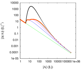
For the physical case with the twice iterated OPE reproduces closely the non-perturbative results. Because of this we consider the unphysical larger value111This value is chosen to reproduce the physical scattering length fm from the LS equation and the case. and show in Fig. 1 the comparison of the LHC discontinuity including (green), (blue), (magenta), (light blue), the result of Eq. (9) (red points) and the asymptotic expression Eq. (10) (black points), which is only taken for . In this case the contributions up to 4 pion exchanges are sizable.
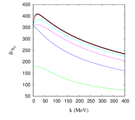
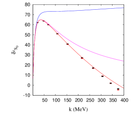
Now that we have the contribution to the LHC discontinuity of the iterated OPE to any order, we can use the method to calculate the partial-wave amplitude along the physical region (. As OPE in the singlet case is a regular interaction we can perform a regular calculation and compare with the result of the LS equation. As mentioned before, OPE in the partial wave is weak, and in order to see the effect of higher-order iterative diagrams in the calculation of we change the axial coupling constant to the unphysical value . The results for the phase-shifts are given in Fig. 2 where we can see that now the problem is non-perturbative; even including exchange is not enough to reproduce the phase shift. However with the solution of Eq. (9) we reproduce the calculation of the LS equation. Note that here we take the prescription of zero phase shift at infinite energy.222Levinson theorem, which is valid for regular interactions, implies that there are two bound states.
| (fm) | (fm) | (fm3) | ||
|---|---|---|---|---|
| -23.75 | 8.56 | 15.3 | ||
| -23.75 | 8.80 | 17.7 | ||
| N/D11 | -23.75 | 8.88 | 18.4 | |
| -23.75 | 8.90 | 18.6 | ||
| Non-perturbative | -23.75 | 8.90 | 18.7 | |
| 1.66 | 0.714 | -0.168 | ||
| 3.53 | 2.03 | -5.70 | ||
| N/D01 | 1.80 | 1.15 | -8.71 | |
| -6.89 | 13.7 | 47.5 | ||
| Non Perturbative | -23.75 | 8.90 | 18.7 |
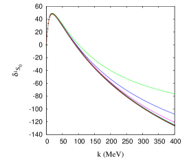
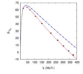
At this point it is interesting to check what we get if use the method with one subtraction fixing the scattering length to the value obtained from the LS equation. This is given in Fig 3 where we can see that if we include in the solution of Eq. (9) we recover exactly the result without subtractions. However in this case the contributions of the iterative diagrams to look perturbative and with exchange we almost recover the exact result. Note that here we take the prescription of zero phase shift at threshold.
In Table 1 we give the first three effective range parameters for both calculations, the regular one and the . For the latter the parameters vary slowly when more pion exchanges are added. For the regular solution, due to the fact that the system is highly non-perturbative, we do not see a convergent pattern, it will probably show up at a much higher order. However the final result in both prescriptions agrees.
These considerations show how a non-perturbative problem (with respect to the contributions from the LHC discontinuity to the physical partial-wave amplitude) is almost perturbative once one extra subtraction (or more) are taken.
We now compare the results given by the method with those of the LS equation renormalized with one counter term. We use three different regulators. The first one corresponds to a monopole form factor which gives the partial wave projection
| (11) |
where and has the same analytical properties as the OPE. The second and third ones are Gaussian type form factors
| (12) |
where and and have different analytical properties. In all cases for each value of we determine to reproduce the scattering length fm. We also calculate the LS equation using subtractive renormalization Frederico et al. (1999); Yang et al. (2009). It has the advantage that the counter term is removed from the equations and they depend explicitly on the low energy constant fixed, e.g. the scattering length .
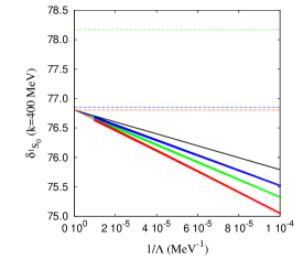
To compare with the result of the method we have to make an extrapolation to . In order to do that we plot in Fig. 4 the phase shift for MeV as a function of . In the Figure the dots represent the phase-shifts obtain with the LS equation with the counter terms introduced as in (red), (green) and (blue). These plots show a linear behavior and we make a linear fit to obtain the phase-shift at . The solid black line shows the result from subtractive renormalization Frederico et al. (1999); Yang et al. (2009). The dashed lines correspond to the results obtained from the case with the same colors as in Fig. 2. In this scale contributions from exchange can be observed. The final result agrees very well with the extrapolation made by the fit and this does not depend on the particular regulator used.
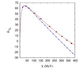
Finally, we give in Fig. 5 the phase shifts that result in the method with calculated from the LO ChPT potential. The cases , and are shown. The subtraction constants are fixed using fm, fm and fm3.
We now perform the method calculation with singular interactions given by the NLO and NNLO Chiral Effective Field Theory contributions Kaiser et al. (1997). At NNLO we use the LEC’s GeV-1, GeV-1 and GeV-1 obtained from the Roy-Steiner equations matched to ChPT Hoferichter et al. (2015). However, due to the singular character of the interaction not all the equations converge (contrary to the regular case of the Yukawa potential at LO). Indeed, since the interactions are singularly attractive one would expect no solution for the regular case and a well defined solution for the case, and this is what we obtain.333This expectation is based on the fact that a singularly attractive interaction requires to fix a constant relative phase Case (1950); Entem et al. (2008). The case does not converge, which explains from first principles why when trying to fix only and no solutions were obtained in the LS studies of Refs. Entem et al. (2008); Yang et al. (2009). The equations give a well defined result. Detailed discussions on the calculation of and about the convergence of different calculations will be given in a forthcoming paper Entem and Oller (forthcoming).
In Figs. 6 and 7 we show the results that stem from the calculations employing the NLO and NNLO ChPT potentials, respectively. We use the same values for , and and the same colors as in Fig. 5, additionally we also include as blue dots the result of subtractive renormalization.
In this work we did not perform a thorough fit of the phase shifts since the electromagnetic and charge symmetry breaking effects, which are important at low energies, has not been included yet. However, this work shows that the partial wave could be reproduced with good accuracy with the NNLO ChPT potential within the -case calculation.
A remarkably interesting feature of the method over the LS equation is that one can calculate straightforwardly the scattering amplitude in the whole -complex plane, once is known along the LHC, cf. Eq. (The method with non-perturbative left-hand-cut discontinuity and the partial wave). In this way, one could study directly the bound states, virtual states and resonances associated with the calculated partial-wave amplitude. The large scattering length in the partial wave is a signal of an antibound state. We can calculate the matrix in the second Riemann sheet [] using the analytical continuation of the first Riemann sheet given by
| (13) |
where is evaluated such that . So the antibound state is given by the zeros of . With one subtraction we obtain MeV at LO, and MeV for the NLO and NNLO cases. Using more than one subtraction we get MeV in all cases.
In summary, we have deduced for the first time in the literature an IE to obtain the full discontinuity of a partial-wave amplitude along the LHC, . This is then implemented within the method, with exact discontinuities both along the LHC and RHC. In this way, we obtain the equivalence between the method and the the LS equation for a Yukawa potential (regular potential). We also apply the method with the NLO and NNLO ChPT potentials, which are examples of singular attractive interactions Entem et al. (2008). The equivalence of the method with one extra subtraction and the LS equation renormalized with one counter term or with subtractive renormalization holds in this case as well. Within the method one can also include extra subtractions constants; we have done it up to three extra subtractions, which reproduces accurately the phase shifts of the Granada group analysis Pérez et al. (2013) when the NNLO ChPT potential is used. This goes definitely beyond the present nonperturbative solution of the LS equation in momentum space renormalized with counter terms, for which theoretical control in the regulator independent case is achieved only when taking one or none counter term Entem et al. (2008); Yang et al. (2009). Our results are far reaching and could be of great interest for atomic, molecular, nuclear and particle physics in which singular attractive potentials and short range interactions usually appear.
Acknowledgements.
This work has been partially funded by MINECO under Contract No. FPA2013-47443-C2-2-P, by the MINECO (Spain) and ERDF (European Commission) grant FPA2013-40483-P and by the Spanish Excellence Network on Hadronic Physics FIS2014-57026-REDT.References
- Weinberg (1990) S. Weinberg, Phys. Lett. B 251, 288 (1990).
- Weinberg (1991) S. Weinberg, Nucl. Phys. B 363, 3 (1991).
- Weinberg (1992) S. Weinberg, Phys. Lett. B 295, 114 (1992).
- Ordóñez et al. (1994) C. Ordóñez, L. Ray, and U. van Kolck, Phys. Rev. Lett. 72, 1982 (1994).
- Ordóñez et al. (1996) C. Ordóñez, L. Ray, and U. van Kolck, Phys. Rev. C 53, 2086 (1996).
- Kaiser et al. (1997) N. Kaiser, R. Brockmann, and W. Weise, Nucl. Phys. A 625, 758 (1997).
- Epelbaum et al. (1998) E. Epelbaum, W. Gloeckle, and U.-G. Meißner, Nucl. Phys. A 637, 107 (1998).
- Epelbaum et al. (2000) E. Epelbaum, W. Gloeckle, and U.-G. Meißner, Nucl. Phys. A 671, 295 (2000).
- Entem and Machleidt (2002) D. Entem and R. Machleidt, Phys. Lett. B 524, 93 (2002).
- Entem and Machleidt (2003) D. R. Entem and R. Machleidt, Phys. Rev. C 68, 041001 (2003).
- Epelbaum et al. (2015) E. Epelbaum, H. Krebs, and U.-G. Meißner, Phys. Rev. Lett. 115, 122301 (2015).
- Entem et al. (2015) D. R. Entem, N. Kaiser, R. Machleidt, and Y. Nosyk, Phys. Rev. C 92, 064001 (2015).
- Kaplan et al. (1998) D. B. Kaplan, M. J. Savage, and M. B. Wise, Phys. Lett. B 424, 390 (1998).
- Birse et al. (1999) M. C. Birse, J. A. McGovern, and K. G. Richardson, Phys. Lett. B 464, 169 (1999).
- Fleming et al. (2000) S. Fleming, T. Mehen, and I. W. Stewart, Nucl. Phys. A 677, 313 (2000).
- Oller (2003) J. A. Oller, Nucl. Phys. A 725, 85 (2003).
- Nieves (2003) J. Nieves, Physics Letters B 568, 109 (2003).
- Gegelia and Scherer (2006) J. Gegelia and S. Scherer, Int. J. Mod. Phys. A 21, 1079 (2006).
- Valderrama and Arriola (2004) M. P. Valderrama and E. R. Arriola, Phys. Lett. B 580, 149 (2004).
- Valderrama and Arriola (2005) M. P. Valderrama and E. R. Arriola, Phys. Rev. C 72, 054002 (2005).
- Harada et al. (2006) K. Harada, K. Inoue, and H. Kubo, Phys. Lett. B 636, 305 (2006).
- Nogga et al. (2005) A. Nogga, R. G. E. Timmermans, and U. v. Kolck, Phys. Rev. C 72, 054006 (2005).
- Valderrama and M. (2006) P. Valderrama and E. M., Ruiz Arriola, Phys. Rev. C 74, 054001 (2006).
- Mondejar and Soto (2007) J. Mondejar and J. Soto, Eur. Phys. J. A 32, 77 (2007).
- Pavón Valderrama (2011) M. Pavón Valderrama, Phys. Rev. C 83, 024003 (2011).
- Frederico et al. (1999) T. Frederico, V. Timóteo, and L. Tomio, Nucl. Phys. A 653, 209 (1999).
- Yang et al. (2009) C. J. Yang, C. Elster, and D. R. Phillips, Phys. Rev. C 80, 044002 (2009).
- Long and Yang (2012) B. Long and C.-J. Yang, Phys. Rev. C 85, 034002 (2012).
- Entem et al. (2008) D. R. Entem, E. R. Arriola, M. P. Valderrama, and R. Machleidt, Phys. Rev. C 77, 044006 (2008).
- Zeoli et al. (2013) C. Zeoli, R. Machleidt, and D. R. Entem, Few-Body Systems 54, 2191 (2013).
- Marji et al. (2013) E. Marji, A. Canul, Q. MacPherson, R. Winzer, C. Zeoli, D. R. Entem, and R. Machleidt, Phys. Rev. C 88, 054002 (2013).
- Behrendt et al. (2016) J. Behrendt, E. Epelbaum, J. Gegelia, U.-G. Meißner, and A. Nogga (2016), eprint 1606.01489.
- Chew and Mandelstam (1960) G. F. Chew and S. Mandelstam, Phys. Rev. 119, 467 (1960).
- Oller (2016) J. Oller, Phys. Rev. C 93, 024002 (2016).
- Guo et al. (2014) Z. Guo, J. Oller, and G. Ríos, Phys. Rev. C 89, 014002 (2014).
- Albaladejo and Oller (2012) M. Albaladejo and J. Oller, Phys. Rev. C 86, 034005 (2012).
- Albaladejo and Oller (2011) M. Albaladejo and J. Oller, Phys. Rev. C 84, 054009 (2011).
- Entem and Oller (forthcoming) D. R. Entem and J. A. Oller (forthcoming).
- Castillejo et al. (1956) L. Castillejo, R. H. Dalitz, and F. J. Dyson, Phys. Rev. 101, 453 (1956).
- Pérez et al. (2013) R. N. Pérez, J. E. Amaro, and E. R. Arriola, Phys. Rev. C 88, 064002 (2013).
- Stoks et al. (1993) V. G. J. Stoks, R. A. M. Klomp, M. C. M. Rentmeester, and J. J. de Swart, Phys. Rev. C 48, 792 (1993).
- Hoferichter et al. (2015) M. Hoferichter, J. Ruiz de Elvira, B. Kubis, and U.-G. Meißner, Phys. Rev. Lett. 115, 192301 (2015).
- Case (1950) K. Case, Phys. Rev. 80, 797 (1950).