Abstract

The $\gamma^{*}-f_{0}(980)$ transition form factors are calculated within the QCD factorization framework. The $f_{0}$-meson is assumed to be mainly generated through its $s\bar{s}$ Fock component. The corresponding spin wave function of the $f_{0}(980)$ meson is constructed and, combined with a model light-cone wave function for this Fock component, used in the calculation of the form factors. In the real-photon limit the results for the transverse form factor are compared to the large-momentum-transfer data measured by the BELLE collaboration recently. It turns out that, for the momentum-transfer range explored by BELLE, the collinear approximation does not suffice, power corrections to it, modeled as quark transverse moment effects, seem to be needed. Mixing of the $f_{0}$ with the $\sigma(500)$ is also briefly discussed.

1 Introduction

Recently the BELLE collaboration [1] has measured the cross section for $\gamma^{*}\gamma\to\pi^{0}\pi^{0}$ for large photon virtuality, $Q_{1}^{2}$, and small energy in the $\gamma^{*}\gamma$ center-of-mass system. From these data the photon-meson transition form factors have been extracted for the scalar, $f_{0}(980)$, and tensor, $f_{2}(1270)$, mesons for $Q_{1}^{2}\raisebox{-4.0pt}{$\,\stackrel{{\scriptstyle\textstyle<}}{{\sim}}\,$}30\,~{}{\rm GeV}^{2}$. These transition form factors are similar to those for the pseudoscalar mesons which have been extensively studied by both experimentalists and theoreticians. In Ref. [2] the $\gamma-f_{0}$ and the $\gamma-f_{2}$ form factors have been investigated within the NRQCD factorization framework [3], in which relativistic corrections and higher Fock state contributions are suppressed by powers of the relativistic velocity of the quarks in the meson, i.e. up to some minor modifications, the light mesons are treated like heavy Quarkonia. Super-convergence relations have been derived in [4] and shown to provide constraints on the $\gamma-f_{2}$ transition form factor. The latter form factor has also been studied within the framework of collinear factorization [5]. A phenomenological model for this form factor is discussed in [6]. The process $\gamma^{*}\gamma\to\pi\pi$ has been discussed in the framework of generalized distribution amplitudes, time-like versions of generalized parton distributions [7]. In this paper the interest is focused on the $\gamma-f_{0}$ transition form factor.

The $f_{0}(980)$ meson is a complicated system whose nature is not yet fully understood. Its peculiar properties have led to many speculations about its quark content. A comparison of the partial widths for the $f_{0}$ decays into pairs of pions and Kaons [8] under regard of the respective phase spaces reveals that the matrix element for $f_{0}\to K^{+}K^{-}$ is much larger than that for $f_{0}\to\pi^{+}\pi^{-}$. Thus, if the $f_{0}$ is viewed as a quark-antiquark state, it is dominantly an $s\bar{s}$ state. The comparison of the branching ratios for the radiative decays of the $\phi$-meson into the $f_{0}$ and $\pi^{0}$ leads to the same conclusion. However, the $f_{0}$-meson is not a pure $s\bar{s}$ state as is, for instance, obvious from the decay widths for $J/\Psi\to f_{0}\omega$ and $J/\Psi\to f_{0}\phi$. This fact is interpreted as $f_{0}-\sigma(500)$ mixing. Detailed phenomenological analyses of $f_{0}-\sigma$ mixing in various decay processes [9, 10, 11, 12] revealed two ranges for the mixing angle, $\varphi$,

$$(25-40)^{\circ}\hskip 43.36464pt(140-165)^{\circ}$$ (1)

A light scalar glueball may affect this result [9].

As an alternative to the quark-antiquark interpretation other authors [13, 14] have suggested a tetraquark configuration for the $f_{0}$-meson. This appears as a natural explanation for the fact that the $a_{0}(980)$ and the $f_{0}$ mesons are degenerate in mass and are the heaviest particles of the lightest scalar-meson nonet. For the tetraquark interpretation there seems to be no $f_{0}-\sigma$ mixing [11]. The drawback of this picture is that the two-pion decay of the $f_{0}$ is too small as compared to experiment whereas the $a_{0}\to\eta\pi$ is too large. In [15] it has been suggested that the lightest scalar-meson nonet, considered as tetraquarks states, mixes with the scalar-meson nonet with masses around 1200 MeV under the effect of the instanton force. The latter nonet is believed to have a predominant $q\bar{q}$ structure. This mixing leads to a better description of the light scalar-meson decays. The $f_{0}$ may also have a substantial $K\bar{K}$ molecule component [16]. It goes without saying that the real $f_{0}$-meson is a superposition of all these configurations.

The goal of the present paper is the calculation of the $\gamma^{*}-f_{0}$ transition form factors at large photon virtualities. For this calculation the pQCD framework developed by Brodsky and Lepage [17] is utilized in which the process is factorized in a perturbatively calculable hard subprocess (here $\gamma^{*}\gamma^{*}\to q\bar{q}$) and a soft hadronic matrix element, parametrized as a light-cone wave function, which is under control of soft, long-distance QCD. As any hadron the $f_{0}$-meson possesses a Fock decomposition [18] starting with the simple quark-antiquark components

$$|f_{0};p\rangle = \sum_{\beta}\int[d\tau]_{2}[d^{2}{\bf k}_{\perp}]_{2}\Psi_{2,\beta}(\tau,{\bf k}_{\perp})|q\bar{q},\beta;k_{1},k_{2}\rangle$$ (2)

$$+\;\textrm{higher Fock states}$$

where $\Psi_{2,\beta}$ is the light-cone wave function of the $q\bar{q}$ Fock state; the index $\beta$ labels its decomposition in flavor, color and helicity. The integration measures are defined by

$$[d\tau]_{2} = d\tau_{1}d\tau_{2}\,\delta(1-\tau_{1}-\tau_{2})\,,$$

$${[d^{2}{\bf k}_{\perp}]}_{2} = \frac{d^{2}{\bf k}_{\perp 1}d^{2}{\bf k}_{\perp 2}}{16\pi^{3}}\,\delta^{(2)}({\bf k}_{\perp 1}+{\bf k}_{\perp 2}-{\bf p}_{\perp})\,.$$ (3)

In the photon-photon interactions at large photon virtualities the $f_{0}$-meson is generated through its lowest Fock components, mainly the $s\bar{s}$ one. As can be shown [17] the hard generation of the $f_{0}$ through higher Fock components is suppressed by inverse powers of the photon virtuality and is therefore neglected. Once the meson is produced it gets dressed by fluctuations into higher Fock components under the effect of long-distance QCD. The calculation of the $\gamma^{*}-f_{0}$ transition form factors is similar to the one of the photon-pseudoscalar-meson form factors [17]. The latter calculation is to be generalized in such a way that also hadrons with non-zero orbital angular between their constituents can be treated.

The paper is organized as follows: In the next section the spin part of the light-cone wave function, termed the spin wave function, of the $f_{0}$ is constructed assuming that this mesons is an $s\bar{s}$ state. In Sect. 2.1 the collinear reduction of the spin wave function is discussed and, in Sect. 2.2, an example of a light-cone wave function of the $f_{0}$ is introduced and compared to the twist-2 and 3 distribution amplitudes. The $\gamma^{*}-f_{0}$ transition form factors are defined in Sect. 3.1, followed by a LO perturbative calculation within the modified perturbative approach in which quark transverse degrees of freedom are retained (Sect 3.2). Numerical results for the form factors in the real-photon limit are given in Sect. 4.1 and compared to the BELLE data. Some comments on the behavior of the $\gamma^{*}-f_{0}$ form factors are presented in Sect. 4.2. Finally, the summary will be given in Sect. 5.

2 The spin wave function of the $f_{0}$-meson

For the description of the hadron the light-cone approach is used which enables one to completely separate the dynamical and kinematical features of the Poincaré invariance [19, 20]. The overall motion of the hadron is decoupled from the internal motion of the constituents, i.e. the light-cone wave function of the hadron, $\Psi$, is independent of the hadron’s momentum and is invariant under the kinematical Poincaré transformations ( boosts along and rotations around the 3-directions as well as transverse boosts). Hence, $\Psi$ is determined if it is known at rest. The $s\bar{s}$ Fock component given in (2), is split in a spin part (hereafter denoted as spin wave function) and a reduced light-cone wave function, $\Psi_{0}$, which represents the full, soft wave function, $\Psi$, with a factor $K^{\mu}$ removed from it. As discussed in detail in Ref. [21] the covariant spin wave function can be constructed starting from the observation [22] that, in zero binding energy approximation, an equal-time hadron state (in the spin basis) in the constituent center-of-mass frame equals the (helicity) light-cone state at rest. Consequently, one can use the standard $ls$ coupling scheme in order to couple quark and antiquark to a state of given spin and parity. On boosting the results to a frame with arbitrary hadron momentum one easily reads off the covariant spin wave function .

Since the $f_{0}(980)$-meson is a $J^{PC}=0^{++}$ state the quark and antiquark have to couple in a spin-1 state and one unit of orbital angular momenta is required . The $ls$ coupling scheme leads to the following ansatz for the spin wave function of a final state meson in its rest frame [21, 23] ($\bar{S}_{0}=\gamma_{0}S^{\dagger}\gamma_{0}$)

$$\bar{S}_{0}\,=\,\sum_{m,\mu_{1},\mu_{2}}k\sqrt{4\pi}Y^{*}_{1m}({\bf k}/k)\left({1/2\atop\mu_{1}}{1/2\atop\mu_{2}}\left|{1\atop\mu_{s}}\right)\right.\left({1\atop\mu_{s}}{1\atop m}\left|{0_{\phantom{s}}\atop 0_{\phantom{s}}}\right)\right.v(\hat{p}_{2},\mu_{2})\bar{u}(\hat{p}_{1},\mu_{1})\,.$$ (4)

Note that $\mu_{1},\mu_{2}$ denote spin components and $v,\bar{u}$ are equal-t spinors here. In the meson’s rest frame the meson and the constituent momenta read

$$\hat{p}^{\mu}\,=\,(M_{0},{\bf 0})\,,\qquad\hat{p}_{1}^{\mu}\,=\,(m_{1},{\bf k})\,,\qquad\hat{p}_{2}^{\mu}\,=\,(m_{2},-{\bf k})\,.$$ (5)

where ${\bf k}$ is the three-momentum part of the relative momentum of quark and antiquark

$${\bf k}\,=\,\frac{1}{2}\big{(}\hat{{\bf p}}_{1}-\hat{{\bf p}}_{2}\big{)}\,.$$ (6)

In order to retain a covariant formulation, the four-vector $K=(0,{\bf k})$ is introduced . As is customary in the parton model, the binding energy is neglected and the constituents are considered as quasi on-shell particles. That possibly crude approximation can be achieved by putting the minus components of the constituents to zero. Hence, $k_{3}=0$ and our relative vector reduces to

$$K\,=\,\big{[}0\,0\,{\bf k}_{\perp}\big{]}\,.$$ (7)

In this case the spin wave function (4) reads

$$\bar{S}_{0}\,=\,\frac{1}{\sqrt{2}}\Big{[}k_{\perp+}v(\hat{p}_{2},+)\bar{u}(\hat{p}_{1},+)-k_{\perp-}v(\hat{p}_{2},-)\bar{u}(\hat{p}_{1},-)\Big{]}$$ (8)

where $k_{\perp\pm}=k_{\perp 1}\pm ik_{\perp 2}$. This spin wave function is of the same type as is discussed in [24] for the $l=1$ Fock components of $\rho$ and $\pi$-mesons.

In the infinite momentum frame (IMF), obtained by boosting the meson rest frame momenta along the 3-direction, $p\cdot K=0$ holds and the quark and antiquark momenta are parametrized as 

$$p_{1}\,=\,\tau p+K\,,\qquad p_{2}\,=\,\bar{\tau}p-K$$ (9)

where $\bar{\tau}=1-\tau$ and

$$p_{1}^{2}\,=\,m_{1}^{2}\,=\,\tau^{2}M_{0}^{2}+{\cal O}(k^{2}_{\perp})\,,\qquad p_{2}^{2}\,=\,m_{2}^{2}\,=\,\bar{\tau}^{2}M_{0}^{2}+{\cal O}(k^{2}_{\perp})\,.$$ (10)

The boost to the IMF leads to:

$$\bar{S}_{0}\,=\,\frac{1}{\sqrt{2}}\Big{[}\frac{2\xi}{1-\xi^{2}}\frac{k^{2}_{\perp}}{M_{0}}p\,/-2\frac{k^{2}_{\perp}}{1-\xi^{2}}+i\sigma^{\mu\nu}p_{\mu}K_{\nu}+M_{0}K/\Big{]}\,.$$ (11)

For convenience the variable $\xi=1-2\tau$ is introduced. For $\xi=0$ this covariant spin wave function coincides with the one employed for the $\chi_{c0}$ in [26]. The normalization of the spin wave function is chosen such that

$${\rm Tr}\Big{(}S_{0}^{\dagger}S_{0}\Big{)}\,=\,4E^{2}k^{2}_{\perp}+{\cal O}(k^{4}_{\perp})$$ (12)

where $E$ is the meson’s energy. The meson’s $s\bar{s}$ Fock state (2) explicitly reads

$$\langle f_{0};p|\,=\,\frac{\delta_{c\bar{c}}}{2\sqrt{N_{c}}}\int\frac{d\xi d^{2}k_{\perp}}{16\pi^{3}}\Psi_{0}(\xi,k^{2}_{\perp})\bar{S}_{0}\langle s_{c};p_{1},\lambda_{1}|\langle\bar{s}_{\bar{c}};p_{2},\lambda_{1}|\,,$$ (13)

The number of colors is denoted by $N_{c}$ and $c,\bar{c}$ are color labels. Proper state normalization requires the condition

$$\frac{1}{2}\int\frac{d\xi d^{2}k_{\perp}}{16\pi^{3}}k^{2}_{\perp}|\Psi_{0}(\tau,k^{2}_{\perp})|^{2}=P_{f_{0}}\leq 1$$ (14)

where $P_{f_{0}}$ is the probability of the $s\bar{s}$ Fock component.

2.1 Collinear reduction

In collinear approximation the limit $k_{\perp}\to 0$ in the hard subprocess is to be taken in general. However, terms $\propto K^{\alpha}$ in it combine with terms linear in $K$ in the spin wave function and therefore survive the $k_{\perp}$-integration of the wave function. These terms are in general of the same order as the other terms in the spin wave function and it is therefore unjustified to neglect these terms . Consider the expansion of the subprocess amplitude with respect to $K$:

$${\cal M}\,=\,A_{0}(\xi)+K^{\alpha}A_{1\alpha}(\xi)+{\cal O}(K^{\alpha}K^{\beta})$$ (15)

where $A_{0}$ is of order 1 while $A_{1}$ is of order $1/p^{+}$ for dimensional reason. The $k_{\perp}$-integration yields

$$\int\frac{d^{2}k_{\perp}}{16\pi^{3}}\Psi_{0}(\xi,k^{2}_{\perp})K/\,{\cal M}\,=\,-\frac{1}{2}g_{\perp}^{\nu\alpha}\gamma_{\nu}A_{1\alpha}\int\frac{dk^{2}_{\perp}}{16\pi^{2}}k^{2}_{\perp}\Psi_{0}\,.$$ (16)

Formally this is equivalent to the replacement

$$K/\Longrightarrow-\frac{k^{2}_{\perp}}{2}g_{\perp}^{\nu\alpha}\gamma_{\nu}\frac{\partial}{\partial K_{\nu}}\Big{|}_{K\to 0}\,.$$ (17)

The transverse metric tensor is defined by $g_{\perp}^{11}=g_{\perp}^{22}=-1$ while all other components are zero in a frame where the meson moves along the 3-direction. In the collinear limit the spin wave function becomes

$$\bar{S}_{0}^{\rm coll}\,=\,\frac{k^{2}_{\perp}}{\sqrt{2}}\,\Big{[}\frac{2\xi}{1-\xi^{2}}\frac{p\,/}{M_{0}}-\frac{2}{1-\xi^{2}}-\frac{1}{2}\big{(}i\sigma_{\mu\alpha}p^{\mu}+M_{0}\gamma_{\alpha}\big{)}g_{\perp}^{\alpha\beta}\frac{\partial}{\partial K_{\beta}}\,\Big{]}_{K\to 0}\,.$$ (18)

Multiplying the spin wave function with the reduced wave function and integrating over $k_{\perp}$, one arrives at the associated distribution amplitudes. The first term in (18) generates the twist-2 distribution amplitude

$$\frac{\bar{f}_{0}}{2\sqrt{2N_{c}}}\Phi_{0}(\xi)\,=\,\frac{2\xi}{1-\xi^{2}}\int\frac{dk_{\perp}^{2}}{16\pi^{2}}\,\frac{k^{2}_{\perp}}{M_{0}}\,\Psi_{0}\,.$$ (19)

Because of charge conjugation invariance the twist-2 distribution amplitude is antisymmetric in $\xi$. It possesses a Gegenbauer expansion and depends on the factorization scale, $\mu_{F}$, [10, 27, 28]

$$\Phi_{0}(\xi,\mu_{F})\,=\,\frac{N_{c}}{2}(1-\xi^{2})\sum_{m=1,3,\dots}B_{m}(\mu_{F})C_{m}^{3/2}(\xi)$$ (20)

Evidently, the reduced wave function must be symmetric in $\xi$. The Gegenbauer coefficients in (20) which encode the soft, non-perturbative QCD, evolve with the factorization scale as

$$B_{m}(\mu_{F})\,=\,B_{m}(\mu_{0})\left(\frac{\alpha_{\rm s}(\mu_{0})}{\alpha_{\rm s}(\mu_{F})}\right)^{-\gamma_{m}/\beta_{0}}$$ (21)

where

$$\gamma_{m}\,=\,C_{F}\Big{(}1-\frac{2}{(m+1)(m+2)}+4\sum_{j=2}^{m+1}\frac{1}{j}\Big{)}\,.$$ (22)

Here, $\beta_{0}=(11N_{c}-2n_{f})/3$, $C_{F}=4/3$ and $n_{f}$ denotes the number of active flavors. For the initial scale, $\mu_{0}$, the value $1.41\,~{}{\rm GeV}$ is chosen in this article. The decay constant $\bar{f}_{0}$ depends on the scale too [10]

$$\bar{f}_{0}(\mu_{F})\,=\,\bar{f}_{0}(\mu_{0})\left(\frac{\alpha_{\rm s}(\mu_{0})}{\alpha_{\rm s}(\mu_{F})}\right)^{4/\beta_{0}}\,.$$ (23)

The other terms in (18) are of twist-3 nature although they do not correspond to the full twist-3 contributions since, in general, they also receive contributions from a second reduced wave function. This is however of no relevance for the purpose of the present paper, namely the calculation of the $\gamma^{*}-f_{0}$ transition form factors. As we shall see in the following there is no twist-3 contribution to it. Anyway the $k_{\perp}$-integration of the other terms leads to two further distribution amplitudes which are related to $\Phi_{0}$ in the case at hand:

$$\Phi_{0s}(\xi,\mu_{F})\,=\,\frac{1}{\xi}\Phi_{0}(\xi,\mu_{F})\,,\qquad\Phi_{0\sigma}(\xi,\mu_{F})\,=\,\frac{1-\xi^{2}}{4\xi}\Phi_{0}(\xi,\mu_{F})\,.$$ (24)

Both these distribution amplitudes are symmetric in $\xi$ and only the even terms appear in their Gegenbauer expansions.

With the help of these distribution amplitudes one can transform the product of wave function and collinear spin wave function (18), integrated over $k_{\perp}$, into the form

$$\int\frac{d^{2}k_{\perp}}{16\pi^{3}}\Psi_{0}(\xi,k^{2}_{\perp})\bar{S}_{0}^{\rm coll} = \frac{\bar{f}_{0}}{2\sqrt{2N_{c}}}\frac{1}{\sqrt{2}}\Big{[}\Phi_{0}p\,/\,-\Phi_{0s}M_{0}$$ (25)

$$- \Phi_{0\sigma}M_{0}(i\sigma_{\mu\alpha}p^{\mu}+M_{0}\gamma_{\alpha})\;\,g_{\perp}^{\alpha\beta}\frac{\partial}{\partial K_{\beta}}\Big{]}_{K\to 0}\,.$$

This expression resembles the corresponding pion spin wave function to twist-3 accuracy [29, 30].

2.2 A wave function for the $f_{0}$ meson

For the evaluation of the transition form factors the light-cone wave function is to be specified. It is modeled as a Gaussian in $k^{2}_{\perp}/(1-\xi^{2})$ times the most general $\xi$ dependence

$$\Psi_{0}\,=\,c\sum_{n=0,2\ldots}\tilde{B}_{n}C_{n}^{3/2}(\xi)\exp{[-4\frac{a_{0}^{2}k_{\perp}^{2}}{1-\xi^{2}}]}$$ (26)

with

$$c\,=\,16\pi^{2}\sqrt{2N_{c}}\bar{f}_{0}M_{0}a_{0}^{4}\,.$$ (27)

This wave function is similar to the one for the pion advocated for in [18]. It has been used for instance in the calculation of the photon-pseudoscalar transition form factors [31] or in the analysis of pion electroproduction [32]. Insertion of the wave function into Eq. (19) leads to the associated distribution amplitude (20) with the Gegenbauer coefficients ($m$ is an odd integer)

$$B_{m}\,=\,\frac{m}{2m+1}\tilde{B}_{m-1}+\frac{m+3}{2m+5}\tilde{B}_{m+1}\,.$$ (28)

As a consequence of charge conjugation invariance which forces $\Psi_{0}$ to be symmetric in $\xi$, the matrix element

$$\langle f_{0};p|\bar{s}(0)\gamma_{\mu}s(0)|0\rangle\,=\,\frac{\sqrt{N_{c}}}{2}\int d\xi\frac{dk^{2}_{\perp}}{16\pi^{2}}\Psi_{0}{\rm Tr}\big{[}\bar{S}_{0}\gamma_{\mu}\big{]}$$ (29)

vanishes in accord with the result quoted in [10]. On the other hand, the scalar density provides

$$\langle f_{0};p|\bar{s}(0)s(0)|0\rangle\,=\,M_{0}\bar{f}_{0}\,=\,\frac{\sqrt{N_{c}}}{2}\int d\xi\frac{dk^{2}_{\perp}}{16\pi^{2}}\Psi_{0}{\rm Tr}\big{[}\bar{S}_{0}\big{]}\,.$$ (30)

Evaluation of the integral leads to $\tilde{B}_{0}\simeq-1$. This estimate is to be taken with caution since $\Phi_{0s}$ in (24) is likely not the full twist-3 distribution amplitude, but it provides orientation. As is obvious from the vacuum-particle matrix element of quark field operators given in (30), the decay constant is a short-distance quantity; it represents the wave function at the origin of the configuration space. It is also clear that only the $s\bar{s}$ Fock component of the $f_{0}$-meson contributes to this matrix element.

For the numerical evaluation of the $\gamma^{*}-f_{0}$ transition form factors the wave function will be restricted to the first Gegenbauer term, all others are neglected.

$$\Psi_{01}\,=\,3cB_{1}\exp{[-4\frac{a_{0}^{2}k_{\perp}^{2}}{1-\xi^{2}}]}$$ (31)

with

$$B_{1}\simeq\tilde{B}_{0}/3\simeq-1/3\,.$$ (32)

In this case the twist-2 distribution amplitude reads

$$\Phi_{01}\,=\,\frac{N_{c}}{2}(1-\xi^{2})B_{1}C_{1}^{3/2}(\xi)\,.$$ (33)

For the transverse-size parameter, $a_{0}$, the value $0.8\,~{}{\rm GeV}^{-1}$ is taken in the following. This value is very close to the corresponding value for the pion, see [31]. The r.m.s. $k_{\perp}$ is related to the transverse-size parameter by

$$\sqrt{\langle k^{2}_{\perp}\rangle}\,=\,\sqrt{\frac{3}{14}}\,\frac{1}{a_{0}}\,.$$ (34)

For the value $a_{0}=0.8\,~{}{\rm GeV}^{-1}$ the r.m.s. value of $k_{\perp}$ is $0.58\,~{}{\rm GeV}$ which is similar to the corresponding results for the valence Fock components of other hadrons. For the decay constant the value

$$\bar{f}_{0}(\mu_{0})=(180\pm 15)\,~{}{\rm MeV}$$ (35)

is adopted which has been derived by De Fazio and Pennington [33] from radiative $\phi\to f_{0}\gamma$ decays with the help of QCD sum rules (see also [34]). In [33] the $f_{0}$-meson is considered as a (dominantly) $s\bar{s}$ state. The value (35) is extracted from the stability window for the Borel parameter between 1.2 and $2\,~{}{\rm GeV}^{2}$. This is consistent with the initial scale chosen in this article.

3 The $\gamma^{*}-f_{0}$ transition form factors

3.1 The definition of the form factors

Let us consider the general case of two virtual photons

$$\gamma^{*}(q_{1},\lambda_{1})+\gamma^{*}(q_{2},\lambda_{2})\to f_{0}(p)$$ (36)

where $q_{i}$ and $p$ denote the momenta of the photons and the mesons while $\lambda_{i}$ are the helicities of the photons. One has

$$q_{1}^{2}\,=\,-Q_{1}^{2}\,,\qquad q_{2}^{2}\,=\,-Q_{2}^{2}\,,\qquad p^{2}=M_{0}^{2}\,.$$ (37)

It is convenient to introduce the following variables [35]

$$\overline{Q}^{2}\,=\,\frac{1}{2}(Q_{1}^{2}+Q^{2}_{2})\,,\qquad\omega\,=\,\frac{Q^{2}_{1}-Q^{2}_{2}}{Q^{2}_{1}+Q^{2}_{2}}$$ (38)

where, obviously, $-1\leq\omega\leq 1$.

The transition vertex is defined by the matrix element of the time-ordered product of two electromagnetic currents

$$\Gamma^{\mu\nu}\,=\,-ie_{0}^{2}\int d^{4}xe^{-iq_{1}x}\langle f_{0};p\mid T\{j^{\mu}_{\rm em}(x)j^{\nu}_{\rm em}(0)\}\mid 0\rangle$$ (39)

where

$$j^{\mu}_{\rm em}\,=\,e_{u}\bar{u}(x)\gamma^{\mu}u(x)+e_{d}\bar{d}(x)\gamma^{\mu}d(x)+e_{s}\bar{s}(x)\gamma^{\mu}s(x)$$ (40)

and $e_{i}$ are the quark charges in units of the positron charge, $e_{0}$. Following [4] the vertex is covariantly decomposed as

$$\Gamma^{\mu\nu} = ie_{0}^{2}\frac{q_{1}\cdot q_{2}}{M_{0}}\left\{\Big{[}-g^{\mu\nu}+\frac{1}{\overline{Q}^{4}\kappa}\big{[}q_{1}\cdot q_{2}(q_{1}^{\mu}q_{2}^{\nu}+q_{2}^{\mu}q_{1}^{\nu})\right.$$ (41)

$$\left.\hskip 65.04034pt+\,Q_{1}^{2}q_{2}^{\mu}q_{2}^{\nu}+Q_{2}^{2}q_{1}^{\mu}q_{1}^{\nu}\big{)}\big{]}\Big{]}\,F_{T}(\overline{Q}^{2},\omega)\right.$$

$$- \left.\frac{q_{1}\cdot q_{2}}{\overline{Q}^{4}\kappa}\Big{[}q_{1}^{\mu}+\frac{Q_{1}^{2}}{q_{1}\cdot q_{2}}q_{2}^{\mu}\Big{]}\Big{[}q_{2}^{\nu}+\frac{Q_{2}^{2}}{q_{1}\cdot q_{2}}q_{1}^{\nu}\Big{]}\,F_{L}(\overline{Q}^{2},\omega)\right\}$$

where

$$\kappa\,=\,\frac{(q_{1}\cdot q_{2})^{2}}{\overline{Q}^{4}}-1+\omega^{2}\,=\,\omega^{2}+\frac{M_{0}^{2}}{\overline{Q}^{2}}+\frac{M_{0}^{4}}{4\overline{Q}^{4}}\,.$$ (42)

Current conversation is manifest:

$$q_{1\mu}\Gamma^{\mu\nu}\,=\,0\,,\qquad q_{2\nu}\Gamma^{\mu\nu}\,=\,0\,.$$ (43)

As one sees from (41) there are two form factors, one for transverse photon polarization, $F_{T}$, and another one for longitudinal polarization, $F_{L}$. By definition the form factors are dimensionless.

Contracting the vertex function with the polarization vectors of the photons and using transversality ($\epsilon_{i}q_{i}=0$), one arrives at

$$\epsilon_{1}^{\mu}\epsilon_{2}^{\nu}\Gamma_{\mu\nu} = ie_{0}^{2}\frac{q_{1}\cdot q_{2}}{M_{0}}\left\{\Big{[}-\epsilon_{1}\cdot\epsilon_{2}+\frac{q_{1}\cdot q_{2}}{\kappa\overline{Q}^{4}}\epsilon_{1}\cdot q_{2}\epsilon_{2}\cdot q_{1}\Big{]}\,F_{T}\right.$$ (44)

$$\left.\hskip 43.36464pt-\frac{1-\omega^{2}}{\kappa q_{1}\cdot q_{2}}\epsilon_{1}\cdot q_{2}\epsilon_{2}\cdot q_{1}\,F_{L}\right\}\,.$$

One can show, most easily in the equal-energy brick wall frame (see Fig. 1), defined by

$$q_{1}\,=\,(\nu\,0\,0\,a_{1})\,,\qquad q_{2}\,=\,(\nu\,0\,0\,a_{2})\,,\qquad p\,=\,(2\nu\,0\,0\,a_{1}+a_{2})\,,$$ (45)

that the contraction with transverse photon polarization vectors with the same helicity projects out the form factor $F_{T}$ and with longitudinal ones $F_{L}$:

$$\epsilon_{1}^{\mu}(\lambda_{1})\epsilon_{2}^{\nu}(\lambda_{2})\Gamma_{\mu\nu} = -ie_{0}^{2}\frac{q_{1}\cdot q_{2}}{M_{0}}F_{T}(\overline{Q}^{2},\omega)\delta_{\lambda_{1}\lambda_{2}}\,,$$

$$\epsilon_{1}^{\mu}(0)\epsilon_{2}^{\nu}(0)\Gamma_{\mu\nu} = \phantom{-}ie_{0}^{2}\sqrt{1-\omega^{2}}\frac{\overline{Q}^{2}}{M_{0}}F_{L}(\overline{Q}^{2},\omega)\,.$$ (46)

If the photons have different helicities the vertex function is zero.

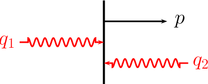
Figure 1: The equal-energy brick wall frame.

3.2 The LO perturbative calculation

In the perturbative calculation of the form factors, performed at large $\overline{Q}^{2}$, the mass of the $f_{0}$-meson is neglected whenever this is possible. From the Feynman graphs shown in Fig. 2 one finds for the vertex function (39)

$$\Gamma_{\mu\nu} = -i\frac{1}{2}e_{0}^{2}e_{s}^{2}\sqrt{N_{c}}\int\frac{d\xi d^{2}k_{\perp}}{16\pi^{3}}\Psi_{0}(\xi,k_{\perp})\left\{{\rm Tr}\Big{[}\bar{S}_{0}\,\gamma_{\mu}\frac{\frac{1}{2}(1-\xi)p\,/+K/-q_{1}\,/}{g_{1}^{2}}\,\gamma_{\nu}\Big{]}\right.$$ (47)

$$\left.\hskip 108.405pt+{\rm Tr}\Big{[}\bar{S}_{0}\,\gamma_{\nu}\frac{\frac{1}{2}(1-\xi)p\,/+K/-q_{2}\,/}{g_{2}^{2}}\,\gamma_{\mu}\Big{]}\right\}$$

where the parton virtualities read (see also Fig. 2)

$$g_{1}^{2}\,=\,-\overline{Q}^{2}(1+\xi\omega)-k_{\perp}^{2}\,,\qquad g_{2}^{2}\,=\,-\overline{Q}^{2}(1-\xi\omega)-k_{\perp}^{2}\,.$$ (48)

Taking into consideration that the traces are only non-zero for even numbers of $\gamma$ matrices, one notices that only the first term of the spin wave function (11), i.e. the leading-twist piece, contributes to the traces. The twist-3 terms lead to an odd number of $\gamma$ matrices in the traces, the fourth term is neglected. With the help of (46) one finally arrives at the following expressions for the form factors:

$$F_{T}(\overline{Q}^{2},\omega) = -4\sqrt{2N_{c}}\frac{e_{s}^{2}}{\overline{Q}^{2}}\frac{\omega^{2}+\frac{1}{2}\frac{M_{0}^{2}}{\overline{Q}^{2}}}{1+\frac{1}{2}\frac{M_{0}^{2}}{\overline{Q}^{2}}}\int\frac{d\xi dk^{2}_{\perp}}{16\pi^{2}}k^{2}_{\perp}\Psi_{0}(\xi,k_{\perp})\frac{\xi^{2}}{1-\xi^{2}}\,$$

$$\hskip 108.405pt\times\frac{1}{1-\xi^{2}\omega^{2}+2k^{2}_{\perp}/\overline{Q}^{2}}\,,$$

$$F_{L}(\overline{Q}^{2},\omega) = -\frac{1}{2}\frac{M_{0}^{2}}{\overline{Q}^{2}}\frac{1+\frac{1}{2}\frac{M_{0}^{2}}{\overline{Q}^{2}}}{\omega^{2}+\frac{1}{2}\frac{M_{0}^{2}}{\overline{Q}^{2}}}F_{T}(\overline{Q}^{2},\omega)\,.$$ (49)

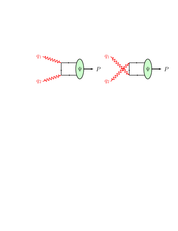
Figure 2: LO Feynman graphs for the $\gamma^{*}\to f_{0}$ transition form factors. The momenta of the virtual partons are denoted by $g_{1}$ and $g_{2}$.

Because of the variation of $\omega^{2}$ between 0 and 1 the mass dependent terms in front of the integral are kept. For $\omega\to\pm 1$ they exactly cancel whereas for $\omega\to 0$ $F_{T}\propto\overline{Q}^{-4}$. The wave function (26) generates a factor $(1-\xi^{2})^{2}$ in the $k^{2}_{\perp}$ integration. Hence, there is no singularity at the end points $\xi\to\pm 1$ for all $\omega$. One also notices from (49) that

$$F_{T,L}(\overline{Q}^{2},-\omega)\,=\,F_{T,L}(\overline{Q}^{2},\omega)\,.$$ (50)

For $\omega\gg M_{0}^{2}/(2\overline{Q}^{2})$ the terms $\sim M_{0}^{2}/\overline{Q}^{2}$ in (49) can be neglected and

$$F_{T}\propto 1/\overline{Q}^{2}\,,\qquad F_{L}\propto 1/\overline{Q}^{4}\,.$$ (51)

For $\omega\to 0$, on the other hand, only the term $\sim M_{0}^{2}/(2\overline{Q}^{2})$ remains and

$$F_{T,L}\propto 1/\overline{Q}^{4}\,.$$ (52)

Explicitly, for $\omega\to 1$ (i.e. $Q_{2}^{2}=0$)

$$F_{T}(Q_{1}^{2},1) = -8\sqrt{2N_{c}}\frac{e_{s}^{2}}{Q_{1}^{2}}\int\frac{d\xi dk^{2}_{\perp}}{16\pi^{2}}k^{2}_{\perp}\Psi_{0}(\xi,k_{\perp})$$ (53)

$$\times \frac{\xi^{2}}{1-\xi^{2}}\,\frac{1}{1-\xi^{2}+4k^{2}_{\perp}/Q_{1}^{2}}\,.$$

Figure 3: The reduction function $\varrho$ versus $a_{0}^{2}Q_{1}^{2}$.

For a wave function of the type (26) one can write Eq. (53) as

$$F_{T}(Q_{1}^{2},1)\,=\,\varrho(a_{0}^{2}Q_{1}^{2})\,F_{T}^{\rm coll}(Q_{1}^{2},1)$$ (54)

with

$$F_{T}^{\rm coll} = -2\frac{e_{s}^{2}}{Q_{1}^{2}}\bar{f}_{0}M_{0}\int d\xi\frac{\xi\Phi_{0}(\xi)}{1-\xi^{2}}$$ (55)

$$= -2N_{c}\frac{e_{s}^{2}}{Q_{1}^{2}}\bar{f}_{0}M_{0}\sum_{m=1,3\ldots}B_{m}$$

and

$$\varrho(x)\,=\,\int dK\frac{Ke^{-K}}{1+K/x}\,.$$ (56)

For this type of wave functions the transition form factor is given by the collinear result multiplied by a universal reduction factor $\varrho$. The latter function is shown in Fig. 3. It is interesting that, in the collinear approximation, the LO perturbative result for the form factor is related to the sum over all Gegenbauer coefficients. The $\gamma-\pi$ transition form factor possesses this property too. This makes it clear that it is impossible to extract more than one Gegenbauer coefficient from the $\gamma-f_{0}$ transition form factor data. This coefficient is to be regarded as an effective one. NLO corrections may allow one to fix a second coefficient [35]. The situation improves for $|\omega|<1$ as will be discussed in Sect. 4.2.

4 Results

4.1 The real-photon limit

The BELLE collaboration [1] extracted the $\gamma-f_{0}$ transition form factor from the cross sections on $\gamma^{*}\gamma\to\pi^{0}\pi^{0}$. In order to fix the normalization of that form factor the couplings of the $f_{0}$ to both the two-photon and the $\pi\pi$ channels are required. Both these couplings are not well known [8]. Hence, the normalization of the $\gamma-f_{0}$ transition form factor is subject to considerable uncertainties. The published data on the transition form factor, $F_{T}(Q_{1}^{2})$, are scaled by the value of the form factor at $Q_{1}^{2}=0$ obtained from the width of the two-photon decay of the $f_{0}$-meson ($M_{0}=(990\pm 20)\,~{}{\rm MeV}$ [8])

$$\Gamma(f_{0}\to\gamma\gamma)\,=\,\frac{\pi}{4}\alpha_{\rm em}^{2}M_{0}|F_{T}(0)|^{2}\,.$$ (57)

From the average decay width quoted in [8], one obtains

$$|F_{T}(0)|\,=\,0.0865\pm 0.0141\,.$$ (58)

The BELLE collaboration uses the slightly different value $|F_{T}(0)|_{\rm BELLE}\,=\,0.0832\pm 0.0136$.

In a first step the BELLE data are compared to the collinear result (55) for $F_{T}$. For the factorization scale $\mu^{2}_{F}=Q_{1}^{2}$ is used and for $\Lambda_{\rm QCD}$ the value $180\,~{}{\rm MeV}$ in combination with four flavors. Allowing only for the first Gegenbauer term in the expansion (20) of $\Phi_{0}$ and taking for the decay constant the value (35), we fit $B_{1}$ against the BELLE data. The fit yields $B_{1}^{\rm coll}(\mu_{0})=-0.44\pm 0.04$ and $\chi^{2}=10.3$ for 9 data points. The fitted value of $B_{1}$ is not far from the estimate quoted in (32). For these wave function parameters the probability of the $s\bar{s}$ Fock component of the $f_{0}$-meson is (see(14)):

$$P_{f_{0}}\,=\,\frac{12}{5}N_{c}\big{[}\pi\bar{f}_{0}M_{0}a_{0}^{2}B_{1}\big{]}^{2}\,=\,0.18\,.$$ (59)

The results of the fit are shown in Fig. 4. Reasonable agreement with experiment is to be seen within rather large errors although the shape of the fit is opposite to that of the data: the collinear result for the scaled form factor, $Q_{1}^{2}F_{T}^{\rm coll}$ slightly decreases with increasing $Q_{1}$ due to the evolution of the decay constant and the Gegenbauer coefficient, $B_{1}$, whereas the data increase in tendency.

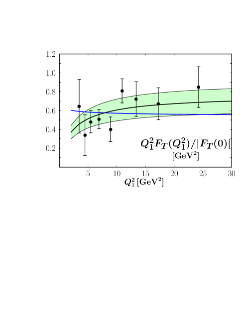
Figure 4: The $Q^{2}$-dependence of the $\gamma-f_{0}$ transition form factor scaled by $|F_{T}(0)|/Q_{1}^{2}$ (for $|F_{T}(0)|$ the value (58) is taken). Data are taken from [1]; only the statistical errors are shown. The dashed and solid lines are the results of the collinear approximation and the modified perturbative approach evaluated from wave function (31), respectively. The shaded band represents the normalization uncertainty of the second result.

An increasing scaled form factor can be generated by quark transverse momenta in the hard scattering kernel and in the wave function, see Fig. 3. Retaining the quark transverse momenta implies that quarks and antiquarks are pulled apart in the transverse configuration or impact-parameter space. The separation of color sources is accompanied by the radiation of gluons. These radiative corrections have been calculated in Ref. [36] in the form of a Sudakov factor in the impact parameter plane. The Sudakov factor, $e^{-S}$, comprises resummed leading and next-to-leading logarithms which are not taken into account by the usual QCD evolution. The $k_{\perp}$-factorization combined with the Sudakov factor is termed the modified perturbative approach (mpa)[36]. It has been used, for instance, in calculations of the pion electromagnetic form factor [36] or the $\pi-\gamma$ transition form factor [31] and will be used here as well. In the impact-parameter plane the transition form factor (53) reads

$$F_{T}(Q_{1}^{2},1) = -\frac{e_{s}^{2}\sqrt{2N_{C}}}{2\pi}\,\int_{-1}^{1}d\xi\frac{\xi^{2}}{1-\xi^{2}}$$ (60)

$$\times \int_{0}^{1/\Lambda_{\rm QCD}}dbb\Big{[}k_{\perp}^{2}\Psi_{0}\Big{]}\,e^{-S}K_{0}\Big{(}bQ_{1}/2\sqrt{1-\xi^{2}}\,\Big{)}\,.$$

The integrand is completed by the Sudakov factor, $\exp{(-S)}$, its explicit form can be found for instance in [31]. The Sudakov factor provides the sharp cut-off of the $b$-integral at $1/\Lambda_{\rm QCD}$. Since $1/b$ in the Sudakov factor marks the interface between the non-perturbative soft momenta which are implicitly accounted for in the meson wave function, and the contributions from soft gluons, incorporated in a perturbative way in the Sudakov factor [36, 31], it naturally acts as the factorization scale. The Bessel function $K_{0}$ is the Fourier transform of the hard scattering kernel and $\Big{[}k^{2}_{\perp}\Psi_{0}\Big{]}$ is the Fourier transform of the wave function (31) multiplied by $k^{2}_{\perp}$. It reads

$$\Big{[}k^{2}_{\perp}\Psi_{0}\Big{]} = \frac{3\pi}{4}\sqrt{2N_{C}}\bar{f}_{0}M_{0}B_{1}(1-\xi^{2})^{2}\Big{(}1-\frac{1-\xi^{2}}{16a_{0}^{2}}b^{2}\Big{)}e^{-\frac{1-\xi^{2}}{16a_{0}^{2}}b^{2}}\,.$$ (61)

Evaluating the form factor within the modified perturbative approach and fitting $B_{1}$ to the BELLE data [1] one arrives at the results shown in Fig. 4. The fit provides the following value for the Gegenbauer coefficient 

$$B_{1}^{\rm mpa}(\mu_{0})\,=\,-0.57\pm 0.05$$ (62)

and $\chi^{2}=5.9$ for 9 data points. The normalization uncertainty of the theoretical result follows from the errors of $B_{1}$ and $F_{T}(0)$, see (58). The agreement of the result obtained within the modified perturbative approach, with experiment is somewhat better than for the collinear approximation - the scaled form factor increases with $Q^{2}_{1}$ as the data do. This increase is the effect of the $k_{\perp}$ corrections shown in Fig. 3, the Sudakov factor plays a minor role in this context . In passing it is noted that the predictions presented in [2] lie markedly below experiment for $Q_{1}^{2}\raisebox{-4.0pt}{$\,\stackrel{{\scriptstyle\textstyle>}}{{\sim}}\,$}10\,~{}{\rm GeV}^{2}$.

The value (62) of the Gegenbauer coefficient $B_{1}$ is not far from the QCD sum result [10]:

$$\bar{f}_{0}(\mu_{0})\,=\,(410\pm 22)\,~{}{\rm MeV}\,,\qquad B_{1}(\mu_{0})\,=\,-0.65\pm 0.07\,.$$ (63)

The coefficent $B_{3}$ is found to be zero within errors. However, the value of $\bar{f}_{0}$ is substantially larger than the value (35) used in the form factor calculation. More precisely, the fit to the BELLE data fixes the product of $\bar{f}_{0}$ and $B_{1}$ for which the following results exist

$$\bar{f}_{0}(\mu_{0})B_{1}(\mu_{0}) = (-0.079\pm 0.007)\,~{}{\rm GeV}\hskip 43.36464pt{\rm collinear}$$ (64)

$$= (-0.103\pm 0.990)\,~{}{\rm GeV}\hskip 43.36464pt{\rm mpa}$$

$$= (-0.267\pm 0.029)\,~{}{\rm GeV}\hskip 43.36464pt\cite[cite]{[\@@bibref{}{cheng05}{}{}]}$$

The product of $\bar{f}_{0}$ and $B_{1}$ derived in [10] is substantially larger than the BELLE data [1] on the $\gamma-f_{0}$ transition form factors allow. This product of $\bar{f}_{0}$ and $B_{1}$ is also in conflict with a light-cone wave function interpretation since it leads to a probability larger than 1. Of course a smaller value of the transverse-size parameter would cure this problem for the prize of an implausible compact valence Fock component. For instance, if one halves $a_{0}$ the probability is about 0.12 but $\sqrt{\langle k^{2}_{\perp}\rangle}\simeq 1.2\,~{}{\rm GeV}$.

The last issue to be discussed is the contribution from the non-strange $q\bar{q}$ Fock state to the $\gamma-f_{0}$ transition form factor. This is usually considered as $f_{0}-\sigma$ mixing [9]-[15]. As for the $\eta-\eta^{\prime}$ system [37] this mixing is treated in the quark-flavor basis. As a consequence of the smallness of OZI-rule violations $\eta-\eta^{\prime}$ mixing is particularly simple in that basis - there is a common mixing angle for the states and the decay constants. It is assumed that this mixing scheme also holds for the case of interest here. Let $\sigma_{n}$ and $\sigma_{s}$ be states with the lowest Fock components $n\bar{n}=(u\bar{u}+d\bar{d})/\sqrt{2}$ and $s\bar{s}$, respectively. In analogy to (30) the corresponding decay constants are defined by the $\sigma_{i}$-vacuum matrix elements of the quark field operators:

$$\langle\sigma_{n}|\bar{n}(0)n(0)|0\rangle=M_{\sigma_{n}}\bar{f}_{n}\,,\qquad\langle\sigma_{s}|\bar{s}(0)s(0)|0\rangle=M_{\sigma_{s}}\bar{f}_{s}\,.$$ (65)

Since in hard processes only small spatial quark-antiquark separations are of relevance it seems plausible to embed the particle dependence and the mixing behavior of the $q\bar{q}$ Fock components solely into the decay constants  (for a detailed discussion of this procedure in the $\eta-\eta^{\prime}$ case see [38]). In generalization of (30) one may also define the decay constants $\bar{f}_{i}^{q}$ ($i=f_{0},\sigma$; $q=n,s$)

$$\langle i|\bar{q}(0)q(0)|0\rangle\,=\,M_{i}\bar{f}_{i}^{q}\,.$$ (66)

These decay constants mix according to

$$\bar{f}_{\sigma}^{n} = \bar{f}_{n}\cos{\varphi}\,,\qquad\bar{f}_{\sigma}^{s}\,=\,-\bar{f}_{s}\sin{\varphi}\,,$$

$$\bar{f}_{0}^{n} = \bar{f}_{n}\sin{\varphi}\,,\qquad\bar{f}_{0}^{s}\,=\,\phantom{-}\bar{f}_{s}\cos{\varphi}\,.$$ (67)

Hence, the $\gamma^{*}-f_{0}$ transition form factors are made of two contributions

$$F_{T,L}\,=\,F_{T,L}^{n}+F_{T,L}^{s}$$ (68)

where the $n$ and $s$ contributions differ from (49) only by the decay constants, $\bar{f}_{n}$ and $\bar{f}_{s}$, the mixing angle, $\varphi$, and the quark charges, $(e_{u}^{2}+e_{d}^{2})/\sqrt{2}$ and $e_{s}^{2}$. Thus, the contribution from the $n\bar{n}$ Fock state is taken into account if in (49), and in other expressions derived for the form factors, the decay constant, $\bar{f}_{0}$, is to be replaced by an effective one defined by

$$\bar{f}^{\rm eff}_{0}\,=\,\bar{f}_{n}\sin{\varphi}\frac{1}{\sqrt{2}}\frac{e_{u}^{2}+e_{d}^{2}}{e_{s}^{2}}+\bar{f}_{s}\cos{\varphi}\,.$$ (69)

According to [10, 39] $\bar{f}_{n}\simeq\bar{f}_{s}$. Since the decay constant quoted in (35) is to be identified with $\bar{f}_{0}^{s}$ and since $|\cos{\varphi}|$ is close to 1, see (1), it suffices to assume $\bar{f}_{n}\simeq\bar{f}_{s}\simeq\bar{f}_{0}$ for a rough estimate. For the range $\varphi=(25-40)^{\circ}$ of the mixing angle quoted in (1) one finds

$$\bar{f}^{\rm eff}_{0}/\bar{f}_{0}\,=\,2.4-3.0\,.$$ (70)

Clearly, this leads to a transition form factor which is in conflict with the BELLE data [1]. Using the second range of mixing angles in (1) one obtains reasonable agreement with experiment. Particularly favored is the range $\varphi=(145-151)^{\circ}$ for which the form factor stays within the uncertainty band displayed in Fig. 4. An exact determination of the mixing angle is not possible at present given the poor information available for the basic decay constants, $\bar{f}_{n},\bar{f}_{s}$, and the assumption on the explicit form of the light-cone wave function.

4.2 The case of two virtual photons

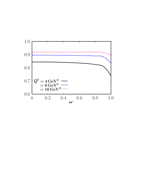
Figure 5: The ratio of the transition form factors evaluated from (49) and from the collinear result (71) versus $\omega$ for a set of $\overline{Q}^{2}$ values. The form factors are evaluated from the wave function (31) and the associated distribution amplitude (33), respectively.

Here, in this subsection, it will be commented on the $\gamma^{*}-f_{0}$ transition form factor. As is the case for $\omega=1$, the Sudakov factor plays a minor role. In order to estimate the importance of the power corrections taken into account in the modified perturbative approach the ratio of the form factors evaluated from (49) (transformed to the impact parameter plane and with the Sudakov factor included) and from the collinear approximation

$$F_{T}^{\rm coll}(\overline{Q}^{2},\omega)\,=\,-\frac{e_{s}^{2}}{\overline{Q}^{2}}\bar{f}_{0}M_{0}\frac{\omega^{2}+\frac{1}{2}\frac{M_{0}^{2}}{\overline{Q}^{2}}}{1+\frac{1}{2}\frac{M_{0}^{2}}{\overline{Q}^{2}}}\int d\xi\frac{\xi\Phi_{0}(\xi)}{1-\xi^{2}\omega^{2}}$$ (71)

is displayed in Fig. 5. As expected the power corrections become smaller with increasing $\overline{Q}^{2}$ and their importance decreases if $\omega$ deviates from 1. The same observation has been made in [35] in case of the $\gamma^{*}-\pi$ transition form factor. As noticed in [35] the reason for this effect is the term $1-\xi^{2}\omega^{2}$ in the hard scattering kernel which controls to which extent the form factor is sensitive to contributions from the end-point regions $\xi\to\pm 1$ where soft effects can be important.

Since the power corrections are small at small $\omega$, it is of interest to look at the transition form factor (71) in this region. Using the Gegenbauer expansion of the distribution amplitude the integral can be carried out term by term. The full result is a power series in $\omega^{2}$ leaving aside the $\omega$-dependence of the prefactor. The first terms of this series read

$$F_{T}^{\rm coll}(\overline{Q}^{2},\omega) = -\frac{2}{5}N_{c}e_{s}^{2}\frac{\bar{f}_{0}M_{0}}{\overline{Q}^{2}}\frac{\omega^{2}+\frac{1}{2}\frac{M_{0}^{2}}{\overline{Q}^{2}}}{1+\frac{1}{2}\frac{M_{0}^{2}}{\overline{Q}^{2}}}\Big{[}B_{1}+\omega^{2}\frac{3}{7}\big{(}B_{1}+\frac{20}{27}B_{3}\big{)}$$ (72)

$$+ \omega^{4}\frac{5}{21}\big{(}B_{1}+\frac{40}{33}B_{3}+\frac{56}{143}B_{5}\big{)}+\ldots\Big{]}\,.$$

As one notices the $m$-th Gegenbauer coefficient comes with the power $\omega^{m-1}$ first. For $\overline{Q}^{2}$ larger than $4\,~{}{\rm GeV}^{2}$ the difference between the modified perturbative approach and the collinear result is smaller than $10\%$. Hence, the result in the modified perturbative approach evaluated from the wave function (26), is not far from the collinear result (72). Thus, as is the case for the $\gamma^{*}-\pi$ transition form factor [35], a measurement of the $\gamma^{*}-f_{0}$ transition form factors for a range of small $\omega$ would therefore provide valuable constraints on the $f_{0}$ distribution amplitude.

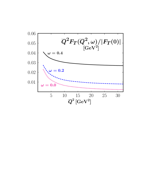
Figure 6: The $\gamma^{*}-f_{0}$ transition form factor, scaled by $|F_{T}(0)|/\overline{Q}^{2}$, evaluated from the wave function (31) (with $B_{1}=-0.57$) within the modified perturbative approach versus $\overline{Q}^{2}$ for a set of $\omega$ values.

In Fig. 6 the $\gamma^{*}-f_{0}$ transition form factor, evaluated from the wave function (31) within the modified perturbative approach, is shown for several small values of $\omega$. It is clearly seen that the form factor drops with $\overline{Q}^{2}$ increasingly stronger than $1/\overline{Q}^{2}$ with decreasing $\omega$. At $\omega=0$ it decreases as $1/\overline{Q}^{4}$ (aside from evolution logarithms).

5 Summary

In this article the spin wave function of the $f_{0}(980)$ meson is constructed under the assumption that the meson is dominantly a strange-antistrange quark state. The collinear limit of the spin wave function is also discussed and the connection to the twist-2 and twist-3 distribution amplitudes is made. The spin wave function is applied in a calculation of the $\gamma^{*}-f_{0}$ transition form factors. In the real-photon limit the results for the transverse form factor are compared to the large-$Q^{2}$ data measured by the BELLE collaboration recently. It turns out that, for the $Q^{2}$ range explored by BELLE, the collinear approximation does not suffice, power corrections to it, modeled as quark transverse moment effects, seem to be needed. The parameters required in this calculation in order to achieve agreement with BELLE form factor data, the transverse-size parameter, $a_{0}$, the decay constant, $\bar{f}_{0}$, and the lowest (effective) Gegenbauer coefficient, $B_{1}$, have plausible values. However, Cheng et al [10] in their analysis of charmless $B$-meson decays, adopt a much larger value for $\bar{f}_{0}$ than (35). It remains to be seen whether the $B$-meson decays can be reconciled with the decay constant (35). The implications of $\sigma-f_{0}$ mixing for the transition form factors are also briefly discussed. A mixing angle of about $150^{\circ}$ seems to be favored. The paper is completed by presenting results on the $\gamma^{*}-f_{0}$ form factors and on their collinear limits. It turns out that, in many aspects, the photon - $f_{0}$ form factors have properties similar to the form factors for the transition from a photon to the $\pi^{0}$ or other pseudoscalar mesons. However, the limits for $Q_{1}^{2}\to\infty$ are different. Whereas for the pseudoscalar mesons the limits of the scaled form factors are finite (e.g. $Q_{1}^{2}F_{\gamma\pi^{0}}\to\sqrt{2}f_{\pi}$) the $\gamma-f_{0}$ form factor $F_{T}$ tends to zero $\sim f_{0}(\mu_{0})B_{1}(\mu_{0})(\alpha_{s}(\mu_{0})/\alpha_{s}(Q_{1}^{2}))^{-4/25}$. The $\gamma^{*}-f_{0}$ transition form factors also play a role in the calculation of the hadronic light-by-light contribution to the muon anomalous magnetic moment [40] - [43]. In particular, the results presented in this article clarify the asymptotic behavior of the $\gamma^{*}-f_{0}$ form factors.

Acknowledgements: Thanks to Volodya Braun and Andreas Schäfer for suggesting this study and for discussions. The work is supported in part by the BMBF, contract number 05P12WRFTE.

References

- [1] M. Masuda et al. [Belle Collaboration], Phys. Rev. D 93, no. 3, 032003 (2016).
- [2] G. A. Schuler, F. A. Berends and R. van Gulik, Nucl. Phys. B 523, 423 (1998).
- [3] G. T. Bodwin, E. Braaten and G. P. Lepage, Phys. Rev. D 51, 1125 (1995) [Phys. Rev. D 55, 5853 (1997)].
- [4] V. Pascalutsa, V. Pauk and M. Vanderhaeghen, Phys. Rev. D 85, 116001 (2012).
- [5] V. M. Braun, N. Kivel, M. Strohmaier and A. A. Vladimirov, JHEP 1606, 039 (2016).
- [6] N. N. Achasov, A. V. Kiselev and G. N. Shestakov, JETP Lett. 102, no. 9, 571 (2015) [Pisma Zh. Eksp. Teor. Fiz. 102, no. 9, 655 (2015)].
- [7] M. Diehl, T. Gousset, B. Pire and O. Teryaev, Phys. Rev. Lett. 81, 1782 (1998).
- [8] K. A. Olive et al. [Particle Data Group Collaboration], Chin. Phys. C 38, 090001 (2014); update 2015.
- [9] W. Ochs, J. Phys. G 40, 043001 (2013).
- [10] H. Y. Cheng, C. K. Chua and K. C. Yang, Phys. Rev. D 73, 014017 (2006).
- [11] S. Stone and L. Zhang, Phys. Rev. Lett. 111, no. 6, 062001 (2013).
- [12] Z. Q. Zhang, S. Y. Wang and X. K. Ma, Phys. Rev. D 93, no. 5, 054034 (2016).
- [13] R. L. Jaffe and F. Wilczek, Phys. Rev. Lett. 91, 232003 (2003).
- [14] L. Maiani, F. Piccinini, A. D. Polosa and V. Riquer, Phys. Rev. Lett. 93, 212002 (2004).
- [15] G. ’t Hooft, G. Isidori, L. Maiani, A. D. Polosa and V. Riquer, Phys. Lett. B 662, 424 (2008).
- [16] V. Baru, J. Haidenbauer, C. Hanhart, Y. Kalashnikova and A. E. Kudryavtsev, Phys. Lett. B 586, 53 (2004).
- [17] G. P. Lepage and S. J. Brodsky, Phys. Lett. B 87, 359 (1979).
- [18] S. J. Brodsky, T. Huang and G. P. Lepage, Conf. Proc. C 810816, 143 (1981).
- [19] P. A. M. Dirac, Rev. Mod. Phys. 21, 392 (1949).
- [20] H. Leutwyler and J. Stern, Annals Phys. 112, 94 (1978).
- [21] J. Bolz, P. Kroll and J. G. Körner, Z. Phys. A 350, 145 (1994).
- [22] Z. Dziembowski, Phys. Rev. D 37, 768 (1988).
- [23] F. Hussain, J. G. Körner and G. Thompson, Annals Phys. 206, 334 (1991).
- [24] X. d. Ji, J. P. Ma and F. Yuan, Eur. Phys. J. C 33, 75 (2004).
- [25] M. Beneke, G. Buchalla, M. Neubert and C. T. Sachrajda, Nucl. Phys. B 591, 313 (2000).
- [26] J. Bolz, P. Kroll and G. A. Schuler, Eur. Phys. J. C 2, 705 (1998).
- [27] V. L. Chernyak and A. R. Zhitnitsky, Phys. Rept. 112, 173 (1984).
- [28] C. D. Lu, Y. M. Wang and H. Zou, Phys. Rev. D 75, 056001 (2007).
- [29] M. Beneke and T. Feldmann, Nucl. Phys. B 592, 3 (2001).
- [30] H. W. Huang, R. Jakob, P. Kroll and K. Passek-Kumericki, Eur. Phys. J. C 33, 91 (2004).
- [31] P. Kroll, Eur. Phys. J. C 71, 1623 (2011).
- [32] S. V. Goloskokov and P. Kroll, Eur. Phys. J. C 65, 137 (2010).
- [33] F. De Fazio and M. R. Pennington, Phys. Lett. B 521, 15 (2001).
- [34] I. Bediaga, F. S. Navarra and M. Nielsen, Phys. Lett. B 579, 59 (2004).
- [35] M. Diehl, P. Kroll and C. Vogt, Eur. Phys. J. C 22, 439 (2001).
- [36] H. n. Li and G. F. Sterman, Nucl. Phys. B 381, 129 (1992).
- [37] T. Feldmann, P. Kroll and B. Stech, Phys. Rev. D 58, 114006 (1998).
- [38] P. Kroll and K. Passek-Kumericki, Phys. Rev. D 67, 054017 (2003).
- [39] H. Y. Cheng and K. C. Yang, Phys. Rev. D 71, 054020 (2005).
- [40] V. Pauk and M. Vanderhaeghen, Eur. Phys. J. C 74, no. 8, 3008 (2014).
- [41] G. Colangelo, M. Hoferichter, M. Procura and P. Stoffer, JHEP 1409, 091 (2014).
- [42] A. E. Dorokhov, A. E. Radzhabov and A. S. Zhevlakov, Eur. Phys. J. C 75, no. 9, 417 (2015).
- [43] F. Jegerlehner and A. Nyffeler, Phys. Rept. 477, 1 (2009)