Energy-Aware Wireless Relay Selection in Load-Coupled OFDMA Cellular Networks

Abstract

We investigate transmission energy minimization via optimizing wireless relay selection in orthogonal-frequency-division multiple access (OFDMA) networks. We take into account the impact of the load of cells on transmission energy. We prove the $\mathcal{NP}$-hardness of the energy-aware wireless relay selection problem. To tackle the computational complexity, a partial optimality condition is derived for providing insights in respect of designing an effective and efficient algorithm. Numerical results show that the resulting algorithm achieves high energy performance.

I Introduction

Relay techniques provide coverage extension, alleviate fading effects in wireless channels, and lead to more rapid network roll-out to improve the overall system energy efficiency [1, 2, 3]. In meeting the fast growing demand of mobile communication and the increase of user density, wireless relaying is viewed as a promising technique for the upcoming 5G [4]. It is shown that wireless backhaul technologies have competitive advantages over the fiber-based solution [5]. In 5G, outdoor relays are likely to be densely deployed in urban areas, which may cause the cost of installing fiber-based relay nodes to reach an unacceptable level. For the indoor scenarios, wireless backhauling may provide better flexibility and cost-efficiency, compared to a fiber-based solution [6]. In addition, though fiber-based backhauling has advantage in capacity, reliability, and robustness for transmission, there are cases in which wired backhauling is impossible (e.g. short-term links for emergency/disaster relief), hence making the wireless solution to be the only option for such scenarios [5].

There are two types of relaying modes in terms of wireless backhauling [6, 7]. One is called “out-band” mode, in which the backhaul and access links operate on different carriers. The other is “in-band” mode, meaning that there is no explicit splitting in frequency resource between backhaul links and access links [6, 7]. Compared to the former, the latter does not require a pre-defined separation in the frequency domain. Moreover, if relays are required to operate on a single carrier, then there is no possibility to make separation for implementing out-band relay mode, and thus in-band relay would be the only option in this case [7].

Recently, studies [8, 9] investigated energy minimization in orthogonal-frequency-division multiple access (OFDMA) networks, under an interference model proposed in [10]. This model characterizes the coupling relationship among the load of cells, which is defined to be the proportion of consumed time-frequency resource in each cell. The model is therefore named as a “load-coupling” model [10]. However, understanding and analyzing load coupling for relays with wireless backhauling is not straightforward. In this paper, we provide significant extensions of the model to wireless relay scenarios, following the LTE-advanced standard of wireless relays in[6]. We formulate the energy-aware relay selection problem, named MinE, and prove its computational hardness. Moreover, we derive an optimality condition, based on which a relay selection algorithm is proposed for solving MinE. Numerical results show significant improvement on network energy consumption, compared to the standard strategy of strongest-cell association.

II System Model

II-A Network Model

We consider a heterogeneous cellular network (HetNet) with macro cells (MCs), user equipments (UEs), and relay cells (RCs). Denote by $\mathcal{B}=\{1,2,\ldots,n_{\mathcal{B}}\}$ the set of MCs, $\mathcal{T}=\{1,2,\ldots,n_{\mathcal{T}}\}$ the set of UEs, and $\mathcal{R}=\{n_{\mathcal{T}}+1,n_{\mathcal{T}}+2,\ldots,n_{\mathcal{T}}+n_{\mathcal{R}}\}$ the set of RCs. We focus on downlink transmission in this paper. For any UE $j\in\mathcal{T}$, the set of $j$’s candidate serving cells is denoted by $\mathcal{C}_{j}$. For any RC $k\in\mathcal{R}$, denote by $\mathcal{C}_{k}$ the set of $k$’s candidate MCs for establishing the backhaul link. The relay selection aims at 1) choosing a serving cell out of $\mathcal{C}_{j}$ for all $j\in\mathcal{T}$, and 2) finding for each RC $k\in\mathcal{R}$ an MC out of $\mathcal{C}_{k}$ to establish the backhaul link, so as to minimize the network transmission energy.

We assume in-band wireless relay transmission [11], which implies no explicit splitting of available time-frequency resource between the backhaul links and the access links. To avoid the loop interference [7], the backhaul and access links should operate on orthogonal resources, meaning that, within the area of each MC, the time-frequency resource units (RUs) utilized by the two types of links do not overlap. Thus some of the links preserve orthogonality with each other. We refer to Figure 1 for an illustration.

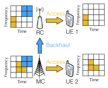
Figure 1: Illustration of the HetNet model. In this example, there are one MC, one RC, and two UEs. UE 1 and UE 2 are served by the RC and MC, respectively. The RC is doing a wireless backhauling with the MC. The used resource for access links and backhaul links is marked by yellow and blue colors, respectively. In time and frequency, the resource allocated to backhauling has orthogonality to the resource used by the access links.

In the remaining parts of this paper, we use the term “orthogonal links” to refer to those links using orthogonal time-frequency resource for transmission. Such links are said to be orthogonal to each other. Below, we discuss the characterization of orthogonality. For the sake of presentation, consider given association of UE access and RC backhauling, and denote by $\mathcal{R}_{i}$ the set of RCs with a wireless backhaul connected to MC $i$ for each $i\in\mathcal{B}$. The set of UEs served by any cell (MC or RC) $i$ is represented by $\mathcal{T}_{i}$. Denote by tuple $\langle i,j\rangle$ any (backhaul or access) link from $i$ to $j$. For any access link $\langle i,j\rangle$ with $i\in\mathcal{B}$ and $j\in\mathcal{T}_{i}$, denote by $\mathcal{L}_{ij}=\{\langle i,v\rangle:v\in\mathcal{R}_{i}\cup\mathcal{T}_{i}\}$ the set of links that preserve orthogonality to link $\langle i,j\rangle$. For $k\in\mathcal{R}$, suppose that it is connected with some MC $i$ with a backhaul link. We define $\mathcal{L}_{kj}=\{\langle k,v\rangle:v\in\mathcal{T}_{k}\}\cup\{\langle i,k\rangle\}$ to be the set of links having the intra-cell orthogonality to the access link $\langle k,j\rangle$ with $j\in\mathcal{T}_{k}$. And for the backhaul link $\langle i,k\rangle$, we define $\mathcal{L}_{ik}=\{\langle i,v\rangle:v\in\mathcal{R}_{i}\cup\mathcal{T}_{i}\}\cup\{\langle k,v\rangle:v\in\mathcal{T}_{k}\}$ the set $\mathcal{L}_{ik}$. We denote by $\mathcal{L}$ the set of all backhaul and access links in the network.

II-B Load-Coupling Model

Let $r_{ij}$ be the bit rate demand on the link $\langle i,j\rangle$. Denote by $\gamma_{ij}$ the signal-to-interference-and-noise ratio (SINR) from $i$ to $j$. Without loss of generality, we use an (RU) to refer to the minimum unit for resource allocation. The bandwidth per RU is denoted by $B$. In the denominator in (1), $B\log_{2}(1+\gamma_{ij})$ computes the achievable bit rate per RU. We assume that there are $M$ RUs in total, such that $MB\log_{2}(1+\gamma_{ij})$ is the total achievable bit rate for UE $j$. In (1), $x_{ij}$ is then defined to be the proportion of RUs used by the transmission link $\langle i,j\rangle$, among all RUs in cell $i$. The sum of the proportion of allocated RUs in any cell $i$, i.e., $\sum_{j\in\mathcal{T}_{i}}x_{ij}$, is defined to be the load of cell $i$, which is bounded by the full load, i.e. $\sum_{j\in\mathcal{T}_{i}}x_{ij}\leq 1\leavevmode\nobreak\ i\in\mathcal{B}\cup\mathcal{R}$.

$$x_{ij}=\frac{r_{ij}}{MB\log_{2}(1+\gamma_{ij})}$$ (1)

The SINR on any RU allocated to $\langle i,j\rangle$ is given by (2). In the nominator, $p_{ij}$ is the transmission power of an RU of link $\langle i,j\rangle$ in cell $i$. The value of $g_{ij}$ is the power gain from $i$ to $j$. In the denominator of (2), recall that $x_{vu}$ represents the proportion of occupied RU by $\langle v,u\rangle$ in cell $v$. The value of $x_{vu}$ is then interpreted as the likelihood that $\langle i,j\rangle$ receives interference from $\langle v,u\rangle$ on the RU. Note that $\langle v,u\rangle\in\mathcal{L}\backslash\mathcal{L}_{ij}$, which is the set of all links that are not required to be orthogonal to $\langle i,j\rangle$.

$$\gamma_{ij}=\frac{p_{ij}g_{ij}}{\sum_{\langle v,u\rangle\in\mathcal{L}\backslash\mathcal{L}_{ij}}p_{vu}g_{vj}x_{vu}+\sigma^{2}}$$ (2)

By (1) and (2), one can observe that a change on $x_{uv}$ for any link $\langle u,v\rangle$ may cause a variation after the SINR of some link $\langle i,j\rangle$, thus leading to a new value of $x_{ij}$, i.e., the required resource consumption for link $\langle i,j\rangle$. Thus, the levels of resource consumption are inherently coupled. This relationship, as characterized by (1) and (2), is called load-coupling.

II-C Computation of Transmission Energy

Recall that $x_{ij}$ represents the proportion of consumed RU of link $\langle i,j\rangle$. Hence, the number of RUs that are used for transmission by $\langle i,j\rangle$ is $Mx_{ij}$. On each RU, the transmit power is $p_{ij}$. Then the energy consumption on link $\langle i,j\rangle$ is $Mp_{ij}x_{ij}$. We now focus on how to compute $x_{ij}$ in the load-coupling model in (1) and (2). Let $n=n_{\mathcal{T}}+n_{\mathcal{R}}$. The proportions of RU consumption for all potential links in the network are represented by the vector $\bm{x}=[\leavevmode\nobreak\ {[x_{11},\dots,x_{|\mathcal{C}_{1}|1}]},\dots,{[x_{1n},\dots,x_{|\mathcal{C}_{n}|n}]}\leavevmode\nobreak\ ]$.

By plugging (2) in (1), we get the function of the proportion of consumed RUs by $\langle i,j\rangle$ in (3) below. For vector $\bm{x}$ satisfying the cell-load coupling relation in the system model $x_{ij}=F_{ij}(\bm{x})$ holds for all $\langle i,j\rangle\in\mathcal{L}$.

$$F_{ij}(\bm{x})=\frac{r_{ij}}{MB\log_{2}(1+\frac{p_{ij}g_{ij}}{\sum\limits_{\langle v,u\rangle\in\mathcal{L}\backslash\mathcal{L}_{ij}}p_{uv}g_{uj}x_{uv}+\sigma^{2}})}$$ (3)

It can be verified by observing the concavity of function $F_{ij}(\bm{x})$ that $F_{ij}$ is a standard interference function (SIF) in respect of $\bm{x}$ [8, 12]. An SIF has the following property: starting from an arbitrary positive $\bm{x}^{(0)}$, if the fixed point of function $F_{ij}$ exists, then it is unique, can be iteratively computed by $x^{(k)}_{ij}=F_{ij}(\bm{x}^{(k-1)})$ $(k\geq 1)$.

III Problem Formulation

For any UE $j\in\mathcal{T}$, we use a variable $a_{j}$ to indicate the UE’s serving cell, i.e. $a_{j}=i$ if UE $j$ is currently served by cell $i$. Similarly, for any RC $k\in\mathcal{R}$, we use $a_{k}=i$ to indicate that RC $k$ is connected to MC $i$ with a wireless backhaul. For any $j$, $a_{j}\in\mathcal{C}_{j}$ for all $j\in\mathcal{T}\cup\mathcal{R}$. The vector $\bm{a}$ then denotes the association among MCs, RCs and UEs.

$$[\textit{MinE}]\quad \min\limits_{\bm{x},\bm{a},\bm{r}}\quad M\sum_{j=1}^{n}p_{a_{j}j}x_{a_{j}j}$$ (4a)

$$s.t.\quad \bm{x}=\bm{F}(\bm{x},\bm{a},\bm{r})$$ (4b)

$$r_{a_{j}j}=d_{j}\quad j\in\mathcal{T}$$ (4c)

$$r_{a_{k}k}=\sum_{j\in\mathcal{T}_{k}}d_{j}\quad k\in\mathcal{R}$$ (4d)

$$\sum_{k\in\mathcal{R}:a_{k}=i}x_{ik}+\sum_{j\in\mathcal{T}:a_{j}=i}x_{ij}\leq 1\quad i\in\mathcal{B}$$ (4e)

$$x_{a_{k}k}+\sum_{j\in\mathcal{T}:a_{j}=k}x_{kj}\leq 1\quad k\in\mathcal{R}$$ (4f)

$$a_{j}\in\mathcal{C}_{j}\quad j\in\mathcal{T}\cup\mathcal{R}$$ (4g)

The energy-aware relay selection problem, a.k.a. MinE, is formulated in (4). The objective of minimizing the energy on all links is given in (4a). Constraint (4b) ensures that $\bm{x}$ satisfies the coupling relationship in the system model. Constraint (4c) guarantees that the bit rate demand of any UE $j\in\mathcal{T}$ is satisfied. Constraint (4d) ensures sufficient bit rate on each backhaul link. Constraint (4e) and (4f) are imposed to limit the proportion of consumed RUs in each cell to be no more than 1, corresponding to the full load constraint for MCs and RCs, respectively. Constraint (4g) is imposed such that the selected cell for a backhaul/access link is within the candidate set.

IV Complexity Analysis

Theorem 1.

MinE is $\mathcal{NP}$-hard.

Proof.

We reduce the Maximum Independent Set (MIS) problem to MinE. We construct a specific HetNet scenario. For each UE, there is one potential MC and one potential RC as candidate serving cells. Correspondingly, for any undirected graph instance $\mathcal{G}$ with $N$ nodes ($N\geq 2$) in the MIS problem, we define $N$ UEs. Thus, for any node in $\mathcal{G}$, we have one UE, one MC and one RC. We use $1,2,\ldots,N$ to index the nodes in graph $\mathcal{G}$. We use the term “neighboring” to refer to the relationship of any two entities that are associated respectively to two neighboring nodes in $\mathcal{G}$.

For any node $i$ in $\mathcal{G}$, we set the gain from MC $i$ to UE $i$ to $1.0$, the gain from RC $i$ to UE $i$ to $6.0$, and the gain from MC $i$ to RC $i$ to $3.0$, respectively. For any two neighbouring nodes $i$ and $k$ (meaning that there is an edge between node $i$ and node $k$) in graph $\mathcal{G}$, we set the gain from RC $i$ to UE $k$ to a small positive value $\epsilon$. The gain values other than the above three cases are set to be negligible, treated as zero. The noise $\sigma^{2}$ is set to $1.0$. The values of gain and noise can be scaled without affecting the validity of the proof. The transmit powers of MCs and RCs are set to $1.0$ and $0.5$, respectively.The bit rate demand for any UE is set to $1.0$.

Due to space limit, we give a sketch of the line of arguments. For any UE $i$, if we have it served by RC $i$, then all the resource in RC $i$ is in use. If any RC $k$ neighboring to UE $i$ is activated, then UE $i$ would receive the interference from RC $k$, leading to that UE $i$’s demand cannot be satisfied anymore by the access link from RC $i$ to UE $i$. Hence in a feasible solution, any pair of two neighboring UEs cannot be simultaneously served by their corresponding RCs. In addition, one can verify that it is always better to serve any UE $i$ with RC $i$ rather than MC $i$ for energy saving. Thus we finish the reduction by concluding that, to solve this constructed problem instance is to maximize the number of activated RCs, subject to that at most one RC of any pair of neighboring RCs can be in use. Hence the conclusion. ∎

V Energy Minimization via Optimality Condition

This section aims to seek for an effective strategy to deal with the combinatorial nature of MinE. A partial optimality condition is derived below, based on which we propose the relay selection algorithm.

V-A Optimality Condition

We introduce some notations for deriving the optimality condition. Denote by $\hat{\bm{a}}$ and $\check{\bm{a}}$ any two associations, such that $\exists j$ $\hat{a}_{j}\neq\check{a}_{j}$. Denote $\mathpzc{l}=\{j:\hat{a}_{j}\neq\check{a}_{j},\leavevmode\nobreak\ j\in\mathcal{T}\cup\mathcal{R}\}$. Denote by $\hat{\bm{x}}$ and $\check{\bm{x}}$ the fixed points of the function $\bm{F}$ under $\hat{\bm{a}}$ and $\check{\bm{a}}$, respectively. Denote by $\hat{e}$ the total transmission energy with association $\hat{\bm{a}}$, i.e. $\hat{e}=\sum_{j=1}^{n}p_{\hat{a}_{j}j}\hat{x}_{\hat{a}_{j}j}$, and by $\check{e}$ the total transmission energy with association $\check{\bm{a}}$, i.e. $\check{e}=\sum_{j=1}^{n}p_{\check{a}_{j}j}\check{x}_{\check{a}_{j}j}$.

Definition 1.

We define the following function for any $i\in\mathcal{C}_{j}$, and any $j\in\mathcal{T}\cup\mathcal{R}$, where $\mathpzc{t}$ is a non-empty subset of $\mathcal{T}\cup\mathcal{R}$.

$$G_{ij}(\bm{x},\bm{a},\mathpzc{t})=\left\{\begin{array}[]{ll}F_{ij}(\bm{x},\bm{a})&j\in\mathpzc{t}\\ x_{ij}&\textnormal{otherwise}\end{array}\right.$$ (5)

Theorem 2.

(Optimality Condition) $\hat{e}<\check{e}$ if and only if for some set $\mathpzc{t}$ $(\mathpzc{l}\subseteq\mathpzc{t}\subseteq\mathcal{T}\cup\mathcal{R})$ such that:

1. $\sum_{j\in\mathpzc{t}}p_{\hat{a}_{j}j}x^{\mathpzc{t}}_{\hat{a}_{j}j}<\sum_{j\in\mathpzc{t}}p_{\check{a}_{j}j}\check{x}_{\check{a}_{j}j}$ where any $x^{\mathpzc{t}}_{\hat{a}_{j}j}$ with $j\in\mathcal{T}\cup\mathcal{R}$ is an element of $\bm{x}^{\mathpzc{t}}$, and $\bm{x}^{\mathpzc{t}}$ is the fixed point of $\bm{G}(\bm{x},\hat{\bm{a}},\mathpzc{t})$, with $\check{\bm{x}}$ being the starting point.

2. $F_{\hat{a}_{j}j}(\bm{x}^{\mathpzc{t}},\hat{\bm{a}})\leq\check{x}_{\check{a}_{j}j}$ for any $j\notin\mathpzc{t}$.

Proof.

The necessity can be proved straightforwardly by letting $\mathpzc{t}=\mathcal{T}\cup\mathcal{R}$. For the sufficiency, the basic idea is to prove $\hat{\bm{x}}\leq\bm{x}^{\mathpzc{t}}$ by using Condition 2), and then combine it with Condition 1) to compute respectively $\hat{e}$ and $\check{e}$. Suppose there exists some set $\mathpzc{t}$ ($\mathpzc{l}\subseteq\mathpzc{t}\subseteq\mathcal{T}\cup\mathcal{R}$) satisfying 1) and 2). We consider the fixed-point iterations $\hat{\bm{x}}^{(k)}=\bm{F}(\hat{\bm{x}}^{(k-1)},\hat{\bm{a}})$ $(k\geq 0)$. Let $\hat{\bm{x}}^{(0)}=\bm{x}^{\mathpzc{t}}$. For $j\in\mathpzc{t}$, since $x^{\mathpzc{t}}_{\hat{a}_{j}j}=G_{\hat{a}_{j}j}(\bm{x}^{\mathpzc{t}},\hat{\bm{a}},\mathpzc{t})=F_{\hat{a}_{j}j}(\bm{x}^{\mathpzc{t}},\hat{\bm{a}})$, combined with the construction that $\hat{\bm{x}}^{(0)}=\bm{x}^{\mathpzc{t}}$, we have $\hat{x}_{\hat{a}_{j}j}^{(1)}=F_{\hat{a}_{j}j}(\hat{\bm{x}}^{(0)},\hat{\bm{a}})=G_{\hat{a}_{j}j}(\hat{\bm{x}}^{(0)},\hat{\bm{a}},\mathpzc{t})=G_{\hat{a}_{j}j}(\bm{x}^{\mathpzc{t}},\hat{\bm{a}},\mathpzc{t})=x^{\mathpzc{t}}_{\hat{a}_{j}j}=\hat{x}^{(0)}_{\hat{a}_{j}j}$. For $j\notin\mathpzc{t}$, we have $\hat{x}_{\hat{a}_{j}j}^{(1)}=F_{\hat{a}_{j}j}(\hat{\bm{x}}^{(0)},\hat{\bm{a}})$. By the construction that $\hat{\bm{x}}^{(0)}=\bm{x}^{\mathpzc{t}}$ and condition 2), $\hat{x}_{\hat{a}_{j}j}^{(1)}=F_{\hat{a}_{j}j}(\hat{\bm{x}}^{(0)},\hat{\bm{a}})=F_{\hat{a}_{j}j}(\bm{x}^{\mathpzc{t}},\hat{\bm{a}})\leq x_{\hat{a}_{j}j}^{\mathpzc{t}}=\hat{x}_{\hat{a}_{j}j}^{(0)}$ holds. Therefore, we have

$$\hat{\bm{x}}^{(1)}\leq\hat{\bm{x}}^{(0)}=\bm{x}^{\mathpzc{t}}.$$ (6)

We first consider $\hat{e}$. By the monotonicity of $\bm{F}(\bm{x},\hat{\bm{a}})$ in $\bm{x}$, we have the following property. For any $k\geq 0$, if $\bm{x}^{(k)}\leq\bm{x}^{(k-1)}$, then $\bm{F}(\bm{x}^{(k)},\hat{\bm{a}})\leq\bm{F}(\bm{x}^{(k-1)},\hat{\bm{a}})$ holds, which would directly lead to $\bm{x}^{(k+1)}\leq\bm{x}^{(k)}$. According to the discussion above, we have $\bm{x}^{(k+1)}\leq\bm{x}^{(k)}$ for $k=0$. We therefore conclude by mathematical induction that $\hat{\bm{x}}\leq\cdots\leq\hat{\bm{x}}^{(1)}\leq\hat{\bm{x}}^{(0)}=\bm{x}^{\mathpzc{t}}$. Thus, we have

$$\hat{e}\leq\sum_{j=1}^{n}p_{\hat{a}_{j}j}x^{\mathpzc{t}}_{\hat{a}_{j}j}$$ (7)

We then consider $\check{e}$. For any $j\notin\mathpzc{t}$, we have $x_{\hat{a}_{j}j}^{\mathpzc{t}}=G_{\hat{a}_{j}j}(\bm{x}^{\mathpzc{t}},\hat{\bm{a}},\mathpzc{t})$. Since $\mathpzc{l}\subseteq\mathpzc{t}$, we conclude $j\notin\mathpzc{l}$ for any $j\notin\mathpzc{t}$. Therefore, according to the definition of $\mathpzc{l}$, we have $\hat{a}_{j}=\check{a}_{j}$ for $j\notin\mathpzc{t}$. Note that in condition 1), $\check{\bm{x}}$ is the starting point for the fixed-point iterations of the function $\bm{G}(\bm{x},\check{\bm{a}},\mathpzc{t})$. According to the definition of the function $G_{ij}$ in (5), for any $j\notin\mathpzc{t}$, we have $x^{\mathpzc{t}}_{\hat{a}_{j}j}=\check{x}_{\hat{a}_{j}j}=\check{x}_{\check{a}_{j}j}$. Thus we conclude $\sum_{j\notin\mathpzc{t}}p_{\hat{a}_{j}j}x^{\mathpzc{t}}_{\hat{a}_{j}j}=\sum_{j\notin\mathpzc{t}}p_{\check{a}_{j}j}x_{\check{a}_{j}j}$. For any $j\in\mathpzc{t}$, condition 1) shows that $\sum_{j\in\mathpzc{t}}p_{\hat{a}_{j}j}x^{\mathpzc{t}}_{\hat{a}_{j}j}<\sum_{j\in\mathpzc{t}}p_{\check{a}_{j}j}\check{x}_{\check{a}_{j}j}$. Therefore, we obtain

$$\check{e}>\sum_{j=1}^{n}p_{\hat{a}_{j}j}x^{\mathpzc{t}}_{\hat{a}_{j}j}$$ (8)

Hence the conclusion $\hat{e}<\check{e}$. ∎

Given any two associations $\hat{\bm{a}}$ and $\check{\bm{a}}$, Theorem 2 serves as a sufficient and necessary condition for checking whether $\hat{\bm{a}}$ leads to a better energy performance than $\check{\bm{a}}$. When $\mathpzc{t}\subset\mathcal{T}\cup\mathcal{R}$, it is called asynchronous fixed-point iterations [12], which is rather faster if $|\mathpzc{t}|\ll|\mathcal{T}\cup\mathcal{R}|$ and can be implemented in a distributed manner.

V-B Algorithm Design

We use the function $A_{j}(\bm{x})=\operatorname{\arg\min}\limits_{i\in\mathcal{C}_{j}}p_{ij}x_{ij}$ to assign each $j\in\mathcal{T}\cup\mathcal{R}$ to the cell with lowest energy for transmitting to $j$. Algorithm 1 below takes an initial association $\check{\bm{a}}$ as the input, and outputs the optimized association $\hat{\bm{a}}$. The pre-defined parameter $\eta$ indicates the maximum number of loop rounds. The vectors $\bm{a}$ and $\bm{x}$ are iteratively updated by functions $\bm{A}$ and $\bm{F}$, respectively. Once $\bm{a}^{(k)}=\bm{a}^{(k-1)}$ holds for any round $k$, meaning that there is no update on vector $\bm{a}^{(k)}$, the algorithm terminates and returns the optimized association $\hat{\bm{a}}$. In each round, the set $\mathpzc{l}^{(k)}$ records the positions of all the different elements between $\bm{a}^{(k)}$ and $\check{\bm{a}}$. In Lines 1 and 1, the asynchronous fixed-point iterations are applied with respect to set $\mathpzc{t}$, with $\mathpzc{t}\supseteq\mathpzc{l}^{(k)}$. Lines 1 and 1 use the optimality condition to check if the new association $\bm{a}^{(k)}$ would improve the transmission energy, with numerical tolerances $\epsilon_{1}$ and $\epsilon_{2}$.

1 $\bm{a}^{(0)}\leftarrow\check{\bm{a}}$, $\hat{\bm{a}}\leftarrow\check{\bm{a}}$;

2 $\bm{x}^{(0)}\leftarrow$ fixed point of $\bm{F}(\bm{x},\bm{a}^{(0)})$;

3 for $k\leftarrow 1\leavevmode\nobreak\ \textnormal{{to}}\leavevmode\nobreak\ \eta$ do

4        $\bm{a}^{(k)}\leftarrow\bm{A}(\bm{x}^{(k-1)})$;

5        if $\bm{a}^{(k)}=\bm{a}^{(k-1)}$ then

6              break;

7       $\bm{x}^{(k)}\leftarrow\bm{F}(\bm{x}^{(k-1)},\bm{a}^{(k)})$;

8        $\mathpzc{l}^{(k)}\leftarrow\{j:a^{(k)}_{j}\neq\check{a}_{j},\leavevmode\nobreak\ j\in\mathcal{T}\cup\mathcal{R}\}$;

9        choose a set $\mathpzc{t}$ such that $\mathpzc{l}^{(k)}\subseteq\mathpzc{t}$;

10        $\bm{x}^{\mathpzc{t}}\leftarrow$ fixed point of $\bm{G}(\bm{x},\hat{\bm{a}},\mathpzc{t})$, starting from $\bm{x}^{(k)}$;

11        if $\sum_{j\in\mathpzc{t}}p_{a_{j}^{(k)}j}x^{\mathpzc{t}}_{a_{j}^{(k)}j}<\sum_{j\in\mathpzc{t}}p_{\check{a}_{j}j}\check{x}_{\check{a}_{j}j}+\epsilon_{1}$

12           $\wedge$ $F_{a_{j}^{(k)}j}(\bm{x}^{\mathpzc{t}},\hat{\bm{a}})\leq\check{x}_{\check{a}_{j}j}+\epsilon_{2}$ then

13               $\hat{\bm{a}}\leftarrow\bm{a}^{(k)}$

14       

15return $\hat{\bm{a}}$;

Algorithm 1 Relay Selection

VI Numerical and Simulation Results

For simulation, $7$ MCs are deployed at the center of a hexagonal region, each with the distance of $500$ meters to its neighbor MC. In each hexagonal region, $2$ or $4$ RCs as well as $20$ UEs are randomly placed. The network operates at $2$ GHz. Each RU is set to $180$ kHz bandwidth and the bandwidth for each cell is $20$ MHz. The noise power spectral density is set to $-174$ dBm/Hz. We remark that the simulation settings follow the 3GPP standardization document [6], to be consistent with expected 5G network scenarios in terms of bandwidth and network density. Also, the path loss of MCs and RCs follow the standard 3GPP urban macro and micro models [13], respectively. With the simulation setup and based on one thousand instances, the peak rate can achieve 1 Gbps; this is consistent with [6] and the expectation of 5G. The average rate, which is naturally lower than the peak one, depends on user density and resource sharing The shadowing coefficients are generated by the log-normal distribution with $6$ dB and $3$ dB standard deviation [13], for MCs and RCs, respectively. The maximum transmit power levels for MCs and RCs are set to $800$ mW and $50$ mW per RU, respectively. Simulations are run over multiple data sets and averaged afterwards.

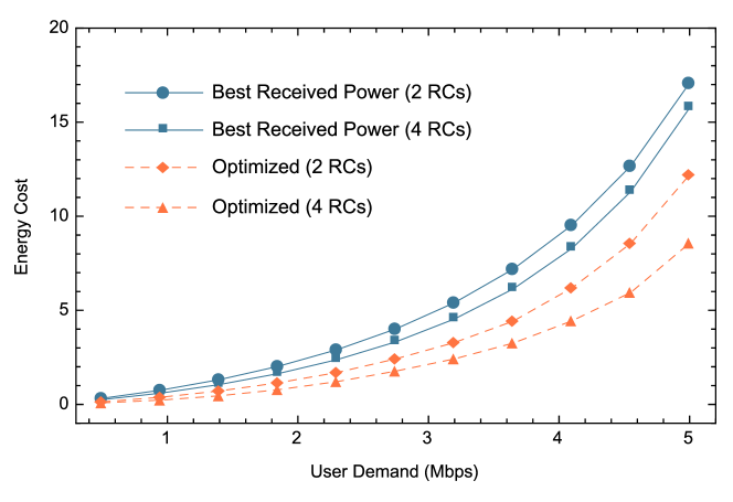
Figure 2: User demand versus energy cost.

In Figure 2, there are two network scenarios, in which 2 and 4 RCs are deployed in each hexagonal region, respectively. As references for comparison, each UE (or RC) $j$ is associated with the cell in $\mathcal{C}_{j}$ with the best received power. As expected, the 4-RCs case benefits more on energy performance via relay selection, compared to the 2-RCs case, since that each UE has more options for choosing its serving cell in the former. For these two cases, the improvements by using the proposed algorithm are $34\%$ and $47\%$, respectively. Furthermore, the improvement becomes larger, with the increase of the user demand, which indicates that an appropriate relay selection is crucial for a network with heavy data traffic. We remark that for the best-received power based relay selection, the network can still also benefit from deploying more RCs on energy cost. In other words, the energy cost can be reduced by deploying more RCs, without optimizing the relay selection. However, one can see from the numerical results that the corresponding gain is far less compared to optimizing the relay selection.

VII Conclusion

This paper has provided insights as well as an algorithm for energy-aware relay selection in load-coupled OFDMA cellular networks. The algorithm exhibits good performance for energy saving.

References

- [1] J. G. Andrews, S. Buzzi, W. Choi, S. V. Hanly, A. Lozano, A. C. K. Soong, and J. C. Zhang, “What will 5G be?” IEEE Journal on Selected Areas in Communications, vol. 32, no. 6, pp. 1065–1082, 2014.
- [2] D. S. Michalopoulos, H. A. Suraweera, and R. Schober, “Relay selection for simultaneous information transmission and wireless energy transfer: A tradeoff perspective,” IEEE Journal on Selected Areas in Communications, vol. 33, no. 8, pp. 1578–1594, 2015.
- [3] Z. Sheng, J. Fan, C. H. Liu, V. C. M. Leung, X. Liu, and K. K. Leung, “Energy-efficient relay selection for cooperative relaying in wireless multimedia networks,” IEEE Transactions on Vehicular Technology, vol. 64, no. 3, pp. 1156–1170, 2015.
- [4] “5g radio access,” Ericsson, Tech. Rep., 2014.
- [5] M. Dohler, T. Nakamura, A. Osseiran, J. F. Monserrat, O. Queseth, and P. Marsch, 5G Mobile and Wireless Communications Technology. Cambridge University Press, 2016.
- [6] “3gpp tr 36.116,” 3GPP, Tech. Rep. V13.0.1, 2016.
- [7] J. Gora and S. Redana, “In-band and out-band relaying configurations for dual-carrier LTE-advanced system,” in Proceedings of IEEE PIMRC, 2011, pp. 1820–1824.
- [8] R. L. G. Cavalcante, S. Stanczak, M. Schubert, A. Eisenblaetter, and U. Tuerke, “Toward energy-efficient 5G wireless communications technologies: Tools for decoupling the scaling of networks from the growth of operating power,” IEEE Signal Processing Magazine, vol. 31, no. 6, pp. 24–34, 2014.
- [9] C. K. Ho, D. Yuan, L. Lei, and S. Sun, “Power and load coupling in cellular networks for energy optimization,” IEEE Transactions on Wireless Communications, vol. 14, no. 1, pp. 509–519, 2015.
- [10] I. Siomina and D. Yuan, “Analysis of cell load coupling for lte network planning and optimization,” IEEE Transactions on Wireless Communications, vol. 11, no. 6, pp. 2287–2297, 2012.
- [11] “3gpp tr 36.913,” 3GPP, Tech. Rep. V13.0.0, 2016.
- [12] R. D. Yates, “A framework for uplink power control in cellular radio systems,” IEEE Journal on Selected Areas in Communications, vol. 13, no. 7, pp. 1341–1347, 1995.
- [13] “3gpp tr 36.814,” 3GPP, Tech. Rep. V9.0.0, 2010.