Tomographic reflection modelling of quasi-periodic oscillations in the black hole binary H 1743–322

Abstract

Accreting stellar mass black holes (BHs) routinely exhibit Type-C quasi-periodic oscillations (QPOs). These are often interpreted as Lense-Thirring precession of the inner accretion flow, a relativistic effect whereby the spin of the BH distorts the surrounding space-time, inducing nodal precession. The best evidence for the precession model is the recent discovery, using a long joint XMM-Newton and NuSTAR observation of H 1743–322, that the centroid energy of the iron fluorescence line changes systematically with QPO phase. This was interpreted as the inner flow illuminating different azimuths of the accretion disc as it precesses, giving rise to a blue/red shifted iron line when the approaching/receding disc material is illuminated. Here, we develop a physical model for this interpretation, including a self-consistent reflection continuum, and fit this to the same H 1743–322 data. We use an analytic function to parameterise the asymmetric illumination pattern on the disc surface that would result from inner flow precession, and find that the data are well described if two bright patches rotate about the disc surface. This model is preferred to alternatives considering an oscillating disc ionisation parameter, disc inner radius and radial emissivity profile. We find that the reflection fraction varies with QPO phase ($3.5\sigma$), adding to the now formidable body of evidence that Type-C QPOs are a geometric effect. This is the first example of tomographic QPO modelling, initiating a powerful new technique that utilizes QPOs in order to map the dynamics of accreting material close to the BH.

1 Introduction

In black hole (BH) X-ray binary systems, matter is accreted from the binary partner through a geometrically thin, optically thick disc, which emits a multi-coloured blackbody spectrum (Shakura & Sunyaev 1973; Novikov & Thorne 1973). Compton up-scattering of soft seed photons by a cloud of hot electrons close to the black hole also contributes a power-law component to the X-ray spectrum, with low and high energy cut-offs determined respectively by the seed photon and electron temperatures (Thorne & Price 1975; Sunyaev & Truemper 1979). Some fraction of the Comptonized photons reflect from the disc and are scattered into our line-of-sight. This imprints characteristic reflection features onto the spectrum, including a prominent iron K_α fluorescence line at $\sim 6.4$ keV and a so-called reflection hump, resulting from inelastic free-electron scattering, peaking at $\sim 30$ keV (Ross & Fabian 2005; García et al. 2013). These reflection features provide the opportunity to probe the dynamics of the accretion disc, since the iron line is observed to be distorted by Doppler shifts from orbital motion and gravitational redshift (Fabian et al. 1989).

So-called Type-C quasi-periodic oscillations (QPOs) are routinely observed in the X-ray flux, with the oscillation frequency increasing from $\sim 0.1-30$ Hz as the spectrum transitions from the hard power-law dominated hard state to the disc dominated soft state (e.g. Wijnands et al. 1999). In the truncated disc model, the disc evaporates inside of some transition radius to form a power-law emitting hot inner flow (Ichimaru 1977; Done et al. 2007). The spectral transitions then arise as the disc inner radius moves inwards, until it reaches the innermost stable circular orbit (ISCO) in the soft state. Alternatives include a corona partially covering the disc, confined by magnetic fields (Galeev, Rosner & Vaiana 1979; Haardt & Maraschi 1991) and an outflowing jet (Markoff et al. 2005). In all models, changes to the accretion geometry are required to explain the spectral transitions.

Suggested QPO mechanisms in the literature either consider instabilities in the accretion flow (e.g.Tagger & Pellat 1999; Cabanac et al. 2010), or a geometric oscillation (e.g. Stella & Vietri 1998; Wagoner et al. 2001). There is now strong evidence in favour of the geometric models, since high inclination (more edge-on) systems display stronger QPOs than low inclination (more face-on) systems (Schnittman et al. 2006; Motta et al. 2015; Heil et al. 2015). Phase lags between energy bands also strongly depend on inclination, with hard photons lagging soft for low inclination objects, and vice-versa for high inclination objects (van den Eijnden et al, submitted). A prominent interpretation associates the QPO with Lense-Thirring precession (Stella & Vietri 1998). This is a General Relativistic effect whereby the spin of the BH induces precession in orbits of particles inclined relative to the equatorial plane (Lense & Thirring 1918). Schnittman, Homan & Miller (2006) considered a precessing ring at the inner edge of the disc. However, the disc is expected to be held stationary by viscosity (Bardeen & Petterson 1975), and the QPO amplitude is stronger in the Comptonized spectrum than in the disc spectrum (Sobolewska & Życki 2006; Axelsson et al. 2014). Ingram, Done & Fragile (2009) instead suggested that the entire inner flow precesses whilst the disc remains stationary, motivated by the simulations of Fragile et al. (2007).

Ingram & Done (2012b) showed that precession of the inner flow will cause the iron line to rock from blue to red shifted, as the inner flow illuminates the approaching followed by receding disc material. This prediction can be directly tested with QPO phase-resolved spectroscopy. Phase-resolving poses a technical challenge, since the stochastic nature of the QPO prevents phase folding - as can be used for e.g. neutron star pulses (e.g. Wilkinson et al. 2011; Gierliński et al. 2002) - from being appropriate. Miller & Homan (2005) applied a simple flux selection to strong QPOs from GRS 1915+105, but constraining spectra for more than two phases requires a more sophisticated method. Ingram & van der Klis (2015, hereafter IK15) developed a technique that uses the average Fourier properties in order to reconstruct phase-resolved spectra, and used it to discover spectral pivoting in GRS 1915+105. Stevens & Uttley (2016) used a similarly sophisticated technique in order to measure changes in the disc temperature of GX 339-4 during the QPO cycle (although this is for a Type B QPO; see e.g. Casella et al. 2005 for QPO classifications). However, the phase-resolved behaviour of the iron line could not be constrained in these studies due to limitations on data quality. Ingram et al. (2016, hereafter I16) applied a developed version of the IK15 method to a long XMM-Newton and NuSTAR observation of H 1743–322 in the hard state in order to measure a QPO phase dependence of the iron line centroid energy. This provides strong evidence that the QPO is driven by precession - either precession of the inner flow (Ingram & Done 2012b), or alternatively of the disc (i.e. precession of the reflector; Schnittman et al. 2006).

In this paper, we develop a physical model for the QPO phase-resolved spectra measured in I16. Our model is designed to mimic illumination of the disc by a precessing inner flow - as the flow precesses, it preferentially illuminates different azimuths of the disc. Rather than consider a specific geometry for the precessing flow, we parameterise the asymmetric, rotating illumination profile with an analytic function. This has the advantage of making no a priori assumptions about the inner flow geometry, it enables the model to be fast enough to fit directly to data, and it allows us to define asymmetry parameters that can be set to zero in order to recover the usual case of axisymmetric illumination. In Section 2 we summarise the observations and the phase-resolving method. In Section 3, we fit the time-averaged spectrum with a relativistic reflection model in order to address cross-calibration issues between XMM-Newton and NuSTAR, and also to provide a comparison to our eventual tomographic modelling. We present the details of our model in Section 4 and the results of our tomographic modelling in Section 5. We discuss our results in Section 6 and present our conclusions in Section 7.

2 Data analysis

2.1 Observations

We consider XMM-Newton and NuSTAR data from the 2014 outburst of H 1743–322. XMM-Newton observed this outburst for two full orbits around the Earth in late September 2014. We use data from the EPIC pn, which was in timing mode for the entire exposure. The first orbit has obs ID 0724400501, and the second orbit is split into two obs IDs (0724401901 and 0740980201) due to a change in PI. In I16, we split the XMM-Newton data into four segments: orbit 1a, orbit 1b, orbit 2a and orbit 2b (see Fig. 1 in I16). This was to allow for a minor change in instrumental setup between orbits 2a and 2b, and for possible changes in the source geometry over the course of orbit 1. We employ the same naming conventions in this paper. NuSTAR observed the source (obs ID 80001044004) simultaneous with the second XMM-Newton orbit. We use data from both of the NuSTAR focal plane modules, FPMA and FPMB. Here, we use exactly the same data reduction procedure described in I16.

In this paper, we use only the NuSTAR data and the orbit 2 XMM-Newton data. We keep the data for orbits 2a and 2b separate, but tie together parameters in our fits between the two XMM-Newton segments and the NuSTAR exposure. We exclude orbit 1 for a number of reasons. Firstly, there is no simultaneous NuSTAR coverage. It is very useful to jointly fit XMM-Newton and NuSTAR data, since XMM-Newton provides high signal-to-noise at the iron line and NuSTAR gives a view of the reflection hump. Unfortunately, there are some cross-calibration issues between XMM-Newton and NuSTAR, which we will discuss in the following Section. We show that these issues can be overcome if data from the two observatories are simultaneous, but without this simultaneity it is ambiguous whether differences in the spectrum are down to cross-calibration, or genuinely down to evolution of the spectrum between the two observations. Secondly, we saw in I16 that orbits 1a, 2a, 2b and the NuSTAR observation all showed the same characteristic modulation in line energy with QPO phase, with maxima at $\sim 0.2$ and $\sim 0.7$ cycles, whereas orbit 1b showed a different modulation. The reason behind this difference is still not clear, so we exclude the anomalous data set, and also orbit 1a to avoid simply ‘cherry picking’ the best data.

2.2 Summary of phase-resolving method

The phase-resolving method used is described extensively in I16 and IK15. Here, we summarise the method and leave the details to earlier references. Conceptually, the method consists of constraining the average QPO Fourier transform (FT) for each energy channel. That is, for each energy channel, we wish to measure the mean count rate, and the amplitude and phase of each observed QPO harmonic. We detect only the fundamental (first harmonic) and the overtone (second harmonic) over the broad band noise, and so cannot consider any higher harmonics. The zeroth harmonic is simply the mean count rate, and also needs to be taken into consideration. Since the mean count rate is real, it trivially has a phase of zero. Therefore, for a given energy channel, the QPO FT consists of five numbers: the (amplitude of the) mean count rate, the amplitude of the first and second harmonics, and the phase of the first and second harmonics. Equivalently, we can think in terms of real and imaginary parts instead of amplitude and phase, in which case the five numbers are: the real part of the mean count rate, first and second harmonics and the imaginary part of the first and second harmonics.

It is fairly straight forward to measure the amplitude of the two QPO harmonics as a function of energy. The simplest way is to make a power spectrum for each energy channel and fit each power spectrum with a sum of Lorentzian functions. The squared amplitude of the $j$th harmonic is simply the integral of the Lorentzian component representing it. We used a slightly more complicated method in I16 to maximize signal-to-noise and to circumvent the NuSTAR deadtime but, conceptually, our method is the same as described here. The phase can be measured by defining a reference band, and, for each energy channel, calculating the cross-spectrum between that channel (the subject channel) and the reference band (van der Klis et al. 1987; Uttley et al. 2014). The phase of the cross-spectrum averaged over the width of the $j$th harmonic tells us by how many radians the $j$th harmonic of the subject channel lags the $j$th harmonic of the reference band. However, we instead want to know by how many radians the $j$th harmonic of the subject channel lags the first harmonic of the reference band. To know this, we must measure the phase difference between the first and second harmonics in the reference band, and use this to correct the phase as measured from the cross-spectrum. We measure this phase difference between harmonics using the method of IK15.

With the QPO FT as a function of energy constrained, we can proceed in two ways. The simplest is to inverse FT the data, to give a waveform for each energy channel. It is simple to picture this: the waveform for a given channel is a constant (the mean count rate of that channel) plus two sine wave functions of QPO phase representing the two harmonics, each with their own amplitude and phase. Having a waveform for each energy channel, we can simply take the spectrum for different values of QPO phase and fit each phase with a spectral model, and see how the parameters of the spectral model change with QPO phase. However, the statistics are badly behaved in this case. This is because, even though the five numbers per energy channel that make up the QPO FT do have well-behaved, Gaussian errors, the inverse FT introduces correlations between QPO phases. It is therefore much cleaner from a statistical point of view to define a model for how the spectrum changes as a function of QPO phase, and then FT the model. Note that both of these methods are equivalent - we can either inverse FT the data and fit in the time domain, or we can FT the model and fit in the Fourier domain. The only difference is that the Fourier domain method is superior when it comes to assessing goodness of fit, error calculations etc. Therefore, in this paper, we fit entirely in the Fourier domain.

3 Time-averaged spectral fits

Before analysing the QPO FT, we first fit the time-averaged XMM-Newton and NuSTAR spectra with a relativistic reflection model. One motivation for this is to gain insight into the effect of spectral variability on the time-averaged spectrum. If spectral variability were exclusively linear, the QPO phase-averaged spectrum would be exactly equal to the spectrum calculated using the phase-averaged spectral parameters. However, we saw in I16 that the iron line centroid energy and the photon index change systematically with QPO phase. These changes are mildly non-linear and therefore may introduce biases into time-averaged spectral modelling. Another motivation is to explore the cross-calibration discrepancy between XMM-Newton and NuSTAR. The XMM-Newton spectrum is significantly harder than the NuSTAR spectrum.

Table 1: Best fit parameter values and $1\sigma$ errors for our time-averaged spectral fit. $\Delta\Gamma$ is a calibration parameter that accounts for the offset in spectral index measured by XMM-Newton and NuSTAR. $R_{g}$ is a gravitational radius, $R_{g}=GM/c^{2}$. See the text for more details.

Parameter	$\Delta\Gamma$	$\Gamma$	$r_{\rm in}$	$i$	$E_{\rm cut}$	$\log_{\rm 10}\xi$	$f$	$A_{\rm Fe}$
Units			$R_{g}$	deg	keV		$\%$
Best fit	$0.22$	$1.57$	$36.3$	$67.5$	$285.0$	$2.0$	$24.7$	$0.7$
$1\sigma$ error	$5\times 10^{-4}$	$10^{-3}$	$4.1$	$2.3$	$6.4$	$5\times 10^{-2}$	$0.3$	$3\times 10^{-2}$

We consider XMM-Newton orbit 2a and select a strictly simultaneous interval of the NuSTAR observation. We use xspec v12.8.2 to fit the model

$$constant~{}\times~{}E^{\Delta\Gamma}~{}\times~{}tbabs~{}\times~{}[~{}relxill~{}+~{}xillver~{}],$$ (1)

to the FPMA, FPMB ($4-75$ keV) and EPIC pn ($4-10$ keV) spectra simultaneously. We choose to ignore the $<4$ keV range in the XMM-Newton data in order to avoid calibration features resulting from uncertain modelling of the so-called charge transfer inefficiency (see De Marco & Ponti 2016 and references therein for a discussion on this). The $>4$ keV energy range also reliably has a negligible contribution from direct disc emission, with the disc temperature for this observation measured to be $T_{\rm in}<0.4$ keV by both Stiele & Yu (2016) and De Marco & Ponti (2016). The constant factor simply accounts for differences in absolute flux calibration. We introduce the parameter $\Delta\Gamma$ to account for the discrepancy in photon index measured individually for the two observatories. We fix $\Delta\Gamma=0$ for both NuSTAR modules, and allow it to go free for the pn. We choose to fit this way around for a number of reasons. Firstly, the reflection models we use are only tabulated for $\Gamma\geq 1.4$, so using the raw XMM-Newton spectrum, which is very hard, risks going close to this boundary at some point during the running of the $\chi^{2}$ minimisation algorithm. Secondly, the XMM-Newton spectrum is far harder than is commonly observed in the hard state (see e.g. Shaposhnikov & Titarchuk 2009), whereas the photon index measured from the NuSTAR spectrum is consistent with expectation. Finally, it has previously been reported that the pn in timing mode also measures a harder power-law index than RXTE for a hard state observation of GX339-4 similar in flux and spectral shape to the observations analysed here (Kolehmainen et al. 2014). We tie all other parameters to be the same for the two observatories.

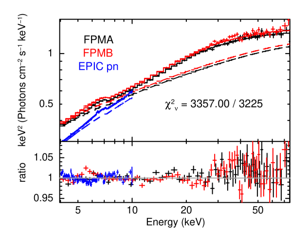
Figure 1: Unfolded time-averaged spectrum with the best fit model (top) and data to model ratio (bottom). We consider XMM-Newton orbit 2a and the strictly simultaneous portion of the NuSTAR observation. FPMA, FPMB and EPIC-pn data and corresponding models are as labelled. The dashed lines represent the continuum model. The pn spectrum is significantly harder than the NuSTAR spectra, but we are able to find an acceptable fit using a multiplicative correction factor (equation 1). Data have been re-binned for plotting purposes

$Tbabs$ accounts for interstellar absorption, and we freeze the hydrogen column density to $N_{h}=2\times 10^{22}{\rm cm}^{-2}$ assuming the abundances of Wilms, Allen & McCray (2000), following other spectral analyses of the same data set (De Marco & Ponti 2016; Stiele & Yu 2016). This is slightly higher than the value used in I16, but we find that it has no significant effect on the measurement of an iron line centroid energy modulation. $Relxill$ is a relativistic reflection model which includes an exponentially cut-off power-law X-ray continuum and a reflection component which is smeared by the orbital motion of disc material and gravitational redshift (García et al. 2014). We include the $xillver$ component (García et al. 2013), which is the same as $relxill$ but without the relativistic smearing, to account for a distant reflector which it is possible to detect in XMM-Newton spectra of BH X-ray binaries in the form of a narrow iron line (e.g. Cygnus X-1: Fabian et al. 2012; GX 339-4: Kolehmainen et al. 2014). The shape of the rest-frame reflection spectrum depends on the shape of the illuminating continuum, the disc ionisation parameter $\log_{10}\xi$ and the iron abundance relative to solar, $A_{Fe}$. For the $relxill$ component, we allow $\log_{10}\xi$ and $A_{Fe}$ to be free parameters. For the distant reflector, we assume neutral material ($\log_{10}\xi=0$), with the same iron abundance as the $relxill$ component. The relativistic smearing depends on the inclination angle $i$, the disc inner radius $r_{\rm in}$ and the radial dependence of illuminating flux, which we assume to be $\propto r^{-3}$. Since we do not assume that $r_{\rm in}$ is equal to the innermost stable circular orbit (ISCO), the relativistic smearing only depends very weakly on the BH spin parameter, $a$ (the energy shifts and photon paths both depend on the metric). For this reason, we fix $a=0.21$ to be consistent with the measurement of $a\approx 0.2$ made by Steiner et al. (2012) through disc spectral fitting and the limit $a\gtrsim 0.2$ placed by Ingram & Motta (2014) using high frequency QPOs.

Fig 1 shows the data unfolded around the best-fit model (top) and the ratio of data to model (bottom). After applying $0.5\%$ systematic errors to account for uncertainties in the telescope response matrices (as is widely practiced: e.g. Kolehmainen et al. 2014; Plant et al. 2015), we achieve an acceptable fit (reduced $\chi^{2}=3357/3225=1.04$). We find through an F-test that the distant reflector is formally required with a significance of $5.3\sigma$ (since the best-fit without the $xillver$ component has a reduced $\chi^{2}=3387/3226$). Table 1 shows the resulting best-fit parameters with $1\sigma$ errors. Our best fit model indicates that the disc is truncated outside of the ISCO and yields a moderately high inclination, consistent with the source showing dips but not eclipses (Homan et al. 2005). Steiner et al. (2012) measured the angle between our line of sight and the radio jet (which is likely aligned with the BH spin axis; Blandford & Znajek 1977) in H 1743–322 to be $\sim 75^{\circ}$. Thus, although the two angles are broadly consistent within errors, there is room for a modest misalignment between the disc and BH spin axes, as is required for the precession model. The fit indicates a fairly low ionisation, consistent with the relatively low continuum luminosity, and a mildly sub-solar iron abundance.

4 Tomographic model

Figure 2: Left: Ray traced disc images for two QPO phases (as labelled) visualising our best fit model. The disc inner radius and inclination are equal to our best fit values, and the border of the multi-coloured patches is set by the best fit illumination profile for the relevant QPO phase. The colour scheme of the multi coloured patches encodes blue shifts. Right: The best fitting reflection spectrum, zoomed in on the iron line, for the same QPO phases. The QPO phase = $0.2$ cycles iron line (blue) has a boosted blue horn and red wing because the blue and red shifted parts of the disc are preferentially illuminated (top image), in contrast to the QPO phase = $0.4$ iron line (red line), which corresponds to the bottom disc image. Animated versions of these plots can be viewed at and downloaded from https://figshare.com/articles/Tomographic_modelling_of_H_1743-322/3503933. These animations are designed to be played together.

In this section, we describe our physical model for the QPO phase-resolved reflection spectrum. The intention is to mimic the asymmetric, rotating illumination pattern that would be caused by a precessing inner flow irradiating the disc by using an analytic parameterisation which we can fit directly to the data. The bright patches on the disc in Fig. 2 illustrate this for two QPO phases. We represent the reflected intensity as a function of disc radius $r$, disc azimuth $\phi$, and QPO phase $\gamma$ using the function

$$I_{E_{e}}(r,\phi,\gamma)\propto r^{-q} \Big{\{}1+A_{1}\cos^{2}\left[(\gamma-\phi+\phi_{1})/2\right]$$ (2)

$$+ A_{2}\cos^{2}\left[\gamma-\phi+\phi_{2}\right]\Big{\}}I_{E_{e}},$$

where $I_{E_{e}}$ is the rest-frame reflection spectrum and $I_{E_{e}}(r,\phi,\gamma)$ is the specific intensity of radiation emitted at photon energy $E_{e}$ for a given patch of the disc at a given QPO phase. We see that the intensity is a power-law function of radius, the same as our fits to the time-averaged spectrum in Section 3 (with $q=3$). We define the z-axis to be parallel with the disc rotation axis such that the disc lies in the x-y plane. The disc azimuth $\phi$ is measured clockwise from the x-axis, which is defined as the projection of the observer’s line-of-sight on the black hole equatorial plane. The dependence of intensity on disc azimuth is parameterised through the cosine terms in equation 2. Setting $A_{2}=0$, $A_{1}>0$ creates only one bright patch that rotates about the disc surface once per precession cycle, leading to only one maximum in the iron line energy per QPO cycle. At QPO phase $\gamma=0$, the brightest patch of the disc in this case would be $\phi=\phi_{1}$. Setting $A_{1}=0$, $A_{2}>0$ corresponds to the front and back of the flow irradiating the disc with equal intensity, leading to two identical patches rotating about the disc surface and two identical maxima in the line energy per QPO cycle. At QPO phase $\gamma=0$, the two brightest patches of the disc in this case would be $\phi=\phi_{2}$ and $\phi=\phi_{2}+180^{\circ}$. In I16, we observed two maxima in the iron line centroid energy per QPO cycle with the second slightly higher than the first, thus the best fit model will likely have $A_{1}>0$, $A_{2}>0$. This indicates that the front and back of the flow irradiate the disc, and thus requires the flow to have a fairly small vertical extent (or alternatively the misalignment between disc and flow is large). Ingram & Done (2012b) instead modelled the flow as an oblate spheroid with large vertical extent, and therefore the underside of the flow was never above the disc mid-plane. The cosines in equation 2 are squared so as to prevent the possibility of unphysical parameter combinations for which the intensity is negative.

The specific flux observed at energy $E_{o}$ from a patch of the disc subtending solid angle $d\Omega(r,\phi)$ to the observer is

$$dF_{E_{o}}(r,\phi,\gamma)=(E_{o}/E_{e})^{3}I_{E_{e}}(r,\phi,\gamma)d\Omega(r,\phi).$$ (3)

Each solid angle element $d\Omega(r,\phi)$ can be seen as a pixel on the observer’s camera. We define a $400\times 400$ circular (polar) grid of pixels and, for each one, trace the unique null-geodesic in the Kerr metric (using the code geokerr; Dexter & Agol 2009) back from the centre of the pixel to assess if and where that geodesic intercepts the disc. The blue shift, $(E_{o}/E_{e})$, is calculated for all the photon paths that intercept the disc using the equation

$$\frac{E_{o}}{E_{e}}=\frac{\sqrt{-g_{tt}-2g_{t\phi}\omega-g_{\phi\phi}\omega^{2}}}{1+\omega\alpha\sin(i)},$$ (4)

where $g_{\mu\nu}$ is the Kerr metric, $\omega=1/(r^{3/2}+a)$ is the angular velocity in dimensionless units, and the impact parameter $\alpha$ is the horizontal distance from the centre of the observer’s camera to the centre of the pixel in $R_{g}$. We use the same coordinate system and ray-tracing procedure as Middleton & Ingram (2015) except here we assume clockwise (left-handed) rotation so that blue shifts are always to the right and red shifts are always to the left both for disc images and spectra (see Fig. 2). Equation 4 assumes disc rotation in the BH equatorial plane. This is not true if there is a misalignment between disc and BH rotational axes, as we are imagining here, but the error introduced is very small (Ingram et al. 2015). We use $xillver$ (García et al. 2013) for the rest-frame reflection spectrum, $I_{E_{e}}$ (see section 3).

We allow the continuum normalisation $N$, the reflection fraction $f$, and the photon index, $\Gamma$ to vary as a function of QPO phase, $\gamma$, with two non-zero harmonics. For example, the photon index varies with QPO phase as

$$\Gamma(\gamma)=\Gamma_{0}+A_{1\Gamma}\sin[\gamma-\phi_{1\Gamma}]+A_{2\Gamma}\sin[2(\gamma-\phi_{2\Gamma})],$$ (5)

and we use analogous expressions for the other two variable parameters, $N(\gamma)$ and $f(\gamma)$.

Our model calculates the integrated specific flux as a function of observed energy $F_{E_{o}}(\gamma)$ for 16 steps in $\gamma$ and, for each energy channel, calculates the FT $\tilde{F}_{E_{o}}(j)$ for the harmonics $j=0$, $j=1$ and $j=2$. The $j=0$ harmonic (the so-called DC component) is simply the spectrum averaged over all $\gamma$. Each harmonic has real and imaginary parts, but the imaginary part of the DC component is trivially zero. This leaves five spectra to fit simultaneously to the observed QPO FT. We load our model into xspec using the local model functionality. We include absorption using $tbabs$ for real and imaginary parts of every harmonic (since absorption is multiplicative). We also add a distant reflector ($xillver$) to the DC component only, since a constant additive component does not contribute to the non-zero harmonics. As discussed in I16, the fact that we fit in terms of real and imaginary parts rather than amplitude and phase means that the instrument response is trivially accounted for when the data are loaded into xspec. In order to avoid edge effects of the convolution, we extend the energy grid used to calculate the model up to $200$ keV (using the xspec command ‘$energies~{}extend~{}high~{}200$’).

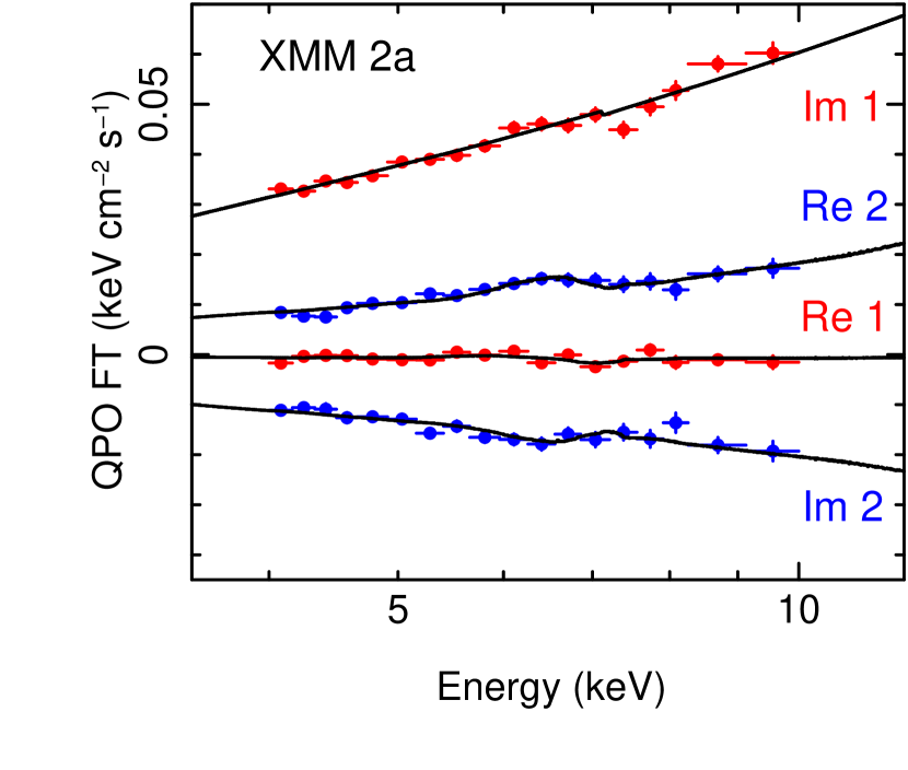
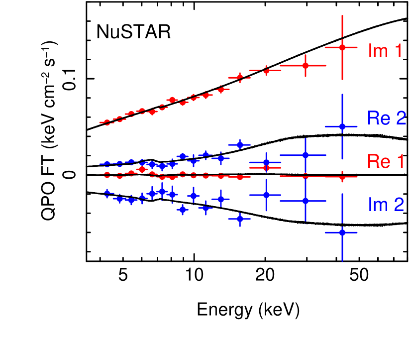
Figure 3: QPO FT as a function of energy for XMM-Newton orbit 2a (left) and NuSTAR (right). Real and imaginary parts of the first and second harmonics are as labelled. Real and imaginary parts of the data are colour coded blue and red respectively, and the black lines depict the best fitting model. The data are unfolded around the best fitting model and are in units of energy squared $\times$ specific photon flux. We see features around the iron line and reflection hump, particularly for the real parts. XMM-Newtonand NuSTARshow the same trends.

5 Results

We load the model described in the previous section into xspec as the local model $modfeprec$. We fit to the measured energy dependent FT of the QPO, considering the real and imaginary parts of the first and second harmonics, and also the time-averaged spectrum (which is the real part of the zeroth harmonic). Altogether, this gives five spectra to simultaneously fit for each data set. For the non-zero harmonics, we use the same coarse binning employed in I16, which is necessary to ensure Gaussian errors. For the zeroth harmonic (the time-averaged spectrum), we instead use the fine spectral binning employed here in Section 3 (although note that this is still coarser than the instrument response). As a check, we also performed fits using coarse binning for the time-averaged spectrum and see no significant differences in our best-fit parameters or goodness of fit. We use the fine binning for our analysis, however, since it is sensitive to parameter combinations that can reproduce the observed variability properties but predict sharp features in the time-averaged spectrum that are not observed.

We employ the model

$$constant~{}\times~{}E^{\Delta\Gamma}~{}\times~{}tbabs~{}\times~{}[~{}modfeprec~{}+~{}xillver~{}],$$ (6)

where $modfeprec$ outputs either the real or imaginary part of the first, second or zeroth QPO harmonic. We fix the calibration parameters ($constant$ and $\Delta\Gamma$) to the values obtained in Section 3, and continue to use $N_{h}=2\times 10^{22}$ cm^-2 for the hydrogen column density. We also fix the ionisation parameter, high energy cut-off and relative iron abundance to the values obtained in Section 3. The $xillver$ component, as before, accounts for distant reflection, which we assume not to vary on the QPO period and therefore set its normalisation to zero for all non-zero harmonics. We jointly fit for the two XMM-Newton observations and the NuSTAR observation. We tie all physical parameters between these three data sets, except for those describing the modulation of the continuum normalisation. As in I16, the modulation in the continuum normalisation is very similar for the three data sets, but can be measured to a high enough precision for small differences to be highly significant.

5.1 Best fit tomographic model

We achieve a good fit with reduced $\chi^{2}=2544.54/2511=1.013$ (rejection probability $68.5\%$). Fig. 3 shows the QPO FT data and model for XMM-Newton orbit 2a (left) and NuSTAR (right). Here, the real and imaginary parts of the first and second harmonics are as labelled, with real and imaginary data points colour coded respectively blue and red, and the model always plotted as a black line. The data are unfolded around the instrument response assuming the best fit model and are in units of energy squared $\times$ specific photon flux (i.e. the $eeuf$ option in xspec). We see curvature around the iron line, particularly for the real parts. In the NuSTAR data, we also see the effect of the reflection hump at high energy. In the model, these features result from changes in the shape of the reflection spectrum over a QPO cycle.

Table 2: Best fit parameters for our tomographic modelling. See the text for more details.

Parameter	$\Gamma_{0}$	$r_{\rm in}$	$i$	$f_{0}$	$A_{1}$	$A_{2}$	$\phi_{1}$	$\phi_{2}$
Units		$R_{g}$	deg	$\%$			deg	deg
$1\sigma$ upper	$1.571$	$37.30$	$73.33$	$23.20$	$2.263$	$8.740$	$138.685$	$28.105$
Best fit	$1.567$	$31.47$	$70.68$	$21.83$	$0.93$	$3.50$	$94.66$	$18.98$
$1\sigma$ lower	$1.563$	$27.81$	$67.51$	$20.48$	$0.322$	$1.275$	$49.675$	$8.93$

Table 2 shows our best-fit parameters with $1~{}\sigma$ errors. Fig. 2 shows a visualisation of the disc illumination profile indicated by the best-fit asymmetry parameters $A_{1}$, $A_{2}$, $\phi_{1}$ and $\phi_{2}$ (see equation 2). We show disc images for two QPO phases with the corresponding phase-resolved reflection spectra. The multi-coloured patches pick out where the illuminating intensity, $I_{E_{e}}(r,\phi,\gamma)$, is greater than $10\%$ of its maximum value, with the rest of the disc coloured grey. The colour coding of the patches encodes blue shifts (equation 4). The two QPO phases shown are $0.2$ cycles ($72^{\circ}$, blue line profile) and $0.4$ cycles ($144^{\circ}$, red line profile), since these roughly correspond respectively to the maximum and minimum line centroid energy, as measured by I16. For the purposes of these plots, the modulations in $\Gamma$, reflection fraction and normalisation have been set to zero, to ensure that all changes to the reflection spectrum result purely from changes to the disc illumination profile. All other parameters come directly from our best fitting model. We see that the line has a strongly boosted blue horn and a suppressed core (blue line) when the left and right sides of the disc are illuminated (top disc image). This is because we see enhanced emission from both the blue shifted approaching material and the red shifted receding material, but Doppler boosting ensures that the blue shifted emission dominates. In contrast, the line has a strong core but suppressed wings (red line) when the front and back of the disc are illuminated (bottom disc image), since there is no enhancement of the Doppler shifted emission from the approaching and receding disc material. As with the time-averaged fits, we measure a moderately truncated disc and a fairly high inclination angle. Light bending effects are evident in the disc images through apparent warping of the disc, but we do not consider ghost images, since photons on these paths will likely be scattered before reaching the observer. Animated versions of the plots shown in Fig 2 can be viewed at and downloaded from the link given in the caption.

Fig. 4 is a contour plot resulting from varying the asymmetry parameters $A_{1}$ and $A_{2}$. The contours represent $\Delta\chi^{2}=2.3$ (black), 6.18 (red) and 11.83 (green). These levels correspond to 1, 2 and 3 $\sigma$ for two degrees of freedom. We see that fairly large values of $A_{1}$ and $A_{2}$ return a $\chi^{2}$ value within 1$\sigma$ of the best-fit (black cross). This is because of the way the illuminating flux, $I_{E_{e}}(r,\phi,\gamma)$, is parameterised. We see from equation 2 that $I_{E_{e}}(r,\phi,\gamma)$ is a sum with three terms. The first term does not depend on QPO phase, whereas the second two do. Increasing $A_{1}$ and $A_{2}$ respectively increases the relative importance of the second and third terms with respect to the first. However, increasing $A_{2}$ from, e.g. $100$ to $1000$ makes a negligible difference, since the constant component changes from being $1\%$ to $0.1\%$ of the flux in this case. Our parameterisation is of course designed to investigate the effect of setting $A_{1}=A_{2}=0$, in which case there is no QPO phase dependence of the line profile in the model. We see that $A_{2}$ is better constrained than $A_{1}$ and that the point $A_{1}=A_{2}=0$ lies outside of the $3\sigma$ contour. However, these contours are for two degrees of freedom, and the point $A_{1}=A_{2}=0$ is a special point, in that setting $A_{1}=A_{2}=0$ renders the fit insensitive to $\phi_{1}$ and $\phi_{2}$. Following I16, we therefore use an F-test to compare our best fit (reduced $\chi^{2}=2544.54/2511$) with the null-hypothesis (reduced $\chi^{2}=2556.98/2515$). This indicates that the best-fit model is preferred with $2.40~{}\sigma$ confidence. Therefore, although we can say with $3.70\sigma$ confidence that the line centroid energy is modulated (I16), our analysis yields a lower significance for an actual asymmetric illumination profile. This is partly because here we necessarily use a more complex model for the iron line than a Gaussian, and therefore lose degrees of freedom. Also, small apparent shifts in the iron line profile can be driven by changes in the reflection continuum, caused by changes in the photon index (which our model automatically takes into account). Finally, we have been rather conservative in excluding XMM-Newton orbit 1.

As another visualisation of our results, Fig. 5 shows how various quantities / model parameters vary with QPO phase. Each panel is labelled with a statistical significance. For the top panel, this is the significance of asymmetric illumination as calculated above. For the other three panels, this is the significance with which the plotted parameter changes with QPO phase, calculated using an F-test comparing the best fitting model with an alternative fit whereby the parameter in question is forced to be constant. In order to make this plot, we run a Monte Carlo Markov Chain for our best fit model and, for each of the four panels, calculate a histogram for each of 512 QPO phases (see I16 for details). The chain has 125,000 steps and we burn the first 25,000. For the top panel, we compute the line profile as a function of QPO phase, $L(\gamma,E)$, assuming a $\delta$-function rest-frame iron fluorescence line at $6.4$ keV and define the centroid energy as

$$E_{\rm c}(\gamma)=\frac{\int_{0}^{\infty}EL(\gamma,E){\rm d}E}{\int_{0}^{\infty}L(\gamma,E){\rm d}E}.$$ (7)

We see that the centroid energy calculated in this way follows the same trend as the centroid of the Gaussian used in I16, with maxima at $\sim 0.2$ and $\sim 0.7$ cycles. The second panel shows the reflection fraction. We see that this is modulated with QPO phase ($3.52\sigma$). The significance is calculated from an F-test, and does not depend on the chain. Our model is normalised such that the observed reflected flux will be higher when the approaching disc material is preferentially illuminated, even if $f$ remains constant, because of Doppler boosting. Changes in $f$ therefore indicate variability in the reflected flux on top of this effect. We expect changes in the reflection fraction if the misalignment angle between the inner flow and disc changes throughout a precession cycle (Ingram & Done 2012b). The third panel shows a modulation in $\Gamma$, however this is not significant ($0.95\sigma$). This modulation in $\Gamma$ has a different phase to that measured by I16, with maxima at $\sim 0.4$ and $\sim 0.9$ cycles, compared with $\sim 0.3$ and $\sim 0.8$ cycles in I16. The significance of the $\Gamma$ modulation has also drastically reduced compared with I16. This is because we now include a full reflection model with a continuum rather than just a Gaussian iron line. Our results indicate that the observed changes in spectral hardness during a QPO cycle are more due to changes in reflection fraction than photon index. An increase in reflection fraction makes the spectrum harder (since the reflected continuum is harder than the directly observed continuum). With no reflected continuum in the model, this hardening can only be modelled as a reduction in $\Gamma$. We can see evidence of this in Fig. 5, since the lowest reflection fraction ($\sim 0.25$ cycles) coincides with the highest $\Gamma$ in I16. The NuSTAR data is particularly important for constraining this, since the reflection hump gives a good constraint on the reflected continuum.

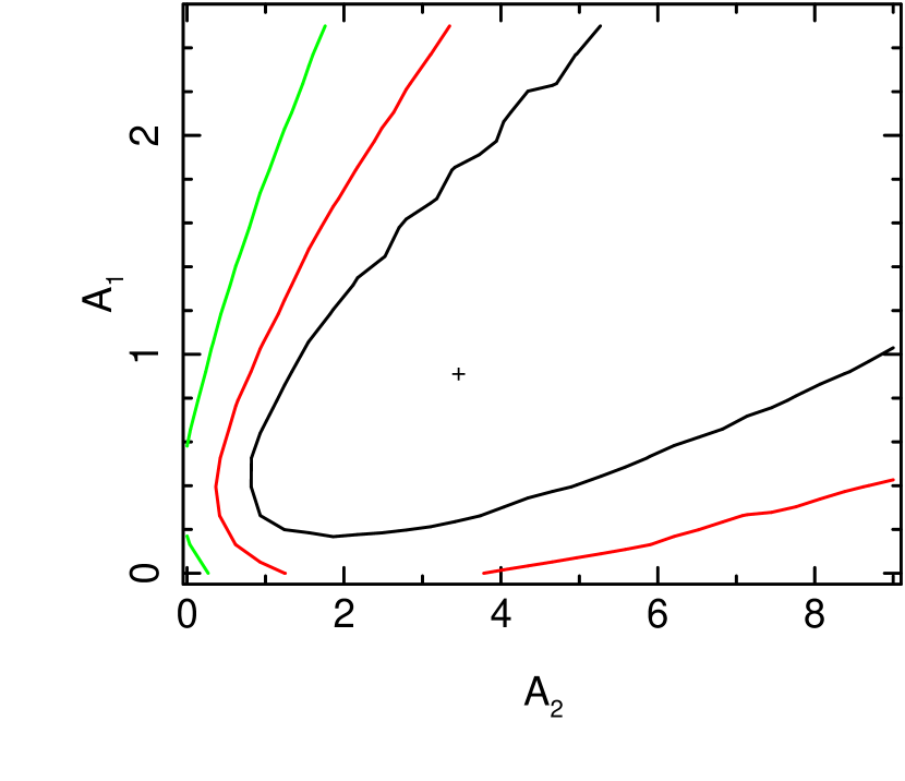
Figure 4: $\chi^{2}$ contour plot showing the two asymmetry parameters $A_{1}$ and $A_{2}$. The contours correspond to 1 (black), 2 (red) and 3 (green) $\sigma$ confidence for two degrees of freedom.

For completeness, we briefly investigate the anomalous XMM-Newton orbit 1b. In I16, we found that the best-fit iron line centroid energy modulation was very different in this data set to all the others, and also that the modulation was not statistically significant (see Fig. 7 in I16). As expected, when we fit these data with our tomographic model, the asymmetry parameters $A_{1}$ and $A_{2}$ are poorly constrained, and the best-fit model with $A_{1}=0.96$ and $A_{2}\approx 0$ is preferred to $A_{1}=A_{2}=0$ with a significance of only $0.5\sigma$. The absence of simultaneous NuSTAR data for this data set adds to the difficulty in constraining model parameters. Our best fitting value of $A_{2}\approx 0$ is consistent with the results of I16, who found that the best fitting iron line centroid energy modulation had no second harmonic (i.e. $A_{2E}\approx 0$). Our best fitting value of $\phi_{1}=160.9^{\circ}$ is also consistent with the I16 results, since this implies that the line centroid energy peaks at $\sim 0.5$ QPO cycles (see Fig. 7 in I16) - very different to the other data sets.

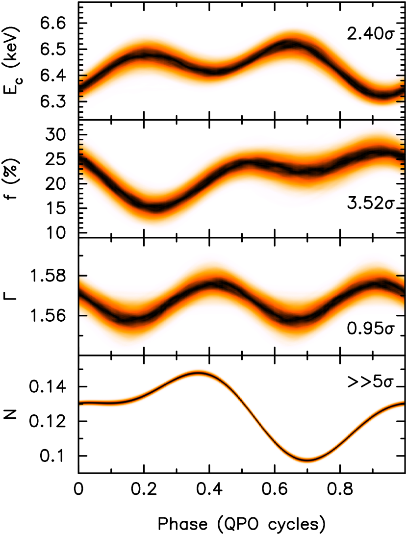
Figure 5: Visualisation of our best fitting parameter modulations. The iron line centroid energy, defined by equation 7, shows a characteristic variation with QPO phase, with two maxima at $\sim 0.2$ and $\sim 0.4$ cycles. This is the same trend as is presented in I16 for a Gaussian iron line model. We also see that the reflection fraction is modulated ($3.52\sigma$) and the photon index modulation is not statistically significant. The modulation in normalisation corresponds to XMM-Newton orbit 2a.

5.2 Alternative models

We also consider alternative interpretations for the iron line centroid energy modulation.

5.2.1 Modulated ionisation parameter

We first consider changes in the ionisation parameter, $\log_{10}\xi$, over a QPO cycle. An increase in ionisation leads to a higher rest-frame line energy, since the ions are on average more tightly bound (Matt et al. 1993; Done 2010). Therefore, it is possible, in principle, for there to be a modulation in line energy with no geometric changes. In this case, the disc ionisation should peak when the irradiating flux peaks, since it is the intensity of incoming radiation that governs the ionisation balance. Thus, we would expect in this case that the line energy should be in phase with the continuum flux, which is not the case (Fig. 5). Nonetheless, we test the ionisation hypothesis without this constraint. We set $A_{1}=A_{2}=0$ and parameterise the ionisation parameter as a function of QPO phase, $\log_{10}\xi(\gamma)$, in the same way as $\Gamma(\gamma)$ in equation 5, with the average, amplitudes and phases replaced by $\log_{10}\xi_{0}$, $A_{1\xi}$, $A_{2\xi}$, $\phi_{1\xi}$ and $\phi_{2\xi}$.

The null-hypothesis, with $A_{1\xi}=A_{2\xi}=0$ has a reduced $\chi^{2}=2556.98/2515$, and the best fit we find after releasing $A_{1\xi}$ and $A_{2\xi}$ has reduced $\chi^{2}=2556.96/2511$. The negligible change in $\chi^{2}$ for a reduction of 4 degrees of freedom means that this model is not an improvement over the null-hypothesis. Our best fit tomographic model is preferred over this alternative model, but the significance of this cannot be measured using an F-test since the two models have the same number of degrees of freedom. We calculate a lower limit of the significance through an F-test by artificially adding a degree of freedom onto the alternative model. From this, we conclude that the our best fit tomographic model is preferred to the alternative model with a significance of $>3.5\sigma$ (see Table 3). This model does not work because increasing ionisation increases the line energy and suppresses the relative strength of the reflection hump, which is the complete opposite of what we observe (see Fig. 3 in I16).

5.2.2 Modulated disc inner radius

Our results strongly favour a systematic geometric change during the QPO cycle. Perhaps an axisymmetric change is adequate though? We consider a modulation of the disc inner radius with parameters $r_{{\rm in}0}$, $A_{1r}$, $A_{2r}$, $\phi_{1r}$ and $\phi_{2r}$. This can cause changes in the line profile because rotational velocity depends on radius. We again set $A_{1}=A_{2}=0$ and start with the null-hypothesis model $A_{1r}=A_{2r}=0$. When we release $A_{1r}$ and $A_{2r}$, we find a best fit with reduced $\chi^{2}=2556.2/2511$. Using the same method as before, we find that our best-fit model is preferred over this alternative model with $>3.4\sigma$ significance.

5.2.3 Modulated emissivity profile

Finally, we consider a modulation in the radial emissivity profile. This will also influence the line profile because of the radial dependence of rotational velocity (and gravitational redshift). We see in equation 2, that the illuminating flux is $\propto r^{-q}$. Here, we parameterise $q$ with the parameters $q_{0}$, $A_{1q}$, $A_{2q}$, $\phi_{1q}$ and $\phi_{2q}$. The best fit we find has reduced $\chi^{2}=2556.9/2511$, and so our best-fit model is preferred over this with $>3.5\sigma$ significance (see Table 3 for a comparison of all the models tested).

Table 3: Comparison of models. The best fitting model is our tomographic model and the null-hypothesis model considers axi-symmetric illumination of the disc (i.e. $A_{1}=A_{2}=0$). The three alternative models tested in Section 5.2 are also listed. In the third column, we list the statistical significance with which the best fitting model is preferred over each alternative model.

Model	$\chi^{2}/$d.o.f.	Significance
Best fit	$2544.54/2511$	-
Null-hypothesis	$2556.98/2515$	$2.4\sigma$
$\xi$ modulation	$2556.96/2511$	$>3.5\sigma$
$r_{\rm in}$ modulation	$2556.20/2511$	$>3.4\sigma$
$q$ modulation	$2556.90/2511$	$>3.5\sigma$

6 Discussion

We have developed a spectral model that calculates the reflection spectrum emitted from a disc with an asymmetric, rotating illumination pattern. This is designed to mimic the effect of a precessing inner flow preferentially illuminating different disc azimuths during a precession cycle, but makes no a priori assumptions about the inner flow geometry. The asymmetry in the illumination profile, and therefore the QPO phase dependence of the iron line profile, is parameterised by the asymmetry parameters $A_{1}$ and $A_{2}$. We fit this model, in Fourier space, to the QPO phase-resolved spectra from H 1743–322, originally constrained by I16. In this Section, we discuss our results.

6.1 Asymmetric illumination profile

For our best fit model, $A_{1}\approx 0.9$ and $A_{2}\approx 3.5$, indicating an asymmetric illumination profile that rotates about the disc surface throughout a QPO cycle. This is visualised in Fig. 2 by the multi-coloured patches. Since $A_{2}>A_{1}$, there are two bright patches rotating about the disc surface. The iron line has its maximum centroid energy when the left and right hand sides of the disc are illuminated (QPO phase $\sim 0.2$ cycles), and it has its minimum centroid energy when the front and back of the disc are illuminated (QPO phase $\sim 0.2$ cycles). These configurations both occur twice per precession cycle, explaining why we see two maxima in line centroid energy per QPO cycle (top panel of Fig. 5; also see Fig. 10 of I16). In I16, we suggested that such an illumination profile could result from the disc being irradiated by both the front and back of the precessing flow. This could occur if the vertical extent of the flow is relatively small compared with the misalignment between the disc and flow, since in this case the underside of the flow can be above the disc. The true configuration is likely more complex than this, perhaps with a transition region, or even differential precession warping the inner flow as suggested by van den Eijnden, Ingram & Uttley (2016).

We find that our best fit model is preferred to a null-hypothesis with $A_{1}=A_{2}=0$ with $2.4\sigma$ confidence. This is a lower significance than for the iron line centroid energy modulation found by I16 ($3.7\sigma$), because we are now fitting a more complex model with less degrees of freedom, and we also conservatively ignore $\sim 130$ ks of data. We also fit alternative models for the line centroid energy modulation. We model modulations in the disc ionisation parameter, inner radius and radial emissivity profile. We find that none can explain the observed QPO phase dependence of the iron line. We note that a model whereby the disc inclination angle changes will likely provide an acceptable fit. Alternative models considering precession of the reflector rather than the illuminator (Schnittman, Homan & Miller 2006) therefore cannot be ruled out.

6.2 Light-crossing lags

Our analysis has not considered light-crossing time lags, since they are small compared with the timescales we are considering. Since we have simply parameterised the illumination profile on the disc surface as a function of QPO phase, $I(r,\phi,\gamma)$, light-crossing lags can, in principle, be swallowed up into our definition of $I(r,\phi,\gamma)$. We can estimate the importance of light-crossing lags by imagining that equation 2 represents the illumination under the assumption that light travel is instantaneous. In this case, a patch of the disc located at $r,\phi$ sees the illumination pattern corresponding to the QPO phase $\gamma^{\prime}=\gamma-l(r,\phi)\nu_{qpo}/c$, where $l(r,\phi)$ is the path length from the illuminating source to the disc patch. Using the approximation $l\approx rR_{g}$, the expression for the illuminating flux becomes $I(r,\phi,\gamma-r\nu_{qpo}R_{g}/c)$. For the observation considered here, $\nu_{qpo}\approx 0.25$ Hz, so even at $r=100$ and assuming $M=10M_{\odot}$, this correction to the phase is only $r\nu_{qpo}R_{g}/c\sim 10^{-3}$ cycles. If we were considering instead a QPO with $\nu_{qpo}=25$ Hz, however, we see that this correction becomes significant at $\sim 0.1$ cycles. Therefore, analysis of higher frequency Type C QPOs should take light-crossing lags into account when interpreting the measured QPO phase dependent illumination profile.

6.3 Misalignment

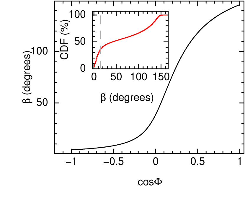
Figure 6: Main plot: Misalignment angle between the disc and BH spin axes, $\beta$, plotted against the cosine of the azimuthal viewing angle (see the text for details). This assumes our best fitting value for the disc inclination angle $i$ and a best fitting value of the BH spin inclination angle $\theta$ from the literature. Inset: Cumulative distribution function for $\beta$ which takes statistical measurement errors of $i$ and $\theta$ into account and assumes equal probability of measuring a given $\cos\Phi$.

In the precession model, the inner flow spin axis is assumed to precess around the BH spin axis, such that the angle between the BH and flow spin axes stays constant. Since Lense-Thirring precession does not occur in the BH equatorial plane, a misalignment between the disc and the BH spin axes is assumed. This way, the inner flow is being fed by a misaligned disc, driving precession. Defining the angle between the disc and BH axes as $\beta$, the angle between the BH and flow axes is also $\beta$ and the angle between the inner flow and the disc varies over a precession cycle from a minimum of $0$ to a maximum of $2\beta$ (see schematics in Veledina, Poutanen & Ingram 2013 and Ingram et al. 2015). This misalignment introduces a level of asymmetry not captured by our simple parameterisation of the disc illumination profile, since in our parameterisation the disc illumination profile is asymmetric throughout the precession cycle. For a misaligned system, in contrast, the illumination profile will be maximally asymmetric when the flow and disc are maximally misaligned, and will be axisymmetric when the flow and disc align. In other words, $A_{1}$ and $A_{2}$ would depend on QPO phase, becoming zero once per precession cycle, rather than remaining constant as we assume here. Nonetheless, it is clearly sensible to fit using the simplest possible model before introducing further complexity.

If the angle between the disc and flow is indeed changing during a precession cycle, this will drive changes in the reflection fraction. This is what we see in Fig. 5 with $3.5\sigma$ significance. In any case, this is indicative of systematic changes of the accretion geometry during a QPO cycle and provides yet more confirmation of the geometric origin of Type C QPOs. In the precession model, this implies that the flow aligns with the disc at a QPO phase of $\sim 0.25$ cycles when the reflection fraction dips.

In order to reproduce the observed QPO amplitude, the precession model requires $\beta\sim 10-15^{\circ}$ (Veledina et al. 2013; Ingram et al. 2015). Since here we measure the angle between our line-of-sight and the disc spin axis, $i$, and Steiner et al. (2012) used proper motion of the jet lobes to measure the angle between our line-of-sight and the jet, $\theta$, we can place some constraints on the misalignment angle $\beta$ (assuming the jet can be used as a proxy for the BH spin axis). Even if we know $i$ and $\theta$ to perfect precession, there is some unknown azimuthal angle, $\Phi$. Defining $\Phi$ on the disc plane following Ingram et al. (2015) and Veledina, Poutanen & Ingram (2013), the angles $\theta$ and $i$ are related as

$$\cos\theta=\sin i\sin\beta\cos\Phi+\cos i\cos\beta.$$ (8)

This is equation 3 in Ingram et al. (2015) and can be most easily derived using the coordinate system of Veledina, Poutanen & Ingram (2013) (see their Fig. 2). In their formalism, $\theta$ is the angle between the vectors $\mathbf{\hat{J}_{BH}}$ and $\mathbf{\hat{o}}$. We solve the above equation for $\beta$ assuming best fitting values of $i=70.68^{\circ}$ and $\theta=75^{\circ}$, running through the full range of viewer azimuth $\Phi$ (which is completely unknown). The result is plotted in the main panel of Fig. 6 (black line). We see that nearly the full range of possible $\beta$ values are allowed. Note that $\beta=0$ corresponds to alignment between the disc and BH spin, and $\beta=180^{\circ}$ corresponds to counter-alignment (see King et al. 2005 for a discussion on counter-alignment). We can take this further by simulating Gaussian distributed random variables for $i$ and $\theta$, and a uniformly distributed random variable for $\cos\Phi$. Since the measurement error on both $i$ and $\theta$ is $\sim 3^{\circ}$, we use this as the standard deviation for both of the Gaussian distributions. The inset plot in Fig. 6 shows the resulting cumulative probability distribution function for $\beta$. The grey dashed line shows $\beta=15^{\circ}$ which is consistent with our measurements within $0.5\sigma$ (the probability distribution peaks at $\sim 4^{\circ}$).

6.4 Continuum flux

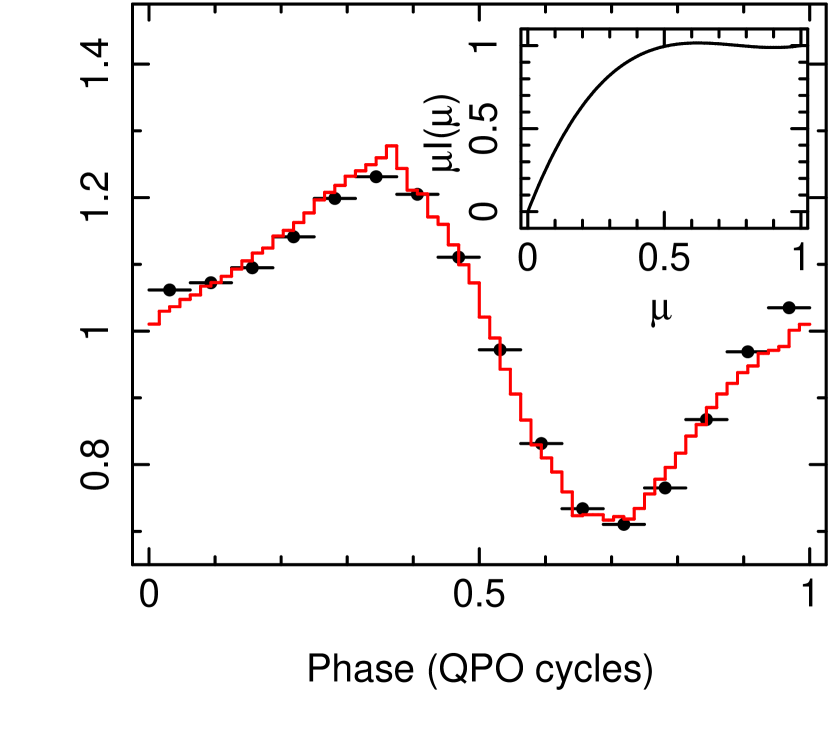
Figure 7: QPO waveform for orbit 2a (black points) and for the precession model (red line). The observed waveform is calculated in units of counts $s^{-1}$ and then divided by the mean count rate. The waveform calculation uses the limb darkening law shown in the inset ($\mu$ is the cosine of the instantaneous viewing angle). See the text for more details.

Our tomographic modeling indicates that the front and back of the disc are preferentially illuminated by the inner flow at QPO phases $\sim 0.4$ and $\sim 0.9$ cycles. As discussed in the previous sub-section, we also have measurements of the angles $\theta$ and $i$ and a measurement of the disc inner radius (=flow outer radius). The bottom panel of Fig. 5 indicates that the X-ray flux peaks at $\sim 0.35$ cycles. So can the precession model reproduce this waveform in a manner consistent with these constraints? Precession of the inner flow will modulate the X-ray continuum flux in (at least) three ways: 1) limb darkening, 2) changes in solid angle and 3) changes in Doppler boosting. The limb darkening law depends on the radiative process, which is Comptonization for the inner flow. For a stationary slab of Comptonizing material, the observed intensity of X-ray radiation depends on viewing angle, since photons that have undergone many scatterings are more likely to escape at a large inclination angle (e.g. Sunyaev & Titarchuk 1985; Viironen & Poutanen 2004). The more face-on we view the flow, the greater the solid angle. Without relativistic effects, the observed flux is simply the intensity $\times$ the solid angle. Doppler boosting has the opposite effect: the emission is maximally boosted when the flow is viewed maximally edge-on, since this maximizes the line-of-sight velocities. The observed flux as a function of precession angle is then a balance between these three considerations. Doppler boosting is most important at small radii due to the higher rotational velocity, and solid angle effects are most important for large radii since light bending tends to wash out solid angle variations close to the BH (Ingram et al. 2015; Veledina, Poutanen & Ingram 2013).

Since our definition of QPO phase $\gamma$ is fairly arbitrary, we must define a further parameter to tie $\gamma$ to the geometry. We define the QPO phase such that angle between our line-of-sight and the flow spin axis is at a minimum when $\gamma=\gamma_{0}$. In other words, the flow spin axis comes the closest to pointing at the observer when $\gamma=\gamma_{0}$, corresponding to a maximum in the observed solid angle. We use the code described in Ingram et al. (2015) to calculate the flux as a function of $\gamma$ (i.e. the QPO waveform), fixing $i=70.68^{\circ}$, $\theta=75^{\circ}$ and flow outer radius $=31.47~{}R_{g}$. We leave $\gamma_{0}$ as a free parameter, in order to compare the model waveform with the observed waveform. The value of $\gamma_{0}$ that best reproduces the observed waveform therefore tells about when in the QPO cycle the flow spin axis is predicted to be maximally facing us. The code takes all relativistic effects into account, and also includes obscuration of the flow by the disc. We take the flow to be a torus with scale height $h/r=0.1$ (see Ingram et al. 2015 for details of the flow geometry). We parameterise the limb darkening law as

$$I(\mu)\propto b_{0}-I_{0}+b_{1}\mu+b_{2}\mu^{2}.$$ (9)

Here, $\mu$ is the cosine of the angle between the observer’s line-of-sight and the flow spin axis, and $I_{0}$ is set to ensure that the minimum of $I(\mu)$ in the range $\mu=0-1$ is $I_{min}=b_{0}$. In Ingram et al. (2015) $b_{0}$, $b_{1}$ and $b_{2}$ were set to reproduce the Compton scattering limb darkening law for optical depth $\tau=1$ derived by Sunyaev & Titarchuk (1985). Here, we leave them as free parameters. We also leave the misalignment angle $\beta$ as a free parameter. The remaining parameter is the inner radius of the flow, or at least the inner radius at which the flow radiates.

We compare our waveform model to the $4-10$ keV QPO waveform of XMM-Newton orbit 2a, derived using the method of IK15 (Fig 7). We perform a least-squared fit, but note that correlated errors between the QPO phases mean that $\chi^{2}$ does not give a reliable indication of goodness of fit (see Section 2.2). We simply use this fitting as an exercise to try and roughly match the data. For our ‘best fit’ model, we set $b_{0}\approx 0.3$, $b_{1}\approx-1.75$ and $b_{2}\approx 0.76$, which gives the limb darkening law shown in the inset of Fig. 7. This roughly matches the limb darkening law expected for Compton scattering with an optical depth $\tau\approx 0.5$ (see Fig. 7a of Sunyaev & Titarchuk 1985). We set the inner flow radius to $11~{}R_{g}$. This is fairly large, being outside of the ISCO even for a maximally retrograde BH, but we find that the amplitude of the waveform is sensitive to the difference between flow outer and inner radii. This is because of the balance between Doppler boosting and solid angle effects: the flux from a very small radius is out of phase with the flux from a very large radius, since the former is dominated by Doppler boosting and the latter is dominated by solid angle variations. The amplitude of the waveform is therefore damped by destructive interference between different radii. It is not unreasonable for a misaligned flow to have a fairly large inner radius, since it has been shown in General Relativistic magneto hydrodynamic simulations that torques from the frame dragging effect can create plunging streams at the so-called bending wave radius, truncating the flow outside of the ISCO (Fragile et al. 2007; Ingram, Done & Fragile 2009; Fragile 2009). The ‘best fit’ misalignment angle is $\beta\approx 11^{\circ}$, which is compatible with the measurements presented in the previous sub-section.

Finally, we find a ‘best fit’ value of $\gamma_{0}\approx 0.17$ cycles. This means that the flow spin axis maximally faces us at a QPO phase of $\gamma=0.17$ cycles, and maximally faces away from us at $\gamma=\gamma_{0}+0.5=0.67$ cycles. From Fig. 5, we see that this roughly corresponds with the two maxima in line energy. Therefore, combining tomographic modelling with the waveform modelling implies that the flow appears to the observer to shine preferentially on the left and right of the disc when it is maximally facing us. This is the opposite to what I16 suggested. There, the suggestion was that the front and back of the flow illuminate the disc such that, when the flow is facing us, it illuminates the front and back of the disc as we see it. Whether or not this is credible should be tested with more sophisticated calculations. For the values we used for $\beta$, $i$ and $\theta$, it can be derived from equation 8 that $\Phi\approx 110^{\circ}$. Further taking into account the fitted value of $\gamma_{0}$, indicates that the flow aligns with the disc at a QPO phase of $\gamma\approx 0.35$ cycles. The QPO phase with the lowest observed reflection fraction gives an independant estimate for the alignment phase. We see in Fig. 5 that the minimum in reflection fraction occurs at $\gamma\sim 0.25$ cycles, which disagrees somewhat with the $\sim 0.35$ cycles derived from waveform fitting.

Nonetheless, it is encouraging that we can achieve a reasonable match to the observed QPO waveform, given the relative simplicity of both our tomographic and waveform models. A modulation mechanism our waveform model does not take into account is variation of seed photons. As the misalignment angle between the disc and flow changes over a precession cycle, the flow sees a varying luminosity of disc photons. This will introduce a modulation into the intrinsic luminosity of the flow (Życki, Done & Ingram in prep). This oscillation of the misalignment angle will also drive spectral pivoting as the disc cooling changes, in addition to the aforementioned changes in reflection fraction. We do observe a modulation in $\Gamma$ for our best fit tomographic model (see Fig. 5), but this is not statistically significant. It is also likely that the optical depth, and therefore the limb darkening law, is a function of radius (Axelsson et al. 2014), which will complicate the picture further. It is very hard to see how alternative mechanisms for the iron line centroid modulation, such as oscillations in the disc inner radius, ionisation parameter or radial emissivity, can be compatible with the observed QPO waveform.

We calculate the Lense-Thirring precession frequency for a flow with a flat surface density profile extending from $11~{}R_{g}$ to $31.67~{}R_{g}$ (see equation 1 in Ingram & Done 2012a, where $f_{LT}$ is given in equation 3 of Ingram & Motta 2014), and our BH spin value of $a=0.21$. The mass of H 1743–322 is unknown, but the mass distribution function for Galactic BHs peaks at $\sim 6.3M_{\odot}$ (Özel et al. 2010; Farr et al. 2011). Using this value for mass gives a precession frequency of $0.25$ Hz, which matches the observed QPO frequency well. If we instead use $M=9.3M_{\odot}$, consistent with the estimate of $M\gtrsim 9.29M_{\odot}$ obtained by Ingram & Motta (2014) using high frequency QPOs, the precession frequency becomes $0.17$ Hz.

6.5 Biases in the time-averaged line profile

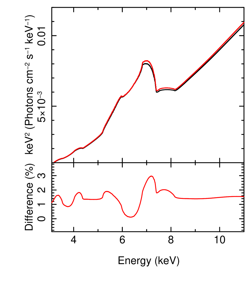
Figure 8: Top: Phase-averaged reflection spectrum, zoomed in on the iron line, for our best fit model (black) and also calculated by setting all the parameters to their phase-averaged values (red). A small bias is created by non-linear variability. Bottom: The percentage difference between the two spectra (red line minus the black line, then divided by the black line and multiplied by $100\%$). We see an approximately constant $\sim 1\%$ offset, with features around the iron line on the $\sim 2\%$ level.

For our best fitting model, the spectrum is varying with QPO phase in a non-linear fashion. This means that the phase-averaged spectrum is not exactly equal to a spectrum computed using the phase-averaged parameter values. Since time-averaged spectral modelling implicitly makes the assumption that the affects of non-linear spectral variability are negligible, this may lead to biases. In order to investigate these biases, we can first compare our fits to the time-averaged spectrum in Section 1 with our best fitting tomographic model (see Tables 1 and 2). We see that the tomographic modelling yields a slightly smaller truncation radius and a slightly higher inclination, although they are consistent within errors. The fact that these sets of parameters are consistent with one another implies that biases due to non-linear spectral variability (which are automatically accounted for in our tomographic modelling but ignored for the time-averaged spectral fits), are small.

In Fig. 8, we assess the importance of non-linear affects more directly. The black line shows the phase-averaged reflection spectrum corresponding to our best-fit parameters. Here, we have calculated the spectrum for the full range of QPO phases, and taken the mean. For the red line, we take our best fitting model, set $A_{1}=A_{2}=0$, $\Gamma(\gamma)=\Gamma_{0}$, $f(\gamma)=f_{0}$ (therefore removing all non-linear variability) and calculate the phase-averaged spectrum. We see that this slightly over-predicts the size of the blue horn, but is a $\sim 2\%$ effect (see bottom panel). Therefore, we conclude that the bias is small and likely does not introduce significant systematic errors into time-averaged spectral fits, at least for these data. We do stress, however, that considering variability properties in addition to the time-averaged spectrum is always advantageous since it uses more information.

6.6 Assumptions

We have developed the first physical model for QPO phase-resolved spectroscopy. There are a number of improvements that could be made to our physical assumptions in future. The model we use for the reflection continuum, $xillver$, is the current state-of-the-art, but improvements are still being made. First of all, $xillver$ models the illuminating continuum as an exponentially cut-off power-law, whereas a sharper high energy cut-off is associated with thermal Compton up-scattering (Zdziarski, Johnson & Magdziarz 1996; Fabian et al. 2015). Also, the disc is assumed to be a constant density slab. Making the more physical assumption of hydrostatic equilibrium affects the predicted reflection spectrum, but less so in the $>4$ keV range we consider (Nayakshin, Kazanas & Kallman 2000; Done & Nayakshin 2007). For this paper, we simply parameterise the radial dependence of the irradiating flux as $r^{-3}$. This will be true far from the BH, but not close to the irradiating source (e.g. Laor 1991; Wilkins & Fabian 2012). We have also made the simplifying assumption that the rest-frame reflection spectrum is the same for the whole disc, allowing us to convolve the rest-frame spectrum with a smearing kernel. However, in reality the ionisation parameter will depend on radius since disc irradiation depends strongly on proximity to the continuum source. Svoboda et al. (2012) showed that not accounting for this can lead to measurement of very centrally peaked emissivity profiles ($\sim r^{-7}$), as is often the case (e.g. Wilkins & Fabian 2011; Fabian et al. 2012). Also, light bending means that different parts of the disc have different observed inclination angles, which makes a difference to the spectrum because of the limb darkening law of reflected emission (Svoboda et al. 2009; García et al. 2014). Finally, our assumed azimuthal emissivity profile is rather simplistic, but this allows us to define a generic model to compare with the data. This can be calibrated against more involved theoretical modeling in future.

7 Conclusions

We have developed the first physical model for QPO phase-resolved spectroscopy and fit it to data from the BH binary system H 1743–322. We find that the reflection fraction varies systematically with QPO phase ($3.52\sigma$), adding to the now formidable body of evidence in favour of a geometric origin of Type C QPOs. Our model mimics the asymmetric illumination pattern, rotating about the disc surface, that would be produced by a precessing inner flow with a simple analytic parameterisation. It provides a good description of the observed shifts in the iron line energy and is preferred over a null-hypothesis of axisymmetric illumination with $2.40\sigma$ significance. More data is therefore needed if a direct $3\sigma$ detection of asymmetric disc illumination is to be achieved. We consider alternative axisymmetric models, but none of them adequately describe the data. Our results, alongside the results of I16, provide strong evidence that Type C QPOs are driven by precession. We note that precession of the disc rather than the flow is also possible. We expand upon our results by modelling the continuum flux as a function of QPO phase with a precessing inner flow model (Fig. 7), and find we can match the observed QPO waveform for a specific geometry in which the flow spin axis faces us at a QPO phase of $\sim 0.2$ cycles. Since this roughly coincides with a maximum in iron line centroid energy, this implies that the flow preferentially illuminates the left and right hand sides of the disc when it maximally faces us. This geometry can be tested with direct modelling of the illumination profile from a precessing flow in future, together with more sophisticated continuum flux waveform modelling. Tomographic modelling of QPOs is a powerful new technique. The next step is to apply the technique to more data in order to track changes in accretion geometry of a source throughout an outburst.

References

- Axelsson et al. (2014) Axelsson M., Done C., Hjalmarsdotter L., 2014, MNRAS, 438, 657
- Bardeen & Petterson (1975) Bardeen J. M., Petterson J. A., 1975, ApJ, 195, L65
- Blandford & Znajek (1977) Blandford R. D., Znajek R. L., 1977, MNRAS, 179, 433
- Cabanac et al. (2010) Cabanac C., Henri G., Petrucci P.-O., Malzac J., Ferreira J., Belloni T. M., 2010, MNRAS, 404, 738
- Casella et al. (2005) Casella P., Belloni T., Stella L., 2005, ApJ, 629, 403
- De Marco & Ponti (2016) De Marco B., Ponti G., 2016, ArXiv e-prints
- Dexter & Agol (2009) Dexter J., Agol E., 2009, ApJ, 696, 1616
- Done (2010) Done C., 2010, ArXiv e-prints
- Done et al. (2007) Done C., Gierlinski M., Kubota A., 2007, A&A, 15, 1
- Done & Nayakshin (2007) Done C., Nayakshin S., 2007, MNRAS, 377, L59
- Fabian et al. (2015) Fabian A. C., Lohfink A., Kara E., Parker M. L., Vasudevan R., Reynolds C. S., 2015, MNRAS, 451, 4375
- Fabian et al. (1989) Fabian A. C., Rees M. J., Stella L., White N. E., 1989, MNRAS, 238, 729
- Fabian et al. (2012) Fabian A. C., Wilkins D. R., Miller J. M., Reis R. C., Reynolds C. S., Cackett E. M., Nowak M. A., Pooley G. G., Pottschmidt K., Sanders J. S., Ross R. R., Wilms J., 2012, MNRAS, 424, 217
- Farr et al. (2011) Farr W. M., Sravan N., Cantrell A., Kreidberg L., Bailyn C. D., Mandel I., Kalogera V., 2011, ApJ, 741, 103
- Fragile (2009) Fragile P. C., 2009, ApJ, 706, L246
- Fragile et al. (2007) Fragile P. C., Blaes O. M., Anninos P., Salmonson J. D., 2007, ApJ, 668, 417
- Galeev et al. (1979) Galeev A. A., Rosner R., Vaiana G. S., 1979, ApJ, 229, 318
- García et al. (2014) García J., Dauser T., Lohfink A., Kallman T. R., Steiner J. F., McClintock J. E., Brenneman L., Wilms J., Eikmann W., Reynolds C. S., Tombesi F., 2014, ApJ, 782, 76
- García et al. (2013) García J., Dauser T., Reynolds C. S., Kallman T. R., McClintock J. E., Wilms J., Eikmann W., 2013, ApJ, 768, 146
- Gierliński et al. (2002) Gierliński M., Done C., Barret D., 2002, MNRAS, 331, 141
- Haardt & Maraschi (1991) Haardt F., Maraschi L., 1991, ApJ, 380, L51
- Heil et al. (2015) Heil L. M., Uttley P., Klein-Wolt M., 2015, MNRAS, 448, 3348
- Homan et al. (2005) Homan J., Miller J. M., Wijnands R., van der Klis M., Belloni T., Steeghs D., Lewin W. H. G., 2005, ApJ, 623, 383
- Ichimaru (1977) Ichimaru S., 1977, ApJ, 214, 840
- Ingram & Done (2012a) Ingram A., Done C., 2012a, MNRAS, 419, 2369
- Ingram & Done (2012b) Ingram A., Done C., 2012b, MNRAS, 427, 934
- Ingram et al. (2009) Ingram A., Done C., Fragile P. C., 2009, MNRAS, 397, L101
- Ingram et al. (2015) Ingram A., Maccarone T. J., Poutanen J., Krawczynski H., 2015, ApJ, 807, 53
- Ingram & Motta (2014) Ingram A., Motta S., 2014, MNRAS, 444, 2065
- Ingram & van der Klis (2015) Ingram A., van der Klis M., 2015, MNRAS, 446, 3516
- Ingram et al. (2016) Ingram A., van der Klis M., Middleton M., Done C., Altamirano D., Heil L., Uttley P., Axelsson M., 2016, MNRAS, 461, 1967
- King et al. (2005) King A. R., Lubow S. H., Ogilvie G. I., Pringle J. E., 2005, MNRAS, 363, 49
- Kolehmainen et al. (2014) Kolehmainen M., Done C., Díaz Trigo M., 2014, MNRAS, 437, 316
- Laor (1991) Laor A., 1991, ApJ, 376, 90
- Lense & Thirring (1918) Lense J., Thirring H., 1918, Physikalische Zeitschrift, 19, 156
- Luminet (1979) Luminet J.-P., 1979, A&A, 75, 228
- Markoff et al. (2005) Markoff S., Nowak M. A., Wilms J., 2005, ApJ, 635, 1203
- Matt et al. (1993) Matt G., Fabian A. C., Ross R. R., 1993, MNRAS, 262, 179
- Middleton & Ingram (2015) Middleton M. J., Ingram A. R., 2015, MNRAS, 446, 1312
- Miller & Homan (2005) Miller J. M., Homan J., 2005, ApJ, 618, L107
- Motta et al. (2015) Motta S. E., Casella P., Henze M., Muñoz-Darias T., Sanna A., Fender R., Belloni T., 2015, MNRAS, 447, 2059
- Nayakshin et al. (2000) Nayakshin S., Kazanas D., Kallman T. R., 2000, ApJ, 537, 833
- Novikov & Thorne (1973) Novikov I. D., Thorne K. S., 1973, in Dewitt C., Dewitt B. S., eds, Black Holes (Les Astres Occlus) Astrophysics of black holes.. Gordon and Breach, New York, pp 343–450
- Özel et al. (2010) Özel F., Psaltis D., Narayan R., McClintock J. E., 2010, ApJ, 725, 1918
- Plant et al. (2015) Plant D. S., Fender R. P., Ponti G., Muñoz-Darias T., Coriat M., 2015, A&A, 573, A120
- Ross & Fabian (2005) Ross R. R., Fabian A. C., 2005, MNRAS, 358, 211
- Schnittman et al. (2006) Schnittman J. D., Homan J., Miller J. M., 2006, ApJ, 642, 420
- Shakura & Sunyaev (1973) Shakura N. I., Sunyaev R. A., 1973, A&A, 24, 337
- Shaposhnikov & Titarchuk (2009) Shaposhnikov N., Titarchuk L., 2009, ApJ, 699, 453
- Sobolewska & Życki (2006) Sobolewska M. A., Życki P. T., 2006, MNRAS, 370, 405
- Steiner et al. (2012) Steiner J. F., Reis R. C., Fabian A. C., Remillard R. A., McClintock J. E., Gou L., Cooke R., Brenneman L. W., Sanders J. S., 2012, MNRAS, 427, 2552
- Stella & Vietri (1998) Stella L., Vietri M., 1998, ApJ, 492, L59+
- Stevens & Uttley (2016) Stevens A. L., Uttley P., 2016, ArXiv e-prints
- Stiele & Yu (2016) Stiele H., Yu W., 2016, ArXiv e-prints
- Sunyaev & Titarchuk (1985) Sunyaev R. A., Titarchuk L. G., 1985, A&A, 143, 374
- Sunyaev & Truemper (1979) Sunyaev R. A., Truemper J., 1979, Nature, 279, 506
- Svoboda et al. (2009) Svoboda J., Dovčiak M., Goosmann R., Karas V., 2009, A&A, 507, 1
- Svoboda et al. (2012) Svoboda J., Dovčiak M., Goosmann R. W., Jethwa P., Karas V., Miniutti G., Guainazzi M., 2012, A&A, 545, A106
- Tagger & Pellat (1999) Tagger M., Pellat R., 1999, A&A, 349, 1003
- Thorne & Price (1975) Thorne K. S., Price R. H., 1975, ApJ, 195, L101
- Uttley et al. (2014) Uttley P., Cackett E. M., Fabian A. C., Kara E., Wilkins D. R., 2014, Astronomy and Astrophysics Reviews, 22, 72
- van den Eijnden et al. (2016) van den Eijnden J., Ingram A., Uttley P., 2016, ArXiv e-prints
- van der Klis et al. (1987) van der Klis M., Hasinger G., Stella L., Langmeier A., van Paradijs J., Lewin W. H. G., 1987, ApJ, 319, L13
- Veledina et al. (2013) Veledina A., Poutanen J., Ingram A., 2013, ApJ, 778, 165
- Viironen & Poutanen (2004) Viironen K., Poutanen J., 2004, A&A, 426, 985
- Wagoner et al. (2001) Wagoner R. V., Silbergleit A. S., Ortega-Rodríguez M., 2001, ApJ, 559, L25
- Wijnands et al. (1999) Wijnands R., Homan J., van der Klis M., 1999, ApJ, 526, L33
- Wilkins & Fabian (2011) Wilkins D. R., Fabian A. C., 2011, MNRAS, 414, 1269
- Wilkins & Fabian (2012) Wilkins D. R., Fabian A. C., 2012, MNRAS, 424, 1284
- Wilkinson et al. (2011) Wilkinson T., Patruno A., Watts A., Uttley P., 2011, MNRAS, 410, 1513
- Wilms et al. (2000) Wilms J., Allen A., McCray R., 2000, ApJ, 542, 914
- Zdziarski et al. (1996) Zdziarski A. A., Johnson W. N., Magdziarz P., 1996, MNRAS, 283, 193