Adaptive Neuron Apoptosis for Accelerating Deep Learning on Large Scale Systems

Abstract

We present novel techniques to accelerate the convergence of Deep Learning algorithms by conducting low overhead removal of redundant neurons – apoptosis of neurons – which do not contribute to model learning, during the training phase itself. We provide in-depth theoretical underpinnings of our heuristics (bounding accuracy loss and handling apoptosis of several neuron types), and present the methods to conduct adaptive neuron apoptosis. Specifically, we are able to improve the training time for several datasets by 2-3x, while reducing the number of parameters by up to 30x (4-5x on average) on datasets such as ImageNet classification. For the Higgs Boson dataset, our implementation improves the accuracy (measured by Area Under Curve (AUC)) for classification from 0.88/1 to 0.94/1, while reducing the number of parameters by 3x in comparison to existing literature. The proposed methods achieve a 2.44x speedup in comparison to the default (no apoptosis) algorithm.

I Introduction

Deep Learning algorithms emulate computation structure of a brain by learning models using neurons and their interconnections (synapses, also known as parameters/weights) [1]. Using a cascade of neurons, Deep Learning algorithms are known to learn complex non-linear functions. These functions can be applied to both supervised (input dataset with ground truth labels) and unsupervised (input data with no labels) problems. Naturally, Deep Learning algorithms are being applied to several domains including Computer Vision [2], Speech Recognition [3], and High Energy Physics [4].

An important aspect of Deep Learning algorithms is the topology of a Neural Network (used interchangeably with Deep Learning with rest of the paper). A candidate topology may have a single input and an output layer, with possibly several hidden layers. Convolutional Neural Networks (CNN) – a class of Deep Learning algorithms – may have several convolutional layers, followed by several fully-connected layers. In practice, the neurons and synapses are implemented by using matrices, where each row/column represents a neuron and each element represents the strength (weight) of a synapse. The output of a neural network is the weight matrices, which may be used for Machine Learning tasks such as classification, or clustering.

Usually, a neural network topology is user-specified, which includes the number of hidden layers and number of neurons in each layer (an example is shown in Figure 1 (a)). Deeper neural networks (with more layers) are used for model generation from increasingly complex datasets, possibly learning complex non-linear functions. Bigger networks – which have larger number of neurons per layer – may also be used in addition to deeper networks for this purpose.

However, deeper and/or bigger networks do not necessarily provide better models. With increasing number of network parameters (the overall number of synapses), the training time per epoch increases significantly [5, 6]. Deeper networks tend to suffer from problems such as vanishing gradients [7], where the weights of network parameters change slowly. In addition, deeper networks are known to cause overfitting – a scenario in which the model has learned very well from the training set, but does not generalize well on new samples. This scenario generally occurs when a neural network has learned a significantly more complex function than implied by the training set. A few possible solutions such as Dropout [8] exist – but they do not reduce the overall time to solution. Lastly, larger number of parameters have prohibitive storage and computational requirements during the testing phase (when the model is applied on new data) – which is problematic for deployment on power/memory constrained devices.

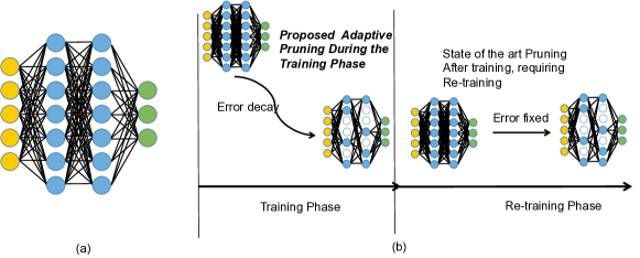
Figure 1: (a) An example of a Deep Neural Network (DNN) with two hidden layers (color coded - blue) (b) Comparison of our approach (adaptive apoptosis during the training phase) to state of the art approaches, which conduct removal of non-contributing synapses after training is over. Unlike state of the art approaches, the proposed approach does not require re-training

A possible solution to this problem is to prune the neural network. Usually, this is conducted after the training is completed by removing unnecessary weights (and possibly) neurons [9, 10, 11]. After pruning, the network is re-trained to stabilize the parameters [10] (The scenario is shown on the right of Figure 1(b)). Usually pruning implies that unnecessary parameters (and in a few cases neurons) may be removed, without accuracy loss.

However, there are several shortcomings of existing approaches: 1) Re-training is a time-consuming process. As an example, Han et al. report a slowdown of up to 2.5x when re-training after pruning [10]. This is especially problematic for large datasets, where increasing the training time is unattractive. 2) Another problem with the current approaches is the lack of theoretical underpinnings for network pruning. Usually, this is not required for state of the art networks, because they use the final network as starting point for re-training. After each sub-step of pruning and re-training, the accuracy is compared against the reference network – to ensure no empirical loss of accuracy. However, this approach is not always efficient, since this exploration is is expensive in time due to several re-training steps.

Our objective in this paper is to remove unnecessary neurons (and hence synapses) for Deep Learning algorithms by adaptively removing redundant neurons – neuron apoptosis – during the training phase itself, while achieving similar accuracy as achieved without apoptosis using the original neural network. Unlike existing approaches, our adaptive apoptosis approach reduces the overall training time – which makes it a very attractive solution for reducing the computational/storage requirements, while gaining speedup during the training phase itself.

I-A Contributions:

Specifically, we make the following contributions in this paper:

• We propose novel heuristics to adaptively conduct neuron apoptosis during the training phase. We provide an in-depth discussion of the point of initial apoptosis, subsequent apoptosis and degree of apoptosis. Our heuristics rely on the intuition of the basic structure of the loss function (independent of the dataset), in addition to heuristics, which consider linear apoptosis.

• We provide theoretical underpinnings of our proposed solution. These are intended to bound the loss of accuracy incurred by neuron apoptosis and address challenges of considering input/output synapses to neuron types for apoptosis. Unlike existing literature – where neuron pruning is executed after training to prevent accuracy loss – this is a critical step to ensure the correctness of proposed heuristics.

• We extend Caffe to use MPI (similar to FireCaffe [12]) – so that the execution may be conducted on supercomputers, and other large scale systems (such as cloud computing systems). With these extensions, our implementations is able to utilize large scale clusters using native implementations with multi-core systems and accelerators such as GPUs.

• We evaluate our proposed implementations with two clusters – one connected with Intel Haswell and InfiniBand, and other connected with nVIDIA GPUs and InfiniBand. We use several large datasets for evaluation using multiple nodes on each cluster. Our evaluation indicates a reduction of up to 30x in overall parameters, a speedup of 2-3x – unlike existing approaches which cause slowdown.

A very important science contribution of our paper is the improvement in classification accuracy of Higgs Boson Dataset (represented by Receiver Operating Curve (ROC) - Area Under Curve (AUC)) published in the literature by Sadowski et al. [4]. We are able to improve the AUC by 6 percentage points (from 0.88/1 to 0.94/1), while reducing the number of parameters by 3x and obtaining a speedup of 2.44x in comparison to the default (no apoptosis) algorithm. Another important artifact of our approach is the reduction in space and computational requirements of the neural networks (up to 30x), which can be realized without incurring a penalty in training time.

The rest of the paper is organized as follows: In section II, we present related work on neural network topologies. In section III, we provide a brief introduction to neural networks and Google TensorFlow. In section IV, we present a solution space to the problem of neuron apoptosis, possible design choices, heuristics and perceived benefits. We also present theoretical underpinnings of our proposed solutions (section V), and provide a proof on bounds to accuracy loss. We present detailed performance evaluation in section VII and present conclusions in section VIII.

II Related Work

We split the related work section on Deep Learning algorithms and implementations in research on large scale systems and pruning/compression algorithms.

II-A Systems (Multi-core/Many-core/Large Scale) Research

The most widely used algorithm for training Deep Learning algorithms is batch gradient descent. Several implementations of batch gradient descent methods are available for sequential, multi-core and many-core systems such as GPUs. The most prominent implementations are Caffe [13] (GPUs), Warp-CTC (GPUs), Theano [14, 15] (CPUs/GPUs), Torch [16] (CPUs/GPUs), and Google TensorFlow [17] which uses nVIDIA CUDA Deep Neural Network (cuDNN) and a multi-threaded implementation of batch gradient descent methods.

Caffe has emerged as one of the leading Deep Learning software, which can be used for developing novel extensions, such as ones proposed in this paper. Caffe supports execution on single node (connected with several GPUs) and recent extensions include support on Intel systems. While we conduct the proposed research with Caffe, the proposed extensions can also be applied with TensorFlow.

Classical neural networks were shallow (1-2 layers), where batch gradient descent methods worked well. However, with deeper networks, the algorithms frequently suffered from the vanishing gradient problem [18]). The standard algorithm for training them (described in section III) fails because the gradients become smaller by several orders of magnitude as the network becomes deeper. This problem was solved in [19] and [20], who demonstrated that a network can be trained one layer at a time with autoencoders [21], and then put it together into a single network for classification [22]. Another solution, that we will use, are rectified linear units, which have become the standard in the field, though our results are valid for other types of neurons as well. These optimizations are available in Caffe and other Deep Learning packages.

II-B Neural Network Pruning/Compression

Network pruning is typically considered for reducing the memory and computational requirements for execution on embedded devices. Compression algorithms are then applied on these pruned networks for realizing further memory savings.

In biology, apoptosis – the death of neurons – and its inverse neurogenesis, have been studied [23], and it has been determined that these processes can aid in learning effectively. Chambers et al. modeled the apoptosis/neurogenesis process by re-initializing the weights of randomly selected neurons periodically. Their study concluded that periodic apoptosis can improve the performance of a network. This forms the basis of our paper – by conducting adaptive apoptosis during the training phase.

Several researchers have conducted offline neuron apoptosis – after the completion of the training phase. This is in sharp contrast to our proposed approach, in which apoptosis is conducted during the training phase itself, which reduces the overall training time, while reducing the space requirements. For offline apoptosis, researchers have conducted neuron apoptosis due to a lack of computational resources [24], regularization to prevent overfitting [25], which provides algorithms for removing synapses and possibly neurons. Kamruzzman et al. have demonstrated similar results [26], where the fundamental objective is to remove redundant weights, and possibly neurons. The pruning has been also applied for generating human-usable rules for classification [27]. Other researchers have considered temporary neuron pruning – typically referred as Dropout, proposed by Hinton et al.  [28]. A selective Dropout is proposed by other authors [29]. However, since the Dropout is temporary, they do not affect the final topology of the neural network – although they help with regularization.

Recently, Han et al. have proposed methods to remove non-contributing weights after the training phase [10]. However, this incurs significant slowdown (up to 2.5x). Other approaches – such as HashedNets – compress the neural networks without removing weights/neurons [30]. Murray and Chiang have proposed methods to remove non-contributing synapses (which are significantly different from our approach of removing redundant neurons) [31, 32]. Since we are primarily focused on removing redundant neurons adaptively, we consider our approaches to be complimentary to their approach.

III Fundamentals

III-A Neural Networks

Neural Networks are a class of Machine Learning algorithms, which emulate the computational structure of the brain to learn nonlinear functions. The basic unit of a neural network is a neuron, and neurons are interconnected using synapses.

III-A1 Activation Functions

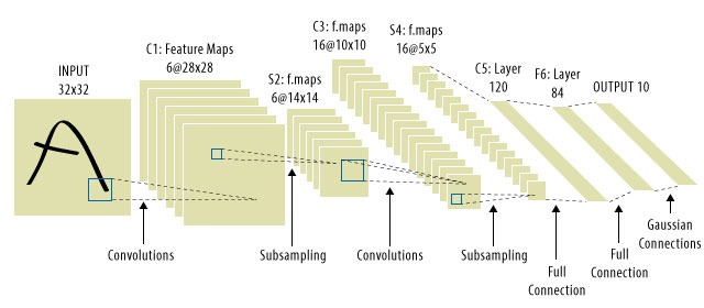
Figure 2: An example of CNN execution on letter “A” from MNIST with LeNet-5 [33]

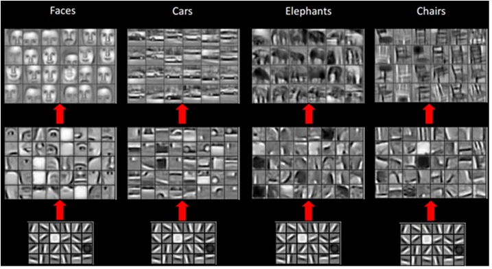
Figure 3: Pictorial representation of features in 3 layers of a CNN [34]. Notice the increasing complexity of features – although first level features are the same

There are several common nonlinear activation functions for neural networks. In this paper, we will specifically focus on the two most widely used, rectified linear units (ReLU) and sigmoid units.

$$\mathrm{sigmoid}(x) = \frac{1}{1+\exp(-x)}$$ (1)

$$\mathrm{ReLU}(x) = \max(0,x)$$ (2)

III-A2 Convolutional Neural Networks

Convolutional Neural Networks (CNN) are a widely used type of neural network, which are specifically designed to preserve structure in the data, such as the sequence of sounds in speech data or the relative positions of pixels and features in an image.

The fundamental unit of computation in CNN is a convolution – which are arrays in some dimension – unlike vectors in DNN. Each neuron in a convolution layer considers input from a small window (such as 3x3,5x5) in an image, applies a convolution and computes a value, which is an indirect representation of the confidence of the feature detected by the neuron. The window based computational structure is useful for structured datasets, which can use a cascade of convolutional layers to incrementally generate more complex features. An example of CNN is shown in Figure 3, and Figure 3 represents the features learned by a CNN using a cascade of convolution layers. Besides convolution layers, a neural network may also consist of pooling layers, which are also used for alleviating overfitting to the presence of a feature in an image.

III-B Caffe

Caffe [13] is a popular software package which provides abstractions for building neural networks of a wide range of topologies and training them with a wide range of optimizers. Caffe provides abstractions of operations on tensors (multi-dimensional arrays), which are used for implementing Deep Learning algorithms. Caffe builds a computational graph which consists of an input tensor followed by tensors for each individual hidden layer and output. We choose Caffe because it is heavily optimized, and can be modified effectively through both the C++ backend and a Python interface.

Caffe’s runtime is implemented using C++ – which makes it attractive for extracting native performance. We have modified this code for distributed memory implementation on large scale systems, using MPI to natively use network hardware and obtain optimal performance. This is similar to FireCaffe [35], another distributed memory implementation of Caffe. Additionally, Caffe abstracts GPU computations by leveraging nVIDIA CUDA Deep Neural Network Library (cuDNN). As a result, the implementations are able to use large scale systems on traditional multi-core systems and many-core systems connected with GPUs.

IV Neuron Apoptosis Solution Space

In this section, we present a solution space for neuron apoptosis. There are several important design considerations: the point of initial apoptosis, when to conduct the subsequent apoptosis, apoptosis termination and degree of apoptosis. We present design considerations for each of these topics.

IV-A Point of Initial Apoptosis

The intuition behind initial apoptosis comes from the mammalian brain. A significant apoptosis at any stage may have drastic consequences – especially one very early or late in life. However, the mammalian brain loses neurons periodically while retaining the fidelity of previously learned models (such as object, taste and voice recognition).

IV-A1 Quarter-Life

We take inspiration from particle physics to consider half-life to be the point of initial apoptosis. It is possible to calculate half-life statically (by using the number of epochs/training time provided by the user – generally as an input). However, with initial point as half-life, we would possibly be conducting apoptosis at end of life. Hence, we instead consider the point of initial apoptosis to be quarter-life.

IV-A2 Random

It is also possible to consider random time-stamp/epoch during training as the initial point of apoptosis. In most cases, if the initial apoptosis occurs early, it would lead to significant pruning with potentially significant damage to the model accuracy. In other cases (such as quarter-life/half-life/end of training), it would generate a high fidelity model, albeit without observing speedup in training time.

IV-A3 End of Training

Previously proposed approaches perform apoptosis at the end of training. These techniques remove synapses that fail to contribute, rather than redundant neurons. However, this approach requires a re-training phase, as in Han et al. [10]. To ensure that training time does not increase, we do not pursue this heuristic.

IV-B Subsequent Apoptosis

Another important design consideration is when to conduct subsequent apoptosis. We present intuition behind our design choices here:

IV-B1 Fixed/Random

An intuitive heuristic is to conduct subsequent apoptosis at fixed/random intervals. While there are several advantages to fixed/random apoptosis, a high frequency would result in many distance calculations, most of which will not result in any significant apoptosis (as the weights would not change dramatically). On the other hand, a low frequency would likely conduct less apoptosis of neurons, but would allow for a more significant change in weights when compared to a high frequency.

IV-B2 Logarithmic

We draw inspiration from the properties of loss functions in Deep Learning algorithms for making a case of logarithmic number of apoptoses. In general, the decay of the loss function can be well represented using an exponential decay function. Hence, it is expected that the subsequent apoptosis at logarithmic steps will handle half-life of errors. Additionally, with logarithmic number of apoptosis, the overall time spent in distance calculations would also be minimized.

IV-C Temporal Degree of Apoptosis

Another design consideration is the temporal degree of apoptosis. Essentially, it is important to consider whether apoptosis should remain fixed, become increasingly aggressive or conservative:

IV-C1 Fixed

The default choice is to use a fixed degree of apoptosis. The expectation with this approach is to ensure that rate of redundant neuron pruning is fixed over time.

IV-C2 Increasingly Aggressive

The intuition behind increasingly aggressive apoptosis is that the overall possibility to prune redundant neurons is diminished – as the termination criteria is reached. The rate at which degree increases itself has several choices (such as fixed-linear, random and others). For simplicity, we propose to increase the degree of apoptosis linearly – although without loss of generality, other functions may be applied as well.

IV-C3 Increasingly Conservative

On the contrary, the intuition behind conservative apoptosis is to save the remaining neurons (after initial apoptosis) as much as possible, especially if the early apoptosis already prunes the majority of redundant neurons. Without loss of generality, we decrease the degree of apoptosis with number of apoptosis steps.

IV-D Modeling Space-Time Complexity

An important aspect of apoptosis is to ensure that the overhead of the proposed heuristics is negligible in terms of space and time complexity. For each of the proposed heuristics earlier, the space complexity is $O(1)$, since we only need to save a few scalars (such as parameters to a linear function for degree of apoptosis). Hence, the space overhead of our approach is fairly limited.

At each apoptosis step, we need to prune the redundant neurons in each layer. Let $n_{i}$ represent the number of neurons in the $i_{th}$ layer. Hence we need to conduct ${n_{i}}^{2}$ calculations at each layer (for each inter-neuron distance calculation). This is particularly scalable in for multiple reasons: 1) The distance calculation is computed sporadically (such as only $\log$ number of iterations) 2) With each apoptosis, is it expected that a significant number of redundant neurons are removed (${\hat{n}_{i}}\ll n_{i}$), hence the subsequent distance calculations are relatively insignificant – and easily amortized over the cost of overall training and benefits received by adaptive apoptosis during the training phase.

IV-E Other Design Considerations

IV-E1 Incoming vs. Outgoing Synapses

Every neuron has both incoming and outgoing synapses, and they play different roles (an example is shown in Figure 4). In sigmoid neurons, both sets of synapses can be used for apoptosis. With $\operatorname{ReLU}$ neurons, however, only the incoming synapses can be used. This is because no matter how similar the outgoing synapses, if the incoming ones are very different, then for a large range of data, one of the neurons will output zero and the other will output an arbitrarily large positive number. In section V, we give proofs of this restriction and on the amount of error introduced by these operations.

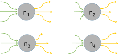
Figure 4: Neurons $n_{1}$ and $n_{3}$ have similar incoming synapses and $n_{1}$ and $n_{4}$ have similar outgoing synapses. In section V we show that in both sigmoid and $\operatorname{ReLU}$ we can remove $n_{3}$, but only in sigmoid can we remove $n_{4}$.

V Proofs for Selecting Input/Output Synapses and Bounding Accuracy Loss

For any given neuron $n$, let $v$ denote the incoming weights which affect the argument of the function, and let $w$ denote the outgoing weights, which are the coefficients applied to the value of the function before being input into the next layer of neurons. We will use $\cdot$ to represent dot product and $\odot$ to represent component-wise multiplication of a vector with a scalar or another vector.

V-A Selecting Input/Output Synapses

Proposition 1.

Let $n_{1}$ and $n_{2}$ be sigmoid neurons, $v_{1}$ and $v_{2}$ their incoming weights and $w_{1}$ and $w_{2}$ their outgoing weights. Then

$$w_{1}\odot\sigma(v_{1}\cdot x)+w_{2}\odot\sigma(v_{2}\cdot x)\approx w\odot\sigma(v\cdot x)$$ (3)

holds for all $x$ if either

1. $v_{1}\approx v_{2}$. Then $w=w_{1}+w_{2}$ and $v=v_{1}$.

2. $w_{1}\approx\alpha w_{2}$. Then $w=w_{1}+w_{2}$ and $v=\frac{\alpha v_{1}+v_{2}}{\alpha+1}$ so long as $\alpha\neq-1$.

Proof.

Equation 3 is a system of equations in $v$ and $w$. If we take a linear approximation of $\sigma$, which is given by $\sigma(x)=\frac{1}{2}+\frac{x}{4}+O(x^{3})$, we transform it into a linear system of equations. Equating constants implies that $w=w_{1}+w_{2}$ (and note that this also means that far from the origin, the approximation error will be very small, because sigmoid has horizontal asymptotes.) Hence:

$$w_{1}\odot v_{1}\cdot x+w_{2}\odot v_{1}\cdot x=(w_{1}+w_{2})\odot v\cdot x$$ (4)

We can solve this for each component of the vector $v$, which gives us

$$v_{k}=\frac{w_{1,j}v_{1,k}+w_{2,j}v_{2,k}}{w_{1,j}+w_{2,j}}$$ (5)

which must hold for all the components $w_{i,j}$ of the vectors $w_{1}$ and $w_{2}$, simultaneously.

Equation 3 is only possible if the $w$’s cancel or if both of them have all entries the same, which is unlikely. The two conditions in the statement, that $v_{1}\approx v_{2}$ or $w_{1}\approx\alpha w_{2}$, both result in cancellations, and upon simplifying, we get the value for $v$ given. ∎

Below, we will compute a bound for the error in the case of similar incoming weights ($v_{1}\approx v_{2}$). The situation for outgoing weights ($w_{1}\approx w_{2}$) is similar, but bounded by larger error in the worst case (proof not included due to space limitations). In practice, though, this bound is not a very tight one. In section VII, we will use both forms of apoptosis for sigmoid neurons, though we remark that this larger error bound does become a problem when attempting to do apoptosis on input features.

The situation for ReLU neurons is simpler. No single ReLU neuron can closely approximate a general sum of two ReLU neurons, an an extreme example of this failure is

$$\operatorname{ReLU}(x)+\operatorname{ReLU}(-x)=|x|.$$ (6)

However, if the two ReLU neurons have incoming weight vectors pointing in almost the same direction, so that one is approximately a positive scalar multiple of the other, we have

Proposition 2.

Let $n_{1},n_{2}$ be ReLU neurons with incoming weights $v_{1},v_{2}$ and outgoing weights $w_{1},w_{2}$. Then, if $v_{2}\approx\alpha v_{1}$ where $\alpha>0$, we have

$$w_{1}\odot\operatorname{ReLU}(v_{1}\cdot x)+w_{2}\odot\operatorname{ReLU}(v_{2}\cdot x) \approx$$ (7)

$$(w_{1}+\alpha w_{2})\odot\operatorname{ReLU}(v_{1}\cdot x)$$ (8)

Proof.

The statement follows from the approximate sequence of equations

$$w_{1}\odot\operatorname{ReLU}(v_{1}\cdot x)+w_{2}\odot\operatorname{ReLU}(v_{2}\cdot x) =$$ (9)

$$w_{1}\odot\max(0,v_{1}\cdot x)+w_{2}\odot\max(0,v_{2}\cdot x) \approx$$ (10)

$$w_{1}\odot\max(0,v_{1}\cdot x)+w_{2}\odot\max(0,\alpha v_{1}\cdot x) =$$ (11)

$$w_{1}\odot\max(0,v_{1}\cdot x)+w_{2}\odot\alpha\max(0,v_{1}\cdot x) =$$ (12)

$$(w_{1}+\alpha w_{2})\odot\max(0,v_{1}\cdot x)$$ (13)

where error is only introduced in the substitution step where $v_{2}$ is replaced by $\alpha v_{1}$. ∎

This situation replaces a pair of half-planes where the neurons are active, with a single half-plane of activity, and because the two half-planes are very close together, this is a good approximation.

The above two propositions show that we can remove sigmoid neurons that have incoming weights nearly identical to another sigmoid neuron. We can also remove sigmoid neurons where outgoing weights are a multiple of the outgoing weights of another neuron (except -1). ReLU neurons whose incoming weights are a positive multiple of those of another may be removed as well, with minimal change to the output function.

V-B Proofs on Error Bounds

In each of these cases, we can understand error bounds for what happens after apoptosis by looking at how different the initial and final output are.

Proposition 3.

Let $v_{1},v_{2}$ be incoming weight vectors, and assume that $|v_{2}-\alpha v_{1}|<\epsilon$ for some $\alpha>0$. Then

$$|\operatorname{ReLU}(v_{1}\cdot x)+\operatorname{ReLU}(v_{2}\cdot x)-(1+\alpha)\operatorname{ReLU}(v_{1}\cdot x)|$$

is at most

$$\max(\alpha|v_{1}||x|,|v_{2}||x|,|x|\epsilon).$$

Proof.

The quantity in question is

$$\operatorname{ReLU}(v_{1}\cdot x)+\operatorname{ReLU}(v_{2}\cdot x)-(1+\alpha)\operatorname{ReLU}(v_{1}\cdot x)$$ (14)

$$\max(0,v_{1}\cdot x)+\max(0,v_{2}\cdot x)-(1+\alpha)\max(0,v_{1}\cdot x)$$ (15)

$$\max(0,v_{2}\cdot x)-\max(0,\alpha v_{1}\cdot x)$$ (16)

Here, we encounter the difficulty of the shape of the $\operatorname{ReLU}$ neuron, and have to do a case study. There are four possibilities:

1. if $v_{2}\cdot x\leq 0$ and $v_{1}\cdot x\leq 0$, then both are zero so the difference is $0$.

2. if $v_{2}\cdot x\leq 0$ and $v_{1}\cdot x\geq 0$, then $\max(0,v_{2}\cdot x)=0$ so the difference is $|\alpha v_{1}\cdot x|\leq\alpha|v_{1}||x|$

3. if $v_{2}\cdot x\geq 0$ and $v_{1}\cdot x\leq 0$, then $\max(0,v_{1}\cdot x)=0$ so the difference is $|v_{2}\cdot x|\leq|v_{2}||x|$

4. if $v_{2}\cdot x\geq 0$ and $v_{1}\cdot x\geq 0$, then the difference is $|v_{2}\cdot x-\alpha v_{1}\cdot x|=|(v_{2}-\alpha v_{1})\cdot x|$, which is $|v_{2}-\alpha v_{1}||x||\cos\theta|$. This is then at most $|x|\epsilon$.

∎

The dependence on $|x|$ in this is a manifestation of the fact that $\operatorname{ReLU}$ does not saturate, and can grow without bound. The worst error regions, though, are where only one of $v_{1}\cdot x$ and $v_{2}\cdot x$ are positive, but these regions are small (measured in angle) because $v_{2}$ closely approximates $\alpha v_{1}$, so they are nearly in the same direction in the first place. The fact that the error can be without bound for arbitrary data does not arise for sigmoid, which saturates.

We note that the same logic as in case 4 of Proposition 3 implies that if $|v_{1}-v_{2}|<\epsilon$, then

$$|v_{1}\cdot x-v_{2}\cdot x|<|x|\epsilon$$ (17)

Proposition 4.

Let $|v_{1}-v_{2}|<\epsilon$. Then

$$|w_{1}\odot\sigma(v_{1}\cdot x)+w_{2}\odot\sigma(v_{2}\cdot x)-(w_{1}+w_{2})\odot\sigma(v_{1}\cdot x)|$$ (18)

is at most

$$\frac{|x||w_{2}|\max\left(|\exp(v_{1}\cdot x)-\exp(v_{1}\cdot x\pm\epsilon|x|)|\right)}{(\exp(v_{1}\cdot x)+1)(\exp(v_{2}\cdot x)+1)}$$ (19)

We note that the factors including $|x|$ in the numerator are dominated by the ones in the denominator, so as expected, for large inputs, the horizontal asymptotes of sigmoid cause the error to be very small.

Proof.

We proceed in stages. First, we note that the terms involving $w_{1}$ cancel, giving us $|w_{2}\odot\sigma(v_{2}\cdot x)-w_{2}\odot\sigma(v_{1}\cdot x)|$. We can pull out the $w_{2}$, to get the quantity $|w_{2}||\sigma(v_{2}\cdot x)-\sigma(v_{1}\cdot x)|$.

As $|v_{1}-v_{2}|<\epsilon$, equation 17 tells us that $|v_{2}\cdot x-v_{1}\cdot x|<|x|\epsilon$. So, if $a=v_{2}\cdot x$ and $b=v_{1}\cdot x$, we must only determine the error in $|\sigma(a)-\sigma(b)|$ for $|a-b|<\epsilon|x|$. But $|\sigma(a)-\sigma(b)|=\frac{|\exp(a)-\exp(b)|}{(\exp(a)+1)(\exp(b)+1)}$, and $|\exp(a)-\exp(b)|$ must at most be $\max(|\exp(b)-\exp(b\pm|x|\epsilon)|)$, because $a$ and $b$ are close together, which gives the result. ∎

Even for a fixed $\epsilon$, this derivation may result in significant error due to the factor of $|w_{2}|$, in practice $|w_{2}|$ will not be so much larger than $|v_{1}|$ and $|v_{2}|$ that the exponentials in the denominator will not cause the error to be small.

In practical use, however, fixing a single $\epsilon$ is suboptimal. This is due in part to the vanishing gradient problem inherent in any back-propagation trained neural network. Because the neurons in different layers will evolve in weight-space at different rates, different values of $\epsilon$ would be needed for each layer. An alternate approach is to define a scaling factor, $f$, and for each neuron $n$ with incoming weights $v$ and outgoing weights $w$, instead of looking for $n^{\prime}$ with $v^{\prime}$ and $w^{\prime}$ such that $|v-v^{\prime}|<\epsilon$ or $|w-w^{\prime}|<\epsilon$, we look for those with $|v-v^{\prime}|<|v|/f$ or $|w-w^{\prime}|<|w|/f$.

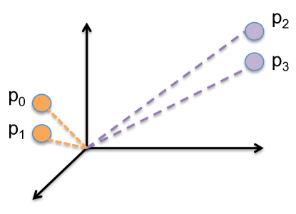
Figure 5: Two pairs of neurons which are unit distance apart, but neurons $p_{2}$ and $p_{3}$ are closer

This handles several problems, most prominently the dimensionality problem. Randomly chosen points are expected to be farther apart in higher dimensional spaces. As they will also be farther from the origin, this also allows the dimension to affect the range being checked for apoptosis.

In Section VII, when we conduct performance evaluation, we will have five levels of apoptosis. The normal level will have angle $f=1.75$. The others will be conservative, very conservative, aggressive and very aggressive, with $f=2,2.5,1.5$ and $1.25$ respectively.

VI Large Scale Parallelization

In this section, we present the solution space in distributed memory implementation – including multi-core and many-core architectures. Our objective is to extract the best possible performance – while leveraging the accelerator based systems (such as GPUs) and traditional multi-core architectures as well, using multi-threading.

Our objective is also to leverage existing Deep Learning software – such as Caffe/TensorFlow/Theano – for our large scale implementations of the proposed heuristics, so that existing optimizations (such as Momentum, AdaGrad, Dropout) can be combined with our own heuristics. We specifically use Caffe, since it is an easily extensible dataflow programming model, with already existing implementations on GPUs using cuDNN and multi-threading implementations for multi-core architectures.

VI-A Caffe Runtime Changes

Caffe sets up a solver and a network, the latter contains the data and the weights of the model whereas the former dictates the rules for performing gradient descent. Our implementation is directly in the Caffe runtime, which speeds up performance significantly compared to implementation in the Python interface.

VI-B Distributed Memory Parallelization

We model our distributed memory implementation on the existing Caffe multi-GPU parallelization. As such, our implementation is based on data parallelism, where the model is replicated and data is distributed, rather than model parallelism, where the model is distributed across multiple nodes. We use MPI [6, 36, 37], which can use high performance interconnects, like InfiniBand, natively, making it suitable for use with supercomputers.

The solver has to be recreated after each apoptosis, but this is not a computationally expensive procedure. Thanks to the use of the Python interface, the data does not need to be loaded every time, which leaves the memory requirements approximately the same as if one solver is used continuously, and cuts the time to recreate the solver down to a negligable factor compared to training time.

VII Performance Evaluation

In this section, we present a detailed evaluation of the proposed heuristics on two InfiniBand clusters – one connected with Intel Haswell CPUs and other connected with nVIDIA Tesla K40m GPUs.

VII-A Hardware and Software Details

VII-A1 Hardware

Our Testbed consists of 27 compute nodes, where each compute node has two sockets, and each socket is 10-core Intel(R) Xeon(R) CPU E5-2680 v2 @ 2.80GHz. Each compute node is connected with 750 GB of main memory, and InfiniBand QDR interconnect. Six compute nodes are also connected with nVIDIA Tesla k40m GPUs. We refer to our multi-core cluster as CPU cluster and other testbed as GPU cluster.

VII-A2 Software

We use OpenMPI v1.8.3 for performance evaluation with Intel compiler 16.0.1. For using GPUs, we use cuDNN v3, CUDA v7.0.28, and a version of Caffe modified to work with MPI.

VII-B Datasets

We consider several well studied datasets for performance evaluation. Our primary large datasets are Higgs Boson [4] classification dataset (11M samples) and well studied ImageNet [2] classification datasets ($\approx$1.3M images). The evaluation also includes Handwritten Digits recognition (MNIST) to establish a baseline.

VII-C MNIST

MNIST is a well studied dataset in literature. We use MNIST as one of the prominent datasets for studying the impact of a large combination of heuristics proposed in section IV. We also study the scaling effect on CPU and GPU cluster. For scaling, we utilize two main changes: 1) A single process per and several threads per node for better memory utilization and lesser replication of model 2) Higher learning rate (0.1) to mitigate the effect of averaging the weights across compute nodes.

Figures 6 and 7 show the results for CPU and GPU clusters respectively. In Figure 6, we observe an overall speedup of 3.2x in comparison to default algorithm with Normal apoptosis – with no loss of accuracy and 11x reduction in parameters. The speedup and parameter reduction for aggressive apoptosis is higher, but it leads to a loss of more than 5% accuracy – so we do not consider it as a viable alternative. We observe an accuracy of 96.5-97% accuracy for each of these executions (except aggressive) – which matches with well published literature for DNN and MNIST. For evaluation with CNN, we use our GPU cluster as shown in Figure 7. We use 6 GPUs and compare the speedup and parameter reduction. We observe a 3x reduction in parameters for normal apoptosis, accuracy $\approx$ 99.2% – which is state of the art for CNN executions.

Using MNIST as a reference set, for rest of the evaluation, we use quarter-life with logarithmic subsequent apoptosis, and fixed degree of apoptosis. Unless specified otherwise, we use normal factor (1.75) for apoptosis.

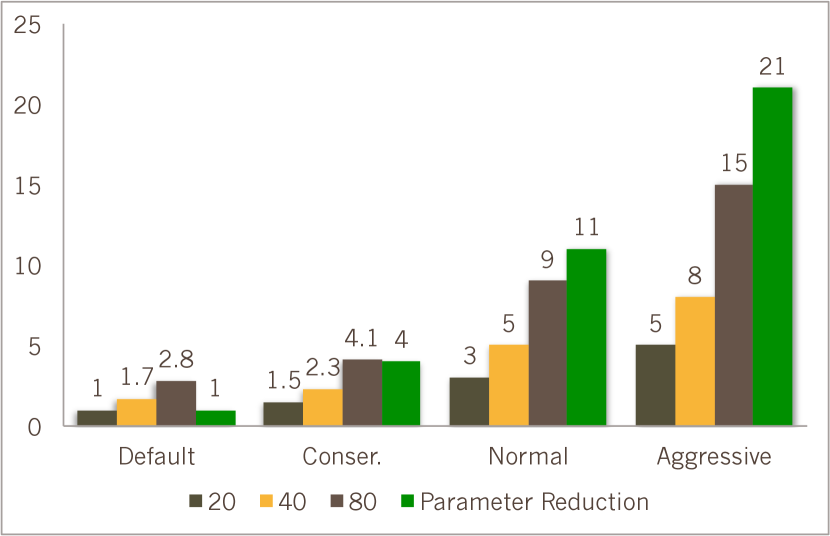
Figure 6: Relative Speedup and Parameter Reduction to Default using DNN with 512x512 network with MNIST

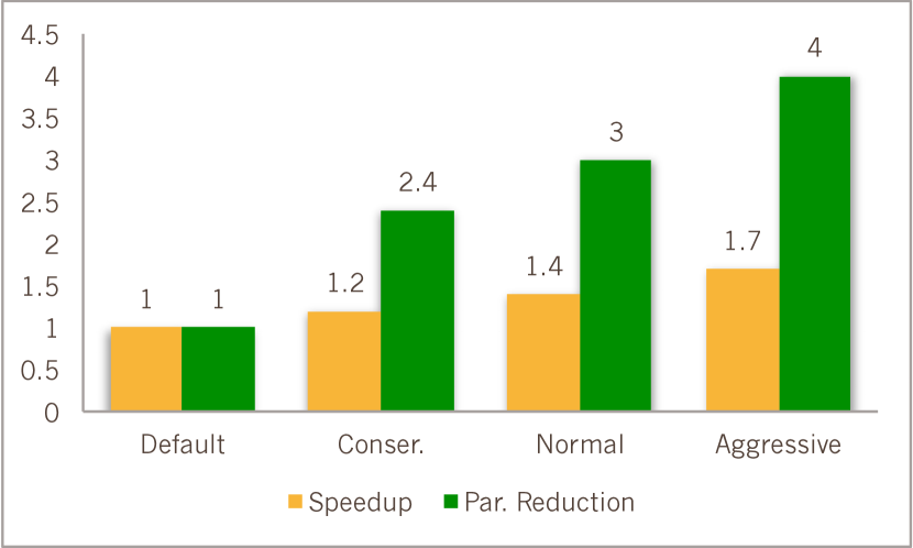
Figure 7: Relative Speedup and Parameter Reduction using CNN with 32x64 Conv. Layers and 256 Fully connected layer network with MNIST and 6 GPUs

VII-D Higgs Boson Particle Classification

The Higgs Boson particle classification dataset is a critical dataset used for model generation and discovery of exotic particles. Sadowski et al. published and studied the dataset with Deep Learning algorithms using a three layer DNN (500x500x500) network with neuron dropout [4]. Our objective with this workload is two-fold: 1) Reduce the training time to learn the model, while conducting neuron apoptosis 2) maintaining – and possibly improving – accuracy (measured using area under curve (AUC), which is the probability that a randomly selected positive sample will be rated higher than a randomly selected negative example), as suggested by Sadowski et al.. For this purpose, we start with a bigger network to possibly improve accuracy – while utilizing apoptosis to remove redundant neurons. We execute this dataset using up to 540 cores.

Figure 8 shows the results. With aggressive apoptosis, we are able to observe a speedup of 6x – while no reduction in Area Under Curve (AUC). We match the AUC reported by Sadowski et al. [4], while providing a huge speedup.

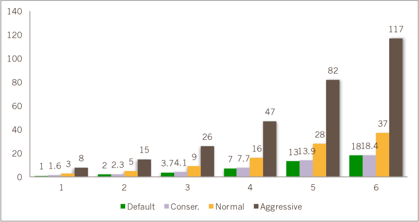
Figure 8: Higgs Boson Relative Performance to 1 Node using up to 540 cores (One node has 20 cores) with 512x512x512 network

VII-D1 Science Results with Neuron Apoptosis

The peak AUC reported by Sadowski et al. is 0.88/1. However, we wanted to understand whether it is possible to create a neural network topology – which can provide better prediction for a scientist for separating Higgs Boson particle from other particles. We used a deeper network than ever considered before with Higgs by using a 512x512x512x512 network. Being a 4 layer network, we used autoencoders for learning weights layer by layer, conducted training on the output layer and compared the results for apoptosis and the default algorithm.

Our evaluation indicates major contribution to the field: 1) Using deeper networks, our AUC is 0.94/1 – which is 6 percentage points better than previously published result 2) With proposed apoptosis, we reduce number of parameters by 3x in comparison to the parameters in the best known AUC for Higgs Boson particle classification – while achieving a speedup of 2.44x in comparison to the no apoptosis algorithm.

VII-E ImageNet - ILSVRC12 Results

In this section, we present results for ImageNet Large Scale Visualization Research Challenge (ILSVRC12). The objective of this evaluation is to compare the accuracy reported by several neural networks – including DNN and CNN networks – after a fixed training time provided to each of the approaches. ILSVRC12 consists of 1.3M images, each of which is labeled in one of the 1000 categories. The ultimate objective of the challenge is to improve the classification accuracy – or reduce the time to solution to achieve a given accuracy. We primarily use GPU cluster for ImageNet evaluation – especially since cuDNN is heavily optimized in comparison to CPU based implementation.

During this investigation, we discovered that, although the standard method of training AlexNet [38] calls for 360000 iterations through the dataset, if we use an exponentially decaying learning rate with multiplicative factor 0.999964, the model converges after only 60000 iterations. We used this “quick” AlexNet solver in the evaluation below, along with optimization by using as many as 8 GPUs.

For each non-AlexNet execution, we provide a training time of eight hours using 6 GPUs. We observed the following points: 1) DNN provided significant reduction in parameters, with negligible accuracy loss, while providing speedup 2) With CNN, the primary apoptosis is observed at the conjunction of the convolution and fully connected layers. However, most of the time is spent in convolutions, and hence the speedup is lesser than the DNN networks.

TABLE I: ImagaNet Evaluation. First column shows the Deep Learning algorithm used; second shows the sizes of hidden layers; third the relative reduction in parameters; fourth change in accuracy and fifth the speedup

Algo	Network	Pa. Red.	Acc. (%)	Speedup
DNN	2048,2048	27x	$-0.7$	2.1x
DNN	4096	34x	$-0.5$	2.3x
CNN	64,128 and 2048	18x	$-0.3$	1.2x

For AlexNet, we trained using our improved solver for various levels of aggressiveness of Apoptosis. For this network, the results were mixed. For most apoptosis factors, either virtually no ($\leq 1\%$) of parameters were removed, or else the vast majority ($\geq 99.9\%$) were, and so obtained either no speedup or else an extreme loss of accuracy. For factor $1.35$, however, $72.48\%$ of the parameters were removed, leading to a speedup of 2.6x/iteration. However, while this reduced model recovered the accuracy from before apoptosis, but did not, during the life of the quick solver, converge to the usual test accuracy of $54\%$.

VII-F Discussion

There are a few important observation from the previous sections: 1) In many cases, adaptive apoptosis results in significant reduction of parameters and improvement in training time 2) In case of Higgs Boson dataset, we observed that deeper networks – with lesser parameters than the original network – produced better results. We also observed a conical shape with reducing neurons per layer (starting from input layer and ending at the output layer) in the neural network topology after apoptosis. This can be explained by the fact that number of features is much higher than the number of classes.

An important discussion is the guidance for future users of this research. An advantage of the proposed methodology is that a user may start with a very large network to build models for its dataset, and expect that the apoptosis would remove redundant neurons – while gaining speedup, and possibly accuracy, especially if the stopping criteria is fixed time/epochs. This is attractive for novice and advanced users alike, as there is little guidance on specification of neural network topology. The proposed approach generates a much smaller, near optimal topology, which would be sufficient for the user.

VIII Conclusions

In this paper, we have presented novel techniques to adaptively remove redundant neurons (neuron apoptosis) for accelerating Deep Learning algorithms (Deep Neural Networks, Convolutional Neural Networks and Autoencoders) – during the training phase itself on large scale systems. The proposed techniques are in sharp contrast with existing approaches [10], which require a re-training phase for removing the weights which do not contribute – resulting in a significant slowdown (2.5x reported by Han et al [10]) of the training time.

Our contributions in this paper include novel heuristics for deciding on initial apoptosis, subsequent apoptosis and degree of apoptosis during the training phase itself. We provide theoretical underpinnings to study the apoptosis for several neuron types, consider apoptosis for input/output synapses for several neuron types and provide proofs on bounding accuracy loss with apoptosis. We implement our proposed heuristics using Caffe, by extending it to use MPI and allow multi-node training. We evaluate our proposed heuristics with several large datasets including Higgs Boson particle dataset, ImageNet classification and MNIST handwritten digit recognition. We use two clusters – one connected with Intel Haswell CPU and InfiniBand QDR and other connected with nVIDIA GPUs and InfiniBand. Our evaluation indicates significant improvement in multiple dimensions – including a reduction in parameters by 30x, and 2-3x speedup in time comparison to no apoptosis implementation. A major contribution of our paper is also an improvement in classification accuracy for Higgs Boson particle dataset, by using apoptosis on a Deeper network than published architecture. We are able to improve the Area Under Curve (AUC), by 6 percentage points from best known result 0.88/1 to 0.94/1, while reducing the number of parameters by 3x in comparison to best result producing network [4] and achieving a 2.44x speedup.

References

- [1] J. Dean, G. Corrado, R. Monga, K. Chen, M. Devin, Q. V. Le, M. Z. Mao, M. Ranzato, A. W. Senior, P. A. Tucker, K. Yang, and A. Y. Ng, “Large scale distributed deep networks,” in Advances in Neural Information Processing Systems 25: 26th Annual Conference on Neural Information Processing Systems 2012. Proceedings of a meeting held December 3-6, 2012, Lake Tahoe, Nevada, United States., 2012, pp. 1232–1240. [Online]. Available: http://papers.nips.cc/paper/4687-large-scale-distributed-deep-networks
- [2] A. Krizhevsky, I. Sutskever, and G. E. Hinton, “Imagenet classification with deep convolutional neural networks,” in Advances in Neural Information Processing Systems 25: 26th Annual Conference on Neural Information Processing Systems 2012. Proceedings of a meeting held December 3-6, 2012, Lake Tahoe, Nevada, United States., 2012, pp. 1106–1114. [Online]. Available: http://papers.nips.cc/paper/4824-imagenet-classification-with-deep-convolutional-neural-networks
- [3] A. Graves and J. Schmidhuber, “Framewise phoneme classification with bidirectional LSTM and other neural network architectures,” Neural Networks, vol. 18, no. 5-6, pp. 602–610, 2005. [Online]. Available: http://dx.doi.org/10.1016/j.neunet.2005.06.042
- [4] P. J. Sadowski, D. Whiteson, and P. Baldi, “Searching for higgs boson decay modes with deep learning,” in Advances in Neural Information Processing Systems 27: Annual Conference on Neural Information Processing Systems 2014, December 8-13 2014, Montreal, Quebec, Canada, 2014, pp. 2393–2401. [Online]. Available: http://papers.nips.cc/paper/5351-searching-for-higgs-boson-decay-modes-with-deep-learning
- [5] G. E. Hinton, O. Vinyals, and J. Dean, “Distilling the knowledge in a neural network,” CoRR, vol. abs/1503.02531, 2015. [Online]. Available: http://arxiv.org/abs/1503.02531
- [6] A. Vishnu, C. Siegel, and J. Daily, “Distributed TensorFlow with MPI,” ArXiv e-prints, Mar. 2016.
- [7] S. Hochreiter, “The vanishing gradient problem during learning recurrent neural nets and problem solutions,” Int. J. Uncertain. Fuzziness Knowl.-Based Syst., vol. 6, no. 2, pp. 107–116, Apr. 1998. [Online]. Available: http://dx.doi.org/10.1142/S0218488598000094
- [8] N. Srivastava, G. Hinton, A. Krizhevsky, I. Sutskever, and R. Salakhutdinov, “Dropout: A simple way to prevent neural networks from overfitting,” Journal of Machine Learning Research, vol. 15, pp. 1929–1958, 2014. [Online]. Available: http://jmlr.org/papers/v15/srivastava14a.html
- [9] Z. Yang, M. Moczulski, M. Denil, N. de Freitas, A. Smola, L. Song, and Z. Wang, “Deep fried convnets,” in International Conference on Computer Vision (ICCV), 2015.
- [10] S. Han, J. Pool, J. Tran, and W. Dally, “Learning both weights and connections for efficient neural network,” in Advances in Neural Information Processing Systems 28, C. Cortes, N. D. Lawrence, D. D. Lee, M. Sugiyama, and R. Garnett, Eds. Curran Associates, Inc., 2015, pp. 1135–1143. [Online]. Available: http://papers.nips.cc/paper/5784-learning-both-weights-and-connections-for-efficient-neural-network.pdf
- [11] F. N. Iandola, M. W. Moskewicz, K. Ashraf, S. Han, W. J. Dally, and K. Keutzer, “Squeezenet: Alexnet-level accuracy with 50x fewer parameters and <1mb model size,” CoRR, vol. abs/1602.07360, 2016. [Online]. Available: http://arxiv.org/abs/1602.07360
- [12] F. N. Iandola, K. Ashraf, M. W. Moskewicz, and K. Keutzer, “Firecaffe: near-linear acceleration of deep neural network training on compute clusters,” CoRR, vol. abs/1511.00175, 2015. [Online]. Available: http://arxiv.org/abs/1511.00175
- [13] Y. Jia, E. Shelhamer, J. Donahue, S. Karayev, J. Long, R. Girshick, S. Guadarrama, and T. Darrell, “Caffe: Convolutional architecture for fast feature embedding,” arXiv preprint arXiv:1408.5093, 2014.
- [14] F. Bastien, P. Lamblin, R. Pascanu, J. Bergstra, I. J. Goodfellow, A. Bergeron, N. Bouchard, and Y. Bengio, “Theano: new features and speed improvements,” Deep Learning and Unsupervised Feature Learning NIPS 2012 Workshop, 2012.
- [15] J. Bergstra, O. Breuleux, F. Bastien, P. Lamblin, R. Pascanu, G. Desjardins, J. Turian, D. Warde-Farley, and Y. Bengio, “Theano: a CPU and GPU math expression compiler,” in Proceedings of the Python for Scientific Computing Conference (SciPy), Jun. 2010, oral Presentation.
- [16] R. Collobert, S. Bengio, and J. Marithoz, “Torch: A modular machine learning software library,” 2002.
- [17] M. Abadi, A. Agarwal, P. Barham, E. Brevdo, Z. Chen, C. Citro, G. S. Corrado, A. Davis, J. Dean, M. Devin, S. Ghemawat, I. Goodfellow, A. Harp, G. Irving, M. Isard, Y. Jia, R. Jozefowicz, L. Kaiser, M. Kudlur, J. Levenberg, D. Mané, R. Monga, S. Moore, D. Murray, C. Olah, M. Schuster, J. Shlens, B. Steiner, I. Sutskever, K. Talwar, P. Tucker, V. Vanhoucke, V. Vasudevan, F. Viégas, O. Vinyals, P. Warden, M. Wattenberg, M. Wicke, Y. Yu, and X. Zheng, “TensorFlow: Large-scale machine learning on heterogeneous systems,” 2015, software available from tensorflow.org. [Online]. Available: http://tensorflow.org/
- [18] M. Bianchini and F. Scarselli, “On the complexity of neural network classifiers: A comparison between shallow and deep architectures,” IEEE Transactions on Neural Networks and Learning Systems, vol. 25, no. 8, pp. 1553 – 1565, 2014.
- [19] G. E. Hinton and S. Osindero, “A fast learning algorithm for deep belief nets,” Neural Computation, vol. 18, p. 2006, 2006.
- [20] Y. Bengio, P. Lamblin, D. Popovici, and H. Larochelle, “Greedy layer-wise training of deep networks,” in Advances in Neural Information Processing Systems 19, B. Schölkopf, J. C. Platt, and T. Hoffman, Eds. MIT Press, 2007, pp. 153–160. [Online]. Available: http://papers.nips.cc/paper/3048-greedy-layer-wise-training-of-deep-networks.pdf
- [21] G. E. Hinton and R. R. Salakhutdinov, “Reducing the dimensionality of data with neural networks,” Science, vol. 313, no. 5786, pp. 504–507, Jul. 2006. [Online]. Available: http://www.ncbi.nlm.nih.gov/sites/entrez?db=pubmed&uid=16873662&cmd=showdetailview&indexed=google
- [22] P. Vincent, H. Larochelle, I. Lajoie, Y. Bengio, and P.-A. Manzagol, “Stacked denoising autoencoders: Learning useful representations in a deep network with a local denoising criterion,” J. Mach. Learn. Res., vol. 11, pp. 3371–3408, Dec. 2010. [Online]. Available: http://dl.acm.org/citation.cfm?id=1756006.1953039
- [23] R. A. Chambers, M. N. Potenza, R. E. Hoffman, and W. Miranker, “Simulated apoptosis/neurogenesis regulates learning and memory capabilities of adaptive neural networks,” Neuropsychopharmacology, vol. 29, no. 4, pp. 747–758, 2004.
- [24] J. Sietsma and R. J. Dow, “Neural net pruning-why and how,” in Neural Networks, 1988., IEEE International Conference on. IEEE, 1988, pp. 325–333.
- [25] R. Reed, “Pruning algorithms-a survey,” Trans. Neur. Netw., vol. 4, no. 5, pp. 740–747, Sep. 1993. [Online]. Available: http://dx.doi.org/10.1109/72.248452
- [26] S. M. Kamruzzaman and A. R. Hasan, “Pattern classification using simplified neural networks,” CoRR, vol. abs/1009.4983, 2010. [Online]. Available: http://arxiv.org/abs/1009.4983
- [27] A. N. Gorban, E. M. Mirkes, and V. G. Tsaregorodtsev, “Generation of explicit knowledge from empirical data through pruning of trainable neural networks,” in Neural Networks, 1999. IJCNN’99. International Joint Conference on, vol. 6. IEEE, 1999, pp. 4393–4398.
- [28] G. E. Hinton, N. Srivastava, A. Krizhevsky, I. Sutskever, and R. R. Salakhutdinov, “Improving neural networks by preventing co-adaptation of feature detectors,” arXiv preprint arXiv:1207.0580, 2012.
- [29] B. Goodrich and I. Arel, “Neuron clustering for mitigating catastrophic forgetting in feedforward neural networks,” in Computational Intelligence in Dynamic and Uncertain Environments (CIDUE), 2014 IEEE Symposium on. IEEE, 2014, pp. 62–68.
- [30] W. Chen, J. T. Wilson, S. Tyree, K. Q. Weinberger, and Y. Chen, “Compressing neural networks with the hashing trick,” CoRR, vol. abs/1504.04788, 2015. [Online]. Available: http://arxiv.org/abs/1504.04788
- [31] K. Murray and D. Chiang, “Auto-sizing neural networks: With applications to n-gram language models,” arXiv preprint arXiv:1508.05051, 2015.
- [32] H. Hu, R. Peng, Y.-W. Tai, and C.-K. Tang, “Network trimming: A data-driven neuron pruning approach towards efficient deep architectures,” arXiv preprint arXiv:1607.03250, 2016.
- [33] Y. LeCun, L. Bottou, Y. Bengio, and P. Haffner, “Gradient-based learning applied to document recognition,” Proceedings of the IEEE, vol. 86, no. 11, pp. 2278–2324, 1998.
- [34] H. Lee, R. Grosse, R. Ranganath, and A. Y. Ng, “Convolutional deep belief networks for scalable unsupervised learning of hierarchical representations,” in Proceedings of the 26th Annual International Conference on Machine Learning. ACM, 2009, pp. 609–616.
- [35] F. N. Iandola, K. Ashraf, M. W. Moskewicz, and K. Keutzer, “Firecaffe: near-linear acceleration of deep neural network training on compute clusters,” arXiv preprint arXiv:1511.00175, 2015.
- [36] W. Gropp, E. Lusk, N. Doss, and A. Skjellum, “A High-Performance, Portable Implementation of the MPI Message Passing Interface Standard,” Parallel Computing, vol. 22, no. 6, pp. 789–828, 1996.
- [37] A. Geist, W. Gropp, S. Huss-Lederman, A. Lumsdaine, E. L. Lusk, W. Saphir, T. Skjellum, and M. Snir, “MPI-2: Extending the message-passing interface,” in Euro-Par, Vol. I, 1996, pp. 128–135.
- [38] A. Krizhevsky, I. Sutskever, and G. E. Hinton, “Imagenet classification with deep convolutional neural networks,” in Advances in Neural Information Processing Systems 25, F. Pereira, C. Burges, L. Bottou, and K. Weinberger, Eds. Curran Associates, Inc., 2012, pp. 1097–1105. [Online]. Available: http://papers.nips.cc/paper/4824-imagenet-classification-with-deep-convolutional-neural-networks.pdf