A Note On The Semiclassical Formulation Of BPS States In Four-Dimensional N=2 Theories

Abstract:

Vector spaces of (framed) BPS states of Lagrangian four-dimensional N=2 field theories can be defined in semiclassical chambers in terms of the $L^{2}$-cohomology of Dirac-like operators on monopole moduli spaces. This was spelled out in [20, 21] for theories with only vectormultiplets, taking into account only a subset of the possible half-supersymmetric ’t Hooft-Wilson line defects. This note completes the discussion by describing the modifications needed when including matter hypermultiplets together with arbitrary ’t Hooft-Wilson line defects. Two applications of this extended discussion are given.

MnLargeSymbols’164 MnLargeSymbols’171

1 Introduction And Conclusion

This note summarizes part of a talk delivered by one of us at the Nambu Memorial Symposium at the University of Chicago, March 2016. Professor Nambu’s profound contributions to the theory of spontaneous symmetry breaking and to the use of nonabelian gauge theory in particle physics firmly establishes him as one of the great physicists of the twentieth century. This note is about the theory of magnetic monopoles. As far as we know, Professor Nambu never wrote a paper about magnetic monopoles, but given that these are a beautiful and important aspect of spontaneously broken nonabelian gauge theories the topic seems to us to be most apt as a contribution to this memorial volume for Professor Nambu.

BPS states [23, 30] (and their framed analogues [13]) in four-dimensional N=2 supersymmetric field theories can be defined in the semiclassical limit in terms of $L^{2}$ cohomology of Dirac-like operators on moduli spaces of (singular) monopoles, as is well-known from a rather extensive previous literature. Some finishing touches of this formulation were recently worked out in [20] but only for pure gauge theories, and only for framed BPS states in the presence of a subset of the possible ’t Hooft-Wilson line defects. This note extends the finishing touches of [20] to include theories with arbitrary hypermultiplet representations together with arbitrary ’t Hooft-Wilson line defects. The main modification is that the Dirac operator must be coupled to a hyperholomorphic vector bundle. The relevant hyperholomorphic bundle is described in section 3 and is derived from the universal bundle of Atiyah and Singer [2]. The proof of the main claim follows easily by constructing the relevant N=4 supersymmetric quantum mechanics on monopole moduli space, following [9, 10, 11, 12, 21, 25, 26, 29]. Some details are in appendix B.

There are two applications of this work. First, given the truth of the no-exotics conjecture of [13] (partially proven in [4, 5, 8]), the arguments here complete the proof of the Generalized Sen Conjecture described in section 4 below and in section 4.1 of [20]. Second, as in [21], when combined with explicit computations from [13] we obtain a wealth of predictions for the $L^{2}$ kernels of Dirac operators on (singular) monopole moduli spaces. The novel point in this note is that these predictions are extended to Dirac operators coupled to certain hyperholomorphic bundles described below. One example is worked out in detail in section 5.

This paper builds on and extends the letter [20]. We will endeavor to use the same notation as in that letter and in the interest of brevity we will not always fully define notation - so we we will assume the reader has some familiarity with [20]. Full computations and complete details can be found in the forthcoming PhD thesis of the first author. Further background material and extensive references to the large literature on the semiclassical formulation of BPS states can be found in [21, 29].

2 Statement And Solution Of The Problem

We wish to describe BPS states in a semiclassical limit, allowing for the presence of arbitrary ’t Hooft-Wilson line defects. We thus confine attention to Lagrangian d=4 N=2 theories. These are described by the following data:

1. Gauge group and couplings: A semisimple compact Lie group $G$ together with a complex gauge coupling $\tau$ for each simple factor of $G$.

2. Matter hypermultiplets: A quaternionic representation ${\cal R}$ of $G$ compatible with a positive inner product on ${\cal R}$. (Thus, all the complex structures are orthogonal transformations of ${\cal R}$.)

3. Mass parameters: The flavor group $G_{f}$ is defined to be the commutant of $G$ in the orthogonal group $O({\cal R})$ preserving the inner product on ${\cal R}$. The mass parameters $m$ are valued in $\mathfrak{g}_{f}\otimes\mathbb{C}$ where $\mathfrak{g}_{f}$ is the Lie algebra of $G_{f}$. Then N=2 supersymmetry requires $[m,m^{\dagger}]=0$. Hence we can assume that $m\in\mathfrak{t}_{f}\otimes\mathbb{C}$ is in a Cartan subalgebra of $G_{f}$. We will further assume that it is a regular element so that the flavor symmetry group is broken to a maximal torus $\cong U(1)^{N_{f}}$ by the masses.

A quick and elegant way to understand that this is the appropriate way to formulate mass parameters is to use the viewpoint [1, 24] that $m$ are the vev’s of adjoint scalars of vectormultiplets when the flavor group $G_{f}$ is weakly gauged (i.e. the flavor gauge coupling is taken to zero). The vacuum condition for these scalars is simply $[m,m^{\dagger}]=0$.

Next we need the data defining half-supersymmetric ’t Hooft-Wilson line defects. These are determined by the data:

1. Unbroken supersymmetry: A choice of phase $\zeta\in U(1)$ (or rather a lift of $\zeta$ to the universal cover of $U(1)$) specifying which four supersymmetries of the half-supersymmetric defect remain unbroken. For details see [13, 15].

2. ’t Hooft-Wilson charges: An equivalence class of a pair $[P,Q]$ where $P$ is a cocharacter of $G$ and $Q$ is a weight of the centralizer $Z(P)\subset G$. The square brackets indicate the equivalence class under the diagonal action of the Weyl group of $G$. Using this data we can define defect boundary conditions on the field in the path integral [14].

We denote the line defect determined by the above data by $L_{\zeta}[P,Q]$.

Finally, we need infrared data. These consist of

1. A Coulomb branch vacuum: The Coulomb branch is ${\cal B}:=\mathfrak{t}\otimes\mathbb{C}/W$ where $\mathfrak{t}$ is a Cartan subalgebra of $\mathfrak{g}={\rm Lie}(G)$. A typical point is traditionally denoted $u\in{\cal B}$. The “semiclassical region” is a set of regions where $u\to\infty$ on the Coulomb branch. The precise definition can be found in section 4.6 of [21] but the basic idea is very simple: One takes the bare coupling constant to zero and hence ${\rm Im}(\tau)\to\infty$ for each simple factor of $G$. A point $u$ on the Coulomb branch vacuum determines a vacuum expectation value $X_{\infty}\in\mathfrak{g}$ of a Higgs field $X$ up to conjugation. (The field $X$ is defined in equation (54).) We will assume $X_{\infty}$ is a regular element of $\mathfrak{g}$ and hence determines a Cartan subalgebra $\mathfrak{t}$, a Cartan subgroup $T\subset G$, and a set of positive roots.

2. An infrared charge: The mass parameters and vacuum expectation value $X_{\infty}$ break the $G_{f}\times G$ symmetry to an abelian group. Taking into account dual magnetic symmetries, the symmetry group of the IR theory is a torus $\tilde{T}$ that fits in an exact sequence

   $$1\rightarrow T_{em}\rightarrow\tilde{T}\rightarrow T_{f}\rightarrow 1.$$ (1)

   Here $T_{f}$ is the Cartan subgroup of the flavor group while $T_{em}$ is the group of electric and magnetic gauge transformations. The IR charges, $\gamma$, are in the character lattice $\Gamma$ of $\tilde{T}$ and hence also fit in a sequence:

   $$0\rightarrow\Gamma_{f}\rightarrow\Gamma\rightarrow\Gamma_{em}\rightarrow 0.$$ (2)

   Here the lattice of flavor charges $\Gamma_{f}$ is just the character lattice of the unbroken flavor symmetry $T_{f}$ while $\Gamma_{em}$ is the symplectic lattice of electric and magnetic gauge charges. The above sequences split, but in general not naturally since one can add a gauge current to a flavor current.

Given the above data one can formulate the general problem: Define and compute the vector space of framed BPS states for the theory in question with the specified IR data. This is an extremely difficult problem and has been the subject of much research. However, when $u$ is in a weak-coupling region the problem is much more manageable, although it still requires a little attention to give a precise statement. The full solution to the semiclassical version of this problem is the subject of this note.

When the problem is restricted to theories consisting only of vectormultiplets, together with a subset of the possible ’t Hooft-Wilson line defects (this subset includes $L_{\zeta}[P,0]$ for all $P$) the solution was explained in [20, 21]. We summarize the answer very briefly. To begin, in the semiclassical regime there is a distinguished family of duality frames, all related by the Witten effect. There is a canonical splitting of (2) (up to the Witten effect) which allows us to decompose a charge $\gamma\in\Gamma$ as

$$\gamma=\gamma_{f}\oplus\gamma_{m}\oplus\gamma_{e}\in\Lambda_{wt,f}\oplus\Lambda_{mw}\oplus\Lambda_{wt}.$$ (3)

We will denote $\gamma_{e+f}:=\gamma_{f}\oplus\gamma_{e}$ below. The Witten effect arises from monodromy defined by a map $\Lambda_{mw}\rightarrow\Lambda_{wt,f}\oplus\Lambda_{wt}$, but the magnetic charge $\gamma_{m}$ is invariant in the semiclassical regime.

In the semiclassical region it is useful to define a pair of “real” adjoint vevs [21]

$$\begin{split}{\cal X}&:={\rm Im}(\zeta^{-1}a(u))\in\mathfrak{t}\\ {\cal Y}&:={\rm Im}(\zeta^{-1}a_{D}(u))\in\mathfrak{t}\\ \end{split}$$ (4)

where $a(u)$ and $a_{D}(u)$ are the periods relative to the canonical weak coupling duality frame and ${\cal X}=X_{\infty}+\cdots$ to leading order in the weak coupling expansion. When there is no line defect we apply the same formula with $\zeta=-Z^{cl}/|Z^{cl}|$ in the weak coupling limit (see equation (56) below).

Using the vev ${\cal X}$ and the magnetic charge $\gamma_{m}$ we can define a moduli space of (possibly singular) magnetic monopoles. Then, the semiclassical dynamics of BPS states with magnetic charge $\gamma_{m}$ are described by collective coordinates on the moduli space. These collective coordinates are governed by an N=4 supersymmetric quantum mechanics, and one of the supersymmetry operators is the Dirac operator

$$\not{D}^{\cal Y}=\not{D}+\not{{\mathrm{G}}}({\cal Y})$$ (5)

where $\not{D}$ is the ordinary Dirac operator acting on Dirac spinors on $\overline{\underline{{\cal M}}}$ or ${\cal M}$ and $\not{{\mathrm{G}}}({\cal Y})$ is Clifford multiplication by the hyperholomorphic vector field associated with global gauge transformations by ${\cal Y}\in\mathfrak{t}$. One then defines the space of all framed BPS states with fixed magnetic charge $\gamma_{m}$, in the presence of the line defect $L_{\zeta}[P,0]$, to be the $L^{2}$ kernel, denoted here by ${\cal K}$, of the operator $\not{D}^{{\cal Y}}$ on $\overline{\underline{{\cal M}}}([P],\gamma_{m};{\cal X})$:

$${\cal K}:={\rm ker}_{L^{2}}\not{D}^{{\cal Y}}.$$ (6)

The space ${\cal K}$ is a representation of a group isomorphic to

$$T\times SO(3)_{\rm rotation}\times SU(2)_{R},$$ (7)

where $T$ is the maximal torus of $G$ determined by the commutant of the regular vev ${\cal X}$, $SO(3)_{\rm rotation}$ is the group of rotations around some point in spatial ${\mathbb{R}}^{3}$, and $SU(2)_{R}$ is the commutant of the symplectic holonomy of the hyperkähler metric. The group $SU(2)_{R}$ has a lift to the spin bundle and preserves ${\cal K}$. The group $SO(3)_{\rm rotation}$ induces a group of isometries of the hyperkähler metric and again preserves ${\cal K}$. Finally, global gauge transformations by $T$ are hyperholomorphic and commute with $\not{D}^{\cal Y}$. The isotypical subspaces of ${\cal K}$, when decomposed as a $T$-representation, are identified with the subspaces of framed BPS states of definite electric charge. They therefore are in representations of $SO(3)_{\rm rotation}\times SU(2)_{R}$.

Now, the modification of the above answer in the case where we include general ’t Hooft-Wilson lines (including the possibility $P=0$ and $Q\not=0$, i.e. general Wilson lines) as well as general matter hypermultiplets is very simple. One defines an Hermitian hyperholomorphic vector bundle ${\cal E}_{\rm line}$ associated with the line defects together with a hyperholomorphic bundle ${\cal E}_{\rm matter}$ associated with the quaternionic representation ${\cal R}$. Then we simply use the same Dirac operator as before coupled to

$${\cal E}={\cal E}_{\rm line}\otimes{\rm Spin}({\cal E}_{\rm matter})$$ (8)

where ${\rm Spin}({\cal E}_{\rm matter})$ is a vector bundle associated to the spin bundle of ${\cal E}_{\rm matter}$. The bundle ${\cal E}_{\rm matter}$ represents hypermultiplet fermion degrees of freedom in the supersymmetric quantum mechanics of appendix B and, upon quantization of the Clifford algebra based on ${\cal E}_{\rm matter}$, we obtain states in the spin representation. The bundle ${\cal E}$ inherits a hyperholomorphic connection from the ones on ${\cal E}_{\rm line}$ and ${\cal E}_{\rm matter}$. These bundles and connections are defined in section 3 below. To define (framed) BPS states of definite magnetic charge we take the $L^{2}$ kernel of this operator on $\overline{\underline{{\cal M}}}$ if $P\not=0$ and on ${\cal M}$ if $P=0$ but $Q\not=0$. If there are no line defects we must take the $L^{2}$ kernel on the strongly-centered moduli space (a factor of the univeral cover) and impose an equivariance condition under the action of the Deck group on the universal cover. These complications are explained at length in [20, 21] and no new issues arise in the more general situation we consider here.

Once again, the torus $T_{f}\times T$ of the unbroken flavor and gauge symmetry acts on the bundle ${\cal E}$ and commutes with the Dirac operator. Therefore the $L^{2}$-kernel is a representation of

$$T_{f}\times T\times SO(3)_{\rm rotation}\times SU(2)_{R}.$$ (9)

The flavor and electric charges are determined by the character of $T_{f}\times T$ acting on the kernel. The desired space of BPS states is the isotypical subspace:

$$\overline{\underline{{\cal H}}}(L_{\zeta}[P,Q];\gamma;u):={\rm ker}_{L^{2}}^{\gamma_{e+f}}(\not{D}^{\cal Y})$$ (10)

in the framed case, with a similar equation for the vanilla case (i.e. without line defects).

3 Construction Of The Hyperholomorphic Bundles

3.1 Hyperholomorphic Bundles Associated To Line Defects

We suppose a line defect $L_{\zeta}[P,Q]$ has been inserted at a point $\vec{x}\in{\mathbb{R}}^{3}$. Let ${\cal Q}$ denote the universal principal $Z(P)$-bundle of appendix A over ${\mathbb{R}}^{3}\times{\cal A}^{*}/{\cal G}$. We can pull back the bundle using $\iota_{\vec{x}}:\{\vec{x}\}\times\overline{\underline{{\cal M}}}\hookrightarrow{\mathbb{R}}^{3}\times{\cal A}^{*}/{\cal G}$ to obtain a principal $Z(P)$ bundle over $\overline{\underline{{\cal M}}}$. The Wilson line data $Q$ defines a representation $R(Q)$ of $Z(P)$ and we then form the associated vector bundle for this representation. The bundle ${\cal E}_{\rm line}(\vec{x};Q)$ is defined to be this associated bundle. The universal connection pulls back to a hyperholomorphic connection on ${\cal E}_{\rm line}(\vec{x};Q)$. The simplest proof that it is hyperholomorphic, for a physicist, follows from the existence of the N=4 supersymmetric quantum mechanics of appendix B. In the case when $P=0$, ${\cal E}_{\rm line}(\vec{x};Q)$ is a bundle over ${\cal M}$.

One can of course consider the insertion of multiple line defects. If there are several defects $L_{\zeta}[P_{j},Q_{j}]$ inserted at points $\vec{x}_{j}$, all preserving the same supersymmetry, then we simply have a bundle associated to each point and in the definition of framed BPS states we take the tensor product over all points:

$${\cal E}_{\rm line}:=\otimes_{j}{\cal E}_{\rm line}(\vec{x}_{j};Q_{j}).$$ (11)

3.2 Hyperholomorphic Bundles Associated To Hypermultiplet Matter

When including hypermultiplet matter in a quaternionic representation ${\cal R}$ with mass parameters $m$ we define a hyperholomorphic bundle ${\cal E}_{\rm matter}$ over monopole moduli space. We do this by considering the trivial Hilbert bundle ${\cal A}^{*}\times{\cal H}$ where ${\cal H}$ is a Hilbert space of $L^{2}$-sections of a spin-bundle over ${\mathbb{R}}^{3}$ (coupled to a vector bundle). The bundle is ${\cal G}$-equivariant and descends to a bundle with connection on ${\cal A}^{*}/{\cal G}$ where the connection is the “universal connection” described in equation (50) below. We pull this back to the monopole moduli subspace and project to the kernel of a certain Dirac operator $L$ (not to be confused with $\not{D}^{{\cal Y}}$). Using a Bochner-type argument the kernel of $L$ does not jump as we vary the parameters over $\overline{\underline{\mathcal{M}}}$ and the resulting vector bundle with its projected connection is the hyperholomorphic bundle ${\cal E}_{\rm matter}$. We now expand on the above with a few more details.

The derivation of the collective coordinates for the hypermultiplet fermion zeromodes (see appendix B below) involves finding $L^{2}$ solutions of a Dirac equation on ${\mathbb{R}}^{3}$ for spinors in ${\cal S}\otimes E_{{\cal R}}$ where $E_{{\cal R}}\to{\mathbb{R}}^{3}$ is the bundle associated to the principal $G$-bundle $\mathfrak{P}\to{\mathbb{R}}^{3}$ via the representation ${\cal R}$, and ${\cal S}$ is the spinor bundle on ${\mathbb{R}}^{3}\times{\mathbb{R}}$ restricted to ${\mathbb{R}}^{3}$. The Dirac operator has the form

$${\rm i}\Gamma^{a}\hat{D}_{a}+{\rm i}\Gamma^{4}m_{x}$$ (12)

where the index $a$ runs from $1$ to $4$, $\hat{D}_{a}$ is the spinor covariant derivative coupled to the gauge field $\hat{A}$ of equation (51), and we use the phase $\zeta$ to define “real” mass parameters

$$\zeta^{-1}m=m_{y}+{\rm i}m_{x}$$ (13)

where $m_{y},m_{x}\in\mathfrak{t}_{f}$. Here $\Gamma^{a}$ are four Hermitian Dirac representation matrices and we can choose a representation of the form

$$\Gamma^{a}=\begin{pmatrix}0&\tau^{a}\\ \bar{\tau}^{a}&0\\ \end{pmatrix}$$ (14)

with $\tau^{a}=(\vec{\sigma},-{\rm i}\textbf{1})$, $\bar{\tau}^{a}=(\vec{\sigma},{\rm i}\textbf{1})$, so that

$${\rm i}\Gamma^{a}\hat{D}_{a}+{\rm i}\Gamma^{4}m_{x}=\begin{pmatrix}0&L^{\dagger}\\ L&0\\ \end{pmatrix}$$ (15)

Using the Bogomolnyi equations one finds that $LL^{\dagger}$ is a sum of two positive semidefinite operators and thus will not have an $L^{2}$ kernel so we are only interested in the kernel of $L={\rm i}\bar{\tau}^{a}\hat{D}_{a}-m_{x}$. This operator acts on the Hilbert space ${\cal H}$ of $L^{2}$ sections of $S\otimes E_{{\cal R}}\to{\mathbb{R}}^{3}$ where $S$ is the spinor bundle of ${\mathbb{R}}^{3}$. Now, in the definition of the collective coordinates, the dimension of ${\rm ker}L$ as a complex vector space is the same as the dimension of the fibers of ${\cal E}_{\rm matter}$ as a real vector space.

The rank of ${\cal E}_{\rm matter}$ follows from a computation analogous to [3, 18, 28]:

$$\begin{split}\text{rnk}_{\mathbb{R}}[{\cal E}_{\rm matter}]=\frac{1}{2}\sum_{\mu\in\Delta_{{\cal R}}}n_{{\cal R}}(\mu)\left\{\langle\mu,\gamma_{m}\rangle\text{ sign}(\langle\mu,m_{x}\oplus{\cal X}\rangle)+\sum_{j}|\langle\mu,P_{j}\rangle|\right\}\end{split}$$ (16)

where we consider the representation ${\cal R}$ to be a representation of $G_{f}\times G$ and we sum over the weights in $\mathfrak{t}_{\rm flavor}^{\vee}\oplus\mathfrak{t}_{\rm gauge}^{\vee}$ of ${\cal R}$. Here $n_{{\cal R}}(\mu)$ is the (complex) dimension of the $\mu$-weight space. We have also included the possibility of having more than one line defect with ’t Hooft charge $P_{j}$ located at points $\vec{x}_{j}$.

In the important special case where ${\cal R}\cong\rho\oplus\rho^{*}$ is a sum of two irreducible complex representations of $G$ the flavor group $G_{f}\cong U(1)$ so $\mathfrak{t}_{f}\cong{\rm i}{\mathbb{R}}$ and the mass parameter becomes a complex number (with $m_{x},m_{y}$ both pure imaginary) and we have

$$\begin{split}\text{rnk}_{\mathbb{R}}[{\cal E}_{\rm matter}]=\sum_{\mu\in\Delta_{\rho}}n_{\rho}(\mu)\left\{\langle\mu,\gamma_{m}\rangle\text{ sign}(\langle\mu,{\cal X}\rangle-{\rm i}m_{x})+\sum_{j}|\langle\mu,P_{j}\rangle|\right\}\end{split}$$ (17)

where we now just sum over the weights of $\rho$ as a complex $G$-representation.

As a consistency check, consider the case of an $SU(2)$ gauge theory with $N_{f}$ hypermultiplets in the fundamental representation with charge $\gamma_{m}=kH_{\alpha}$ where $k$ is a positive integer. Let us take ${\cal X}=vH_{\alpha}$, with $v>0$ and $-{\rm i}m_{x}=m_{r}\in{\mathbb{R}}$. Then

$$\begin{split}\text{rnk}_{\mathbb{R}}[{\cal E}_{\rm matter}]=N_{f}k\left[\text{sign}(v+m_{r})-\text{sign}(-v+m_{r})\right]=\begin{cases}0&v<|m_{r}|\\ 2N_{f}k&|m_{r}|<v\\ \end{cases}\end{split}$$ (18)

in accordance with [10, 17, 19].

We now describe how the hyperholomorphic connection on ${\cal E}_{\rm matter}$ arises in the supersymmetric quantum mechanics of the collective coordinates. We choose local coordinates $z^{m}$ on a patch ${\cal U}\subset\overline{\underline{{\cal M}}}$, $m=1,\dots,{\rm dim}_{{\mathbb{R}}}\overline{\underline{{\cal M}}}$, and a trivialization of ${\cal E}_{\rm matter}$ over that patch defined by a basis $\lambda_{s}$ of zeromodes of $L$. We can denote these as $\lambda_{s}(x;z)$ where $x\in{\mathbb{R}}^{3}$ and the index $s$ runs from $1$ to the real dimension of ${\cal E}_{\rm matter}$. In these coordinates the connection form can be written as

$$\begin{split}A_{m,ss^{\prime}}(z)=\int_{{\mathbb{R}}^{3}}d^{3}x\text{ }\left\langle\lambda_{s}(x;z),\left(\frac{\partial}{\partial z^{m}}+{\cal R}(\epsilon_{m})(x;z)\right)\lambda_{s^{\prime}}(x;z)\right\rangle\end{split}$$ (19)

where $\langle$ , $\rangle\to\mathbb{R}$ is the canonical Hermitian form on the fibers of $S\otimes E_{\cal R}\to{\mathbb{R}}^{3}$ and $\epsilon_{m}$ are the components of the universal connection as defined under (52).

3.3 String Theory Interpretation

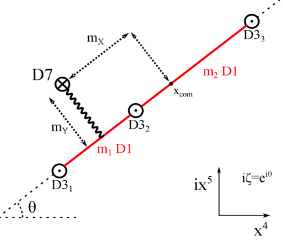
Figure 1: This figure illustrates the D-brane configuration corresponding to an SU(3) gauge theory with BPS monopoles of total magnetic charge $\gamma_{m}=m_{1}H_{\alpha_{1}}+m_{2}H_{\alpha_{2}}$ coupled to a single hypermultiplet in the fundamental representation with mass $\zeta^{-1}m=m_{y}+im_{x}$. Here have identified ${\mathbb{R}}_{x^{4}}\oplus{\mathbb{R}}_{x^{5}}\cong\mathbb{C}$ under $(x^{4},x^{5})\mapsto x^{4}+ix^{5}$. This figure shows that supersymmetric configurations of D3-branes must be collinear in $\mathbb{C}$, at an angle described by a phase $\zeta\in U(1)$, and that $m_{Y},m_{X}$ describe the displacement of the D7-brane from the center of mass of the D3-branes. Note that this is consistent with the definition of $\zeta^{-1}=-\frac{Z^{cl}}{|Z^{cl}|}$ as in (B.4).

Many aspects of magnetic monopole theory have beautiful geometrical interpretations in terms of D-brane configurations. Following the work of [7] we know that a system of monopoles in a d=4 N=2 SU(N) gauge theory can be realized by a system of N+1 parallel D3-branes with D1-branes stretched between them. We can then couple this theory to hypermultiplets by introducing D7-branes. This picture will give a geometric interpretation of the phase $\zeta$ and of the hypermultiplet mass parameters $m_{x}$ and $m_{y}$.

Consider a system of N+1 D3-branes where the $i^{th}$ brane (the D3_i-brane) is localized at $x^{6}=x^{7}=x^{8}=x^{9}=0$ and a fixed value $x^{4}+ix^{5}=v_{i}$ such that $v_{i}/v_{j}\in{\mathbb{R}}$ for all $v_{j}\neq 0$. These values, $v_{i}$, encode the expectation value of the adjoint valued scalar field in the d=4 N=2 SU(N) vectormultiplet. This tells us that the D3-branes form a straight line in the $x^{4}+ix^{5}$ plane whose angle is encoded by $\zeta$. The D1-branes are localized at points $(x^{1},x^{2},x^{3})=\vec{x}_{j}$ with $x^{6}=x^{7}=x^{8}=x^{9}=0$. The D1-branes are described in the effective theory of the D3-branes as magnetic monopoles located at $\vec{x}_{j}$. More accurately, they are D3-tubes running between the D3_i-branes.

We can now introduce hypermultiplets by adding D7-branes localized at definite values of $x^{4}+ix^{5}$, denoted by $m^{(v)}$. The strings stretching between the D7-branes and the D3-tubes support hypermultiplet fields. As such the length of these strings determine the mass of the lowest energy excitations. However, when there are multiple monopoles stretching between the nearest pair of D3-branes there are correspondingly many lowest energy excitations. These count the number of hypermultiplet zero modes and hence the index of the Dirac operator $L$ coupled to the mass $m_{X}=$Re$[\zeta^{-1}m^{(v)}]={\rm i}m_{x}$. The jumping of the index of the Dirac operator due to this coupling to $m_{X}$ implies that $m_{X}$ should be thought of as the displacement of the D7-brane along the line of D3-branes relative to the center of mass. Similarly $m_{Y}=$Im$[\zeta^{-1}m^{(v)}]=-{\rm i}m_{y}$ should be identified with the orthogonal distance of the D7-brane to the line of D3-branes. See Figure 1.

4 Application 1: Generalized Sen Conjecture

The discussion here is almost identical to section 4.1 of [20] so we will be extremely brief. Upon choosing a complex structure for ${\cal M}$ or $\overline{\underline{{\cal M}}}$ the bundles ${\cal E}_{\rm line}$ and ${\cal E}_{\rm matter}$ become holomorphic bundles with holomorphically flat connections, and hence the same holds for the bundle ${\cal E}$ defined in (8). The wavefunction describing the BPS state is an $L^{2}$ section of $\Lambda^{*}(T^{0,1}\overline{\underline{{\cal M}}})\otimes{\cal E}$, and a suitable combination of two collective coordinate supersymmetries is the Dolbeault operator

$$\bar{\partial}^{{\cal Y}}=\bar{\partial}_{{\cal E}}+\text{G}({\cal Y})^{0,1}\wedge\quad,$$ (20)

which squares to zero. The $SU(2)_{R}$ symmetry does not act on ${\cal E}$ because the hypermultiplet fermions are $SU(2)_{R}$ singlets and the line defect preserves $SU(2)_{R}$ symmetry. Hence the $SU(2)_{R}$ symmetry acts as a holomorphic Lefshetz $\mathfrak{s}\mathfrak{l}(2)$, exactly as in [20], equation (4.3). From the no-exotics theorem, conjectured in [13] and partially proven in [4, 5, 8], we learn that the $L^{2}$ cohomology of $\bar{\partial}^{{\cal Y}}$ is primitive and concentrated in the middle degree.

It is well-known that the (singular) monopole moduli space can be formulated, as a complex manifold, as a space of (meromorphic) maps from $\mathbb{C}\mathbb{P}^{1}$ to $G_{\mathbb{C}}/B$ where $G_{\mathbb{C}}$ is the complexification of $G$ and $B$ is a Borel subgroup. It is natural to formulate the line and matter holomorphic bundles in these terms, especially when stating the generalized Sen conjecture. We expect to explain this on another occasion.

As an interesting special case we consider $G=SU(2)$ with a hypermultiplet in the adjoint representation of mass $m$, and we take the $m\to 0$ limit. We take $m_{y}=0$ and for sufficiently small $m_{x}$ the bundle does not jump. In this case we can identify ${\cal E}_{\rm matter}$ with the holomorphic tangent bundle. It then follows that BPS states can be described by the self-dual harmonic forms on moduli space and in this way we recover the renowned prediction of Ashoke Sen based on $S$-duality [22]. We have thus made good on the promise at the end of Section 4.1 of [20].

5 Application 2: Explicit Formulae For $L^{2}$-Indices On Some Monopole Moduli Spaces

It was shown in [13] that if a half-supersymmetric line defect is wrapped on a thermal circle when the theory is put on ${\mathbb{R}}^{3}\times S^{1}$ then the vev can be expanded as

$$\langle L\rangle=\sum_{\gamma\in\Gamma_{L}}{\overline{\underline{\Omega}}}(L;\gamma;u){\cal Y}_{\gamma}$$ (21)

where $\Gamma_{L}$ is a torsor for the IR charge lattice $\Gamma$ and ${\cal Y}_{\gamma}$ are (locally defined) “Darboux functions” of the vacuum of the theory on ${\mathbb{R}}^{3}\times S^{1}$. (That is, they are locally defined functions on Seiberg-Witten moduli space - the total space of the abelian variety fibration over the Coulomb branch given by special geometry.) The “Darboux functions” obey the twisted group law:

$${\cal Y}_{\gamma_{1}}{\cal Y}_{\gamma_{2}}=(-1)^{\llangle\gamma_{1},\gamma_{2}\rrangle}{\cal Y}_{\gamma_{1}+\gamma_{2}}$$ (22)

using the electric-magnetic inner product on $\Gamma$. In addition, one can “retwist” by $(-1)^{2I_{3}}$, where $I_{3}$ is a generator of $SU(2)_{R}$ to obtain:

$$\langle L\rangle^{\prime}=\sum_{\gamma\in\Gamma_{L}}{\overline{\underline{\Omega}}}(L;\gamma;u)^{\prime}\tilde{\cal Y}_{\gamma}$$ (23)

with retwisted Darboux functions

$$\tilde{\cal Y}_{\gamma_{1}}\tilde{\cal Y}_{\gamma_{2}}=\tilde{\cal Y}_{\gamma_{1}+\gamma_{2}}.$$ (24)

Given the no-exotics property, we interpret ${\overline{\underline{\Omega}}}(L;\gamma;u)^{\prime}$ as the dimension of the space of framed BPS states and ${\overline{\underline{\Omega}}}(L;\gamma;u)$ as the trace of $(-1)^{2J_{3}}$ over this space.

As an application of our general result for the semiclassical interpretation of ${\overline{\underline{\Omega}}}(L;\gamma;u)$ when general line defects are included we specialize to the $G=SU(2)$ theory with $N_{f}=0$ and with $P=0$ and $Q=\frac{\kappa}{2}\alpha$ where $\kappa$ is a positive integer. Recall that $\Lambda_{wt}=\frac{\alpha}{2}{\mathbb{Z}}$ and $\Lambda_{mw}=\frac{H_{\alpha}}{2}{\mathbb{Z}}$ so that, in the $SU(2)$ theory,

$$\Gamma_{L}=\frac{\kappa}{2}\alpha+\Gamma=\Gamma=2\Lambda_{mw}\oplus\Lambda_{wt}.$$ (25)

Then the supersymmetric Wilson line is

$$W_{\kappa/2}:=L_{\zeta}[0,\frac{\kappa}{2}\alpha]={\rm Tr}_{\kappa+1}\Biggl{(}P{\rm exp}\oint\left[A-Y\right]\Biggr{)}$$ (26)

where here and below the subscript on the trace indicates the dimension of an irreducible representation, and the adjoint scalar $Y$ is defined in equation (54) below.

Since this is a theory of class S the quantum vev $\langle L\rangle$ is given by the classical holonomy of a complex flat connection on the underlying UV curve $C$. (See [13], section 7.4. The flat connection on $C$ encodes the vacuum on ${\mathbb{R}}^{3}\times S^{1}$ and the holonomy is taken around a closed loop on $C$ encoding the line defect $L$.) Now, for any group element $h$ in $SL(2,\mathbb{C})$ the trace in the irreducible representation of dimension $\kappa+1$ is related to that in the fundamental representation by

$${\rm Tr}_{\kappa+1}(h)=U_{\kappa}\left(\frac{1}{2}{\rm Tr}_{2}(h)\right)$$ (27)

where $U_{n}$ is the Chebyshev polynomial of the second kind, satisfying:

$$U_{n}(\cos\theta)=\frac{\sin[(n+1)\theta]}{\sin\theta}.$$ (28)

Therefore:

$$\langle W_{\kappa/2}\rangle=U_{\kappa}\left(\frac{1}{2}\langle W_{1/2}\rangle\right).$$ (29)

Now equation (10.33) of [13] gives an explicit expression:

$$\langle W_{1/2}\rangle={\cal Y}_{\frac{1}{2}\alpha}+{\cal Y}_{-\frac{1}{2}\alpha}+{\cal Y}_{H_{\alpha}+\frac{1}{2}(2c+1)\alpha}$$ (30)

where $c\in{\mathbb{Z}}$ labels chambers separated by the “BPS walls” where framed BPS states jump, and we work in a semiclassical domain where ${\cal Y}_{H_{\alpha}}$ is exponentially small as the coupling goes to zero. (The dependence on chamber comes about from the value of $Y_{\infty}$, and from the lift of $\zeta$ to the universal cover of $U(1)$.) There is a parallel expression for $\langle W_{\kappa/2}\rangle^{\prime}$ with ${\cal Y}_{\gamma}\rightarrow\tilde{\cal Y}_{\gamma}$.

Since $U_{\kappa}(x)$ is a polymomial in $x$ it is, in principle, straightforward to expand (29) to compute $\langle W_{\kappa/2}\rangle$ as an expansion in ${\cal Y}_{\gamma}$ and thereby obtain ${\overline{\underline{\Omega}}}(W_{\kappa/2};\gamma;u)$. On the other hand, given the results of the present paper, for $u$ in the weak-coupling chambers we can interpret the framed degeneracies as characters of an $L^{2}$- kernel of a Dirac-like operator on ${\cal M}(\gamma_{m};{\cal X})$. We spell out the identification in detail as follows:

The Dirac operator acts on spinors on ${\cal M}(\gamma_{m};{\cal X})$ (with $\gamma_{m}=mH_{\alpha}$) coupled to the hyperholomorphic bundle ${\cal E}_{\rm line}$. The bundle ${\cal E}_{\rm line}$ in this case is just the universal bundle in the $(\kappa+1)$-dimensional irreducible representation of $SU(2)$, restricted to $\{\vec{x}\}\times{\cal M}(\gamma_{m};{\cal X})$ (for any fixed $\vec{x}$). If ${\cal Y}=0$ we use the standard Dirac operator; in general we add Clifford multiplication by $\not{{\mathrm{G}}}({\cal Y})$ as in equation (5).

Now suppose that $\gamma=mH_{\alpha}+\frac{n_{e}}{2}\alpha$. Then BPS states of this charge are located in the $\frac{n_{e}}{2}\alpha$-isotypical component of the kernel of the Dirac operator. This means that on ${\cal M}(\gamma_{m};{\cal X})$ the Lie derivative of the spinor under the hyperholomorphic vector field $\text{G}(H_{\alpha})$ acts as

$${\cal L}_{\text{G}(H_{\alpha})}\Psi=-{\rm i}n_{e}\Psi.$$ (31)

Now, ${\overline{\underline{\Omega}}}(W_{\kappa/2};\gamma;u)$ is the trace of $(-1)^{2J_{3}}$ in the $\frac{n_{e}}{2}\alpha$-isotypical component while the retwisted degeneracy ${\overline{\underline{\Omega}}}(W_{\kappa/2};\gamma;u)^{\prime}$ is just the dimension of that component.

Expanding the Chebyshev polynomial in power series and rearranging a little we find

$$\langle W_{\kappa/2}\rangle=\sum_{m=0}^{\kappa}\sum_{n_{e}}{\overline{\underline{\Omega}}}(W_{\kappa/2},\gamma=mH_{\alpha}+\frac{n_{e}}{2}\alpha;u){\cal Y}_{mH_{\alpha}+\frac{n_{e}}{2}\alpha}$$ (32)

where the sum over $n_{e}$ only includes integers with $n_{e}=\kappa{\rm mod}2$ in the range

$$2m-\kappa\leq(n_{e}-2mc)\leq\kappa$$ (33)

and

$${\overline{\underline{\Omega}}}(W_{\kappa/2},\gamma=mH_{\alpha}+\frac{n_{e}}{2}\alpha;u)=(-1)^{\kappa(m-\kappa)}\sum_{\ell\geq 0}(-1)^{\ell}\binom{\kappa-\ell}{\ell}\binom{\kappa-2\ell}{m}\binom{\kappa-2\ell-m}{N_{c}-\ell}$$ (34)

with

$$N_{c}:=\frac{\kappa-(n_{e}-2mc)}{2}=\frac{\kappa-n_{e}}{2}+mc.$$ (35)

Note that $N_{c}\in{\mathbb{Z}}$. In (34) the summands vanish unless

$$0\leq\ell\leq{\rm Min}[N_{c},\kappa-N_{c+1}].$$ (36)

We can similarly expand $U_{\kappa}\left(\frac{1}{2}\langle W_{\kappa/2}\rangle^{\prime}\right)$ using the retwisted Darboux functions $\tilde{\cal Y}_{\gamma}$ and we find:

$${\overline{\underline{\Omega}}}(W_{\kappa/2},\gamma=mH_{\alpha}+\frac{n_{e}}{2}\alpha;u)^{\prime}=(-1)^{m(\kappa-m)}{\overline{\underline{\Omega}}}_{\cal Y}(W_{\kappa/2},\gamma=mH_{\alpha}+\frac{n_{e}}{2}\alpha;u)$$ (37)

This has the interesting consequence that for fixed charge $\gamma$ all the BPS states are either fermionic or bosonic, the parity being determined by the parity of $m(\kappa-m)$.

In fact, it is possible to simplify (34) by recognizing it as a special value of a hypergeometric series leading to the elegant result for the framed BPS degeneracy in the chamber labeled by $c\in{\mathbb{Z}}$:

$${\overline{\underline{\Omega}}}(W_{\kappa/2},\gamma=mH_{\alpha}+\frac{n_{e}}{2}\alpha;u)^{\prime}=\binom{N_{c+1}}{m}\binom{\kappa-N_{c}}{m}.$$ (38)

For fixed $m$ and $c$ this is a polynomial in $\kappa$ of order $2m$, suggestive of an index theorem on the (noncompact) monopole moduli space of dimension $4m$.

5.1 Marginally Bound States: Remark On A Paper Of Tong And Wong

Framed BPS states in N=2 gauge theory in the presence of a Wilson line have been previously studied by Tong and Wong in [27]. These authors also point out that inclusion of Wilson lines leads to a modification of the relevant Dirac operator by coupling to a bundle with connection. However, the paper [27] raised a puzzle because there is a slight discrepancy between their equation $(4.10)$ and the results of [13]. In this subsection we explain that the source of the discrepancy can be traced to how one handles marginally bound states.

In our notation, equation $(4.10)$ of [27] can be written as

$${\overline{\underline{\Omega}}}(W_{\kappa/2},\gamma=H_{\alpha}+\frac{n_{e}}{2}\alpha)^{\prime}=\frac{1}{2}\sum_{\begin{subarray}{c}|s|\leq\kappa\\ s\in 2{\mathbb{Z}}+\kappa\end{subarray}}s\text{ sign}(s-n_{e}-n_{e}\epsilon)$$ (39)

where $n_{e}\in 2{\mathbb{Z}}+\kappa$ and $\epsilon>0$ is an infinitesimal regularizing parameter. One way to obtain an analogous result from our expressions is to write

$$\langle W_{1/2}\rangle^{\prime}=\xi+\xi^{-1}$$ (40)

with

$$\xi=\frac{1}{2}\left(\tilde{\cal Y}_{\frac{1}{2}\alpha}+\tilde{\cal Y}_{-\frac{1}{2}\alpha}+\tilde{\cal Y}_{H_{\alpha}+\frac{1}{2}\alpha}+\sqrt{(\tilde{\cal Y}_{\frac{1}{2}\alpha}-\tilde{\cal Y}_{-\frac{1}{2}\alpha})^{2}+2(\tilde{\cal Y}_{\frac{1}{2}\alpha}+\tilde{\cal Y}_{-\frac{1}{2}\alpha})\tilde{\cal Y}_{H_{\alpha}+\frac{1}{2}\alpha}+\tilde{\cal Y}_{2H_{\alpha}+\alpha}}\right)$$ (41)

and then expand

$$\langle W_{\kappa/2}\rangle=\sum_{\begin{subarray}{c}s=-\kappa\\ s\in 2{\mathbb{Z}}+\kappa\end{subarray}}^{\kappa}\xi^{s}.$$ (42)

This gives, for example,

$$\begin{split}{\overline{\underline{\Omega}}}(W_{\kappa/2},\gamma=H_{\alpha}+\frac{n_{e}}{2}\alpha;u)^{\prime}&=\sum_{\begin{subarray}{c}s\geq|n_{e}|\\ s\in 2{\mathbb{Z}}+\kappa\end{subarray}}^{\kappa}s\Theta(s-1-|n_{e}-1|)\\ \end{split}$$ (43)

where $\Theta(x)\in\{0,1\}$ is the Heaviside step function and $\Theta(0)=1$. We can then rewrite this equation in a form analogous to (39):

$${\overline{\underline{\Omega}}}(W_{\kappa/2},\gamma=H_{\alpha}+\frac{n_{e}}{2}\alpha)^{\prime}=\frac{1}{2}\sum_{\begin{subarray}{c}|s|\leq\kappa\\ s\in 2{\mathbb{Z}}+\kappa\end{subarray}}s\text{ sign}(s-n_{e}\pm\epsilon)$$ (44)

where the choice of $\pm\epsilon$ is equivalent to choosing a chamber in which:

$$\langle W_{\frac{1}{2}}\rangle={\cal Y}_{\frac{1}{2}\alpha}\oplus{\cal Y}_{-\frac{1}{2}\alpha}+{\cal Y}_{H_{\alpha}\pm\frac{1}{2}\alpha}.$$ (45)

In [27] the framed BPS states with magnetic charge $m=1$ are counted via an index theorem, but the relevant Dirac operator is not Fredholm. The Dirac operator is evaluated for the theory at a wall of marginal stability. Physically, as explained in [27], one must worry about whether or not to include marginally bound states. The expression (39) makes use of one perturbation to a Fredholm operator. However the result conflicts with the general computation of (43) and (38) and hence the counting of boundstates used in [27] differs from that used in [13]. Another way to perturb to a Fredholm operator is to turn on a small generic ${\cal Y}$. This changes the perturbation, $n_{e}\to n_{e}+\epsilon n_{e}$, used in (39), to the perturbation $n_{e}\to n_{e}\mp\epsilon$, used in (44). The latter perturbation brings the index into line with the general results of [13].

Appendix A Review: The Universal Bundle And The Universal Connection

In this section we review the universal bundle of Atiyah and Singer [2]. (An expository account can be found in many places, among them [6] sec. 8.8.)

Let $G$ be a compact, semisimple Lie group with a trivial center and let $\pi:\mathfrak{P}\to M$ be a principal $G$ bundle and let $\mathcal{G}=\{\Phi:\mathfrak{P}\to\mathfrak{P}|\pi\circ\Phi=\pi\}$ be the group of gauge transformations (bundle automorphisms). Let ${\cal A}$ be the space of suitably smooth connections on $\mathfrak{P}$. The group $\mathcal{G}$ acts on $\mathfrak{P}\times\mathcal{A}$ by:

$$\begin{split}(p,A)\cdot g=(p\cdot g,g^{-1}Ag+g^{-1}dg)\hskip 28.45274pt\hskip 14.22636pt(p,A)\in\mathfrak{P}\times\mathcal{A}\end{split}$$ (46)

(Where $p\cdot g$ means the right-action on the principal $G$ bundle by the value of the gauge transformation $g$ at the point $\pi(p)\in M$.) We would like to form the $G\times{\cal G}$ bundle $\pi:\mathfrak{P}\times{\cal A}\to M\times{\cal A}/{\cal G}$ but because the group action can fail to be free we replace ${\cal A}$ by a space ${\cal A}^{*}$ whose raison d’etre is to have a free action.

Note that we have the diagram of projections:

$$\begin{split}\lx@xy@svg{\hbox{\raise 0.0pt\hbox{\kern 31.03197pt\hbox{\ignorespaces\ignorespaces\ignorespaces\hbox{\vtop{\kern 0.0pt\offinterlineskip\halign{\entry@#!@&&\entry@@#!@\cr&&\\&&\\&&\crcr}}}\ignorespaces{\hbox{\kern-3.0pt\raise 0.0pt\hbox{\hbox{\kern 0.0pt\raise 0.0pt\hbox{\hbox{\kern 3.0pt\raise 0.0pt\hbox{$\textstyle{}$}}}}}}}{\hbox{\kern 46.55971pt\raise 0.0pt\hbox{\hbox{\kern 0.0pt\raise 0.0pt\hbox{\hbox{\kern 3.0pt\raise 0.0pt\hbox{$\textstyle{\mathfrak{P}\times\mathcal{A}^{*}\ignorespaces\ignorespaces\ignorespaces\ignorespaces\ignorespaces\ignorespaces\ignorespaces\ignorespaces}$}}}}}}}\ignorespaces\ignorespaces\ignorespaces{}\ignorespaces\ignorespaces{\hbox{\lx@xy@drawline@}}\ignorespaces\ignorespaces\ignorespaces{\hbox{\kern 86.14116pt\raise-16.73608pt\hbox{{}\hbox{\kern 0.0pt\raise 0.0pt\hbox{\hbox{\kern 3.0pt\hbox{\hbox{\kern 0.0pt\raise-2.39166pt\hbox{$\scriptstyle{G}$}}}\kern 3.0pt}}}}}}\ignorespaces{\hbox{\kern 99.0647pt\raise-33.1194pt\hbox{\hbox{\kern 0.0pt\raise 0.0pt\hbox{\lx@xy@tip{1}\lx@xy@tip{-1}}}}}}\ignorespaces\ignorespaces{\hbox{\lx@xy@drawline@}}\ignorespaces{\hbox{\lx@xy@drawline@}}\ignorespaces\ignorespaces\ignorespaces{}\ignorespaces\ignorespaces{\hbox{\lx@xy@drawline@}}\ignorespaces\ignorespaces\ignorespaces{\hbox{\kern 21.14632pt\raise-16.73608pt\hbox{{}\hbox{\kern 0.0pt\raise 0.0pt\hbox{\hbox{\kern 3.0pt\hbox{\hbox{\kern 0.0pt\raise-2.39166pt\hbox{$\scriptstyle{{\cal G}}$}}}\kern 3.0pt}}}}}}\ignorespaces{\hbox{\kern 15.60574pt\raise-33.1194pt\hbox{\hbox{\kern 0.0pt\raise 0.0pt\hbox{\lx@xy@tip{1}\lx@xy@tip{-1}}}}}}\ignorespaces\ignorespaces{\hbox{\lx@xy@drawline@}}\ignorespaces{\hbox{\lx@xy@drawline@}}{\hbox{\kern 108.51666pt\raise 0.0pt\hbox{\hbox{\kern 0.0pt\raise 0.0pt\hbox{\hbox{\kern 3.0pt\raise 0.0pt\hbox{$\textstyle{}$}}}}}}}{\hbox{\kern-31.03197pt\raise-44.2555pt\hbox{\hbox{\kern 0.0pt\raise 0.0pt\hbox{\hbox{\kern 3.0pt\raise 0.0pt\hbox{$\textstyle{{\cal Q}=\mathfrak{P}\times\mathcal{A}^{*}/\mathcal{G}\ignorespaces\ignorespaces\ignorespaces\ignorespaces}$}}}}}}}\ignorespaces\ignorespaces\ignorespaces{}\ignorespaces\ignorespaces{\hbox{\lx@xy@drawline@}}\ignorespaces\ignorespaces\ignorespaces{\hbox{\kern 21.05852pt\raise-72.19156pt\hbox{{}\hbox{\kern 0.0pt\raise 0.0pt\hbox{\hbox{\kern 3.0pt\hbox{\hbox{\kern 0.0pt\raise-2.39166pt\hbox{$\scriptstyle{G}$}}}\kern 3.0pt}}}}}}\ignorespaces{\hbox{\kern 46.70016pt\raise-78.20822pt\hbox{\hbox{\kern 0.0pt\raise 0.0pt\hbox{\lx@xy@tip{1}\lx@xy@tip{-1}}}}}}\ignorespaces\ignorespaces{\hbox{\lx@xy@drawline@}}\ignorespaces{\hbox{\lx@xy@drawline@}}{\hbox{\kern 59.0014pt\raise-44.2555pt\hbox{\hbox{\kern 0.0pt\raise 0.0pt\hbox{\hbox{\kern 3.0pt\raise 0.0pt\hbox{$\textstyle{}$}}}}}}}{\hbox{\kern 92.97084pt\raise-44.2555pt\hbox{\hbox{\kern 0.0pt\raise 0.0pt\hbox{\hbox{\kern 3.0pt\raise 0.0pt\hbox{$\textstyle{M\times\mathcal{A}^{*}\ignorespaces\ignorespaces\ignorespaces\ignorespaces}$}}}}}}}\ignorespaces\ignorespaces\ignorespaces{}\ignorespaces\ignorespaces{\hbox{\lx@xy@drawline@}}\ignorespaces\ignorespaces\ignorespaces{\hbox{\kern 86.24275pt\raise-72.19156pt\hbox{{}\hbox{\kern 0.0pt\raise 0.0pt\hbox{\hbox{\kern 3.0pt\hbox{\hbox{\kern 0.0pt\raise-2.39166pt\hbox{$\scriptstyle{{\cal G}}$}}}\kern 3.0pt}}}}}}\ignorespaces{\hbox{\kern 74.23587pt\raise-78.20822pt\hbox{\hbox{\kern 0.0pt\raise 0.0pt\hbox{\lx@xy@tip{1}\lx@xy@tip{-1}}}}}}\ignorespaces\ignorespaces{\hbox{\lx@xy@drawline@}}\ignorespaces{\hbox{\lx@xy@drawline@}}{\hbox{\kern-3.0pt\raise-89.34431pt\hbox{\hbox{\kern 0.0pt\raise 0.0pt\hbox{\hbox{\kern 3.0pt\raise 0.0pt\hbox{$\textstyle{}$}}}}}}}{\hbox{\kern 37.03197pt\raise-89.34431pt\hbox{\hbox{\kern 0.0pt\raise 0.0pt\hbox{\hbox{\kern 3.0pt\raise 0.0pt\hbox{$\textstyle{M\times\mathcal{A}^{*}/\mathcal{G}}$}}}}}}}{\hbox{\kern 108.51666pt\raise-89.34431pt\hbox{\hbox{\kern 0.0pt\raise 0.0pt\hbox{\hbox{\kern 3.0pt\raise 0.0pt\hbox{$\textstyle{}$}}}}}}}\ignorespaces}}}}\ignorespaces\end{split} \textstyle{\mathfrak{P}\times\mathcal{A}^{*}\ignorespaces\ignorespaces\ignorespaces\ignorespaces\ignorespaces\ignorespaces\ignorespaces\ignorespaces} \scriptstyle{G} \scriptstyle{{\cal G}} \textstyle{{\cal Q}=\mathfrak{P}\times\mathcal{A}^{*}/\mathcal{G}\ignorespaces\ignorespaces\ignorespaces\ignorespaces} \scriptstyle{G} \textstyle{M\times\mathcal{A}^{*}\ignorespaces\ignorespaces\ignorespaces\ignorespaces} \scriptstyle{{\cal G}} \textstyle{M\times\mathcal{A}^{*}/\mathcal{G}} \textstyle{\mathfrak{P}\times\mathcal{A}^{*}\ignorespaces\ignorespaces\ignorespaces\ignorespaces\ignorespaces\ignorespaces\ignorespaces\ignorespaces} \scriptstyle{G} \scriptstyle{{\cal G}} \textstyle{{\cal Q}=\mathfrak{P}\times\mathcal{A}^{*}/\mathcal{G}\ignorespaces\ignorespaces\ignorespaces\ignorespaces} \scriptstyle{G} \textstyle{M\times\mathcal{A}^{*}\ignorespaces\ignorespaces\ignorespaces\ignorespaces} \scriptstyle{{\cal G}} \textstyle{M\times\mathcal{A}^{*}/\mathcal{G}}$$ (47)

The principal $G$-bundle $\pi:{\cal Q}\to M\times\mathcal{A}^{*}/\mathcal{G}$ was referred to by Atiyah and Singer as the universal bundle, (and indeed it enjoys a universal property). Another useful bundle is the principal $G\times{\cal G}$-bundle with total space $\mathfrak{Q}:=\mathfrak{P}\times{\cal A}^{*}$ and projection $\pi:\mathfrak{Q}\to M\times{\cal A}^{*}/{\cal G}$.

The bundle $\mathfrak{Q}$ has a natural connection which we will refer to (by a slight abuse of terminology) as the universal connection. To define it, note that, given a metric on $M$ and a Killing metric ${\rm Tr}(...)$ on $\mathfrak{g}$ there is a natural metric on ${\cal A}$ defined by

$$(\tau_{1},\tau_{2})=\int_{M}{\rm vol\,}{\rm Tr}(\tau_{1}*\tau_{2})$$ (48)

where $\tau_{i}\in T_{A}{\cal A}\cong\Omega^{1}(M;{\rm ad}(\mathfrak{P}))$, with $i=1,2$. Now, a connection can be defined by specifying the horizontal subspaces of $\mathfrak{Q}$ in the tangent space $T_{p,A}\mathfrak{Q}\cong T_{p}\mathfrak{P}\oplus T_{A}{\cal A}$ orthogonal to the subspace of vertical vectors $\cong\mathfrak{g}\oplus{\rm Lie}({\cal G})$. The horizontal subspace is defined by

$$H_{p,A}:=H_{p}(A)\oplus{\rm Lie}({\cal G})^{\perp}$$ (49)

where $H_{p}(A)\subset T_{p}\mathfrak{P}$ is the horizontal subspace determined by the connection $A$ and ${\rm Lie}({\cal G})^{\perp}$ is the orthogonal complement to the infinitesimal gauge transformations in the metric (48).

Note that a very similar construction also gives a connection on $\pi:{\cal A}^{*}\to{\cal A}^{*}/{\cal G}$, namely, the horizontal subspaces are the orthogonal subspaces to the gauge orbits in the metric (48). By an even more abusive use of terminology we will also refer to this connection as the “universal connection.” It will be useful to be more explicit about this connection: If $\tau=\frac{d}{dt}A(t)$ is a tangent vector at $A\in{\cal A}^{*}$ then since the vertical vector fields in $T_{A}{\cal A}^{*}$ are associated to $\epsilon:M\to\Omega^{0}(M;{\rm ad}(\mathfrak{P}))$ and given by $\tau_{\epsilon}:=-D_{A}\epsilon$ the horizontal projection of $\tau$ is

$$H(\tau)=\tau-D_{A}\tilde{\epsilon}$$ (50)

where $\tilde{\epsilon}$ is the unique solution to $D_{A}*(\tau-D_{A}\tilde{\epsilon})=0$ vanishing at the framing point $x_{0}$.

In the application to magnetic monopoles we take $M={\mathbb{R}}^{3}$ with Euclidean metric and choose $x_{0}$ to be a point at infinity (chosen along a particular direction). The “connections” in ${\cal A}$ are actually translationally invariant connections $\hat{A}$ on $M\times{\mathbb{R}}$, and we interpret

$$\hat{A}=A_{i}dx^{i}+Xdx^{4}$$ (51)

where $X$ is the Higgs field valued in $\mathfrak{g}$. One often pulls back the bundle to ${\cal M}\subset{\cal A}^{*}/{\cal G}$. In this context, if $\hat{A}(z^{m})$ is a family of gauge-inequivalent solutions to the Bogomolnyi equations parametrized by an open set of ${\cal M}$ with local coordinates $z^{m}$, $m=1,\dots,{\rm dim}_{{\mathbb{R}}}{\cal M}$ then

$$\tau_{m}=\frac{\partial\hat{A}}{\partial z^{m}}$$ (52)

is in general not in the horizontal subspace and the compensating gauge transformation $\tilde{\epsilon}$ defined above is denoted $\epsilon_{m}$, with horizontal projection $H(\tau_{m}):=\delta_{m}\hat{A}$. This defines notation used in equation (19) above and in appendix B below.

Finally, in the case of singular monopoles, the connection $\hat{A}=(A,X)$ must satisfy the boundary conditions (59) at the location of each line defect $\vec{x}_{j}$. As explained carefully in [14, 21] this means there is a reduction of structure group at $\{\vec{x}_{j}\}\times{\cal A}^{*}/{\cal G}$ to $Z(P_{j})\subset G$, the centralizer of the ’t Hooft charge at $\vec{x}_{j}$. Note that if $P=0$ then $Z(P)=G$.

Appendix B Proof Using Supersymmetric Quantum Mechanics

In this appendix we provide a few of the details of the formulation of the collective coordinate supersymmetric quantum mechanics which is the basis of the above formulation of the semiclassical space of BPS states.

The UV Lagrangian written in d=4 N=1 superspace is (using standard notation, such as in [16]):

$$\begin{split}\mathcal{L}=&\left[-\frac{{\rm i}\tau}{4\pi}\int d^{2}\theta{\rm Tr}(W_{\alpha}W^{\alpha})+c.c.\right]+\frac{\text{Im }\tau}{4\pi}\int d^{4}\theta\text{ }\Phi^{\dagger}e^{2iV}\Phi\\ &+\frac{\text{Im }\tau}{4\pi}\left\{\int d^{4}\theta\left(Q^{\dagger}e^{2iV}Q+\tilde{Q}^{\dagger}e^{-2iV}\tilde{Q}\right)+\left[\int d^{2}\theta(i\tilde{Q}\Phi Q+i\tilde{Q}mQ)+c.c.\right]\right\}\end{split}$$ (53)

Here we have assumed $G$ is a simple group and $W_{\alpha}$ is the chiral superfield associated to an $N=1$ vectormultiplet for $G$, while $\Phi$ is a chiral superfield in the adjoint of $G$. Note that the N=1 superspace formalism implicitly assumes a splitting of the quaternionic representation of $G_{f}\times G$ in the form ${\cal R}=\rho\oplus\rho^{\ast}$ with chiral superfields $Q$ and $\tilde{Q}$ transforming in representations $\rho$ and $\rho^{*}$, respectively. Finally, without loss of generality we can assume $m\in\mathfrak{t}_{f}\otimes\mathbb{C}$.

We next write out the Lagrangian in terms of the components of the superfields. The lowest component of $\Phi$ is the scalar $\varphi$ valued in $\mathfrak{g}\otimes\mathbb{C}$. It is convenient to decompose the vectormultiplet scalar fields and mass parameters into “real” and “imaginary” parts according to

$$\zeta^{-1}\varphi=Y+{\rm i}X\qquad Y,X\in\mathfrak{g}$$ (54)

$$\zeta^{-1}m=m_{y}+{\rm i}m_{x}\qquad m_{y},m_{x}\in\mathfrak{t}_{f}.$$ (55)

As noted above, $\zeta$ will be the phase defining the line defect, or, if there is no line defect, it is the phase of the classical limit of the central charge

$$\zeta^{-1}=-\frac{Z^{cl}}{|Z^{cl}|}\qquad Z^{cl}=\frac{4\pi{\rm i}}{g_{0}^{2}}(Y_{\infty}+{\rm i}X_{\infty},\gamma_{m})$$ (56)

where $X_{\infty}$ and $Y_{\infty}$ are vacuum expectation values of $X,Y$ at $\vec{x}\to\infty$. That is, we have boundary conditions at infinity:

$$\begin{split}X&=X_{\infty}-\frac{\gamma_{m}}{2r}+\cdots\\ F&=\frac{1}{2}\gamma_{m}\omega+\cdots\\ \end{split}$$ (57)

and $Y\to Y_{\infty}+\cdots$ (compatible with the equations of motion) to leading order in a large $r$ expansion. The vevs $X_{\infty},Y_{\infty}$ are related to the vevs ${\cal X},{\cal Y}$ used elsewhere in this note by:

$${\cal X}=X_{\infty}\hskip 28.45274pt{\cal Y}=\frac{4\pi}{g_{0}^{2}}Y_{\infty}+\frac{\theta_{0}}{2\pi}X_{\infty}.$$ (58)

If we use the definitions (4) then these are only the leading expressions in a weak coupling expansion. (It was argued in [21] that the higher order terms in the definition (4) correctly capture perturbative corrections to the collective coordinate dynamics.)

The ’t Hooft-Wilson operator $L_{\zeta}[P_{j},Q_{j}]$, inserted at a point $\vec{x}_{j}$ modifies the path integral in two ways:

1. First, it modifies the boundary conditions on the fields over which we integrate. We choose a representative of $[P_{j},Q_{j}]$ so that $Q_{j}$ is a dominant weight of $Z(P_{j})$ and impose boundary conditions near $\vec{x}_{j}$:

   $$\begin{split}B^{i}&=\frac{P_{j}}{2r_{j}^{2}}\hat{r}_{j}^{i}+O(r_{j}^{-3/2})\hskip 28.45274ptE^{i}=\frac{g_{0}^{2}}{4\pi}\frac{Q_{j}^{\ast}}{2r_{j}^{2}}\hat{r}_{j}^{i}-\frac{\tilde{\theta}_{0}P_{j}}{2r_{j}^{2}}\hat{r}_{j}^{i}+O(r^{-3/2})\\ X&=-\frac{P_{j}}{2r_{j}}+O(r_{j}^{-1/2})\hskip 31.29802ptY=-\frac{g_{0}^{2}}{4\pi}\frac{Q_{j}^{\ast}}{2r_{j}}+\frac{\tilde{\theta}_{0}P_{j}}{2r_{j}}+O(r_{j}^{-1/2})\end{split}$$ (59)

   where $r_{j}=|\vec{x}-\vec{x}_{j}|$, $Q_{j}\in\Lambda_{wt}$ is the highest weight of a representation $R_{j}$ of $Z(P_{j})$, and $Q_{j}^{\ast}\in\mathfrak{t}$ is the dual of $Q_{j}$ under the canonical pairing $\langle$ , $\rangle:\mathfrak{t}^{\vee}\times\mathfrak{t}\to{\mathbb{R}}$.

2. Second, we insert a quantum mechanical path integral, representing modes located at the position of the line defect. Let $R_{j}\cong\mathbb{C}^{N_{j}}$ denote the irreducible representation with highest weight $Q_{j}$. We may assume it is a unitary representation with the standard Hermitian metric. We introduce $N_{j}$ complex fermions $w_{j}\in R_{j}$ and introduce the action

   $$S_{j}=\int d^{4}x\text{ }\delta^{(3)}(x-x_{j})\left[iw_{j}^{\dagger}\left(\partial_{t}+R_{j}(A_{0}-Y)-{\rm i}\alpha_{j}(t)\right)w_{j}+\frac{N-2}{2}\alpha_{j}(t)\right]$$ (60)

   Here and below we use the notation $R_{j}(F)$ to indicate that a $\mathfrak{g}$-valued field $F$ is evaluated at $\vec{x}_{j}$ and then represented in the $R_{j}$ representation. We are again using the notation for $R_{j}$ in a way similar to that explained in the footnote under equation (19). In equation (60) note that the pole structure of $A_{0}$ and $Y$ do not always allow them to be defined at the the points $\vec{x}_{j}$, but their difference will always be well defined. Finally, $\alpha_{j}(t)$ is a Lagrangian multiplier enforcing the constraint that in the Hilbert space we project onto the one-particle sector for the number operator

   $$\frac{1}{2}(w_{j}^{\dagger}w_{j}-w_{j}w_{j}^{\dagger}).$$ (61)

We now introduce collective coordinates. We choose a local patch in ${\cal M}$ or $\overline{\underline{{\cal M}}}$ with coordinates $z^{m}$, $m=1\dots,{\rm dim}_{{\mathbb{R}}}{\cal M}$ or ${\rm dim}_{{\mathbb{R}}}\overline{\underline{{\cal M}}}$ and promote these to time-dependent fields. Then we try to solve the classical equations of motion. The solution of the Dirac equation for the vectormultiplet fermions introduces superpartners $\chi^{m}(t)$. When we include the hypermultiplets the hypermultiplet scalars are set to zero (for generic point on the Coulomb branch, and certainly in the semiclassical limit where $u\to\infty$) and the solution of the Dirac equation for the hypermultiplet fermions introduces real fermionic coordinates $\psi^{s}(t)$ with $s=1,\dots,{\rm dim}_{{\mathbb{R}}}{\cal E}_{\rm matter}$.

The result of a fairly long computation is the collective coordinate Lagrangian:

$$\begin{split}L_{c.c.}&=\frac{4\pi}{g_{0}^{2}}\left[\frac{1}{2}g_{mn}\left(\dot{z}^{m}\dot{z}^{n}+{\rm i}\chi^{m}\mathcal{D}_{t}\chi^{n}-\text{G}(Y_{\infty})^{m}\text{G}(Y_{\infty})^{n}\right)+\frac{{\rm i}}{2}\chi^{m}\chi^{n}\nabla_{m}\text{G}(Y_{\infty})_{n}\right]\\ &-\frac{4\pi}{g_{0}^{2}}\left[{\rm i}h_{ss^{\prime}}\psi^{s}\mathcal{D}_{t}\psi^{s^{\prime}}-{\rm i}\psi^{s}(m_{y,ss^{\prime}}+T_{ss^{\prime}})\psi^{s^{\prime}}+\frac{1}{2}F_{mn,ss^{\prime}}\chi^{m}\chi^{n}\psi^{s}\psi^{s^{\prime}}\right]\\ &-\frac{4\pi}{g_{0}^{2}}(\gamma_{m},X_{\infty})+\frac{\theta_{0}}{2\pi}(\gamma_{m},Y_{\infty})+\frac{\theta_{0}}{2\pi}\Big{(}g_{mn}(\dot{z}^{m}-\text{G}(X_{\infty})^{m})\text{G}(Y_{\infty})^{n}-{\rm i}\chi^{m}\chi^{n}\nabla_{m}\text{G}(X_{\infty})_{n}\Big{)}\\ &+{\rm i}\sum_{j}w^{\dagger}_{j}(\partial_{t}+R_{j}(\epsilon_{Y_{\infty}})-R_{j}(\epsilon_{m})\dot{z}^{m}+\frac{{\rm i}}{2}R_{j}(\phi_{mn})\chi^{m}\chi^{n}-{\rm i}\alpha_{j}(t))w_{j}+\frac{N-2}{2}\alpha_{j}(t)\end{split}$$ (62)

Here $\epsilon_{m}$ is the compensating gauge transformation used in defining the universal connection, as defined under (52). The corresponding curvature of the universal connection is

$$\phi_{mn}=[D_{m},D_{n}]$$ (63)

where $D_{m}=\frac{\partial}{\partial z^{m}}+[\epsilon_{m},\cdot]$. Similarly, for any element $H\in\mathfrak{t}$ we define $\epsilon_{H}$ to be the solution of $\hat{D}^{2}\epsilon_{H}=0$ with boundary condition that $\epsilon_{H}\to H$ at infinity. In addition we have:

$$g_{mn}=\frac{1}{2\pi}\int_{\mathbb{R}^{3}}d^{3}x\text{ Tr}\left\{\delta_{m}\hat{A}^{a}\delta_{n}\hat{A}_{a}\right\}\hskip 28.45274pt\Gamma_{mnp}=\frac{1}{2\pi}\int_{\mathbb{R}^{3}}d^{3}x\text{ Tr}\left\{\delta_{m}\hat{A}^{a}D_{p}\delta_{n}\hat{A}_{a}\right\}$$

$$\mathcal{D}_{t}\chi^{n}=\dot{\chi}^{n}+\Gamma^{n}_{mp}\dot{z}^{m}\chi^{p}\hskip 28.45274pt\mathcal{D}_{t}\psi^{s}=\dot{\psi}^{s}+\dot{z}^{m}(A_{m})^{s}_{\text{ }s^{\prime}}\psi^{s^{\prime}}$$

$$m_{y,ss^{\prime}}=\frac{1}{2\pi}\int d^{3}x\text{ }\overline{\lambda}_{s}m_{y}\lambda_{s^{\prime}}\hskip 65.44133ptA_{m,ss^{\prime}}=\frac{1}{2\pi}\int d^{3}x\text{ }\overline{\lambda}_{s}(\partial_{m}+{\cal R}(\epsilon_{m}))\lambda_{s^{\prime}}$$

$$T_{ss^{\prime}}=\frac{1}{2\pi}\int d^{3}x\text{ }\overline{\lambda}_{s}{\cal R}(\epsilon_{Y_{\infty}})\lambda_{s^{\prime}}\hskip 28.45274ptF_{mn,ss^{\prime}}=\partial_{m}A_{n,ss^{\prime}}-\partial_{n}A_{m,ss^{\prime}}+(A_{m}A_{n}-A_{n}A_{m})_{ss^{\prime}}$$

One can check that the action is invariant under the $N=4$ supersymmetry transformations:

$$\begin{split}\delta_{\nu}z^{m}&=-{\rm i}\nu_{a}(\tilde{\mathbb{J}}^{a})^{m}_{\text{ }n}\chi^{n}\\ \delta_{\nu}\chi^{m}&=(\mathbb{J}^{a})^{m}_{\text{ }n}(\dot{z}^{n}-\text{G}(Y_{\infty})^{n})\nu_{a}-{\rm i}\nu_{a}\chi^{k}\chi^{n}(\mathbb{J}^{a})_{k}^{\ell}\Gamma_{\ell n}^{m}\\ \delta_{\nu}\psi^{s}&=-A_{m,s^{\prime}}^{s}\delta_{\nu}z^{m}\psi^{s^{\prime}}\\ \delta_{\nu}w_{j}&=\delta_{\nu}z^{m}R_{j}(\epsilon_{m})w_{j}\\ \delta_{\nu}\alpha_{j}(t)&=0\end{split}$$ (64)

where

$$\begin{split}\mathbb{J}^{a}=(\mathbb{J}^{r},\textbf{1})\hskip 28.45274pt\tilde{\mathbb{J}}^{a}=(-\mathbb{J}^{r},\textbf{1})\end{split}$$ (65)

for an index $a=1,2,3,4$ and where $\mathbb{J}^{r}$, $r=1,2,3$ are three covariantly constant complex structures on $\overline{\underline{{\cal M}}}$ (or ${\cal M}$) satisfying the quaternion relations. Note that the number operator for the $w_{j}$ fermions is invariant under supersymmetry transformations so we may restrict to the one-particle sector without breaking supersymmetry. The check that the action is indeed invariant under (64) makes use of the property that the connections on ${\cal E}_{\rm matter}$ and ${\cal E}_{\rm line}$ are hyperholomorphic. Because the collective coordinate Lagrangian must have N=4 supersymmetry this can be regarded as a proof that these connections are indeed hyperholomorphic.

Upon quantization we find the supercharge operators:

$$\begin{split}\hat{Q}^{a}&=-\frac{{\rm i}g_{0}}{2\sqrt{2\pi}}\gamma^{m}(\tilde{\mathbb{J}}^{a})_{m}^{\text{ }n}\times\\ &\left(\partial_{m}+\frac{1}{4}\omega_{m,pq}\gamma^{pq}+\frac{1}{2}\Omega_{m,ss^{\prime}}\theta^{ss^{\prime}}-\sum_{j}w_{j}^{\dagger}R_{j}(\epsilon_{m}^{(j)})w_{j}-{\rm i}\text{G}({\cal Y}_{\infty})_{m}\right)\end{split}$$ (66)

where $\omega_{m,pq}$ is the spin connection for the hyperkähler  metric on the monopole moduli space $\Omega_{m,ss^{\prime}}$ is the hyperholomorphic connection on ${\cal E}_{\rm matter}$ and $\theta^{s}$ are the gamma matrices acting on ${\rm Spin}({\cal E}_{\rm matter})$ so that $\theta^{ss^{\prime}}:=\theta^{s}\theta^{s^{\prime}}$ for $s\not=s^{\prime}$.

One can check - as expected - that these operators satisfy the N=4 SQM algebra:

$$\{\hat{Q}^{a},\hat{Q}^{b}\}=2\delta^{ab}(\hat{H}-\text{Re}(\zeta^{-1}\hat{Z}))$$ (67)

The central charge satisfies:

$$\text{Re}(\zeta^{-1}\hat{Z})=M_{\gamma}^{1-lp}$$ (68)

where

$$\hat{Z}=(\gamma_{m},a_{D})+\hat{\gamma}_{e}\cdot a+\hat{\gamma}_{f}\cdot m$$ (69)

and $\hat{\gamma}_{e}$ and $\hat{\gamma}_{f}$ are operators in the quantum mechanics. The operator $\hat{\gamma}_{e}$ is defined by the generators of the global gauge transformations in $T$ (see [21] for the detailed expressions) while

$$\hat{\gamma}_{f}\cdot m_{y}=i\theta^{s}m_{y,ss^{\prime}}\theta^{s^{\prime}}.$$ (70)

When representing the Clifford algebra $\theta^{s}$ we must choose a proper normal-ordering constant, and this must be determined by physical considerations. For example, in the string theory interpretation of section 3.3 it should represent the energy from the tension of fundamental strings stretched between the D7 and D3 branes.

It follows from the supersymmetry algebra that a wavefunction is in the kernel of $\hat{Q}^{a}$ either for all operators $a=1,2,3,4$ of for none of them. Therefore, it suffices to focus on the Dirac operator proportional to $\hat{Q}^{4}$:

$${\rm i}\gamma^{m}\left(\partial_{m}+\frac{1}{4}\omega_{m,pq}\gamma^{pq}+\frac{1}{2}\Omega_{m,ss^{\prime}}\theta^{ss^{\prime}}-\sum_{j}w_{j}^{\dagger}R_{j}(\epsilon_{m})w_{j}-{\rm i}\text{G}({\cal Y})_{m}\right)$$ (71)

The BPS states with magnetic charge $\gamma_{m}$ are the $L^{2}$ wavefunctions on ${\cal M}$ or $\overline{\underline{{\cal M}}}$ in the kernel of $\hat{Q}^{4}$. The subspaces with definite electric and flavor charge are the isotypical subspaces of the $T_{f}\times T$ action on the kernel - equivalently - the eigenspaces of $\hat{\gamma}_{e}$ and $\hat{\gamma}_{f}$.

References

• [1] P. C. Argyres, M. R. Plesser and N. Seiberg, “The Moduli space of vacua of N=2 SUSY QCD and duality in N=1 SUSY QCD,” Nucl. Phys. B 471, 159 (1996) doi:10.1016/0550-3213(96)00210-6 [hep-th/9603042].
• [2] M. F. Atiyah and I. M. Singer, “Dirac Operators Coupled to Vector Potentials,” Proc. Nat. Acad. Sci.  81, 2597 (1984). doi:10.1073/pnas.81.8.2597
• [3] C. Callias, “Index Theorems on Open Spaces,” Commun. Math. Phys.  62, 213 (1978). doi:10.1007/BF01202525
• [4] W. y. Chuang, D. E. Diaconescu, J. Manschot, G. W. Moore and Y. Soibelman, “Geometric engineering of (framed) BPS states,” Adv. Theor. Math. Phys.  18, no. 5, 1063 (2014) doi:10.4310/ATMP.2014.v18.n5.a3 [arXiv:1301.3065 [hep-th]].
• [5] C. Cordova and T. Dumitrescu. to Appear See Strings2016 talk by T. Dumitrescu. URL http://ymsc.tsinghua.edu.cn:8090/strings/?page_id=1024.
• [6] S. Cordes, G. W. Moore and S. Ramgoolam, “Lectures on 2-d Yang-Mills theory, equivariant cohomology and topological field theories,” Nucl. Phys. Proc. Suppl.  41, 184 (1995) doi:10.1016/0920-5632(95)00434-B [hep-th/9411210].
• [7] D. E. Diaconescu, “D-branes, monopoles and Nahm equations,” Nucl. Phys. B 503, 220 (1997) doi:10.1016/S0550-3213(97)00438-0 [hep-th/9608163].
• [8] M. Del Zotto and A. Sen, “About the Absence of Exotics and the Coulomb Branch Formula,” arXiv:1409.5442 [hep-th].
• [9] J. P. Gauntlett, “Low-energy dynamics of N=2 supersymmetric monopoles,” Nucl. Phys. B 411, 443 (1994) doi:10.1016/0550-3213(94)90457-X [hep-th/9305068].
• [10] J. P. Gauntlett and J. A. Harvey, “S duality and the dyon spectrum in N=2 superYang-Mills theory,” Nucl. Phys. B 463, 287 (1996) doi:10.1016/0550-3213(96)00035-1 [hep-th/9508156].
• [11] J. P. Gauntlett, N. Kim, J. Park and P. Yi, “Monopole dynamics and BPS dyons N=2 superYang-Mills theories,” Phys. Rev. D 61, 125012 (2000) [hep-th/9912082].
• [12] J. P. Gauntlett, C. j. Kim, K. M. Lee and P. Yi, “General low-energy dynamics of supersymmetric monopoles,” Phys. Rev. D 63, 065020 (2001) doi:10.1103/PhysRevD.63.065020 [hep-th/0008031].
• [13] D. Gaiotto, G. W. Moore and A. Neitzke, “Framed BPS States,” Adv. Theor. Math. Phys.  17, no. 2, 241 (2013) doi:10.4310/ATMP.2013.v17.n2.a1 [arXiv:1006.0146 [hep-th]].
• [14] A. Kapustin, “Wilson-’t Hooft operators in four-dimensional gauge theories and S-duality,” Phys. Rev. D 74, 025005 (2006) doi:10.1103/PhysRevD.74.025005 [hep-th/0501015].
• [15] A. Kapustin, “Holomorphic reduction of N=2 gauge theories, Wilson-’t Hooft operators, and S-duality,” hep-th/0612119.
• [16] J. Labastida and M. Marino, “Topological quantum field theory and four manifolds,” (Mathematical physics studies. 25)
• [17] N. S. Manton and B. J. Schroers, “Bundles over moduli spaces and the quantization of BPS monopoles,” Annals Phys.  225, 290 (1993). doi:10.1006/aphy.1993.1060
• [18] G. W. Moore, A. B. Royston and D. Van den Bleeken, “Parameter counting for singular monopoles on $\mathbb{R}^{3}$,” JHEP 1410, 142 (2014) doi:10.1007/JHEP10(2014)142 [arXiv:1404.5616 [hep-th]].
• [19] G. W. Moore, A. B. Royston and D. Van den Bleeken, “Brane bending and monopole moduli,” JHEP 1410, 157 (2014) doi:10.1007/JHEP10(2014)157 [arXiv:1404.7158 [hep-th]].
• [20] G. W. Moore, A. B. Royston and D. Van den Bleeken, “$L^{2}$-Kernels Of Dirac-Type Operators On Monopole Moduli Spaces,” arXiv:1512.08923 [hep-th].
• [21] G. W. Moore, A. B. Royston and D. Van den Bleeken, “Semiclassical framed BPS states,” JHEP 1607, 071 (2016) doi:10.1007/JHEP07(2016)071 [arXiv:1512.08924 [hep-th]].
• [22] A. Sen, “Dyon - monopole bound states, selfdual harmonic forms on the multi - monopole moduli space, and SL(2,Z) invariance in string theory,” Phys. Lett. B 329, 217 (1994) doi:10.1016/0370-2693(94)90763-3 [hep-th/9402032].
• [23] N. Seiberg and E. Witten, “Electric - magnetic duality, monopole condensation, and confinement in N=2 supersymmetric Yang-Mills theory,” Nucl. Phys. B 426, 19 (1994) [Nucl. Phys. B 430, 485 (1994)] [hep-th/9407087].
• [24] N. Seiberg and E. Witten, “Monopoles, duality and chiral symmetry breaking in N=2 supersymmetric QCD,” Nucl. Phys. B 431, 484 (1994) doi:10.1016/0550-3213(94)90214-3 [hep-th/9408099].
• [25] S. Sethi, M. Stern and E. Zaslow, “Monopole and Dyon bound states in N=2 supersymmetric Yang-Mills theories,” Nucl. Phys. B 457, 484 (1995) doi:10.1016/0550-3213(95)00517-X [hep-th/9508117].
• [26] M. Stern and P. Yi, “Counting Yang-Mills dyons with index theorems,” Phys. Rev. D 62, 125006 (2000) doi:10.1103/PhysRevD.62.125006 [hep-th/0005275].
• [27] D. Tong and K. Wong, “Monopoles and Wilson Lines,” JHEP 1406, 048 (2014) doi:10.1007/JHEP06(2014)048 [arXiv:1401.6167 [hep-th]].
• [28] E. J. Weinberg, “Parameter Counting for Multi-Monopole Solutions,” Phys. Rev. D 20, 936 (1979). doi:10.1103/PhysRevD.20.936
• [29] E. J. Weinberg and P. Yi, “Magnetic Monopole Dynamics, Supersymmetry, and Duality,” Phys. Rept.  438, 65 (2007) doi:10.1016/j.physrep.2006.11.002 [hep-th/0609055].
• [30] E. Witten and D. I. Olive, “Supersymmetry Algebras That Include Topological Charges,” Phys. Lett. B 78, 97 (1978).