Quench dynamics of the spin-imbalanced Fermi-Hubbard model in one dimension

Abstract

We study a nonequilibrium dynamics of a one-dimensional spin-imbalanced Fermi-Hubbard model following a quantum quench of on-site interaction, realizable, for example, in Feshbach-resonant atomic Fermi gases. We focus on the post-quench evolution starting from the initial BCS and Fulde-Ferrell-Larkin-Ovchinnikov (FFLO) ground states and analyze the corresponding spin-singlet, spin-triplet, density-density, and magnetization-magnetization correlation functions. We find that beyond a light-cone crossover time, rich post-quench dynamics leads to thermalized and pre-thermalized stationary states that display strong dependence on the initial ground state. For initially gapped BCS state, the long-time stationary state resembles thermalization with the effective temperature set by the initial value of the Hubbard interaction. In contrast, while the initial gapless FFLO state reaches a stationary pre-thermalized form, it remains far from equilibrium. We suggest that such post-quench dynamics can be used as a fingerprint for identification and study of the FFLO phase.

I Introduction

I.1 Background and motivation

Progress in trapping and cooling of Feshbach-resonant (FR) atomic gases has enabled extensive studies of strongly interacting quantum matter in a broad range of previously unexplored regimes Bloch ; Ketterle ; GRaop ; SRaop ; Giorgini ; RadzihovskysheehyRPP . A large variety of realized states includes s-wave paired fermionic superfluids (SF) RegalGreiner ; Zwierlein ; Kinast ; Bartenstein ; Bourdel and the associated Bardeen-Cooper-Schrieffer (BCS) to Bose-Einstein condensation (BEC) crossover Eagles ; Leggett ; Nozieres ; DeMelo ; Timmermans2 ; Holland ; Ohashi ; AGR04 ; GRaop ; Stajic ; Chinsuperfluidity ; Partridge .

Atomic species number imbalance $m=n_{\uparrow}-n_{\downarrow}$ (corresponding to magnetization, $m$, conjugate to a Zeeman field, $h$ (a pseudo-spin chemical-potential difference) in a solid-state context) Zwierlein2 ; Hulet1 ; Shin ; Nascimbene frustrates Feshbach-resonant BCS pairing of a two-component ($\uparrow,\downarrow$) Fermi gas, driving quantum phase transitions from a fully paired superfluid to a variety of other possible ground states Combescot ; VincentLiuPRL ; Bedaque ; Caldas ; Reddy ; Cohen ; SRPRL06 ; PaoCH ; DTSon ; SRPRB07 ; Castorina ; Sedrakian ; Bulgac ; Dukelsky . In addition to ubiquitous phase separation Reddy ; SRaop , a weakly-imbalanced attractive Fermi gas is predicted to exhibit the enigmatic Fulde-Ferrell-Larkin-Ovchinnikov state (FFLO) SRaop , first proposed in the context of solid-state superconductors over 45 years ago Fulde ; Larkin and studied extensively Casalbuoni in problems ranging from heavy-fermion superconductors Radovan ; Capan to dense nuclear matter Alford ; Bowers . Fundamentally, the FFLO state is a Cooper-pair density wave (PDW) Berg ; SRaop , characterized by a finite center-of-mass momentum $Q=k_{F\uparrow}-k_{F\downarrow}$, set by imposed species imbalance (pseudo-magnetization). Akin to a paired supersolid AndreevSS ; Thouless ; KimChenSS , the state spontaneously “breaks” gauge and translational symmetry, i.e., it is a periodically paired gapless superfluid (superconductor), characterized by a spatially periodic Ginzburg-Landau order parameter, coupled to gapless quasi-particles.

In three dimensions the simplest form of this state is quite fragile, predicted to occupy only a narrow sliver of the interaction-versus-imbalance BCS-BEC phase diagram SRaop and consistent with early imbalanced trapped Fermi gas experiments Zwierlein2 ; Hulet1 . In contrast FFLO ground state is significantly more stable in lattice systems Koponen08 ; LohTrivedi and in quasi-one-dimension Parish ; Sun13 , and in fact in one dimension is generic at any nonzero imbalance LutherEmery ; JaparidzeNersesyan ; Giamarchi ; Tsvelik ; KunYang . Though so far it has eluded a definitive observation, some promising solid-state Capan ; Radovan ; Lortz and quasi-one-dimensional atomic Hulet2 candidate systems have recently been realized.

Distinguished by their coherence and tunability Feshbach-resonant gases Bloch ; Chin2 ; Zwierlein ; GRaop also enabled experimental studies of highly $\it nonequilibrium$ many-body states, with a particular focus on the dynamics following a quantum Hamiltonian quench $\hat{H}_{i}\rightarrow\hat{H}_{f}$ Cardy ; CazalillaReview ; Polkovnikov ; Langen ; Mitra ; Yin1 ; Yin2 ; Makotyn . These have raised numerous fundamental questions on thermalization under unitary time evolution $|\hat{\psi}(t)\rangle=e^{-iH_{f}t}|\hat{\psi}_{i}(0)\rangle$ of a closed quantum system vis-á-vis eigenstate thermalization hypothesis Srednicki ; Rigol , role of conservation laws and obstruction to full equilibration of integrable models argued to instead be characterized by a generalized Gibbs ensemble (GGE), and emergence of statistical mechanics description of stationary states Kinoshita ; Rigolprl . These questions of post-quench dynamics have been extensively explored theoretically in a large number of systems AGR04 ; Barankov04 ; AltmanVishwanath05 ; Yuzbashyan06 ; CazalillaPRA ; CazalillaJOP ; Cardy2 ; Mitra2 ; Mitra3 ; GurarieIsing13 ; Sondhi13 ; NatuMueller13 ; HungChin13 ; Yin1 ; Bacsi13 ; Essler14 ; NessiCazalilla14 ; Yin2 ; Foster10 ; Foster11 ; Marcuzzi16 .

Motivated by these studies and by the experimental progress toward a realization of the 1D FFLO state in a Feshbach-resonant atomic Fermi gas (showing indirect experimental evidence through species-resolved density profiles) Hulet2 , here we study the interaction-quench dynamics of a 1D (pseudo-) spin-imbalanced attractive Fermi-Hubbard model RieggerMeisnerPRA15 . We utilize the power of bosonization and re-fermionization available in one dimension to treat the low-energy dynamics. We study a variety of space-time correlation functions following the interaction quench from the fully-gapped BCS and from the gapless FFLO states to the noninteracting state. We predict stationary pre-thermalized states emerging beyond a crossover time set by the light-cone dynamics Cardy , that in the case of the initial BCS state can be associated with an effective thermalization at temperature set by the interaction energy of the initial state. In contrast, the FFLO state never thermalizes, as expected Cardy2 due to its gapless nature. We suggest that such post-quench dynamics can be used as a finger-print for identification and study of the FFLO phase.

I.2 Outline

The rest of the paper is organized as follows. We conclude the Introduction with a summary of our key results. In Sec. II, starting with a generic one-dimensional spin-imbalanced attractive Hubbard model, we recall the basics of bosonization and re-express the Hubbard model and various correlation functions in the bosonization language. In Sec. III and IV we briefly review the equilibrium properties of the charge and spin sectors of the model, with the former described by the gapless Luttinger model and the latter characterized by the sine-Gordon model, that (for the Luttinger spin parameter $K_{\sigma}=1/2$) can be treated exactly via the Luther-Emery (LE) approach LutherEmery . The latter also provides a clear physical picture for the formation of the spin-gap as well as the commensurate-incommensurate (CI) phase transition PokrovskyTalapov between the BCS (spin-gapped) and the FFLO (spin-gapless) phase driven by a Zeeman field LutherEmery ; JaparidzeNersesyan ; KunYang ; Giamarchi . In Sec. V, we study the spin sector correlators for the generic case away from the LE point by adding quantum fluctuations around the semiclassical soliton lattice solution. In Sec. VI, we summarize the equilibrium properties of the 1D Hubbard model, by combining the charge and spin sector correlations to compute the spin-singlet, spin-triplet, density-density, and magnetization-magnetization correlation functions in coordinate- and momentum spaces for the BCS state and FFLO state, respectively. Our key new results for the quench dynamics begin with Secs. VII and VIII, where we compute post-quench dynamics for the charge and spin sectors for the initial BCS and FFLO states. In Sec. IX we combine these results to predict the post-quench dynamics of the 1D spin-imbalanced attractive Fermi-Hubbard model. We conclude in Sec. X with the discussion of these results and relegate the details of the calculations to appendixes.

I.3 Summary of results

Before turning to the derivation and analysis, we briefly summarize the key results of our work, here and throughout the paper utilizing units such that $\hbar=1$ and $k_{B}=1$. Using bosonization, we have calculated an array of correlation functions of the 1D spin-imbalanced attractive Fermi-Hubbard model in equilibrium and for the interaction-quench dynamics.

We recall that the system in question is well known Giamarchi ; Tsvelik ; Guan13 to exhibit two qualitatively distinct phases, the fully gapped BCS (“Commensurate,” C) and the spin-gapless FFLO (“Incommensurate,” I) states, for pseudo-Zeeman field (flavor chemical potential difference) $h<h_{c}$ and $h>h_{c}$, respectively. These balanced and imbalanced phases are separated by a CI (Pokrovsky-Talapov) PokrovskyTalapov phase transition at $h_{c}$, set by the attractive interaction strength $U$.

Our key new results are the post-quench dynamical correlation functions, that qualitatively depend on the phase of the initial state. For interaction quench from the BCS spin gapped to the noninteracting Fermi gas, we find the spin-singlet pairing correlation function at time $t$ after the quench (illustrated as an intensity space-time plot in Fig. 1 and as a fixed time cuts in Fig. 2) to be given by

$$\begin{split}S^{\mbox{\tiny BCS}}_{ss}(x,t)&\sim\begin{cases}\left(\frac{a}{x}\right)^{\eta_{x}}\left(\frac{a}{2v_{F}t}\right)^{\eta_{t}}e^{-\frac{v_{F}t}{\xi}},&x\gg 2v_{F}t,\\ \left(\frac{a}{x}\right)^{\eta_{x}+\eta_{t}}e^{-\frac{x}{2\xi}},&x\ll 2v_{F}t,\end{cases}\end{split}$$ (1)

where $\xi$ and $v_{F}$ are the correlation length and Fermi velocity respectively. Here $a$ is the UV cutoff set by the lattice spacing. The space- and time- power-law exponents, $\eta_{x,t}$ satisfy $1/2<\eta_{x}<1$ and $0<\eta_{t}<3/4$. The crossover from correlations in the initial state takes place at the light-cone crossover time $t_{*}(x)\equiv x/(2v_{F})$, such that at longer times, $t\gg t_{*}(x)$, a stationary state emerges, characterized by exponentially short-ranged spatial correlations. These are to be distinguished from the power-law $1/x^{2}$ $T=0$ post-quench correlations of a noninteracting Fermi gas.

However, the exponentially short-ranged spin part indeed resembles the equilibrium free Fermi gas correlations at a finite temperature $T\sim U$ [see Eq. (110)], indicating thermalization for a quench from the spin-gapped BCS state.

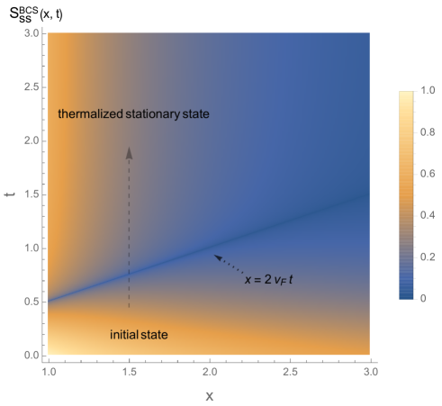
Figure 1: Space-time intensity plot of spin-singlet correlation function $S^{\mbox{\tiny BCS}}_{ss}(x,t)$ following a $U\to 0$ quench at $t=0$ from the BCS state. For short times below the light-cone boundary ($x=2v_{F}t$, appearing as a line of nodes feature), the correlation $S^{\mbox{\tiny BCS}}_{ss}(x,t)$ approaches the initial state one and thus varies similarly with $x$ for different $t$. For long times above the boundary, the time-dependence drops out and the system develops into thermalized stationary state, with correlations in agreement with the one of the post-quench free-fermion state at a finite temperature $T$ fixed by energy conservation.

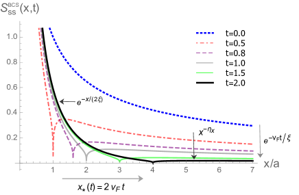
Figure 2: Spin-singlet pairing correlation function $S^{\mbox{\tiny BCS}}_{ss}(x,t)$ following a $U\to 0$ quench at $t=0$ from the BCS state for a series of times. The light-cone crossover, $x_{*}(t)=2v_{F}t$ separates exponential correlations $e^{-x/(2\xi)}$ at short scales, $x<x_{*}(t)$ from the power-law correlations $x^{-\eta_{x}}$ at long scales, $x>x_{*}(t)$. The latter power-law spatial correlations decay exponentially in time, as indicated by a vertical arrow on the right.

On the other hand, following the quench from an initial FFLO spin-gapless state to a noninteracting Fermi gas, we find that the dynamical spin-singlet pairing correlation function has the following asymptotics

$$\begin{split}S^{\mbox{\tiny FFLO}}_{ss}(x,t)&\sim\cos(k_{FFLO}x)\begin{cases}\left(\frac{a}{x}\right)^{\eta^{\prime}_{x}}\left(\frac{a}{2v_{F}t}\right)^{\eta^{\prime}_{t}},&x\gg 2v_{F}t,\\ \left(\frac{a}{x}\right)^{\eta^{\prime}_{x}+\eta^{\prime}_{t}},&x\ll 2v_{F}t,\end{cases}\end{split}$$ (2)

with the full expression given in Sec. IX.2, the intensity space-time profile illustrated in Fig. 3, and fixed time cuts plotted in Fig. 4. We observe that spatial oscillations at $k=k_{FFLO}$, characteristic of the FFLO initial state persist for all times, though at the light-cone time, $t_{*}(x)$ the spatial power-law amplitude of the initial state crosses over to a shorter-range power-law correlations. Despite that for longer times $t>t_{*}(x)$ the dephasing leads to a development of a stationary state, integrability together with the state’s gapless nature forbids full thermalization to exponential correlations of a free Fermi gas.

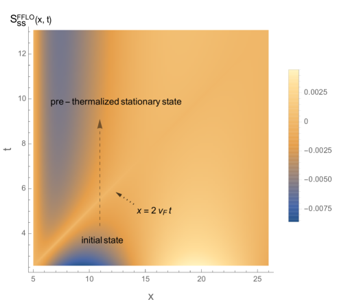
Figure 3: Space-time intensity plot of spin-singlet pairing correlation function $S^{\mbox{\tiny FFLO}}_{ss}(x,t)$ following a $U\to 0$ quench at $t=0$ from the FFLO state. In contrast to the BCS initial state, the correlations display spatial oscillations at the characteristic wavevector $k_{FFLO}$. A light-cone boundary $x=2v_{F}t$ distinguishing short- and long- time dynamics is visible.

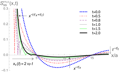
Figure 4: Spin-singlet pairing correlation function $S^{\mbox{\tiny FFLO}}_{ss}(x,t)$ following a $U\to 0$ quench at $t=0$ from the FFLO state for a series of times. A nonzero momentum spatial oscillations at $k=k_{FFLO}$ persist as the signature of the FFLO state, contrasting with Fig. 2 for the BCS state. The light-cone boundary, $x_{*}(t)=2v_{F}t$ separates a spatial power-law envelope $x^{-(\eta^{\prime}_{x}+\eta^{\prime}_{t})}$ at short scales, $x<x_{*}(t)$ from a shorter-range power-law $x^{-\eta^{\prime}_{x}}$ at long scales, $x>x_{*}(t)$. In the latter regime the overall amplitude decays as a power-law with time, indicated by a vertical arrow on the right.

We also computed the post-quench evolution of the density-density correlation function for quench from both spin-gapped BCS state and spin-gapless FFLO states. For the spin-gapped BCS state case, the density-density correlation is given by

$$\begin{split}&S^{\mbox{\tiny BCS}}_{nn}(x,t)\sim\\ &\begin{cases}-\gamma_{x}\frac{a^{2}}{x^{2}}+\left(\frac{a}{x}\right)^{\gamma_{x}}\left(\frac{2v_{F}t}{a}\right)^{\gamma_{t}}e^{-\frac{v_{F}t}{\xi}}\cos(2k_{F}x),&x\gg 2v_{F}t,\\ -\frac{\gamma_{t}}{2}\frac{a^{2}}{(x-2v_{F}t)^{2}},&x\approx 2v_{F}t,\\ -(\gamma_{x}-\gamma_{t})\frac{a^{2}}{x^{2}}+\left(\frac{a}{x}\right)^{\gamma_{x}-\gamma_{t}}e^{-\frac{x}{2\xi}}\cos(2k_{F}x),&x\ll 2v_{\sigma}t,\end{cases}\end{split}$$ (3)

and illustrated in Fig. 5. Here the space- and time- power-law exponents, $\gamma_{x,t}$ satisfy $0<\gamma_{t}<1<\gamma_{x}<2$. A striking feature of $S^{\mbox{\tiny BCS}}_{nn}(x,t)$ is the divergent peak associated with the light-cone boundary $x=2v_{F}t$. It delineates the short-time ($t<t_{*}(x)$) correlation of the initial state (that decay in time) and the long time ($t>t_{*}(x)$) regime where the stationary state emerges. In contrast to long-time pairing correlations, here the exponentially suppressed spin-gapped correlations are dominated by the gapless charge $1/x^{2}$ correlations. Similar results for the quench from the FFLO state are presented in Sec. IX.2.

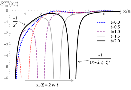
Figure 5: Density-density correlation function $S^{\mbox{\tiny BCS}}_{nn}(x,t)$ following a $U\to 0$ quench at $t=0$ from the BCS state for a series of times. The dominant features is the moving power-law peak $-1/(x-2v_{F}t)^{2}$ at the light-cone boundary.

Another interesting quantity is the magnetization and its correlations. In contrast to the mean-field oscillatory magnetization profile (qualitatively valid in higher dimensions), enhanced quantum fluctuations of the 1D geometry completely wash out this feature. However, they are manifested in the magnetization-magnetization correlation function which we illustrate in Sec. IX.

We next turn to the analysis of the 1D spin-imbalanced attractive Fermi-Hubbard model that leads to the above and a number of other results.

II Model and its bosonization

One-dimensional spin-imbalanced Fermi gas can be well-described by the Fermi-Hubbard model

$$\begin{split}\hat{H}=-t\sum_{\langle ij\rangle,\sigma}\hat{c}^{\dagger}_{i,\sigma}\hat{c}_{j,\sigma}-U\sum_{j}\hat{n}_{j\uparrow}\hat{n}_{j\downarrow}+h\sum_{j}(\hat{n}_{j\uparrow}-\hat{n}_{j\downarrow}),\end{split}$$ (4)

where $t$ is the nearest-neighbor hopping matrix element, $U$ the on-site attractive interaction and $h=(\mu_{\downarrow}-\mu_{\uparrow})/2$ the pseudo-Zeeman field. Throughout the paper, we work in the theoretically more convenient grand-canonical ensemble with the pseudospin- (species) imbalance $m=n_{j\uparrow}-n_{j\downarrow}$ tuned by h. For experiments conducted with fixed spin-imbalance, our theory can be easily applied by mapping h to m through the m(h) relation that we derived in Sec. V. Despite the accessibility of numerical approaches such as DMRG and exact diagonalization, in one dimension we can utilize the powerful analytical machinery of bosonization Coleman ; Giamarchi ; Tsvelik to obtain asymptotically exact behavior and to gain more physical insight.

Bosonization allows a representation of fermionic operators in terms of chiral bosonic phase fields, the phonon ${\hat{\phi}}$ and superfluid phase ${{\hat{\theta}}}$,

$$\begin{split}\hat{\psi}_{\sigma}(x_{j})=\frac{1}{\sqrt{2\pi a}}\hat{c}_{j,\sigma}=\hat{\psi}_{R\sigma}(x_{j})+\hat{\psi}_{L\sigma}(x_{j}),\end{split}$$ (5)

where $x_{j}=aj$ and

$$\begin{split}\hat{\psi}_{r,\sigma}(x)&=\hat{U}_{r,\sigma}\lim_{a\to 0}\frac{1}{\sqrt{2\pi a}}\\ &\quad\times e^{irk_{F}x}e^{-\frac{i}{\sqrt{2}}[r{\hat{\phi}}_{\rho}(x)-{{\hat{\theta}}}_{\rho}(x)+\sigma(r{\hat{\phi}}_{\sigma}(x)-{\hat{\theta}}_{\sigma}(x))]},\end{split}$$ (6)

with $r=\pm 1$ for right (R) and left (L) movers, and $\sigma=\pm 1$ for spin-up and spin-down, respectively. Here $a$ is an ultra-violet (UV) cutoff set by the lattice constant and $U_{r,\sigma}$ the standard Klein factor that ensures anti-commutation of fermionic operators. The bosonic phases satisfy the following commutation relations

$$\begin{split}[{\hat{\phi}}_{\rho}(x),\partial_{x^{\prime}}{\hat{\theta}}_{\rho}(x^{\prime})]&=i\pi\delta(x-x^{\prime}),\\ [{\hat{\theta}}_{\rho}(x),\partial_{x^{\prime}}{\hat{\phi}}_{\rho}(x^{\prime})]&=i\pi\delta(x-x^{\prime}),\\ [{\hat{\phi}}_{\sigma}(x),\partial_{x^{\prime}}{\hat{\theta}}_{\sigma}(x^{\prime})]&=i\pi\delta(x-x^{\prime}),\\ [{\hat{\theta}}_{\sigma}(x),\partial_{x^{\prime}}{\hat{\phi}}_{\sigma}(x^{\prime})]&=i\pi\delta(x-x^{\prime}).\end{split}$$ (7)

The charge $(\rho)$ and spin ($\sigma$) phase fields are given by

$$\begin{split}{\hat{\phi}}_{\rho}&=\frac{{\hat{\phi}}_{\uparrow}+{\hat{\phi}}_{\downarrow}}{\sqrt{2}},\;\;\;{\hat{\theta}}_{\rho}=\frac{{\hat{\theta}}_{\uparrow}+{\hat{\theta}}_{\downarrow}}{\sqrt{2}},\\ {\hat{\phi}}_{\sigma}&=\frac{{\hat{\phi}}_{\uparrow}-{\hat{\phi}}_{\downarrow}}{\sqrt{2}},\;\;\;{\hat{\theta}}_{\sigma}=\frac{{\hat{\theta}}_{\uparrow}-{\hat{\theta}}_{\downarrow}}{\sqrt{2}},\end{split}$$ (8)

respectively. Using above relations and taking the continuum limit, the Hubbard Hamiltonian can be re-expressed in terms of the bosonic fields,

$$\begin{split}\hat{H}&=\hat{H}_{\rho}+\hat{H}_{\sigma},\end{split}$$ (9)

to lowest order separating into the charge sector,

$$\begin{split}\hat{H}_{\rho}&=\frac{v_{\rho}}{2\pi}\int dx\left[\frac{1}{K_{\rho}}(\partial_{x}{\hat{\phi}}_{\rho})^{2}+K_{\rho}(\partial_{x}{\hat{\theta}}_{\rho})^{2}\right],\end{split}$$ (10)

and the spin sector,

$$\begin{split}\hat{H}_{\sigma}&=\frac{v_{\sigma}}{2\pi}\int dx\left[\frac{1}{K_{\sigma}}(\partial_{x}{\hat{\phi}}_{\sigma})^{2}+K_{\sigma}(\partial_{x}{\hat{\theta}}_{\sigma})^{2}\right]\\ &\quad-\frac{U}{2\pi^{2}a}\int dx\cos(\sqrt{8}{\hat{\phi}}_{\sigma})-\frac{\sqrt{2}h}{\pi}\int dx\partial_{x}{\hat{\phi}}_{\sigma}.\end{split}$$ (11)

Above we have neglected the spin-imbalance-induced spin-charge coupling that is weak for $m/k_{F}\sim(k_{F\uparrow}-k_{F\downarrow})/k_{F}\ll 1$ VincentLiuPRA ; Rizzi . The parameters $K_{\rho,\sigma}$ and $v_{\rho,\sigma}$ are, respectively, the Luttinger parameters and the velocities for the charge and spin part, respectively, and are perturbatively [in $Ua/(\pi v_{F})$] related to the original Hubbard model parameters through

$$\begin{split}v_{F}&=2ta\sin(k_{F}a),\\ v_{\rho}&=v_{F}\sqrt{1-\frac{Ua}{\pi v_{F}}},\\ v_{\sigma}&=v_{F}\sqrt{1+\frac{Ua}{\pi v_{F}})},\\ \frac{1}{K_{\rho}}&=\sqrt{1-\frac{Ua}{\pi v_{F}}},\\ \frac{1}{K_{\sigma}}&=\sqrt{1+\frac{Ua}{\pi v_{F}}}.\end{split}$$ (12)

For the strong interaction above relations break down, but are well known to satisfy $K_{\rho}\to 2$ and $K_{\sigma}\to 1/2$ in the $U\to\infty$ limit Giamarchi .

To probe the system, we focus on a variety of correlation functions of the spin-singlet and triplet pairing operators:

$$\hat{O}_{ss}(x) =\hat{\psi}^{\dagger}_{R\uparrow}\hat{\psi}^{\dagger}_{L\downarrow}+\hat{\psi}^{\dagger}_{L\uparrow}\hat{\psi}^{\dagger}_{R\downarrow}=\frac{1}{\pi a}e^{-i\sqrt{2}{\hat{\theta}}_{\rho}}\cos(\sqrt{2}{\hat{\phi}}_{\sigma}),$$ (13a)

$$\hat{O}_{st}(x) =\hat{\psi}^{\dagger}_{R\uparrow}\hat{\psi}^{\dagger}_{L\uparrow}+\hat{\psi}^{\dagger}_{L\downarrow}\hat{\psi}^{\dagger}_{R\downarrow}=\frac{1}{\pi a}e^{-i\sqrt{2}{\hat{\theta}}_{\rho}}\cos(\sqrt{2}{\hat{\theta}}_{\sigma}),$$ (13b)

as well as of the number and magnetization density operators,

$$\hat{n}(x) =\hat{\psi}^{\dagger}_{\uparrow}\hat{\psi}_{\uparrow}+\hat{\psi}^{\dagger}_{\downarrow}\hat{\psi}_{\downarrow}=-\frac{\sqrt{2}}{\pi}\partial_{x}{\hat{\phi}}_{\rho}(x)+\hat{O}_{CDW}+h.c.,$$ (14a)

$$\hat{m}(x) =\hat{\psi}^{\dagger}_{\uparrow}\hat{\psi}_{\uparrow}-\hat{\psi}^{\dagger}_{\downarrow}\hat{\psi}_{\downarrow}=-\frac{\sqrt{2}}{\pi}\partial_{x}{\hat{\phi}}_{\sigma}(x)+\hat{O}^{z}_{SDW}+h.c.,$$ (14b)

where, respectively, the charge- and spin-density wave operators,

$$\hat{O}_{CDW}(x) =\hat{\psi}^{\dagger}_{R\uparrow}\hat{\psi}_{L\uparrow}+\hat{\psi}^{\dagger}_{R\downarrow}\hat{\psi}_{L\downarrow}=\frac{e^{-2ik_{F}x}}{\pi a}e^{i\sqrt{2}{\hat{\phi}}_{\rho}}\cos(\sqrt{2}{\hat{\phi}}_{\sigma}),$$ (15a)

$$\hat{O}^{z}_{SDW}(x) =\hat{\psi}^{\dagger}_{R\uparrow}\hat{\psi}_{L\uparrow}-\hat{\psi}^{\dagger}_{R\downarrow}\hat{\psi}_{L\downarrow}=\frac{e^{-2ik_{F}x}}{\pi a}e^{i\sqrt{2}{\hat{\phi}}_{\rho}}i\sin(\sqrt{2}{\hat{\phi}}_{\sigma}).$$ (15b)

are defined as the oscillatory part of the density component.

Thus in the bosonized form, the spin-singlet pairing correlation is given by

$$\begin{split}S_{ss}(x)&\equiv(\pi a)^{2}\langle\hat{O}_{ss}(x)\hat{O}^{\dagger}_{ss}(0)\rangle,\\ &=\langle e^{-i\sqrt{2}[{\hat{\theta}}_{\rho}(x)-{\hat{\theta}}_{\rho}(0)]}\rangle\langle\cos(\sqrt{2}{\hat{\phi}}_{\sigma}(x))\cos(\sqrt{2}{\hat{\phi}}_{\sigma}(0))\rangle,\end{split}$$ (16)

and its triplet counterpart is given by

$$\begin{split}S_{st}(x)&\equiv(\pi a)^{2}\langle\hat{O}_{ts}(x)\hat{O}^{\dagger}_{ts}(x)\rangle,\\ &=\langle e^{-i\sqrt{2}[{\hat{\theta}}_{\rho}(x)-{\hat{\theta}}_{\rho}(0)]}\rangle\langle\cos(\sqrt{2}{\hat{\theta}}_{\sigma}(x))\cos(\sqrt{2}{\hat{\theta}}_{\sigma}(0))\rangle.\end{split}$$ (17)

Similarly, the density-density and magnetization-magnetization correlation functions are given by

$$S_{nn}(x) \equiv(\pi a)^{2}\langle\hat{n}(x)\hat{n}(0)\rangle$$

$$=2a^{2}\langle\partial_{x}{\hat{\phi}}_{\rho}(x)\partial_{x^{\prime}}{\hat{\phi}}_{\rho}(0)\rangle+2\cos(2k_{F}x)\langle e^{i\sqrt{2}[{\hat{\phi}}_{\rho}(x)-{\hat{\phi}}_{\rho}(0)}\rangle$$

$$\quad\times\langle\cos(\sqrt{2}({\hat{\phi}}_{\sigma}(x))\cos(\sqrt{2}{\hat{\phi}}_{\sigma}(0))\rangle,$$ (18a)

$$S_{mm}(x) \equiv(\pi a)^{2}\langle\hat{m}(x)\hat{m}(0)\rangle$$

$$=2a^{2}\langle\partial_{x}{\hat{\phi}}_{\sigma}(x)\partial_{x^{\prime}}{\hat{\phi}}_{\sigma}(0)\rangle-2\cos(2k_{F}x)\langle e^{i\sqrt{2}[{\hat{\phi}}_{\rho}(x)-{\hat{\phi}}_{\rho}(0)}\rangle$$

$$\quad\times\langle\sin(\sqrt{2}{\hat{\phi}}_{\sigma}(x))\sin(\sqrt{2}{\hat{\phi}}_{\sigma}(0))\rangle.$$ (18b)

Having recalled the basic formalism, in the next few sections we will utilize it to compute the ground-state properties of the spin-imbalanced attractive Fermi-Hubbard model, and will then utilize these to calculate the post-quench dynamics of the corresponding correlators.

III charge sector

As mentioned in last section, one prominent feature of 1D system is the spin-charge separation. Utilizing this property, we briefly review the equilibrium charge sector results in this section to further define our notations and set stage for dynamical analysis of future sections.

The charge sector is described by the quadratic Hamiltonian (10) that can therefore be easily diagonalized. Expressing ${\hat{\phi}}_{\rho}$ and ${\hat{\theta}}_{\rho}$ in terms of bosonic creation and annihilation operators $\hat{b}^{\dagger}_{p}$ and $\hat{b}_{p}$

$${\hat{\phi}}(x)=-\frac{i\pi}{L}\sum_{p\neq 0}\left(\frac{L|p|}{2\pi}\right)^{1/2}\frac{1}{p}e^{-a|p|/2-ipx}(\hat{b}^{\dagger}_{p}+\hat{b}_{-p}),$$ (19a)

$${\hat{\theta}}(x)=\frac{i\pi}{L}\sum_{p\neq 0}\left(\frac{L|p|}{2\pi}\right)^{1/2}\frac{1}{|p|}e^{-a|p|/2-ipx}(\hat{b}^{\dagger}_{p}-\hat{b}_{-p}),$$ (19b)

the resulting Hamiltonian

$$\begin{split}\hat{H}_{\rho}&=\frac{1}{4}\sum_{p\neq 0}v_{\rho}|p|\Big{[}(1/K_{\rho}+K_{\rho})(\hat{b}^{\dagger}_{p}\hat{b}_{p}+\hat{b}^{\dagger}_{-p}\hat{b}_{-p})\\ &\quad+(1/K_{\rho}-K_{\rho})(\hat{b}^{\dagger}_{p}\hat{b}^{\dagger}_{-p}+\hat{b}_{p}\hat{b}_{-p})\Big{]}\end{split}$$ (20)

is straightforwardly diagonalized by a bosonic Bogoliubov transformation

$$\begin{split}\begin{pmatrix}\hat{b}_{p}\\ \hat{b}^{\dagger}_{-p}\end{pmatrix}=\begin{pmatrix}\cosh\beta&-\sinh\beta\\ -\sinh\beta&\cosh\beta\end{pmatrix}\begin{pmatrix}\hat{\chi}_{p}\\ \hat{\chi}^{\dagger}_{-p}\end{pmatrix},\end{split}$$ (21)

giving

$$\hat{H}_{0}=\sum_{p\neq 0}v_{\rho}|p|\hat{\chi}^{\dagger}_{p}\hat{\chi}_{p}$$ (22)

with $e^{-2\beta}=K_{\rho}$.

Using the zero-temperature ground-state distribution $\langle\hat{\chi}_{p}\hat{\chi}^{\dagger}_{p^{\prime}}\rangle=\delta_{p,{p^{\prime}}}$, one then obtains

$$\langle e^{\sqrt{2}i({\hat{\phi}}_{\rho}(x)-{\hat{\phi}}_{\rho}(0))}\rangle =e^{-\langle[{\hat{\phi}}_{\rho}(x)-{\hat{\phi}}_{\rho}(0)]^{2}\rangle},$$ (23a)

$$\sim e^{K_{\rho}\int^{\infty}_{0}{dp}/{p}e^{-ap}[1-\cos(px)]},$$

$$\sim\left(\frac{a}{x}\right)^{K_{\rho}},$$ (23b)

and

$$\langle e^{\sqrt{2}i({\hat{\theta}}_{\rho}(x)-{\hat{\theta}}_{\rho}(0))}\rangle =e^{-\langle[{\hat{\theta}}_{\rho}(x)-{\hat{\theta}}_{\rho}(0)]^{2}\rangle},$$ (24a)

$$\sim e^{{1}/{K_{\rho}}\int^{\infty}_{0}{dp}/{p}e^{-ap}[1-\cos(px)]},$$

$$\sim\left(\frac{a}{x}\right)^{1/K_{\rho}},$$ (24b)

where in Eqs. (23a) and (24a), we have used Wick’s theorem,

$$\langle e^{i\hat{A}}\rangle=e^{-\frac{1}{2}\langle\hat{A}^{2}\rangle},$$ (25)

valid for any free (i.e., Guassian) field operator $\hat{A}$.

The other component that enters the density-density correlation function can now also be straightforwardly calculated to be

$$\begin{split}\partial_{x}\partial_{x^{\prime}}\langle{\hat{\phi}}_{\rho}(x){\hat{\phi}}_{\rho}(x^{\prime})\rangle&=-\frac{1}{2}\partial_{x}\partial_{x^{\prime}}\langle({\hat{\phi}}_{\rho}(x)-{\hat{\phi}}_{\rho}(x^{\prime}))^{2}\rangle,\\ &\sim-\frac{K_{\rho}}{2(x-x^{\prime})^{2}}.\end{split}$$ (26)

We next turn to the analysis of the spin sector of the model.

IV spin sector: Luther-Emery exact analysis

The analysis of the spin sector Hamiltonian (11) is a bit more challenging due to the cosine nonlinearity (associated with the attractive pairing interaction), the so-called sine-Gordon model. While in principle the model is integrable, its correlation functions are still difficult to compute and generically approximate methods (perturbation theory, semiclassics, and renormalization group) need to be employed. However, for a spin Luttinger parameter $K_{\sigma}=1/2$ (the LE point) the model is exactly solvable through a mapping (re-fermionization) onto free spinless fermions (the solitons), with the cosine nonlinearity reducing to a mass that backscatters between the left and right movers LutherEmery ; JaparidzeNersesyan ; CazalillaJOP . The commensurate-incommensurate (PT) BCS-FFLO transition PokrovskyTalapov , driven by the Zeeman field $h$ then maps onto a simple conduction band filling with chemical potential $h$ and gap set by the Hubbard $U$ (see Fig. 6). The LE approach thus provides a clear physical picture of the spin-gapped BCS and gapless FFLO paired states and serves as a benchmark for other approximate solutions needed away from the $K_{\sigma}=1/2$ point.

The essential component of LE is that the nonlinearity $\cos(2\sqrt{2}{\hat{\phi}}_{\sigma})$ in the spin sector, Eq. (11) (generated from the interaction of the original fermions) for $K_{\sigma}=1/2$ can be “re-fermionized” into a quadratic backscattering mass term,

$$\begin{split}\hat{c}^{\dagger}_{R}(x)\hat{c}_{L}(x)=\frac{1}{2\pi a}e^{i2{\hat{\phi}}(x)},\end{split}$$ (27)

between new left and right moving, spinless Dirac fermions ($r=R,L$),

$$\begin{split}\hat{c}_{r}(x)&=U_{r}\lim_{a\to 0}\frac{1}{\sqrt{2\pi a}}e^{-i(r{\hat{\phi}}(x)-{\hat{\theta}}(x))}.\end{split}$$ (28)

This can be seen by rescaling $\sqrt{2}{\hat{\phi}}_{\sigma}\equiv{\hat{\phi}}$ and ${\hat{\theta}}_{\sigma}/\sqrt{2}\equiv{\hat{\theta}}$ (to retain the canonical commutation relation) into new bosonic fields, controlled by an effective Luttinger parameter $K\equiv 2K_{\sigma}$.

For $K=1$ ($K_{\sigma}=1/2$), the bosonic Hamiltonian can be re-fermionized into a noninteracting massive Thirring model Coleman ,

$$\hat{H} =\sum_{p}(v_{\sigma}p+h)\hat{c}^{\dagger}_{Rp}\hat{c}_{Rp}+(-v_{\sigma}p+h)\hat{c}^{\dagger}_{Lp}\hat{c}_{Lp}$$

$$\quad-\frac{U}{\pi}\sum_{p}\hat{c}^{\dagger}_{Rp}\hat{c}_{Lp}+h.c.,$$ (29a)

$$\equiv\sum_{p}\hat{\psi}^{\dagger}(p)H(p)\hat{\hat{\psi}}(p),$$ (29b)

where

$$\begin{split}\hat{\psi}(p)=\begin{bmatrix}\hat{c}_{R}(p)\\ \hat{c}_{L}(p)\\ \end{bmatrix},\;\;\;\;H(p)=\begin{bmatrix}v_{\sigma}p+h&-U/\pi\\ -U/\pi&-v_{\sigma}p+h\\ \end{bmatrix},\end{split}$$ (30)

The latter is diagonalized by a Bogoliubov transformation

$$\begin{split}{\hat{\psi}}(p)=\begin{bmatrix}\hat{c}_{u}(p)\\ \hat{c}_{l}(p)\\ \end{bmatrix}=\begin{bmatrix}\cos\beta_{p}&\sin\beta_{p}\\ -\sin\beta_{p}&\cos\beta_{p}\\ \end{bmatrix}\begin{bmatrix}\hat{c}_{R}(p)\\ \hat{c}_{L}(p)\\ \end{bmatrix},\end{split}$$ (31)

where $\tan 2\beta_{p}=-U/(\pi v_{\sigma}p)$ and lower-index $u,l$ denotes the upper and lower bands, respectively. This gives

$$\begin{split}\hat{H}=\sum_{p}\omega(p)[\hat{c}^{\dagger}_{u}(p)\hat{c}_{u}(p)-\hat{c}^{\dagger}_{l}(p)\hat{c}_{l}(p)],\end{split}$$ (32)

with a spin-gapped excitation spectrum

$$\omega(p)=\pm\sqrt{v^{2}_{\sigma}p^{2}+U^{2}/\pi^{2}},\ \ \ \Delta\equiv U/\pi.$$ (33)

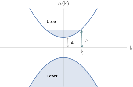
Figure 6: Band structure for spinless fermions for a spin gap $\Delta$ with the chemical potential $h$. For $h>h_{c}=\Delta$, the lower-band is completely filled, and the upper band is partially filled upto the Fermi momentum $\tilde{k}_{F}(h)$ (determined by the effective chemical potential $h$), that gives the magnetization (species imbalance) density.

This band structure is illustrated in Fig. 6.

IV.1 BCS state

Thus, as illustrated in Fig. 6, for the effective chemical potential $h$ less than the critical spin-gap value $h_{c}=\Delta$, i.e., for $h<\Delta\equiv U/\pi$, only the lower band is filled,

$$\langle\hat{c}^{\dagger}_{l}(p)\hat{c}_{l}(p)\rangle =1,$$ (34a)

$$\langle\hat{c}^{\dagger}_{u}(p)\hat{c}_{u}(p)\rangle =0,$$ (34b)

the system is fully gapped and this ground state corresponds to the spin-gapped BCS (soliton vacuum) phase, with a vanishing magnetization (number density of fermions in the upper band). The corresponding occupation of the spinless fermions $\hat{c}_{R,L}$ is then given by the Bogoliubov transformation Eq. (31)

$$\langle\hat{c}^{\dagger}_{R}(p)\hat{c}_{R}(p)\rangle =\sin^{2}\beta_{p},$$ (35a)

$$\langle\hat{c}^{\dagger}_{L}(p)\hat{c}_{L}(p)\rangle =\cos^{2}\beta_{p},$$ (35b)

$$\langle\hat{c}^{\dagger}_{R}(p)\hat{c}_{L}(p)\rangle =-\frac{1}{2}\sin 2\beta_{p}.$$ (35c)

Thus, the correlators of the nontrivial bosonic sine-Gordon theory, that can be simply expressed in terms of these noninteracting fermions, can be straightforwardly calculated. For example (leaving details to Appendix A) LutherEmery ; JaparidzeNersesyan

$$\begin{split}\langle e^{i\sqrt{2}[{\hat{\theta}}_{\sigma}(x)-{\hat{\theta}}_{\sigma}(0)]}\rangle&\sim\frac{a^{2}}{x^{2}}e^{-2x/\xi},\end{split}$$ (36)

where

$$\xi=\pi v_{\sigma}/U$$ (37)

is the correlation length. Also, the long-wavelength part of the magnetization correlator is given by

$$\begin{split}\langle\partial_{x}{\hat{\phi}}_{\sigma}(x)\partial_{x^{\prime}}{\hat{\phi}}_{\sigma}(0)\rangle&\sim-\frac{1}{2\pi\xi x}e^{-2x/\xi}.\end{split}$$ (38)

IV.2 FFLO state

On the other hand, for the chemical potential $h$ larger than the spin gap $\Delta$, the upper band fills partially up to a Fermi momentum, $\tilde{k}_{F}=\sqrt{h^{2}-U^{2}/\pi^{2}}/v_{\sigma}\sim\sqrt{h-h_{c}}$,

$$\begin{split}\langle\hat{c}^{\dagger}_{l}(p)\hat{c}_{l}(p)\rangle&=1,\\ \langle\hat{c}^{\dagger}_{u}(p)\hat{c}_{u}(p)\rangle&=\Theta(\tilde{k}_{F}-|k|),\\ \end{split}$$ (39)

corresponding to a proliferation of solitons into the spin-gapless FFLO ground state, characterized by a nonzero magnetization,

$$\begin{split}\bar{m}&=\frac{\sqrt{2}}{\pi}\tilde{k}_{F}=\frac{\sqrt{2}}{\pi v_{\sigma}}\sqrt{h^{2}-U^{2}/\pi^{2}}\sim\sqrt{h-h_{c}}.\end{split}$$ (40)

The ${\hat{\theta}}_{\sigma}$ correlation functions are then given by

$$\begin{split}\langle e^{i\sqrt{2}[{\hat{\theta}}_{\sigma}(x)-{\hat{\theta}}_{\sigma}(0)]}\rangle&\sim(\tilde{k}_{F}\xi)^{2}\frac{a^{2}}{x^{2}},\end{split}$$ (41)

and

$$\begin{split}\langle\partial_{x}{\hat{\phi}}_{\sigma}(x)\partial_{x^{\prime}}{\hat{\phi}}_{\sigma}(0)\rangle&\sim-\frac{\sin^{2}(\tilde{k}_{F}x)}{\pi^{2}x^{2}},\end{split}$$ (42)

which, as expected resembles the density-density correlator of free spinless fermions, but differs drastically from the exponentially decaying spin-gapped BCS result.

V Spin sector: semiclassical approach

Away from the Luther-Emery point, the interaction between LE fermions precludes an exact solution for arbitrary $K_{\sigma}\neq 1/2$, but the structure of the phase diagram and nature of the phases are expected to remain qualitatively the same. We instead proceed with a semiclassical approach by studying quantum fluctuations about the classical (time-independent) saddle-point solution ${\phi}_{\sigma}^{0}$ for the model (11), satisfying the sine-Gordon equation, with an intrinsic length scale $\lambda=\sqrt{\frac{\pi av_{\sigma}}{8K_{\sigma}U}}$.

V.1 BCS state

For $h<h_{c}$, the stable state is a soliton vacuum (spin-gapped BCS) ground state, characterized by ${\phi}_{\sigma}^{0}=0$ in the bulk. With free boundary conditions in a finite length $L$ system, for a finite $h$, the tilt (magnetization) $\partial_{x}\phi^{0}_{\sigma}(\pm L/2)=\sqrt{2}K_{\sigma}h/v_{\sigma}$ “penetrates” into the sample within an $h$-dependent length $\lambda(h)$ (a fraction of a soliton), as schematically illustrated in Fig. 7. At the classical level (ignoring quantum fluctuations) $h_{c}^{(cl)}$ is determined by the condition that the tilt at the boundary is $~{}1/\lambda$, i.e., $h_{c}^{(cl)}\sim v_{\sigma}/\lambda\sim\sqrt{U}$, a point beyond which a soliton of width $\lambda$ can enter the bulk.

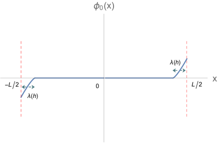
Figure 7: Schematic illustration of the classical spin-gapped solution $\phi^{0}_{\sigma}(x)$ for a finite system of size $L$, (nearly) vanishing in the bulk, but with a finite tilt (magnetization) penetrating a length $\lambda(h)<\lambda$ at the edges.

We observe that the critical field $h_{c}^{(cl)}$ and characteristic length $\lambda$ differ qualitatively from their LE (exact) counterparts of $h_{c}=U/\pi$ and correlation length $\xi=v_{\sigma}/h_{c}$, (37). This is a consequence of quantum fluctuations.

Within the spin-gapped BCS state ${\hat{\phi}}_{\sigma}$ is localized in a minimum of the cosine potential (at its classical solution ${\phi}_{\sigma}^{0}=0$), and can be safely expanded in small quadratic fluctuations governed by CazalillaJOP

$$\begin{split}\delta\hat{H}_{\sigma}&=\frac{v_{\sigma}}{2\pi}\int dx[\frac{1}{K_{\sigma}}(\partial_{x}{\hat{\phi}}_{\sigma})^{2}+K_{\sigma}(\partial_{x}{\hat{\theta}}_{\sigma})^{2}]\\ &\quad+\frac{2U}{\pi^{2}a}\int dx({\hat{\phi}}_{\sigma})^{2}-\frac{\sqrt{2}h}{\pi}\int dx\partial_{x}{\hat{\phi}}_{\sigma}.\end{split}$$ (43)

The corresponding Hamiltonian in terms of bosonic operators $\hat{b}_{p},\hat{b}^{\dagger}_{p}$ can be straightforwardly diagonalized via

$$\begin{split}\begin{bmatrix}\hat{b}_{p}\\ \hat{b}^{\dagger}_{-p}\\ \end{bmatrix}=\begin{bmatrix}u_{p}&-v_{p}\\ -v_{p}&u_{p}\\ \end{bmatrix}\begin{bmatrix}\hat{\alpha}_{p}\\ \hat{\alpha}^{\dagger}_{-p}\\ \end{bmatrix},\end{split}$$ (44)

with $\delta\hat{H}_{\sigma}=\sum_{p}\omega(p)\hat{\alpha}^{\dagger}_{p}\hat{\alpha}_{p}$, where

$$\begin{split}u^{2}_{p}&=\frac{1}{2}\left(\frac{|p|+{1}/(2\lambda^{2}p)}{\sqrt{p^{2}+1/\lambda^{2}}}+1\right),\\ v^{2}_{p}&=\frac{1}{2}\left(\frac{|p|+{1}/(2\lambda^{2}p)}{\sqrt{p^{2}+1/\lambda^{2}}}-1\right),\end{split}$$ (45)

and the spectrum is given by

$$\begin{split}\omega_{p}=\pm v_{\sigma}\sqrt{p^{2}+1/\lambda^{2}},\end{split}$$ (46)

with the gap $\Delta_{0}=v_{\sigma}/\lambda$.

At $T=0$, in the ground state,

$$\langle\hat{b}^{\dagger}_{p}\hat{b}_{p}\rangle =\langle\hat{b}^{\dagger}_{-p}\hat{b}_{-p}\rangle=v^{2}_{p},$$ (47a)

$$\langle\hat{b}^{\dagger}_{p}\hat{b}^{\dagger}_{-p}\rangle =\langle\hat{b}_{p}\hat{b}_{-p}\rangle=-u_{p}v_{p},$$ (47b)

which (relegating the details to Appendix B) gives

$$\langle e^{i\sqrt{2}[{\hat{\phi}}_{\sigma}(x)-{\hat{\phi}}_{\sigma}(0)]}\rangle \sim\operatorname{const},$$ (48a)

$$\langle e^{i\sqrt{2}[{\hat{\theta}}_{\sigma}(x)-{\hat{\theta}}_{\sigma}(0)]}\rangle \sim e^{-x/\xi_{0}},$$ (48b)

with $\xi_{0}=2\lambda K_{\sigma}/\pi$, and demonstrating the stability of the spin-gapped state to quantum fluctuations.

The leading exponential decay in the correlator in (48) agrees qualitatively with one predicted by the exact LE analysis (36) $K_{\sigma}=1/2$, though at this level of calculation misses the subdominant power-law prefactor.

However, one obvious discrepancy is that the semiclassically computed correlation length $\xi_{0}=\sqrt{av_{\sigma}K/2\pi U}\sim\sqrt{1/U}$ in Eq. (48) differs from $\xi=\pi v_{\sigma}/U\sim 1/U$ in Eq. (36), obtained using the exact LE approach. This can be understood by noting that for small $U$ (such that $\xi_{0}\gg a$), for high momentum modes $\xi_{0}^{2}k^{2}>(ka)^{2K_{\sigma}}$ the cosine pinning potential is weaker than the elastic (density interaction) energy and thus contribute divergently and nonperturbatively to renormalize the correlation length. Indeed a standard RG analysis gives $\xi_{0}\rightarrow a(\xi_{0}/a)^{2/(2-2K_{\sigma})}\sim 1/U^{1/(2-2K_{\sigma})}$, which for $K_{\sigma}=1/2$ scales as $1/U$, reassuringly consistent with LE.

V.2 FFLO state

For $h>h_{c}$, the spin-gapped ground state ${\phi}_{\sigma}^{0}=0$ is unstable to soliton proliferation in the bulk, leading to the FFLO. At the semiclassical level this takes place when the $h$-imposed tilt at the boundary reaches $1/\lambda$, allowing solitons to penetrate into the bulk; more generally the transition is associated with the soliton (LE fermions in the upper band) gap closing.

The corresponding semiclassical solution to the sine-Gordon equation is a soliton lattice, extensively studied in the literature Hanna , is illustrated in Fig. 9 with spacing $d=\bar{m}^{-1}$ and width $\lambda$,

$$\begin{split}{\phi}_{\sigma}^{0}(x)=\frac{1}{\sqrt{2}}\operatorname{am}(x/(\sqrt{2}\lambda k),k).\end{split}$$ (49)

Above $am(x,k)$ is the Jacobi amplitude function, parameterized by the $h$-dependent parameter $k$ (ranging from $0$ to $1$, not to be confused with the momentum $k$) that controls the soliton density. Minimizing the energy over $k$ gives the equation that determines $k$ (see also Fig. 8):

$$\begin{split}\frac{E(k)}{k}=\frac{h}{h_{c}},\end{split}$$ (50)

where $h_{c}=2v_{\sigma}/(\pi\lambda K_{\sigma})$ and $E(k)$ the Jacobi elliptic function (not to be confused with the spectrum $E$).

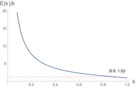
Figure 8: Plot of $E(k)/k$ [Eq. (50)] as a function of the index $k$, with the soliton solution characterized by $0<k<1$ stable for $h>h_{c}$. For $h/h_{c}=1.3$, indicated by the red dashed line, the corresponding index is $k=0.9$.

At large $h\gg h_{c}$ the solution quickly approaches a sloped straight line, corresponding to a dense soliton lattice, with $\bar{m}\sim h/(h_{c}\lambda)$ deep in the incommensurate phase with ${\phi}_{\sigma}^{0}(x)=\bar{m}x$.

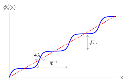
Figure 9: Schematic plot of the soliton lattice solution ${\phi}_{\sigma}^{0}$ for (49) as a function of $x$. $\bar{m}^{-1}$ and $\lambda$ are two length scales that characterize the average soliton lattice, the soliton spacing (density $\bar{m}$) and width, respectively. The straight line is a guide to an eye.

The magnetization in the FFLO state is set by the soliton density, which is illustrated in Fig. 10, and given by

$$\begin{split}\bar{m}_{cl}&=\frac{1}{2\sqrt{2}\lambda kK(k)}\\ &\sim\frac{1}{2\sqrt{2}\lambda}\begin{cases}-\frac{h}{h_{c}}1/\ln(\frac{h}{h_{c}}-1),&\mbox{for }h/h_{c}\to 1,\\ \frac{4}{\pi^{2}}\frac{h}{h_{c}},&\mbox{for }h/h_{c}\to\infty,\end{cases}\end{split}$$ (51)

with $k(h)$ tuned by the Zeeman field $h$ through Eq. (50).

This fast logarithmic growth is associated with (in the absence of fluctuations) the exponential weakness of soliton interactions near $h_{c}$ where solitons are dilute. Because of this, the soliton density rises to nearly densely packed value of order $1/\lambda$, at which point $\bar{m}(h)$ is a linear function of $h$. Quantum (and thermal) fluctuations qualitatively modify these predictions as is clear from the exact LE analysis, $\bar{m}\sim\sqrt{h^{2}-h_{c}^{2}}$, and more generally from an array of fluctuating soliton world lines PokrovskyTalapov .

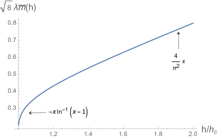
Figure 10: Plot of magnetization $\bar{m}_{cl}$ (within a classical approximation) as a function $h/h_{c}$ [see Eq. (51)]. Within the critical region, $\bar{m}\propto-x\ln^{-1}(x-1)$ and away from critical region it is well approximated by a linear function.

To include quantum fluctuations about this classical description of the FFLO state is quite nontrivial. To simplify the analysis, we limit our study outside of the critical region at $h_{c}$. As illustrated in Fig. 11, in this regime, even for a fairly modest $h/h_{c}=1.3$ solitons strongly overlap and the classical solution is given by

Figure 11: Classical soliton lattice solution ${\phi}_{\sigma}^{0}$ (49) as a function of $x/\lambda$ for $h/h_{c}=1.3$, as compared with the approximate dashed straight line solution (52).

$$\begin{split}{\phi}_{\sigma}^{0}(x)\approx\frac{1}{\sqrt{2}}\operatorname{am}(2K(k)\bar{m}x)&\approx\frac{h}{\pi h_{c}}\frac{x}{\lambda}\approx\frac{\pi\bar{m}}{\sqrt{2}}x.\end{split}$$ (52)

Quantum fluctuations are naturally included through the phonons $\tilde{\phi}(x)$ of the soliton lattice, which can thereby be related to the original bosonic fields,

$$\begin{split}{\hat{\phi}}_{\sigma}=\frac{1}{\sqrt{2}}(\pi\bar{m}x+\tilde{\phi}(x)),\end{split}$$ (53)

and correspondingly for the conjugate phase,

$$\begin{split}{\hat{\theta}}_{\sigma}=\sqrt{2}\tilde{\theta}(x),\end{split}$$ (54)

crucial for computation of physical observables. This is consistent with the LE construction, where at finite $h\gg h_{c}$ the upper band spinless fermions around $\pm\tilde{k}_{F}$ can be re-bosonized (see Fig. 12), with the Hamiltonian Shoucheng ,

$$\begin{split}\tilde{H}_{FFLO}&=\frac{\tilde{v}}{2\pi}\int dx\left[\frac{1}{\kappa}(\partial_{x}\tilde{\phi})^{2}+\kappa(\partial_{x}\tilde{\theta})^{2}\right],\end{split}$$ (55)

where $\tilde{v}$ and $\kappa$ are the new set of Luttinger parameters.

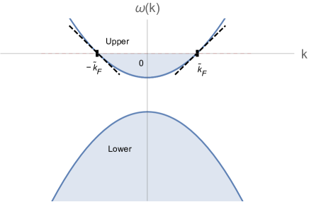
Figure 12: Re-bosonization near the new Fermi points $\pm\tilde{k}_{F}$, determined by spin-imbalance $h$ for the upper-band spinless fermions.

At the LE $K_{\sigma}=1/2$ point the fermions are noninteracting and so $\kappa=1$. Perturbative analysis around the LE point gives Schulz

$$\begin{split}\kappa=1+\frac{v_{\sigma}\bar{m}\pi a}{U}\left(2K_{\sigma}-\frac{1}{2K_{\sigma}}\right),\end{split}$$ (56)

Furthermore, near the transition at $h_{c}$ the LE fermion (soliton) density $\bar{m}$ vanishes and we expect $\kappa$ to also approach $1$.

Utilizing the relation (53,54), standard analysis of the original bosonic fields then gives ${\hat{\phi}}_{\sigma}$ and ${\hat{\theta}}_{\sigma}$ correlators

$$\langle e^{i\sqrt{2}({\hat{\phi}}_{\sigma}(x)-{\hat{\phi}}_{\sigma}(0))}\rangle \sim e^{i\pi\bar{m}x}\left|\frac{a}{x}\right|^{\kappa/2},$$ (57a)

$$\langle e^{i\sqrt{2}({\hat{\theta}}_{\sigma}(x)-{\hat{\theta}}_{\sigma}(0))}\rangle \sim{\left|\frac{a}{x}\right|^{2/\kappa}},$$ (57b)

$$\frac{{2}}{\pi^{2}}\langle\partial_{x}{\hat{\phi}}_{\sigma}(x)\partial_{x^{\prime}}{\hat{\phi}}_{\sigma}(0)\rangle \sim-\frac{\kappa}{2\pi^{2}x^{2}}.$$ (57c)

Comparing these with the non-interacting fermion correlators also allows us to infer that $\kappa\rightarrow 2$, as $U\rightarrow 0$.

VI 1D spin-imbalanced Fermi-Hubbard model: Equilibrium

We can now combine the above results for charge and spin sectors to obtain the ground-state correlators for the 1D spin-imbalanced attractive Fermi-Hubbard model (4).

VI.1 Spin-gapped (commensurate) state: s-wave singlet BCS

For weak Zeeman field $h<h_{c}=\Delta=U/\pi$, the spin sector is fully gapped. The spin-singlet pairing correlator (defined in Sec. II) is thus given by

$$\begin{split}S^{\mbox{\tiny BCS}}_{ss}(x)&\sim\left(\frac{a}{x}\right)^{1/K_{\rho}},\end{split}$$ (58)

with $1<K_{\rho}<2$ for the Hubbard model. The pairing correlations are longer range and thus (as expected for attractive interactions) are enhanced in the spin-gapped phase relative to the noninteracting fermions with $S^{\mbox{\tiny free}}_{ss}(x)\sim\left(\frac{a}{x}\right)^{2}$.

The associated Fourier transform is the Cooper-pair momentum distribution function

$$\begin{split}n^{pair}_{q}&\sim\frac{1}{|q|^{1-\eta}},\end{split}$$ (59)

plotted in the inset of Fig. 15, with $\eta\equiv 1/K_{\rho}$.

The spin-triplet correlator involves spin correlations and thus exponentially decays in the spin-gapped BCS state

$$\begin{split}S^{\mbox{\tiny BCS}}_{st}(x)&\sim\left(\frac{a}{x}\right)^{\eta}e^{-x/\xi}.\end{split}$$ (60)

The density-density correlator

$$\begin{split}S^{\mbox{\tiny BCS}}_{nn}(x)&\sim-K_{\rho}\left(\frac{a}{x}\right)^{2}+\cos(2k_{F}x)\left(\frac{a}{x}\right)^{K_{\rho}},\end{split}$$ (61)

encodes a combination of long-scale power-law charge correlations and short scale Friedel oscillations. The latter are pronounced in the structure function

$$\begin{split}S^{\mbox{\tiny BCS}}_{nn}(q)&\sim K_{\rho}\sqrt{\frac{\pi}{2}}|q|+\sqrt{\frac{2}{\pi}}\Gamma(1-K_{\rho})\sin(\pi K_{\rho}/2)\\ &\quad\times\left({|q-2k_{F}|^{K_{\rho}-1}}+{|q+2k_{F}|^{K_{\rho}-1}}\right)\end{split}$$ (62)

plotted in Fig. 13. The linear behavior at small $q$ and a cusp at $2k_{F}$ momentum is in nice agreement with the Monte Carlo result in Pour

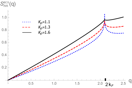
Figure 13: The density structure function $S^{\mbox{\tiny BCS}}_{nn}(q)$ for the BCS state for different interactions: $K_{\rho}=1.1$ (dotted blue), $K_{\rho}=1.3$ (dashed red) and $K_{\rho}=1.6$ (solid black). A pronounced cusp appears at $q=2k_{F}$.

For BCS state, the average magnetization is zero, but the magnetization-magnetization correlation does exhibit characteristic signatures,

$$\begin{split}S^{\mbox{\tiny BCS}}_{mm}(x)\sim-\cos(2k_{F}x)\left(\frac{a}{x}\right)^{K_{\rho}},\end{split}$$ (63)

with the corresponding magnetization structure function

$$\begin{split}S^{\mbox{\tiny BCS}}_{mm}(q)&\sim-\sqrt{\frac{2}{\pi}}\Gamma(1-K_{\rho})\sin(\pi K_{\rho}/2)\\ &\quad\times\left({|q-2k_{F}|^{K_{\rho}-1}}+{|q+2k_{F}|^{K_{\rho}-1}}\right),\end{split}$$ (64)

illustrated in Fig. 14.

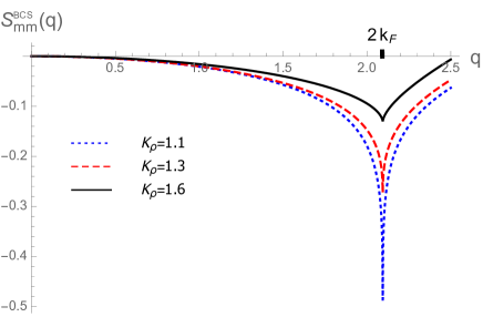
Figure 14: The magnetic structure function $S^{\mbox{\tiny BCS}}_{mm}(q)$ for the BCS state for different interactions: $K_{\rho}=1.1$ (dotted blue), $K_{\rho}=1.3$ (dashed red), and $K_{\rho}=1.6$ (solid black). An inverted characteristic cusp appears at $q=2k_{F}$.

VI.2 Spin-incommensurate state: FFLO

For $h>h_{c}=\Delta=U/\pi$, the strong Zeeman field exceeds spin-gap and the ground state becomes unstable to soliton proliferation in the bulk, leading to the FFLO. The spin-singlet pairing correlator is thus given by

$$\begin{split}S^{\mbox{\tiny FFLO}}_{ss}(x)&\sim\left(\frac{a}{x}\right)^{1/K_{\rho}+\kappa/2}\cos(k_{FFLO}x),\end{split}$$ (65)

with $k_{FFLO}=\pi\bar{m}=k_{F\uparrow}-k_{F\downarrow}$. While correlations still decay as a power-law, they also exhibit an oscillatory nonzero-momentum signature of the FFLO state. The associated exponent falls into a range $1<\eta^{\prime}\equiv K^{-1}_{\rho}+\kappa/2<2$ with the upper bound and lower bounds reached for $U\to 0$ and $U\to\infty$, respectively. The pairing correlations are thus in a range intermediate between fully paired BCS and unpaired fermions. This is consistent with the idea that FFLO is an intermediate “mixed” Zeeman-field ground state (given that FFLO is a compromise between the BCS and the unpaired state), analogous to the Abrikosov lattice of type-II superconductors.

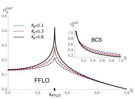
Figure 15: The Cooper-pair momentum distribution function in the FFLO ground state for $K_{\rho}=1.1$ (dotted blue), $K_{\rho}=1.3$ (dashed red), and $K_{\rho}=1.6$ (solid black) displaying a nonzero momentum $q=k_{FFLO}$ peak, narrowing with increasing interaction. Inset: The Cooper-pair momentum distribution for the BCS state, with a peak at zero-momentum.

The corresponding pair-momentum distribution function is then given by

$$\begin{split}n^{pair}_{q}&\sim\frac{\Gamma(1-\eta^{\prime})\sin(\pi\eta^{\prime}/2)}{\sqrt{2\pi}}\\ &\quad\times\left(|q-k_{FFLO}|^{\eta^{\prime}-1}+|q+k_{FFLO}|^{\eta^{\prime}-1}\right)\end{split}$$ (66)

is plotted in Fig. 15. In contrast with the spin-gapped BCS state, in the FFLO state the momentum distribution exhibits a peak at finite momentum $q=k_{FFLO}=k_{F\uparrow}-k_{F\downarrow}$, that sharpens as the interaction increases. This is also consistent with the numerical result reported in Feiguin07

The triplet-pairing correlator in the FFLO state is given by

$$\begin{split}S^{\mbox{\tiny FFLO}}_{st}(x)&\sim\left(\frac{a}{x}\right)^{1/K_{\rho}+2/\kappa},\end{split}$$ (67)

also decaying as a power-law. This is in sharp contrast with the BCS case where triplet pairing is exponentially suppressed. Since $1<\kappa<2$ (based on our discussion in Sec. V), $2/\kappa>\kappa/2$, indicating that in the FFLO ground state, triplet correlations are subdominant to the singlet ones (see Eq. (65) and Eq. (67)).

The density-density correlator in the FFLO state is given by

$$\begin{split}S^{\mbox{\tiny FFLO}}_{nn}(x)&\sim-K_{\rho}\left(\frac{a}{x}\right)^{2}\\ &\quad+\frac{1}{2}\left[\cos(2k_{F\uparrow}x)+\cos(2k_{F\downarrow}x)\right]\left(\frac{a}{x}\right)^{K_{\rho}+\kappa/2},\end{split}$$ (68)

with a two-component Friedel oscillations reflecting two fermionic populations, $2k_{F\uparrow,\downarrow}$.

The corresponding structure factor,

$$\begin{split}S^{\mbox{\tiny FFLO}}_{nn}(q)&\sim K_{\rho}\sqrt{\frac{\pi}{2}}|q|+\frac{\Gamma(1-\gamma)\sin(\pi\gamma/2)}{2\sqrt{2\pi}}({|q-2k_{F\uparrow}|^{\gamma-1}}\\ &\quad+{|q+2k_{F\uparrow}|^{\gamma-1}}+{|q+2k_{F\downarrow}|^{\gamma-1}}+{|q-2k_{F\downarrow}|^{\gamma-1}})\end{split}$$ (69)

where $\gamma\equiv K_{\rho}+\kappa/2>1$, is plotted in Fig. 16 for small magnetization $\bar{m}=\pi/10$, with $\kappa\sim 1$ according to Eq. (56). It displays cusps at $2k_{F\uparrow}$ and $2k_{F\downarrow}$, reflecting the contribution from pseudo-spin-up and pseudo-spin-down fermions, respectively and in a qualitative agreement with the DMRG results Rizzi .

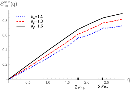
Figure 16: The density structure function $S^{\mbox{\tiny FFLO}}_{nn}(q)$ for the FFLO state for different interactions: $K_{\rho}=1.1$ (dotted blue), $K_{\rho}=1.3$ (dashed red) and $K_{\rho}=1.6$ (solid black), displaying cusps at $2k_{F\uparrow}$ and $2k_{F\downarrow}$, that reflect pseudo-spin-imbalance.

In the FFLO state the average magnetization density is uniform $\langle\hat{m}(x)\rangle=\bar{m}$, as the structure is washed out by strong quantum fluctuations in one dimension, that precludes spontaneous translational symmetry breaking. The characteristic short-scale correlations are captured by the magnetization-magnetization correlator

$$\begin{split}S^{\mbox{\tiny FFLO}}_{mm}(x)&\sim-\frac{\kappa}{2}\left(\frac{a}{x}\right)^{2}\\ &\quad-\frac{1}{2}\left[\cos(2k_{F\uparrow}x)+\cos(2k_{F\downarrow}x)\right]\left(\frac{a}{x}\right)^{K_{\rho}+\kappa/2},\end{split}$$ (70)

that distinguishes FFLO from the BCS state. The corresponding magnetic structure function is then given by

$$\begin{split}S^{\mbox{\tiny FFLO}}_{mm}(q)&\sim\frac{\kappa}{2}\sqrt{\frac{\pi}{2}}|q|-\frac{\Gamma(1-\gamma)\sin(\pi\gamma/2)}{2\sqrt{2\pi}}\Big{(}{|q-2k_{F\uparrow}|^{\gamma-1}}\\ &+{|q+2k_{F\uparrow}|^{\gamma-1}}+{|q+2k_{F\downarrow}|^{\gamma-1}}+{|q-2k_{F\downarrow}|^{\gamma-1}}\Big{)}\end{split}$$ (71)

and is illustrated in Fig. 17.

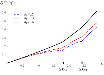
Figure 17: The magnetic structure function $S^{\mbox{\tiny FFLO}}_{mm}(q)$ for the FFLO state for different interactions: $K_{\rho}=1.1$ (dotted blue), $K_{\rho}=1.3$ (dashed red) and $K_{\rho}=1.6$ (solid black).

The above analysis thus demonstrates that there are clear qualitative features that distinguish the BCS and the FFLO ground states, even in the presence of strong quantum fluctuations.

VII quench dynamics: charge sector

We now turn to the nonequilibrium dynamics following a quantum quench for the 1D Hubbard model. We first study the quench dynamics of the charge sector (10). Here we consider a generic quench protocol of a sudden shift of the Luttinger parameter $K_{\rho}$ from $K_{\rho 0}$ to $K_{\rho 1}$, induced by the corresponding quench of the interaction $U$ possible in Feshbach resonant systems. The quadratic form of the charge sector Hamiltonian lends itself to an exact analysis, as has been done in a variety of systems CazalillaPRA ; Mitra2 ; HungChin13 ; NatuMueller13 ; Yin1 ; Cardy2 .

VII.1 Normal modes approach

As discussed in Sec. III, the pre-quench and post-quench Hamiltonians can be diagonalized by the following Bogoliubov transformations,

$$\begin{split}\begin{pmatrix}\hat{b}_{p}\\ \hat{b}^{\dagger}_{-p}\end{pmatrix}=\begin{pmatrix}\cosh\beta_{0}&-\sinh\beta_{0}\\ -\sinh\beta_{0}&\cosh\beta_{0}\end{pmatrix}\begin{pmatrix}\hat{\chi}_{p}\\ \hat{\chi}^{\dagger}_{-p}\end{pmatrix}\equiv U(0^{-})\begin{pmatrix}\hat{\chi}_{p}\\ \hat{\chi}^{\dagger}_{-p}\end{pmatrix},\end{split}$$ (72)

and

$$\begin{split}\begin{pmatrix}\hat{b}_{p}\\ \hat{b}^{\dagger}_{-p}\end{pmatrix}=\begin{pmatrix}\cosh\beta_{1}&-\sinh\beta_{1}\\ -\sinh\beta_{1}&\cosh\beta_{1}\end{pmatrix}\begin{pmatrix}\hat{\gamma}_{p}\\ \hat{\gamma}^{\dagger}_{-p}\end{pmatrix}\equiv U(0^{+})\begin{pmatrix}\hat{\gamma}_{p}\\ \hat{\gamma}^{\dagger}_{-p}\end{pmatrix},\end{split}$$ (73)

where ($\hat{\chi}^{\dagger}_{p},\hat{\chi}_{p}$) and ($\hat{\gamma}^{\dagger}_{p},\hat{\gamma}_{p}$) are the two sets of Bogoliubov quasiparticles, carrying momentum $p$. The parameters $\beta_{0}$ and $\beta_{1}$ are implicitly given by $e^{-2\beta_{0}}=K_{\rho 0}$ and $e^{-2\beta_{1}}=K_{\rho 1}$.

The charge sector dynamics after the quench ($t>0$) is thus given by

$$\begin{split}\begin{pmatrix}\hat{\gamma}_{p}(t)\\ \hat{\gamma}^{\dagger}_{-p}(t)\end{pmatrix}=\begin{pmatrix}e^{iv_{\rho 1}|p|t}&0\\ 0&e^{-iv_{\rho 1}|p|t}\end{pmatrix}\begin{pmatrix}\hat{\gamma}_{p}\\ \hat{\gamma}^{\dagger}_{-p}\end{pmatrix}\equiv U_{T}(t)\begin{pmatrix}\hat{\gamma}_{p}\\ \hat{\gamma}^{\dagger}_{-p}\end{pmatrix},\end{split}$$ (74)

where $v_{\rho 1}$ is the charge velocity for the post-quench Hamiltonian and $\hat{\gamma}_{p}\equiv\hat{\gamma}_{p}(t=0)$ and $\hat{\gamma}^{\dagger}_{p}\equiv\hat{\gamma}^{\dagger}_{p}(t=0)$.

Combining Eqs. (72), (73), and (74) relates ($\hat{b}^{\dagger}_{p}(t),\hat{b}_{-p}(t)$) to the initial pre-quench set of quasi-particles ($\hat{\chi}_{p},\hat{\chi}^{\dagger}_{-p}$) via

$$\begin{split}\begin{bmatrix}\hat{b}_{p}(t)\\ \hat{b}^{\dagger}_{-p}(t)\\ \end{bmatrix}&=U(0^{+})U_{T}(t)U^{-1}(0^{+})U(0^{-})\begin{bmatrix}\hat{\chi}_{p}\\ \hat{\chi}^{\dagger}_{-p}\\ \end{bmatrix},\end{split}$$ (75)

where the zero-temperature initial ground-state distribution of ($\hat{\chi}^{\dagger}_{p}$, $\hat{\chi}_{p}$) is given by $\langle\hat{\chi}_{p}\hat{\chi}^{\dagger}_{p^{\prime}}\rangle=\delta_{p,{p^{\prime}}}$.

The post-quench correlators of ${\hat{\phi}}_{\rho}(t)$ and ${\hat{\theta}}_{\rho}(t)$ can now be readily computed. Combining Eqs. (19) and (75), and relegating the details to Appendix C, we find

$$\begin{split}&\quad\langle e^{i\sqrt{2}[{\hat{\phi}}_{\rho}(x,t)-{\hat{\phi}}_{\rho}(0,t)}\rangle\\ &\sim\left(\frac{a}{x}\right)^{\frac{1}{2}(\frac{K^{2}_{\rho 1}}{K_{\rho 0}}+K_{\rho 0})}\left|\frac{x^{2}-(2v_{\rho 1}t)^{2}}{(2v_{\rho 1}t)^{2}+a^{2}}\right|^{\frac{1}{4}(\frac{K^{2}_{\rho 1}}{K_{\rho 0}}-K_{\rho 0})},\\ &\sim\begin{cases}\left(\frac{a}{x}\right)^{K_{\rho 0}}\left(\frac{1}{(2v_{\rho 1}t/a)^{2}+1}\right)^{\frac{1}{4}(\frac{K^{2}_{\rho 1}}{K_{\rho 0}}-K_{\rho 0})},&x\gg 2v_{\rho 1}t,\\ \left(\frac{a}{x}\right)^{\frac{1}{2}(K_{\rho 0}+\frac{K^{2}_{\rho 1}}{K_{\rho 0}})},&x\ll 2v_{\rho 1}t,\end{cases}\end{split}$$ (76)

$$\begin{split}&\quad\langle e^{i\sqrt{2}[{\hat{\theta}}_{\rho}(x,t)-{\hat{\theta}}_{\rho}(0,t)}\rangle\\ &\sim\left(\frac{a}{x}\right)^{\frac{1}{2}(\frac{K_{\rho 0}}{K^{2}_{\rho 1}}+\frac{1}{K_{\rho 0}})}\left|\frac{x^{2}-(2v_{\rho 1}t)^{2}}{(2v_{\rho 1}t)^{2}+a^{2}}\right|^{\frac{1}{4}(\frac{K_{\rho 0}}{K^{2}_{\rho 1}}-\frac{1}{K_{\rho 0}})},\\ &\sim\begin{cases}\left(\frac{a}{x}\right)^{K^{-1}_{\rho 0}}\left(\frac{1}{(2v_{\rho 1}t/a)^{2}+1}\right)^{\frac{1}{4}(\frac{K_{\rho 0}}{K^{2}_{\rho 1}}-\frac{1}{K_{\rho 0}})},&x\gg 2v_{\rho 1}t,\\ \left(\frac{a}{x}\right)^{\frac{1}{2}(\frac{K_{\rho 0}}{K^{2}_{\rho 1}}+\frac{1}{K_{\rho 0}})},&x\ll 2v_{\rho 1}t,\end{cases}\end{split}$$ (77)

and

$$\begin{split}&\quad 2a^{2}\langle\partial_{x}{\hat{\phi}}_{\rho}(x,t)\partial_{x^{\prime}}{\hat{\phi}}_{\rho}(0,t)\rangle\\ &=-\frac{(K_{\rho 0}+\frac{K^{2}_{\rho 1}}{K_{\rho 0}})a^{2}}{2x^{2}}-\frac{(K_{\rho 0}-\frac{K^{2}_{\rho 1}}{K_{\rho 0}})a^{2}}{4(x+2v_{\rho 1}t)^{2}}-\frac{(K_{\rho 0}-\frac{K^{2}_{\rho 1}}{K_{\rho 0}})a^{2}}{4(x-2v_{\rho 1}t)^{2}}.\end{split}$$ (78)

We will combine these dynamical charge sector correlators with the spin sector ones to calculate observables for the Hubbard model, as we have done earlier for the equilibrium case. However, before moving on we will reproduce above charge correlators using a simpler approach, that will be essential for the spin sector analysis, where the nonlinearity precludes a direct diagonalization utilized above.

VII.2 Heisenberg equations of motion approach

A complementary approach to the above momentum eigenmodes Hamiltonian diagonalization is to directly solve the Heisenberg equation of motion for the field operators ${\hat{\phi}}_{\rho}(x,t)$ and ${\hat{\theta}}_{\rho}(x,t)$ in terms of the corresponding pre-quench operators, ${\hat{\phi}}_{\rho}(x,t=0)$ and ${\hat{\theta}}_{\rho}(x,t=0)$, whose correlators we have already computed in Sec. III.

Using the charge sector Hamiltonian (10) and the commutation relations,

$$\begin{split}[{\hat{\phi}}_{\rho}(x),\partial_{x^{\prime}}{\hat{\theta}}_{\rho}(x^{\prime})]=i\pi\delta(x-x^{\prime}),\\ [{\hat{\theta}}_{\rho}(x),\partial_{x^{\prime}}{\hat{\phi}}_{\rho}(x^{\prime})]=i\pi\delta(x-x^{\prime}),\end{split}$$ (79)

the coupled Heisenberg equations of motion for ${\hat{\phi}}_{\rho}$ and ${\hat{\theta}}_{\rho}$ are readily obtained:

$$\begin{split}\dot{\hat{\phi}}_{\rho}(x,t)&=K_{\rho 1}v_{\rho 1}\partial_{x}{\hat{\theta}}_{\rho}(x,t),\\ \dot{\hat{\theta}}_{\rho}(x,t)&=\frac{v_{\rho 1}}{K_{\rho 1}}\partial_{x}{\hat{\phi}}_{\rho}(x,t).\end{split}$$ (80)

As usual, they can be decoupled into wave equations:

$$\begin{split}\ddot{\hat{\phi}}_{\rho}(x,t)=v^{2}_{\rho 1}\partial^{2}_{x}{\hat{\phi}}_{\rho}(x,t),\\ \ddot{\hat{\theta}}_{\rho}(x,t)=v^{2}_{\rho 1}\partial^{2}_{x}{\hat{\theta}}_{\rho}(x,t),\end{split}$$ (81)

with the initial conditions

$$\begin{split}{\hat{\phi}}_{\rho}(x,0)&\equiv{\hat{\phi}}_{\rho}(x),\\ {\hat{\theta}}_{\rho}(x,0)&\equiv{\hat{\theta}}_{\rho}(x),\\ \dot{\hat{\phi}}_{\rho}(x,0)&=K_{\rho 1}v_{\rho 1}\partial_{x}{\hat{\theta}}_{\rho},\\ \dot{\hat{\theta}}_{\rho}(x,0)&=\frac{v_{\rho 1}}{K_{\rho 1}}\partial_{x}{\hat{\phi}}_{\rho}.\end{split}$$ (82)

The dynamics is now straightforwardly obtained as a linear combination of the left and right traveling solutions satisfying the above initial conditions,

$${\hat{\phi}}_{\rho}(x,t) =\frac{1}{2}[{\hat{\phi}}_{\rho}(x+v_{\rho 1}t)+{\hat{\phi}}_{\rho}(x-v_{\rho 1}t)]$$

$$\quad+\frac{K_{\rho 1}}{2}[{\hat{\theta}}_{\rho}(x+v_{\rho 1}t)-{\hat{\theta}}_{\rho}(x-v_{\rho 1}t)],$$ (83a)

$${\hat{\theta}}_{\rho}(x,t) =\frac{1}{2}[{\hat{\theta}}_{\rho}(x+v_{\rho 1}t)+{\hat{\theta}}_{\rho}(x-v_{\rho 1}t)]$$

$$\quad+\frac{1}{2K_{\rho 1}}[{\hat{\phi}}_{\rho}(x+v_{\rho 1}t)-{\hat{\phi}}_{\rho}(x-v_{\rho 1}t)],$$ (83b)

with operators at $t=0$ appearing on the right-hand side. These thus allow us to connect the post-quench dynamical correlators (with all averages taken in the pre-quenched initial ground state) to their initial $t=0^{-}$ pre-quench counterparts,

$$\begin{split}&\quad\langle e^{i\sqrt{2}[{\hat{\phi}}_{\rho}(x,t)-{\hat{\phi}}_{\rho}(0,t)]}\rangle\\ &=\langle e^{i\frac{\sqrt{2}}{2}[{\hat{\phi}}_{\rho}(x+v_{\rho 1}t)+{\hat{\phi}}_{\rho}(x-v_{\rho 1}t)-{\hat{\phi}}_{\rho}(v_{\rho 1}t)-{\hat{\phi}}_{\rho}(-v_{\rho 1}t)]}\rangle\\ &\quad\times\langle e^{i\frac{\sqrt{2}K_{\rho 1}}{2}[{\hat{\theta}}_{\rho}(x+v_{\rho 1}t)-{\hat{\theta}}_{\rho}(x-v_{\rho 1}t)-{\hat{\theta}}_{\rho}(v_{\rho 1}t)+{\hat{\theta}}_{\rho}(-v_{\rho 1}t)]}\rangle,\\ &=e^{1/4[2F_{\hat{\phi}}(2v_{\rho 1}t)-2F_{\hat{\phi}}(x)-F_{\hat{\phi}}(x+2v_{\rho 1}t)-F_{\hat{\phi}}(|x-2v_{\rho 1}t|)]}\\ &\quad\times e^{-K^{2}_{\rho 1}/4[2F_{\hat{\theta}}(2v_{\rho 1}t)+2F_{\hat{\theta}}(x)-F_{\hat{\theta}}(x+2v_{\rho 1}t)-F_{\hat{\theta}}(|x-2v_{\rho 1}t|)]},\end{split}$$ (84)

and

$$\begin{split}&\quad\langle e^{i\sqrt{2}[{\hat{\theta}}_{\rho}(x,t)-{\hat{\theta}}_{\rho}(0,t)}\rangle\\ &=\langle e^{i\frac{\sqrt{2}}{2}[{\hat{\theta}}_{\rho}(x+v_{\rho 1}t)+{\hat{\theta}}_{\rho}(x-v_{\rho 1}t)-{\hat{\theta}}_{\rho}(v_{\rho 1}t)-{\hat{\theta}}_{\rho}(-v_{\rho 1}t)]}\rangle\\ &\quad\times\langle e^{i\frac{\sqrt{2}}{2K_{\rho 1}}[{\hat{\phi}}_{\rho}(x+v_{\rho 1}t)-{\hat{\phi}}_{\rho}(x-v_{\rho 1}t)-{\hat{\phi}}_{\rho}(v_{\rho 1}t)+{\hat{\phi}}_{\rho}(-v_{\rho 1}t)]}\rangle,\\ &=e^{1/4[2F_{\hat{\theta}}(2v_{\rho 1}t)-2F_{\hat{\theta}}(x)-F_{\hat{\theta}}(x+2v_{\rho 1}t)-F_{\hat{\theta}}(|x-2v_{\rho 1}t|)]}\\ &\quad\times e^{-1/(4K^{2}_{\rho 1})[2F_{\hat{\phi}}(2v_{\rho 1}t)+2F_{\hat{\phi}}(x)-F_{\hat{\phi}}(x+2v_{\rho 1}t)-F_{\hat{\phi}}(|x-2v_{\rho 1}t|)]},\end{split}$$ (85)

with the details evaluated in Appendix E. Using the initial pre-quench correlators of ${\hat{\phi}}_{\rho}(x)$ and ${\hat{\theta}}_{\rho}(x)$, studied in Sec. III,

$$\begin{split}F_{\hat{\phi}}(x)&\equiv\langle({\hat{\phi}}_{\rho}(x)-{\hat{\phi}}_{\rho}(0))^{2}\rangle\sim K_{\rho 0}\ln\frac{x}{a},\\ F_{\hat{\theta}}(x)&\equiv\langle({\hat{\theta}}_{\rho}(x)-{\hat{\theta}}_{\rho}(0))^{2}\rangle\sim\frac{1}{K_{\rho 0}}\ln\frac{x}{a}.\end{split}$$ (86)

inside Eqs. (84) and (85), we much more simply reproduce the results (LABEL:quenchluttingerphitheta) and (LABEL:quenchluttingerphitheta2) obtained with the Hamiltonian diagonalization approach.

VIII Quench dynamics of spin sector

We now study the dynamics of the spin sector Hamiltonian (11) following a $U\to 0$ quench to noninteracting fermions at $t=0$. This quench protocol is simple enough to be conveniently implemented in experiments, yet still contains the essential elements of the nonequilibrium dynamics. It also has the appeal that the post-quench evolution is exactly solvable, reducing all the difficulties to the analysis of correlations in the initial interacting state.

Thus for the $U\to 0$ quench protocol, the Heisenberg equations of motion satisfied by ${\hat{\phi}}_{\sigma}(x,t)$ and ${\hat{\theta}}_{\sigma}(x,t)$ is still a linear wave equation (81) with initial conditions

$$\begin{split}{\hat{\phi}}_{\sigma}(x,0)&\equiv{\hat{\phi}}_{\sigma}(x),\\ {\hat{\theta}}_{\sigma}(x,0)&\equiv{\hat{\theta}}_{\sigma}(x),\\ \dot{\hat{\phi}}_{\sigma}(x,0)&=v_{F}\partial_{x}{\hat{\theta}}_{\sigma},\\ \dot{\hat{\theta}}_{\sigma}(x,0)&=v_{F}\partial_{x}{\hat{\phi}}_{\sigma}+\frac{\sqrt{2}h}{\pi}.\end{split}$$ (87)

and the post-quench Luttinger parameters $K_{\sigma}=1$ and $v_{\sigma}=v_{F}$ for free fermions.

The solution thus is straightforwardly obtained and is quite similar to the charge sector,

$${\hat{\phi}}_{\sigma}(x,t) =\frac{1}{2}[{\hat{\phi}}_{\sigma}(x+v_{F}t)+{\hat{\phi}}_{\sigma}(x-v_{F}t)]$$

$$\quad+\frac{1}{2}[{\hat{\theta}}_{\sigma}(x+v_{F}t)-{\hat{\theta}}_{\sigma}(x-v_{F}t)],$$ (88a)

$${\hat{\theta}}_{\sigma}(x,t) =\frac{1}{2}[{\hat{\theta}}_{\sigma}(x+v_{F}t)+{\hat{\theta}}_{\sigma}(x-v_{F}t)]$$

$$\quad+\frac{1}{2}[{\hat{\phi}}_{\sigma}(x+v_{F}t)-{\hat{\phi}}_{\sigma}(x-v_{F}t)]+\frac{\sqrt{2}h}{\pi}t.$$ (88b)

The dynamical correlators at time $t$ can then again be expressed in terms of the pre-quench ones at the initial time,

$$\begin{split}&\quad\langle e^{i\sqrt{2}[{\hat{\phi}}_{\sigma}(x,t)-{\hat{\phi}}_{\sigma}(0,t)}\rangle\\ &=e^{1/4[2D_{\hat{\phi}}(2v_{F}t)-2D_{\hat{\phi}}(x)-D_{\hat{\phi}}(x+2v_{F}t)-D_{\hat{\phi}}(|x-2v_{F}t|)]}\\ &\quad\times e^{-1/4[2D_{\hat{\theta}}(2v_{F}t)+2D_{\hat{\theta}}(x)-D_{\hat{\theta}}(x+2v_{F}t)-D_{\hat{\theta}}(|x-2v_{F}t|)]},\end{split}$$ (89)

and

$$\begin{split}&\quad\langle e^{i\sqrt{2}[{\hat{\theta}}_{\sigma}(x,t)-{\hat{\theta}}_{\sigma}(0,t)}\rangle\\ &=e^{1/4[2D_{\hat{\theta}}(2v_{F}t)-2D_{\hat{\theta}}(x)-D_{\hat{\theta}}(x+2v_{F}t)-D_{\hat{\theta}}(|x-2v_{F}t|)]}\\ &\quad\times e^{-1/4[2D_{\hat{\phi}}(2v_{F}t)+2D_{\hat{\phi}}(x)-D_{\hat{\phi}}(x+2v_{F}t)-D_{\hat{\phi}}(|x-2v_{F}t|)]},\end{split}$$ (90)

where

$$\begin{split}D_{\hat{\phi}}(x)&\equiv\langle({\hat{\phi}}_{\sigma}(x)-{\hat{\phi}}_{\sigma}(0))^{2}\rangle,\\ D_{\hat{\theta}}(x)&\equiv\langle({\hat{\theta}}_{\sigma}(x)-{\hat{\theta}}_{\sigma}(0))^{2}\rangle\end{split}$$ (91)

are the correlators for ${\hat{\phi}}_{\sigma}(x)$ and ${\hat{\theta}}_{\sigma}(x)$ prior to the quench. These depend qualitatively on the initial state, as we now discuss for quenches from the BCS and the FFLO ground states.

VIII.1 Quench $U\to 0$ from BCS state

Following the quench from the BCS state to the non-interacting Fermi gas, the classical field part $\langle{\hat{\phi}}_{\sigma}(x,t)\rangle$ evolves according to Eq. (88), given approximately by

$$\begin{split}&\langle{\hat{\phi}}_{\sigma}(x,t)\rangle=\frac{1}{2}[\langle{\hat{\phi}}_{\sigma}(x+v_{F}t)\rangle+\langle{\hat{\phi}}_{\sigma}(x-v_{F}t)\rangle]\\ &\sim\begin{cases}0,&|x|<L/2-\xi^{\prime}-v_{F}t,\\ h\frac{\sqrt{2K_{\sigma}}}{4\pi}\left(x-L/2+\xi^{\prime}+v_{F}t\right),&|x|>L/2-\xi^{\prime}-v_{F}t.\end{cases}\end{split}$$ (92)

This describes the penetration of magnetization into the bulk via a ballistic motion of a fraction of a soliton from the edge into the bulk, and as expected eventually leads to a constant magnetization (species imbalance) of the noninteracting Fermi gas in the presence of a finite Zeeman field (chemical potential imbalance) $h$. However, this takes a macroscopically long time $t_{L}\approx L/v_{F}$ to travel through the system. From here on, we will focus on the thermodynamic limit ($L\rightarrow\infty$ but $t$ finite), in the bulk of the sample and thus neglect these “edge” effects. We will thus take $\langle{\hat{\phi}}_{\sigma}(x,t)\rangle=0$ in the spin-gapped BCS ground state.

Using the BCS ground-state correlators from Sec. V,

$$\begin{split}D^{\mbox{\tiny BCS}}_{\hat{\phi}}(x)&\sim\operatorname{const}.,\\ D^{\mbox{\tiny BCS}}_{\hat{\theta}}(x)&\sim x/\xi+\operatorname{const}.\end{split}$$ (93)

inside post-quench ones at time $t$, Eq. (89),(90), we obtain

$$\begin{split}\langle e^{i\sqrt{2}[{\hat{\phi}}_{\sigma}(x,t)-{\hat{\phi}}_{\sigma}(0,t)}\rangle&\sim e^{-(x+2v_{F}t-|x-2v_{F}t|)/(4\xi)}\\ &\sim\begin{cases}e^{-\frac{2v_{F}t}{2\xi}},&x\gg 2v_{F}t,\\ e^{-\frac{x}{2\xi}},&x\ll 2v_{F}t,\end{cases}\end{split}$$ (94)

and

$$\begin{split}\langle e^{i\sqrt{2}[{\hat{\theta}}_{\sigma}(x,t)-{\hat{\theta}}_{\sigma}(0,t)}\rangle&\sim e^{-(3x+|x-2v_{F}t|-2v_{F}t)/(4\xi_{0})}\\ &\sim\begin{cases}e^{-\frac{x-v_{F}t}{\xi}},&x\gg 2v_{F}t,\\ e^{-\frac{x}{2\xi}},&x\ll 2v_{F}t,\end{cases}\end{split}$$ (95)

These exhibit exponential behavior in time and space and at long time reach a stationary form. As we will see these differ qualitatively from a quench from the FFLO state to which we turn next.

VIII.2 Quench $U\to 0$ from FFLO state

The nonzero magnetization in the FFLO state is carried by a soliton lattice. Thus, following a quench we expect nontrivial dynamics associated with soliton lattice oscillations and breathing, described by the solution of the sine-Gordon equation. However, strong 1D quantum fluctuations wash out this classical dynamics, that will, however, appear in higher dimensions. Furthermore, as we have seen in Sec. V, outside of a narrow range above $h_{c}$ solitons strongly overlap, leading to a vanishing periodic (in space) component of the density. The magnetization can therefore be well approximated by a constant, corresponding to

$$\begin{split}\langle{\hat{\phi}}_{\sigma}(x,t)\rangle&\sim\frac{\pi\bar{m}}{\sqrt{2}}x.\end{split}$$ (96)

Recalling from Sec. V, the FFLO ground state pre-quench correlations are given by

$$\begin{split}D^{\mbox{\tiny FFLO}}_{\hat{\phi}}(x)&=1/2\langle(\tilde{\phi}_{\sigma}(x)-\tilde{\phi}_{\sigma}(0))^{2}\rangle\sim\frac{\kappa}{2}\ln\frac{x}{a},\\ D^{\mbox{\tiny FFLO}}_{\hat{\theta}}(x)&=2\langle(\tilde{\theta}_{\sigma}(x)-\tilde{\theta}_{\sigma}(0))^{2}\rangle\sim\frac{2}{\kappa}\ln\frac{x}{a}.\end{split}$$ (97)

Using them inside post-quench correlators in Eqs. (89) and (90), we find

$$\begin{split}\langle e^{i\sqrt{2}[{\hat{\phi}}_{\rho}(x,t)-{\hat{\phi}}_{\rho}(0,t)}\rangle&\sim e^{i\pi\bar{m}x}\left(\frac{a}{x}\right)^{\frac{1}{2}(\frac{2}{\kappa}+\frac{\kappa}{2})}\\ &\quad\times\left|\frac{x^{2}-(2v_{F}t)^{2}}{(2v_{F}t)^{2}+a^{2}}\right|^{\frac{1}{4}(\frac{2}{\kappa}-\frac{\kappa}{2})},\end{split}$$ (98)

$$\begin{split}\langle e^{i\sqrt{2}[{\hat{\theta}}_{\rho}(x,t)-{\hat{\theta}}_{\rho}(0,t)}\rangle&\sim\left(\frac{a}{x}\right)^{\frac{1}{2}(\frac{2}{\kappa}+\frac{\kappa}{2})}\left|\frac{(2v_{F}t)^{2}+a^{2}}{x^{2}-(2v_{F}t)^{2}}\right|^{\frac{1}{4}(\frac{2}{\kappa}-\frac{\kappa}{2})},\end{split}$$ (99)

and

$$\begin{split}&\quad 2a^{2}\langle\partial_{x}{\hat{\phi}}_{\sigma}(x)\partial_{x^{\prime}}{\hat{\phi}}_{\sigma}(0)\rangle\\ &\sim-\frac{(\kappa/2+2/\kappa)a^{2}}{2x^{2}}-\frac{(\kappa/2-2/\kappa)a^{2}}{4(x+2v_{F}t)^{2}}-\frac{(\kappa/2-2/\kappa)a^{2}}{4(x-2v_{F}t)^{2}}.\end{split}$$ (100)

These power-law dynamic correlations contrast strongly with those for the quench from the BCS state and exhibit a long-time stationary pre-thermalized state.

IX 1D spin-imbalanced Fermi-Hubbard model: Quench dynamics

We now are in the position to assemble the results from earlier sections to predict the quench dynamics of the 1D spin-imbalanced Fermi gas, described by the Fermi-Hubbard model. As discussed in Sec. VIII, in this paper we limit our study to a quench protocol to a vanishing on-site interaction, i.e., a quench $U\to 0$. Such quench is not only simpler to analyze, but also more straightforwardly implementable in a Feshbach resonant gas by tuning to a point of a vanishing scattering length and by shutting off the trap.

IX.1 $U\to 0$ from BCS state

Combining Eqs. (LABEL:quenchluttingerphitheta2) and (94), we obtain the spin-singlet pairing correlator [defined via Eqs. (13a) and (16)] at time $t$, following a $U\rightarrow 0$ quench from an initial BCS ground state,

$$\begin{split}&\quad S^{\mbox{\tiny BCS}}_{ss}(x,t)\\ &=\langle e^{i\sqrt{2}[{\hat{\theta}}_{\rho}(x,t)-{\hat{\theta}}_{\rho}(0,t)]}\rangle\langle\cos(\sqrt{2}{\hat{\phi}}_{\sigma}(x,t))\cos(\sqrt{2}{\hat{\phi}}_{\sigma}(0,t))\rangle,\\ &\sim\left(\frac{a}{x}\right)^{(K_{\rho 0}+K^{-1}_{\rho 0})/2}\left|\frac{x^{2}-(2v_{F}t)^{2}}{(2v_{F}t)^{2}+a^{2}}\right|^{(K_{\rho 0}-K^{-1}_{\rho 0})/4}\\ &\quad\times e^{-(x+2v_{F}t-|x-2v_{F}t|)/(4\xi)},\\ &\sim\begin{cases}\left(\frac{a}{x}\right)^{K^{-1}_{\rho 0}}\left(\frac{a}{2v_{F}t}\right)^{(K_{\rho 0}-K^{-1}_{\rho 0})/2}e^{-\frac{v_{F}t}{\xi}},&x\gg 2v_{F}t,\\ \left(\frac{a}{x}\right)^{(K_{\rho 0}+K^{-1}_{\rho 0})/2}e^{-\frac{x}{2\xi}},&x\ll 2v_{F}t,\end{cases}\\ \end{split}$$ (101)

illustrated in Fig. 1 and Fig. 2. We observe that despite the initial power-law correlations in the BCS ground state (set by gapless charge fluctuations), at the light-cone time $t_{*}(x)=x/(2v_{F})$ Cardy , these correlations crossover to short-ranged stationary ones set by the correlation length $\xi$.

Above dynamics is also reflected in momentum space. We illustrate in Fig. 18 the spatial Fourier transform of $S^{\mbox{\tiny BCS}}_{ss}(x,t)$, namely the Cooper-pair momentum distribution $n^{pair}_{q}(t)$. We observe that the strength of zero-momentum peak decays in time, indicating the collapse of the BCS pairing following the quench to the noninteracting state. This is consistent with the exponentially decaying BCS pairing order shown in Eq. (101).

Figure 18: Cooper-pair momentum distribution $n^{pair}_{q}(t)$ for a series of time following the quantum quench $U\to 0$ at $t=0$ from the BCS ground state for $K_{\rho}=1.6$ at $t=0^{-}$. It illustrates a decay of the zero-momentum peak following the quench.

Figure 19: Space-time intensity plot of density-density correlation function $S^{\mbox{\tiny BCS}}_{nn}(q,t)$ following a $U\to 0$ quench at $t=0$ from the BCS state for $K_{\rho}=1.6$ at $t=0^{-}$. The light-cone boundary ($x=2v_{F}t$, the dotted line is a guide to an eye) is a crossover between the early-time ground-state correlation to those in the asymptotic long time stationary state.

Figure 20: Structure function $S^{\mbox{\tiny BCS}}_{nn}(q,t)$ for a series of time following the quantum quench $U\to 0$ at $t=0$ from the BCS spin-singlet ground state for $K_{\rho}=1.6$ at $t=0^{-}$, with approximate analytical form given by Eq. (104).

Combining Eqs. (LABEL:quenchluttingerphitheta2) and (95), we obtain the post-quench dynamical spin-triplet correlator (defined via Eq. (13b)(17))

$$\begin{split}&\quad S^{\mbox{\tiny BCS}}_{st}(x,t)\\ &=\langle e^{i\sqrt{2}[{\hat{\theta}}_{\rho}(x,t)-{\hat{\theta}}_{\rho}(0,t)]}\rangle\langle\cos(\sqrt{2}{\hat{\theta}}_{\sigma}(x,t))\cos(\sqrt{2}{\hat{\theta}}_{\sigma}(0,t))\rangle\\ &\sim\left(\frac{a}{x}\right)^{(K_{\rho 0}+K^{-1}_{\rho 0})/2}\left|\frac{x^{2}-(2v_{F}t)^{2}}{(2v_{F}t)^{2}+a^{2}}\right|^{(K_{\rho 0}-K^{-1}_{\rho 0})/4}\\ &\quad\times e^{-(3x+|x-2v_{F}t|-2v_{F}t)/(4\xi)},\\ &\sim\begin{cases}e^{-\frac{x-v_{F}t}{\xi}}\left(\frac{a}{x}\right)^{K^{-1}_{\rho 0}}\left(\frac{a}{2v_{F}t}\right)^{(K_{\rho 0}-K^{-1}_{\rho 0})/2},&x\gg 2v_{F}t,\\ e^{-\frac{x}{2\xi}}\left(\frac{a}{x}\right)^{(K_{\rho 0}+K^{-1}_{\rho 0})/2},&x\ll 2v_{F}t.\end{cases}\end{split}$$ (102)

We observe that it also displays a light-cone crossover from a spatial exponential decay in the singlet BCS ground state at short times to a stationary exponential decay with a doubled correlation length at long time $t>t_{*}(x)$. The doubled correlation length seems to indicate that, compared to the initial singlet BCS ground state, the triplet-pairing is enhanced as the former is exponentially suppressed.

Combining Eqs. (LABEL:quenchluttingerphitheta), (78), and (94) we obtain the post-quench density-density correlation function,

$$\begin{split}S^{\mbox{\tiny BCS}}_{nn}(x,t)&=2a^{2}\langle\partial_{x}{\hat{\phi}}_{\rho}(x,t)\partial_{x^{\prime}}{\hat{\phi}}_{\rho}(0,t)\rangle+e^{-2ik_{F}x}\langle e^{i\sqrt{2}[{\hat{\phi}}_{\rho}(x,t)-{\hat{\phi}}_{\rho}(0,t)}\rangle\langle\cos(\sqrt{2}{\hat{\phi}}_{\sigma}(x,t))\cos(\sqrt{2}{\hat{\phi}}_{\sigma}(0,t))\rangle+h.c.,\\ &\sim-\frac{{1}}{2}\left((K_{\rho 0}+K^{-1}_{\rho 0})\left|\frac{a}{x}\right|^{2}+\frac{K_{\rho 0}-K^{-1}_{\rho 0}}{2}\left[\frac{a^{2}}{(x+2v_{F}t)^{2}}+\frac{a^{2}}{(x-2v_{F}t)^{2}}\right]\right)\\ &\quad+\cos(2k_{F}x)\left(\frac{a}{x}\right)^{(K_{\rho 0}+K^{-1}_{\rho 0})/2}\left|\frac{(2v_{F}t)^{2}+a^{2}}{x^{2}-(2v_{F}t)^{2}}\right|^{(K_{\rho 0}-K^{-1}_{\rho 0})/4}e^{-(x+2v_{F}t-|x-2v_{F}t|)/(4\xi)}\\ &\sim\begin{cases}-K_{\rho 0}\left|\frac{a}{x}\right|^{2}+\left(\frac{a}{x}\right)^{K_{\rho 0}}\left(\frac{2v_{F}t}{a}\right)^{(K_{\rho 0}-K^{-1}_{\rho 0})/2}e^{-\frac{v_{F}t}{\xi}}\cos(2k_{F}x),&x\gg 2v_{F}t,\\ -\frac{1}{4}(K_{\rho 0}-K^{-1}_{\rho 0})\frac{a^{2}}{(x-2v_{F}t)^{2}},&x\approx 2v_{\sigma}t,\\ -\frac{1}{2}(K_{\rho 0}+K^{-1}_{\rho 0})\left|\frac{a}{x}\right|^{2}+\left(\frac{a}{x}\right)^{(K_{\rho 0}+K^{-1}_{\rho 0})/2}e^{-\frac{x}{2\xi}}\cos(2k_{F}x),&x\ll 2v_{\sigma}t.\end{cases}\end{split}$$ (103)

illustrated in Figs. 5 and 19. It displays a divergent power-law peak at the light-cone boundary $x=2v_{F}t$, instead of a moving light-cone node for the spin-singlet (101) and triplet (102) correlators. In the bulk, for early time ($t<t_{*}(x)$) the correlator displays spatial correlations of the initial ground state, with a time-dependent decaying pre-factor. In the long time limit ($t>t_{*}(x)$) it crosses over to a time-independent stationary form, expected for a pre-thermalized state.

The corresponding structure function $S^{\mbox{\tiny BCS}}_{nn}(q)$ is illustrated in Fig. 20. It displays a buildup of oscillations as time evolves. Noting from Eq. (103) that the charge sector contribution dominates over the spin sector, the structure function can be well approximated by

$$\begin{split}S^{\mbox{\tiny BCS}}_{nn}(q)&\sim\sqrt{\frac{\pi}{2}}|q|\left[(K_{\rho 0}+K^{-1}_{\rho 0})+(K_{\rho 0}-K^{-1}_{\rho 0})\cos(2qv_{F}t)\right]\end{split}$$ (104)

qualitatively consistent with the behavior of the full expression illustrated Fig. 20.

The dynamical magnetization-magnetization correlator is given by

$$\begin{split}&S^{\mbox{\tiny BCS}}_{mm}(x)=-\cos(2k_{F}x)\left(\frac{a}{x}\right)^{(K_{\rho 0}+K^{-1}_{\rho 0})/2}\\ &\quad\quad\times\left|\frac{(2v_{F}t)^{2}+a^{2}}{x^{2}-(2v_{F}t)^{2}}\right|^{(K_{\rho 0}-K^{-1}_{\rho 0})/4}e^{-(x+2v_{F}t-|x-2v_{F}t|)/(4\xi)}\\ &\sim\begin{cases}-\left(\frac{a}{x}\right)^{K_{\rho 0}}\left(\frac{2v_{F}t}{a}\right)^{(K_{\rho 0}-K^{-1}_{\rho 0})/2}e^{-\frac{v_{F}t}{\xi}}\cos(2k_{F}x),&x\gg 2v_{F}t,\\ -\left(\frac{a}{x}\right)^{(K_{\rho 0}+K^{-1}_{\rho 0})/2}e^{-\frac{x}{2\xi}}\cos(2k_{F}x),&x\ll 2v_{\sigma}t.\end{cases}\end{split}$$ (105)

It is illustrated in Figs. 21 and 22 and also shows light-cone dynamics and thermalization. The evolution is more evidently demonstrated in momentum space (see Fig. 23), where following the quench the $2k_{F}$ quasi-Bragg peak of the BCS ground state is suppressed and rounded into a Lorentzian following the quench.

Figure 21: Space-time intensity plot of the magnetization-magnetization correlation function $S^{\mbox{\tiny BCS}}_{mm}(x,t)$ following a $U\to 0$ quench at $t=0$ from the BCS state for $K_{\rho}=1.6$ at $t=0^{-}$. At the light-cone time $t_{*}(x)=x/(2v_{F})$, the correlation shows a crossover from the spatial dependence of the initial ground state to the one of the thermalized stationary state.

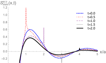
Figure 22: Magnetization-magnetization correlation function $S^{\mbox{\tiny BCS}}_{mm}(x,t)$ following a $U\to 0$ quench at $t=0$ from the BCS state for a series of times. The peak moves as a light-cone wave-front, $x=2v_{F}t$.

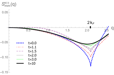
Figure 23: Magnetization structure function $S^{\mbox{\tiny BCS}}_{mm}(q,t)$ for a series of times following a $U\to 0$ quench at $t=0$ from the BCS state for $K_{\rho}=1.6$ at $t=0^{-}$. With time, the $2k_{F}$ peak evolves from the quasi-Bragg peak of the ground-state to a Lorentzian at long times.

IX.2 $U\to 0$ from FFLO state

Using results of previous sections, Eqs. (LABEL:quenchluttingerphitheta2) and (94) inside (16), we obtain the spin-singlet pairing correlator following a $U\rightarrow 0$ quench from an initial FFLO ground state,

$$\begin{split}S^{\mbox{\tiny FFLO}}_{ss}(x,t)&\sim\cos(k_{FFLO}x)\left(\frac{a}{x}\right)^{(\frac{\kappa}{2}+\frac{2}{\kappa}+K_{\rho 0}+K^{-1}_{\rho 0})/2}\left|\frac{x^{2}-(2v_{F}t)^{2}}{(2v_{F}t)^{2}+a^{2}}\right|^{\frac{1}{4}(K_{\rho 0}-K^{-1}_{\rho 0}+\frac{2}{\kappa}-\frac{\kappa}{2})},\\ &\sim\cos(k_{FFLO}x)\begin{cases}\left(\frac{a}{x}\right)^{K^{-1}_{\rho 0}+\frac{\kappa}{2}}\left(\frac{a}{2v_{F}t}\right)^{\frac{1}{2}(K_{\rho 0}-K^{-1}_{\rho 0}+\frac{2}{\kappa}-\frac{\kappa}{2})},&x\gg 2v_{F}t,\\ \left(\frac{a}{x}\right)^{\frac{1}{2}(\frac{\kappa}{2}+\frac{2}{\kappa}+K_{\rho 0}+K^{-1}_{\rho 0})},&x\ll 2v_{F}t.\end{cases}\end{split}$$ (106)

illustrated in Fig. 3 and 4. It displays a light-cone crossover from the early time ($t<t_{*}(x)$) spatial power-law correlations of the FFLO ground state to a long-time stationary shorter-range power-law correlations.

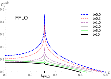
Figure 24: Cooper-pair momentum distribution $n^{pair}_{q}(t)$ for a series of time following the quantum quench $U\to 0$ at $t=0$ from the FFLO ground state for $K_{\rho}=1.6$ at $t=0^{-}$. The FFLO peak shrinks with increasing time following the quench.

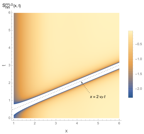
Figure 25: Space-time intensity plot of density-density correlation function $S^{\mbox{\tiny FFLO}}_{nn}(x,t)$ following a $U\to 0$ quench at $t=0$ from the FFLO state for $K_{\rho}=1.6$ at $t=0^{-}$. The light-cone boundary ($x=2v_{F}t$, the dotted line is a guidance to the eye) separates early-time ground-state correlation from those in the asymptotic large time stationary state.

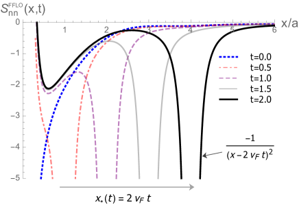
Figure 26: Density-density correlation function $S^{\mbox{\tiny FFLO}}_{nn}(x,t)$ following a $U\to 0$ quench at $t=0$ from the FFLO state for a series of times. The dominant features is the moving power-law peak $-1/(x-2v_{F}t)^{2}$ at the light-cone boundary, similar to the BCS quench.

We compute the associated Cooper-pair momentum distribution $n^{pair}_{q}(t)$, and illustrate it in Fig. 24. Following the quench, the finite momentum peak at $k_{FFLO}$ gradually diminishes, indicating the weakening of the FFLO pairing correlations. We note this is also in qualitative agreement with the DMRG result of quenching $U\to-U$ for small $U$ RieggerMeisnerPRA15 , as for repulsive $U$ the cosine nonlinearity becomes irrelevant away from commensurate fillings and the quench is expected to share similar features with the $U\to 0$ result illustrated above.

Similarly, evaluating the spin-triplet correlator we find,

$$\begin{split}&\quad S^{\mbox{\tiny FFLO}}_{st}(x,t)\\ &\sim\left(\frac{a}{x}\right)^{\frac{1}{2}(\frac{2}{\kappa}+\frac{\kappa}{2}+K_{\rho}+K^{-1}_{\rho})}\left|\frac{(2v_{F}t)^{2}+a^{2}}{x^{2}-(2v_{F}t)^{2}}\right|^{\frac{1}{4}(\frac{2}{\kappa}-K_{\rho}+K^{-1}_{\rho}-\frac{\kappa}{2})},\\ &\sim\begin{cases}\left(\frac{a}{x}\right)^{(\frac{2}{\kappa}+K^{-1}_{\rho})}\left(\frac{2v_{F}t}{a}\right)^{\frac{1}{2}(\frac{2}{\kappa}-K_{\rho}+K^{-1}_{\rho}-\frac{\kappa}{2})},&x\gg 2v_{F}t,\\ \left(\frac{a}{x}\right)^{\frac{1}{2}(\frac{2}{\kappa}+\frac{\kappa}{2}+K_{\rho}+K^{-1}_{\rho})},&x\ll 2v_{F}t.\end{cases}\end{split}$$ (107)

which crosses-over from an initial spatial power-law decay of the FFLO ground state to an asymptotic stationary power-law decay with a distinct power-law exponent. The latter can be shown to be smaller than the exponent of the FFLO initial state, indicating triplet pairing is effectively enhanced in the long-time stationary state, in agreement with quench from the BCS state.

Combining components found in the previous sections we also computed the density-density correlation function after a quench from the FFLO state, illustrated in Figs. 25 and 26. Because of the identical gapless behavior of the charge sector, we find that the correlator shares some features with the quench from the BCS state. However, the $2k_{F}$ (and harmonic) Friedel oscillations of the BCS state, for the FFLO quench are replaced by $2k_{F\uparrow}$ and $2k_{F\downarrow}$ counterparts, corresponding to the imbalanced densities of the two fermionic species. Also, for the FFLO quench power-law space-time correlations replace the exponential ones. The asymptotic long-time limit of the structure function $S^{\mbox{\tiny FFLO}}_{nn}(q,t\to\infty)$, is also illustrated in Fig. 27, clearly differing from the free-fermion result.

$$\begin{split}S^{\mbox{\tiny FFLO}}_{nn}(x,t)&=2a^{2}\langle\partial_{x}{\hat{\phi}}_{\rho}(x,t)\partial_{x^{\prime}}{\hat{\phi}}_{\rho}(0,t)\rangle+e^{-2ik_{F}x}\langle e^{i\sqrt{2}[{\hat{\phi}}_{\rho}(x,t)-{\hat{\phi}}_{\rho}(0,t)}\rangle\langle\cos(\sqrt{2}({\hat{\phi}}_{\sigma}(x,t)-{\hat{\phi}}_{\sigma}(0,t))\rangle+h.c.,\\ &\sim-\frac{{1}}{2}\left((K_{\rho 0}+K^{-1}_{\rho 0})\left(\frac{a}{x}\right)^{2}+\frac{K_{\rho 0}-K^{-1}_{\rho 0}}{2}\left[\frac{a^{2}}{(x+2v_{F}t)^{2}}+\frac{a^{2}}{(x-2v_{F}t)^{2}}\right]\right)\\ &\quad+\cos(k_{FFLO}x)\cos(2k_{F}x)\left(\frac{a}{x}\right)^{(K_{\rho 0}+K^{-1}_{\rho 0}+\frac{\kappa}{2}+\frac{2}{\kappa})/2}\left|\frac{x^{2}-(2v_{F}t)^{2}}{(2v_{F}t)^{2}+a^{2}}\right|^{(\frac{2}{\kappa}-K_{\rho 0}+K^{-1}_{\rho 0}-\frac{\kappa}{2})/4},\\ &\sim\begin{cases}-K_{\rho 0}\left(\frac{a}{x}\right)^{2}+\left(\frac{a}{x}\right)^{K_{\rho 0}+\kappa/2}\left(\frac{a}{2v_{F}t}\right)^{(\frac{2}{\kappa}-K_{\rho 0}+K^{-1}_{\rho 0}-\frac{\kappa}{2})/2}\frac{\cos(2k_{F\uparrow}x)+\cos(2k_{F\downarrow}x)}{2},&x\gg 2v_{F}t,\\ -\frac{1}{4}(K_{\rho 0}-K^{-1}_{\rho 0})\frac{a^{2}}{(x-2v_{F}t)^{2}},&x\approx 2v_{\sigma}t,\\ -\frac{1}{2}(K_{\rho 0}+K^{-1}_{\rho 0})\left(\frac{a}{x}\right)^{2}+\left(\frac{a}{x}\right)^{(K_{\rho 0}+K^{-1}_{\rho 0}+\frac{\kappa}{2}+\frac{2}{\kappa})/2}\frac{\cos(2k_{F\uparrow}x)+\cos(2k_{F\downarrow}x)}{2},&x\ll 2v_{F}t,\end{cases}\end{split}$$ (108)

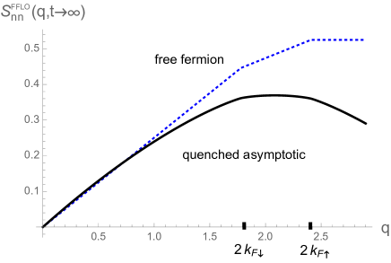
Figure 27: Asymptotic long-time limit of the number density structure function $S^{\mbox{\tiny FFLO}}_{nn}(q,t\to\infty)$ following the quantum quench $U\to 0$ at $t=0$ from the FFLO ground state for $K_{\rho}=1.6$ at $t=0^{-}$, as compared to the free fermion result.

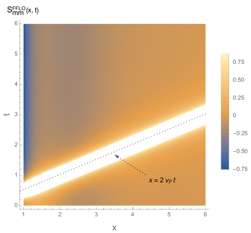
Figure 28: Space-time intensity plot of magnetization-magnetization correlation function $S^{\mbox{\tiny FFLO}}_{mm}(x,t)$ following a $U\to 0$ quench at $t=0$ from the FFLO state for $K_{\rho}=1.6$ at $t=0^{-}$. The light-cone boundary ($x=2v_{F}t$, the dotted line is a guide to the eye) separates early-time ground-state correlation from those in the asymptotic large time stationary state.

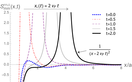
Figure 29: Magnetization-magnetization correlation function $S^{\mbox{\tiny FFLO}}_{mm}(x,t)$ following a $U\to 0$ quench at $t=0$ from the FFLO state for a series of times. The divergence peak moves as a wave-front at the light-cone $x_{*}(t)=2v_{F}t$.

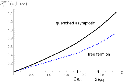
Figure 30: Asymptotic long-time limit of the magnetization structure function $S^{\mbox{\tiny FFLO}}_{mm}(q,t\to\infty)$ following the quantum quench $U\to 0$ at $t=0$ from the FFLO ground state for $K_{\rho}=1.6$ at $t=0^{-}$, as compared to the free fermion result.

The magnetization-magnetization correlation function is another important observable for identification of the FFLO ground state. Following a quench, it is given by

$$\begin{split}S^{\mbox{\tiny FFLO}}_{mm}(x)&\sim-\frac{1}{4}\left[\frac{2(\kappa/2+2/\kappa)a^{2}}{x^{2}}+\frac{(\kappa/2-2/\kappa)a^{2}}{(x+2v_{F}t)^{2}}+\frac{(\kappa/2-2/\kappa)a^{2}}{(x-2v_{F}t)^{2}}\right]\\ &\quad-\frac{\cos(2k_{F\uparrow}x)+\cos(2k_{F\downarrow}x)}{2}\left(\frac{a}{x}\right)^{(K_{\rho 0}+K^{-1}_{\rho 0}+\frac{\kappa}{2}+\frac{2}{\kappa})/2}\left|\frac{x^{2}-(2v_{F}t)^{2}}{(2v_{F}t)^{2}+a^{2}}\right|^{(\frac{2}{\kappa}-K_{\rho 0}+K^{-1}_{\rho 0}-\frac{\kappa}{2})/4},\\ &\sim\begin{cases}-\frac{\kappa}{2}\left(\frac{a}{x}\right)^{2}-\left(\frac{a}{x}\right)^{K_{\rho 0}+\kappa/2}\left(\frac{a}{2v_{F}t}\right)^{(\frac{2}{\kappa}-K_{\rho 0}+K^{-1}_{\rho 0}-\frac{\kappa}{2})/2}\frac{1}{2}\left[\cos(2k_{F\uparrow}x)+\cos(2k_{F\downarrow}x)\right],&x\gg 2v_{F}t,\\ \frac{1}{4}(\frac{2}{\kappa}-\frac{\kappa}{2})\frac{a^{2}}{(x-2v_{F}t)^{2}},&x\approx 2v_{\sigma}t,\\ -\frac{1}{2}(\frac{\kappa}{2}+\frac{2}{\kappa})\left(\frac{a}{x}\right)^{2}-\left(\frac{a}{x}\right)^{(K_{\rho 0}+K^{-1}_{\rho 0}+\frac{\kappa}{2}+\frac{2}{\kappa})/2}\frac{1}{2}\left[\cos(2k_{F\uparrow}x)+\cos(2k_{F\downarrow}x)\right],&x\ll 2v_{F}t,\end{cases}\end{split}$$ (109)

and is illustrated in Figs. 28 and 29. It displays a form quite similar to the density-density correlator $S^{\mbox{\tiny FFLO}}_{nn}(x,t)$.

Its long time limit in momentum space, $S^{\mbox{\tiny FFLO}}_{mm}(q,t\to\infty)$, is also illustrated in Fig. 30, showing that the $k_{F\uparrow,\downarrow}$ peaks are smoothed over in the long time limit.

X Summary and Conclusion

We used bosonization and the exact Luther-Emery mapping methods to study the dynamics of the 1D spin-imbalanced attractive Fermi-Hubbard model following a quench of its on-site interaction, $U\to 0$, particularly focusing on the long-time asymptotic behavior. We characterized the dynamics by evaluating a number of physically accessible post-quench correlation functions, such as the spin-singlet and triplet as well as the number and magnetization density correlators. On the scale of light-cone time $x/(2v_{F})$, these show a dephasing-driven evolution to a stationary state that exhibits strong qualitative dependence on the state of the initial pre-quench ground state.

The quench from the spin-gapped BCS ground state leads to a stationary state with a short-range correlated spin component (see Sec. IX.1), characterized by a correlation length $2\xi=2\pi v_{\sigma}/U$ for $x<x_{*}(t)=2v_{F}t$ and stationary power-law correlated charge component. The spin component matches the exponentially decaying spatial correlations of a noninteracting Fermi gas at finite temperature with correlation length $\xi_{T}=v_{F}/(2\pi T)$. This suggests that for quenches from the BCS state the spin-component thermalizes to the effective temperature,

$$T_{eff}=v_{F}/(4\pi\xi)\sim U,$$ (110)

while the gapless charge sector within the harmonic Luttinger liquid analysis remains pre-thermalized Yin1 ; Yin2 , i.e., does not thermalize. Thus we note that the extent to which the system appears to thermalize can depend on the measured observable, the level to which the gapped and gapless contributions contribute to its long-time behavior. For example, since the number density-density correlator [Eq. (103)] is dominated by the gapless charge sector, it shows no sign of thermalization (asymptotes to a power-law correlated pre-thermalized form) for a quench from the BCS ground state. On the other hand, the magnetization-magnetization correlator (105) is dominated by the gapped spin sector and appears to thermalize.

Furthermore, a quench from a ground state in the spin- (and charge-) gapless FFLO phase leads to a power-law stationary state for both spin and charge, thus neither thermalizes.

The thermalization and lack of it for the quench from gapped and gapless states, respectively, are consistent with the arguments in Refs. Cardy ; CardyJPhys ; Cardy2 , that a “deep” quench (defined by large ratio of initial to final gap, $\Delta_{0}/\Delta_{1}\gg 1$), e.g., a gapped to gapless Hamiltonian is necessary for thermalization, a conclusion based on results obtained using the generic method of slab construction, conformal field theory, and physical arguments. As emphasized by Cardy et al. Cardy2 , strictly speaking the state itself is neither stationary nor thermal. It is the local observables, expressible in terms of two-point correlation functions that thermalize in the thermodynamic limit by dephasing of an infinite number of momentum modes. For a local observable the relevant system is effectively open with the modes outside of the local region set by $x_{*}(t)$ acting like an effective bath.

Appendix A Green’s functions for Luther-Emery approach

In this section, we fill the technical gap leading to the ${\hat{\theta}}_{\sigma}$ correlation for Luther-Emery approach. Using Eq. (28) and Wick’s theorem, we obtain

$$\begin{split}\langle e^{i\sqrt{2}[{\hat{\theta}}_{\sigma}(x)-{\hat{\theta}}_{\sigma}(0)]}\rangle&=\langle e^{i2[{\hat{\theta}}(x)-{\hat{\theta}}(0)]}\rangle,\\ &=(2\pi a)^{2}\langle\hat{c}^{\dagger}_{R}(x)\hat{c}^{\dagger}_{L}(x)\hat{c}_{L}(0)\hat{c}_{R}(0)\rangle,\\ &\sim(2\pi a)^{2}[-G_{12}(x)G_{21}(x)+G_{11}(x)G_{22}(x)].\end{split}$$ (111)

Here the minus sign comes from the fermionic anti-commutation relation and the Green’s functions of ($\hat{c}_{R},\hat{c}_{L}$) are

$$G_{11}(x) =\sum_{p}\frac{e^{ipx}}{L}\langle\hat{c}^{\dagger}_{R}(p)\hat{c}_{R}(p)\rangle,$$ (112a)

$$G_{22}(x) =\sum_{p}\frac{e^{ipx}}{L}\langle\hat{c}^{\dagger}_{L}(p)\hat{c}_{L}(p)\rangle,$$ (112b)

$$G_{12}(x) =\sum_{p}\frac{e^{ipx}}{L}\langle\hat{c}^{\dagger}_{R}(p)\hat{c}_{L}(p)\rangle,$$ (112c)

$$G_{21}(x) =\sum_{p}\frac{e^{ipx}}{L}\langle\hat{c}^{\dagger}_{L}(p)\hat{c}_{R}(p)\rangle,$$ (112d)

which we will examine shortly how they behave asymptotically for the BCS state and the FFLO state, respectively. But before that, we notice the following to be true:

$$\begin{split}\langle e^{i\sqrt{2}[{\hat{\theta}}_{\sigma}(x)+{\hat{\theta}}_{\sigma}(0)]}\rangle&=(2\pi a)^{2}\langle\hat{c}^{\dagger}_{R}(x)\hat{c}^{\dagger}_{L}(x)\hat{c}^{\dagger}_{L}(0)\hat{c}^{\dagger}_{R}(0)\rangle=0,\end{split}$$ (113)

and therefore

$$\begin{split}\langle\cos(\sqrt{2}({\hat{\phi}}_{\sigma}(x))\cos(\sqrt{2}{\hat{\phi}}_{\sigma}(0))\rangle&=\frac{1}{2}\Re\left[\langle e^{i\sqrt{2}[{\hat{\theta}}_{\sigma}(x)-{\hat{\theta}}_{\sigma}(0)]}\rangle+\langle e^{i\sqrt{2}[{\hat{\theta}}_{\sigma}(x)+{\hat{\theta}}_{\sigma}(0)]}\rangle\right],\\ &=\frac{1}{2}\Re\langle e^{i\sqrt{2}[{\hat{\theta}}_{\sigma}(x)+{\hat{\theta}}_{\sigma}(0)]}\rangle.\end{split}$$ (114)

Here $\Re$ standards for the real-part.

The ${\hat{\phi}}_{\sigma}$ correlation turns out to be out of the reach of the LE approach. Unlike ${\hat{\theta}}_{\sigma}$, the ${\hat{\phi}}_{\sigma}$ correlation $\langle e^{i\sqrt{2}[{\hat{\phi}}_{\sigma}(x)-{\hat{\phi}}_{\sigma}(0)]}\rangle=\langle e^{i[{\hat{\phi}}(x)-{\hat{\phi}}(0)]}\rangle$ can not be related to the correlation of the spinless fermions ($\hat{c}_{R},\hat{c}_{L}$) in a simple way. Especially, we have

$$\begin{split}\langle\hat{c}^{\dagger}_{R}(x)\hat{c}_{L}(x)\hat{c}^{\dagger}_{L}(0)\hat{c}_{R}(0)\rangle&=(2\pi a)^{2}\langle e^{i2[{\hat{\phi}}(x)-{\hat{\phi}}(0)]}\rangle,\end{split}$$ (115)

and is not connected to $\langle e^{i[{\hat{\phi}}(x)-{\hat{\phi}}(0)]}\rangle$ since relation (25) no longer applies for the non-quadratic Hamiltonian (11).

A.1 Equilibrium BCS state

For the BCS state, the distribution of ($\hat{c}_{R},\hat{c}_{L}$) obeys Eq. (35), by using which we easily obtain

$$G_{12}(x) =-\int^{\infty}_{-\infty}\frac{dp}{2\pi}\frac{1}{2}\sin 2\beta_{p}=\frac{1}{\xi}\int^{\infty}_{0}\frac{dp}{2\pi}\frac{\cos(px/\xi)}{\sqrt{1+p^{2}}}=\frac{K_{0}(|\frac{x}{\xi}|)}{2\pi\xi},$$ (116a)

$$G_{11}(x) =\int^{\infty}_{-\infty}\frac{dp}{2\pi}\frac{1-\cos 2\beta_{p}}{2}e^{ipx}=-\frac{i}{\xi}\int^{\infty}_{0}\frac{dp}{2\pi}\frac{p\sin(px/\xi)}{\sqrt{1+p^{2}}}=i\frac{\partial_{x}K_{0}(x/\xi)}{2\pi\xi}=\frac{-iK_{1}(|\frac{x}{\xi}|)}{2\pi\xi},$$ (116b)

$$G_{22}(x) =\int^{\infty}_{-\infty}\frac{dp}{2\pi}\frac{1+\cos 2\beta_{p}}{2}e^{ipx}=-G_{11}(x)=i\frac{K_{1}(|\frac{x}{\xi}|)}{2\pi\xi},$$ (116c)

with $\tan 2\beta_{p}=-U/(\pi v_{\sigma}p)$. Here $\xi=\pi v_{\sigma}/U$ is the correlation length and $K_{0,1}$ are the modified Bessel functions satisfying

$$\begin{split}K_{z}(x)\to\sqrt{\frac{\pi}{2x}}e^{-x}(1+\frac{4z^{2}-1}{8x}+O(\frac{1}{x^{2}})),\;\;\;x>1.\end{split}$$ (117)

Plugging Eq. (116) inside (111), we then find for the gapped BCS state,

$$\begin{split}\langle e^{i\sqrt{2}[{\hat{\theta}}_{\sigma}(x)-{\hat{\theta}}_{\sigma}(0)]}\rangle&\sim\frac{a^{2}}{x^{2}}e^{-2x/\xi},\end{split}$$ (118)

which is Eq. (36) in the main text.

The corresponding average magnetization and the long-wavelength part of the magnetization-magnetization correlation function can also be evaluated as

$$\begin{split}\bar{m}&\equiv-\frac{1}{L}\int dx\frac{\sqrt{2}}{\pi}\langle\partial_{x}{\hat{\phi}}_{\sigma}(x)\rangle=\frac{\sqrt{2}}{L}\int dx\langle\hat{c}^{\dagger}_{R}\hat{c}_{R}+\hat{c}^{\dagger}_{L}\hat{c}_{L}\rangle=\frac{\sqrt{2}}{2\pi}\int^{\infty}_{-\infty}dp\langle\hat{c}^{\dagger}_{u}(p)c_{u}(p)\rangle\sim 0,\end{split}$$ (119)

and

$$\begin{split}\langle\partial_{x}{\hat{\phi}}_{\sigma}(x)\partial_{x^{\prime}}{\hat{\phi}}_{\sigma}(0)\rangle&=\sum_{n,n^{\prime}=R,L}\langle\hat{c}^{\dagger}_{n}(x)\hat{c}_{n}(x)\hat{c}^{\dagger}_{n^{\prime}}(0)\hat{c}_{n^{\prime}}(0)\rangle\sim\sum_{n,n^{\prime}=1,2}G_{nn^{\prime}}(x)G_{nn^{\prime}}(-x),\\ &\sim-\frac{1}{2\pi\xi x}e^{-2x/\xi}.\end{split}$$ (120)

A.2 Equilibrium FFLO state

For the FFLO state, the distribution of ($\hat{c}_{R},\hat{c}_{L}$) instead obeys Eq. (39) and the Green’s function $G_{11}(x)$ now becomes

$$\begin{split}G_{11}(x)&=\int^{\tilde{k}_{F}}_{-\tilde{k}_{F}}\frac{dp}{2\pi}e^{ipx}+\int^{\infty}_{\tilde{k}_{F}}\frac{dp}{2\pi}\frac{1-\cos 2\beta_{p}}{2}e^{ipx}+\int^{-\tilde{k}_{F}}_{-\infty}\frac{dp}{2\pi}\frac{1-\cos 2\beta_{p}}{2}e^{ipx},\\ &=\frac{1}{2}\int^{\tilde{k}_{F}}_{-\tilde{k}_{F}}\frac{dp}{2\pi}e^{ipx}-\frac{i}{\xi}\int^{\infty}_{\tilde{k}_{F}\xi}\frac{dp}{2\pi}\frac{p\sin(px/\xi)}{\sqrt{1+p^{2}}},\\ &=-\frac{K_{1}(x/\xi)}{2\pi\xi}+\frac{i}{\xi}\int^{\tilde{k}_{F}\xi}_{0}\frac{dp}{2\pi}\frac{p\sin(px/\xi)}{\sqrt{1+p^{2}}}+\frac{\sin(\tilde{k}_{F}x)}{2\pi x}.\end{split}$$ (121)

Focusing on long-distance asymptotic behavior, we can throw away the $K_{1}(x)$ part that decays exponentially. We can further simplify the second term in the above equation by noticing $\tilde{k}_{F}\xi<1$ generically true for small spin imbalance (which is the case we consider throughout the paper), and thereby obtain

$$\begin{split}G_{11}(x)&\sim\frac{i}{\xi}\int^{\tilde{k}_{F}\xi}_{0}\frac{dp}{2\pi}p\sin(px/\xi)+\frac{\sin(\tilde{k}_{F}x)}{2\pi x},\\ &\sim\frac{\sin(\tilde{k}_{F}x)-i\tilde{k}_{F}\xi\cos(\tilde{k}_{F}x)}{2\pi x}+\frac{i\xi\sin(\tilde{k}_{F}x)}{2\pi x^{2}}.\end{split}$$ (122)

The other Green’s functions can be obtained in a similar way as

$$\begin{split}G_{22}(x)&\sim\frac{\sin(\tilde{k}_{F}x)+i\tilde{k}_{F}\xi\cos(\tilde{k}_{F}x)}{2\pi x}-\frac{i\xi\sin(\tilde{k}_{F}x)}{2\pi x^{2}},\end{split}$$ (123)

and

$$\begin{split}G_{12}(x)=G_{21}(x)&\sim-\frac{\sin(\tilde{k}_{F}x)(1-(\tilde{k}_{F}\xi)^{2}/2)}{2\pi x}+\frac{\cos(\tilde{k}_{F}x)\tilde{k}_{F}\xi^{2}_{0}}{2\pi x^{2}}.\end{split}$$ (124)

Plugging them back into Eq. (111), we then obtain the ${\hat{\theta}}_{\sigma}$ correlation for the spin-gapless FFLO state to lowest order as

$$\begin{split}\langle e^{i\sqrt{2}[{\hat{\theta}}_{\sigma}(x)-{\hat{\theta}}_{\sigma}(0)]}\rangle&\sim\frac{a^{2}}{x^{2}}[-\sin^{2}(\tilde{k}_{F}x)(1-(\tilde{k}_{F}\xi)^{2}/2)^{2}+\sin^{2}(\tilde{k}_{F}x)+(\tilde{k}_{F}\xi)^{2}\cos^{2}(\tilde{k}_{F}x)],\\ &\sim(\tilde{k}_{F}\xi)^{2}\frac{a^{2}}{x^{2}},\end{split}$$ (125)

which is Eq. (41) in the main text.

Similarly, the average magnetization and its correlation function’s long-wavelength part are evaluated as

$$\begin{split}\bar{m}&=\frac{\sqrt{2}}{2\pi}\int^{\infty}_{-\infty}dp\langle\hat{c}^{\dagger}_{u}(p)c_{u}(p)\rangle=\frac{\sqrt{2}\tilde{k}_{F}}{\pi}\sim\frac{\sqrt{2}\sqrt{h^{2}-U^{2}/(\pi a)^{2}}}{\pi v_{\sigma}},\end{split}$$ (126)

and

$$\begin{split}\langle\partial_{x}{\hat{\phi}}_{\sigma}(x)\partial_{x^{\prime}}{\hat{\phi}}_{\sigma}(0)\rangle\sim\sum_{n,n^{\prime}=1,2}G_{nn^{\prime}}(x)G_{nn^{\prime}}(-x)\sim-\frac{\sin^{2}(\tilde{k}_{F}x)}{\pi^{2}x^{2}}.\end{split}$$ (127)

Appendix B Semi-classical approach for equilibrium BCS state

In this section, we derive the ${\hat{\phi}}_{\sigma}$ correlation [Eq. (48)] for equilibrium BCS state within the semiclassical approach in details. Using relation,

$${\hat{\phi}}_{\sigma}(x)=-\sqrt{K_{\sigma}}\frac{i\pi}{L}\sum_{p\neq 0}\left(\frac{L|p|}{2\pi}\right)^{1/2}\frac{1}{p}e^{-a|p|/2-ipx}(\hat{b}^{\dagger}_{p}+\hat{b}_{-p}),$$ (128a)

$${\hat{\theta}}_{\sigma}(x)=\frac{1}{\sqrt{K_{\sigma}}}\frac{i\pi}{L}\sum_{p\neq 0}\left(\frac{L|p|}{2\pi}\right)^{1/2}\frac{1}{|p|}e^{-a|p|/2-ipx}(\hat{b}^{\dagger}_{p}-\hat{b}_{-p}),$$ (128b)

and the statistics of ($\hat{b}_{p},\hat{b}_{p}^{\dagger}$) Eq. (47), we have

$$\begin{split}\langle({\hat{\phi}}_{\sigma}(x)-{\hat{\phi}}_{\sigma}(0))^{2}\rangle&=K_{\sigma}\int^{\infty}_{0}\frac{dp}{p}e^{-ap}[1-\cos(px)]\left[\langle\hat{b}^{\dagger}_{p}\hat{b}^{\dagger}_{-p}\rangle+\langle\hat{b}^{\dagger}_{p}\hat{b}_{p}\rangle+\langle\hat{b}_{-p}\hat{b}^{\dagger}_{-p}\rangle+\langle\hat{b}_{p}\hat{b}_{-p}\rangle\right],\\ &=K_{\sigma}\int^{\infty}_{0}\frac{dp}{\sqrt{p^{2}+1/\lambda^{2}}}e^{-ap}[1-\cos(px)],\\ &=K_{\sigma}[\operatorname{ArcSinh}(\lambda/a)-K_{0}(x/\lambda)],\\ &\sim\operatorname{const},\end{split}$$ (129)

where $\operatorname{const}=K_{\sigma}\operatorname{ArcSinh}(\lambda/a)\sim O(1)$ and for long distance behavior we have ignored $K_{0}(x)$ that decays exponentially.

The ${\hat{\theta}}_{\sigma}$ correlation can be evaluated in a similar way. We have

$$\begin{split}\langle({\hat{\theta}}_{\sigma}(x)-{\hat{\theta}}_{\sigma}(0))^{2}\rangle&=\frac{1}{K_{\sigma}}\int^{\infty}_{0}\frac{dp}{p}e^{-ap}[1-\cos(px)]\left[\langle\hat{b}_{-p}\hat{b}^{\dagger}_{-p}\rangle+\langle\hat{b}^{\dagger}_{p}\hat{b}_{p}\rangle-\langle\hat{b}^{\dagger}_{p}\hat{b}^{\dagger}_{-p}\rangle-\langle\hat{b}_{p}\hat{b}_{-p}\rangle\right],\\ &=\frac{1}{K_{\sigma}}\int^{\infty}_{0}\frac{dp\sqrt{p^{2}+1/\lambda^{2}}}{p^{2}}e^{-ap}[1-\cos(px)],\\ &=\frac{1}{K_{\sigma}}\int^{\infty}_{0}dp\left[\frac{1}{\sqrt{p^{2}+1/\lambda^{2}}}+\frac{1}{\lambda^{2}p^{2}\sqrt{p^{2}+1/\lambda^{2}}}\right]e^{-ap}[1-\cos(px)],\\ &=\frac{1}{K_{\sigma}}\left[\operatorname{ArcSinh}(\lambda/a)-K_{0}(x/\lambda)-1-\frac{1}{2}G^{21}_{13}\left(\frac{x^{2}}{4\lambda^{2}}\bigg{|}\begin{matrix}&3/2&\\ 0&1&1/2\end{matrix}\right)\right],\\ &\sim-x/\xi_{0}+\operatorname{const},\end{split}$$ (130)

with $\xi_{0}=2\lambda K_{\sigma}/\pi$ and $\operatorname{const}=[\operatorname{ArcSinh}(\lambda/a)-1]/K_{\sigma}\sim O(1)$. Here we have used the property of MeijerG function $G^{21}_{13}$

$$\begin{split}\frac{1}{2\lambda^{2}}\int^{\infty}_{0}dp\frac{1}{p^{2}\sqrt{p^{2}+1/\lambda^{2}}}e^{-ap}[1-\cos(px)]&=-\frac{1}{2}-\frac{1}{4}G^{21}_{13}\left(\frac{x^{2}}{4\lambda^{2}}\bigg{|}\begin{matrix}&3/2&\\ 0&1&1/2\end{matrix}\right),\\ &\sim\frac{\pi}{4}\frac{x}{\lambda}-\frac{1}{2},\;\;\;x>1.\end{split}$$ (131)

Appendix C Normal modes approach for charge sector dynamics

In this section, we fill in some technical details leading to the charge sector quench dynamics results [Eq. (LABEL:quenchluttingerphitheta) and (LABEL:quenchluttingerphitheta2)], obtained with the normal mode approach in the main text. Using Eq. (75), we have

$$\langle b^{\dagger}_{p}(t)b_{p}(t)\rangle =\langle b^{\dagger}_{-p}(t)b_{-p}(t)\rangle,$$

$$=\cosh^{2}\beta_{1}\sinh^{2}(\beta_{1}-\beta_{0})+\sinh^{2}\beta_{1}\cosh^{2}(\beta_{1}-\beta_{0})-\frac{1}{2}\sinh 2\beta_{1}\sinh 2(\beta_{1}-\beta_{0})\cos(2v_{\rho 1}pt),$$ (132a)

$$\langle b^{\dagger}_{p}(t)b^{\dagger}_{-p}(t)\rangle =\langle b_{p}(t)b_{-p}(t)\rangle,$$

$$=\frac{\cosh^{2}\beta_{1}}{2}\sinh 2(\beta_{1}-\beta_{0})e^{2iv_{\rho 1}|p|t}+\frac{\sinh^{2}\beta_{1}}{2}\sinh 2(\beta_{1}-\beta_{0})e^{-2iv_{\rho 1}|p|t}-\frac{1}{2}\sinh(2\beta_{1})\cosh 2(\beta_{1}-\beta_{0}),$$ (132b)

$$\langle b^{\dagger}_{p}(t)b^{\dagger}_{p}(t)\rangle =\langle b_{-p}(t)b_{-p}(t)\rangle=\langle b^{\dagger}_{p}(t)b_{-p}(t)\rangle=0.$$ (132c)

Summing them up, we obtain

$$\langle\hat{b}^{\dagger}_{p}\hat{b}^{\dagger}_{-p}\rangle+\langle\hat{b}^{\dagger}_{p}\hat{b}_{p}\rangle+\langle\hat{b}_{-p}\hat{b}^{\dagger}_{-p}\rangle+\langle b_{p}\hat{b}_{-p}\rangle =A_{1}+A_{2}\cos(2v_{\rho 1}pt),$$ (133a)

$$\langle b_{-p}b^{\dagger}_{-p}\rangle+\langle b^{\dagger}_{p}b_{p}\rangle-\langle b^{\dagger}_{p}b^{\dagger}_{-p}\rangle-\langle b_{p}b_{-p}\rangle =B_{1}+B_{2}\cos(2v_{\rho 1}pt),$$ (133b)

where

$$A_{1} =\frac{1}{2}[(\cosh\beta_{0}-\sinh\beta_{0})^{2}+(\cosh(2\beta_{1}-\beta_{0})-\sinh(2\beta_{1}-\beta_{0}))^{2}]=\frac{1}{2}(K_{\rho 0}+\frac{K^{2}_{\rho 1}}{K_{\rho 0}}),$$ (134a)

$$A_{2} =\frac{1}{2}[(\cosh\beta_{0}-\sinh\beta_{0})^{2}-(\cosh(2\beta_{1}-\beta_{0})-\sinh(2\beta_{1}-\beta_{0}))^{2}]=\frac{1}{2}(K_{\rho 0}-\frac{K^{2}_{\rho 1}}{K_{\rho 0}}),$$ (134b)

$$B_{1} =\frac{1}{2}[(\cosh\beta_{0}-\sinh\beta_{0})^{2}+(\cosh(2\beta_{1}-\beta_{0})-\sinh(2\beta_{1}-\beta_{0}))^{2}]=\frac{1}{2}(\frac{1}{K_{\rho 0}}+\frac{K_{\rho 0}}{K^{2}_{\rho 1}}),$$ (134c)

$$B_{2} =\frac{1}{2}[(\cosh\beta_{0}-\sinh\beta_{0})^{2}-(\cosh(2\beta_{1}-\beta_{0})-\sinh(2\beta_{1}-\beta_{0}))^{2}]=\frac{1}{2}(\frac{1}{K_{\rho 0}}-\frac{K_{\rho 0}}{K^{2}_{\rho 1}}).$$ (134d)

Thus the ${\hat{\theta}}_{\rho}$ and ${\hat{\phi}}_{\rho}$ correlations become

$$\begin{split}\langle[{\hat{\phi}}_{\rho}(x,t)-{\hat{\phi}}_{\rho}(0,t)]^{2}\rangle&=\int^{\infty}_{0}\frac{dp}{p}e^{-ap}[1-\cos(px)]\langle(\hat{b}^{\dagger}_{p}(t)+\hat{b}_{-p}(t))(\hat{b}^{\dagger}_{-p}(t)+\hat{b}_{p}(t))\rangle,\\ &=\int^{\infty}_{0}\frac{dp}{p}e^{-ap}[1-\cos(px)](A_{1}+A_{2}\cos(2v_{F}pt)),\\ &=A_{1}\ln\left[\frac{x}{a}\right]+\frac{1}{2}A_{2}\ln\left|\frac{x^{2}-(2v_{F}t)^{2}}{a^{2}+(2v_{F}t)^{2}}\right|,\end{split}$$ (135)

and

$$\begin{split}\langle[{\hat{\theta}}_{\rho}(x,t)-{\hat{\theta}}_{\rho}(0,t)]^{2}\rangle&=\int^{\infty}_{0}\frac{dp}{p}e^{-ap}[1-\cos(px)]\langle(\hat{b}^{\dagger}_{p}(t)-\hat{b}_{-p}(t))(\hat{b}^{\dagger}_{-p}(t)-\hat{b}_{p}(t))\rangle,\\ &=\int^{\infty}_{0}\frac{dp}{p}e^{-ap}[1-\cos(px)](B_{1}+B_{2}\cos(2v_{F}pt)),\\ &=B_{1}\ln\left[\frac{x}{a}\right]+\frac{1}{2}B_{2}\ln\left|\frac{x^{2}-(2v_{F}t)^{2}}{a^{2}+(2v_{F}t)^{2}}\right|,\end{split}$$ (136)

At $t=0$, above equations reduce to

$$\langle[{\hat{\phi}}(x,t)-{\hat{\phi}}(0,t)]^{2}\rangle =K_{\rho 0}\ln\left[\frac{x}{a}\right],$$ (137a)

$$\langle[{\hat{\theta}}(x,t)-{\hat{\theta}}(0,t)]^{2}\rangle =\frac{1}{K_{\rho 0}}\ln\left[\frac{x}{a}\right],$$ (137b)

consistent with the initial pre-quench results Eqs. (24b) and (23b), as expected. Using relation (25), we are easy to see they reproduce the results Eqs. (LABEL:quenchluttingerphitheta) and (LABEL:quenchluttingerphitheta2) in the main text.

Appendix D Normal modes approach for spin sector BCS quench dynamics

In the main text, we use the Heinsenberg equations of motion approach to study the quench dynamics for the spin sector. In this appendix, we list the normal modes approach for the spin sector dynamics, for completeness purpose as well as possible generalization to other quench protocols.

Substituting ${\hat{\phi}}_{\sigma}(x),{\hat{\theta}}_{\sigma}(x)$ using relation (128) into the post-quench Hamiltonian, we obtain the post-quench Hamiltonian in terms of bosonic creation and annihilation operator as

$$\begin{split}\hat{H}_{\sigma}&=\frac{1}{4}\sum_{p\neq 0}v_{F}|p|\Big{[}(1/K_{\sigma}+K_{\sigma})(\hat{b}^{\dagger}_{p}\hat{b}_{p}+\hat{b}^{\dagger}_{-p}\hat{b}_{-p})+(K_{\sigma}-1/K_{\sigma})(\hat{b}^{\dagger}_{p}\hat{b}^{\dagger}_{-p}+\hat{b}_{p}\hat{b}_{-p})\Big{]},\end{split}$$ (138)

which is not diagonal since the Luttinger parameter is also quenched as $K_{\sigma}\to 1$ following the interaction quench $U\to 0$. It can be diagonalized by the following Bogoliubov transformation:

$$\begin{split}\begin{pmatrix}\hat{b}_{p}\\ \hat{b}^{\dagger}_{-p}\end{pmatrix}=\begin{pmatrix}\cosh\beta&\sinh\beta\\ \sinh\beta&\cosh\beta\end{pmatrix}\begin{pmatrix}\hat{\chi}_{p}\\ \hat{\chi}^{\dagger}_{-p}\end{pmatrix}\equiv U_{\sigma}(0^{+})\begin{pmatrix}\hat{\chi}_{p}\\ \hat{\chi}^{\dagger}_{-p}\end{pmatrix}\end{split}$$ (139)

with $e^{-2\beta}=K_{\sigma}$.

Prior to the quench, we know from Eq. (44) that the initial Hamiltonian is diagonalized by

$$\begin{split}\begin{bmatrix}\hat{b}_{p}\\ \hat{b}^{\dagger}_{-p}\\ \end{bmatrix}=\begin{bmatrix}u_{p}&-v_{p}\\ -v_{p}&u_{p}\\ \end{bmatrix}\begin{bmatrix}\hat{\alpha}_{p}\\ \hat{\alpha}^{\dagger}_{-p}\\ \end{bmatrix}\equiv U_{\sigma}(0^{-})\begin{bmatrix}\hat{\alpha}_{p}\\ \hat{\alpha}^{\dagger}_{-p}\\ \end{bmatrix}.\end{split}$$ (140)

The dynamics is easily encoded in the form of ($\hat{\chi}_{p}(t),\hat{\chi}^{\dagger}_{p}(t)$), which satisfies

$$\begin{split}\begin{pmatrix}\hat{\chi}_{p}(t)\\ \hat{\chi}^{\dagger}_{-p}(t)\end{pmatrix}=\begin{pmatrix}e^{iv_{F}|p|t}&0\\ 0&e^{-iv_{F}|p|t}\end{pmatrix}\begin{pmatrix}\hat{\chi}_{p}\\ \hat{\chi}^{\dagger}_{-p}\end{pmatrix}\equiv U_{\sigma T}(t)\begin{pmatrix}\hat{\chi}_{p}\\ \hat{\chi}^{\dagger}_{-p}\end{pmatrix}.\end{split}$$ (141)

Thus following what is done in the charge sector dynamics section, we obtain similarly

$$\begin{split}\begin{bmatrix}\hat{b}_{p}(t)\\ \hat{b}^{\dagger}_{-p}(t)\\ \end{bmatrix}&=U_{\sigma}(0^{+})U_{\sigma T}(t)U_{\sigma}(0^{+})U_{\sigma}(0^{-})\begin{bmatrix}\hat{\alpha}_{p}\\ \hat{\alpha}^{\dagger}_{-p}\\ \end{bmatrix}.\end{split}$$ (142)

Combining it with Eqs. (128) and (45), we then find

$$\begin{split}&\quad\langle({\hat{\phi}}_{\sigma}(x,t)-{\hat{\phi}}_{\sigma}(0,t))^{2}\rangle\\ &=K_{\sigma}\int^{\infty}_{0}\frac{dp}{p}e^{-ap}[1-\cos(px)]\left[\langle\hat{b}^{\dagger}_{p}(t)\hat{b}^{\dagger}_{-p}(t)\rangle+\langle\hat{b}^{\dagger}_{p}(t)\hat{b}_{p}(t)\rangle+\langle\hat{b}_{-p}(t)\hat{b}^{\dagger}_{-p}(t)\rangle+\langle b_{p}(t)\hat{b}_{-p}(t)\rangle\right],\\ &=K_{\sigma}\int^{\infty}_{0}\frac{dp}{p}e^{-ap}[1-\cos(px)]\left[(1+2v^{2}_{p}-2u_{p}v_{p})[1+(K^{-2}_{\sigma}-1)(1-\cos(2v_{F}pt))/2]+2K^{-2}_{\sigma}u_{p}v_{p}[1-\cos(2v_{F}pt)]\right],\\ &=K_{\sigma}\int^{\infty}_{0}\frac{dp}{\sqrt{p^{2}+1/\lambda^{2}}}e^{-ap}[1-\cos(px)][1+(K^{-2}_{\sigma}-1)(1-\cos(2v_{F}pt))/2],\\ &\quad+\frac{1}{2K_{\sigma}\lambda^{2}}\int^{\infty}_{0}\frac{dp}{p^{2}\sqrt{p^{2}+1/\lambda^{2}}}e^{-ap}[1-\cos(px)][1-\cos(2v_{F}pt)],\\ &\sim\frac{K^{-1}_{\sigma}+K_{\sigma}}{2}\operatorname{ArcSinh}(\lambda/a)+Z(x,t),\end{split}$$ (143)

where

$$\begin{split}Z(x,t)&\equiv\frac{1}{2K_{\sigma}\lambda^{2}}\int^{\infty}_{0}\frac{dp}{p^{2}\sqrt{p^{2}+1/\lambda^{2}}}e^{-ap}[1-\cos(px)][1-\cos(2pv_{F}t)],\\ &=\frac{1}{2K_{\sigma}\lambda^{2}}\int^{\infty}_{0}\frac{dp}{p^{2}\sqrt{p^{2}+1/\lambda^{2}}}e^{-ap}\left(1-\cos(px)+1-\cos(2pv_{F}t)-\frac{1-\cos(p(x-2v_{F}t))}{2}-\frac{1-\cos(p(x+2v_{F}t))}{2}\right),\\ &\sim\frac{\pi}{8K_{\sigma}\lambda}\left(x+2v_{F}t-|x-2v_{F}t|\right)-\frac{1}{2K_{\sigma}},\\ &\sim\begin{cases}\frac{2v_{F}t}{2\xi}-\frac{1}{2K_{\sigma}},&x\gg 2v_{F}t,\\ \frac{x}{2\xi}-\frac{1}{2K_{\sigma}},&x\ll 2v_{F}t,\end{cases}\end{split}$$ (144)

and we have used the Meijer G function property (131) once again. The ${\hat{\phi}_{\sigma}}$ correlation can then be evaluated as

$$\begin{split}\langle e^{i\sqrt{2}[{\hat{\phi}}_{\sigma}(x,t)-{\hat{\phi}}_{\sigma}(0,t)]}\rangle&\sim e^{-Z(x,t)}\sim\begin{cases}e^{-\frac{2v_{F}t}{2\xi}},&x\gg 2v_{F}t,\\ e^{-\frac{x}{2\xi}},&x\ll 2v_{F}t,\end{cases}\end{split}$$ (145)

which is Eq. (94) in the main text.

Similarly, for the ${\hat{\theta}}_{\sigma}-{\hat{\theta}}_{\sigma}$ correlation we have

$$\begin{split}&\quad\langle({\hat{\theta}}_{\sigma}(x,t)-{\hat{\theta}}_{\sigma}(0,t))^{2}\rangle\\ &=\frac{1}{K_{\sigma}}\int^{\infty}_{0}\frac{dp}{p}e^{-ap}[1-\cos(px)]\left[\langle\hat{b}^{\dagger}_{p}(t)\hat{b}_{p}(t)\rangle+\langle\hat{b}_{-p}(t)\hat{b}^{\dagger}_{-p}(t)\rangle-\langle\hat{b}^{\dagger}_{p}(t)\hat{b}^{\dagger}_{-p}(t)\rangle-\langle b_{p}(t)\hat{b}_{-p}(t)\rangle\right],\\ &=\frac{1}{K_{\sigma}}\int^{\infty}_{0}\frac{dp}{p}e^{-ap}[1-\cos(px)]\left[(1+2v^{2}_{p}-2u_{p}v_{p})[1+(K^{2}_{\sigma}-1)(1-\cos(2v_{F}pt))/2]+2u_{p}v_{p}[1+\cos(2v_{F}pt)]\right],\\ &=\frac{1}{K_{\sigma}}\int^{\infty}_{0}dp\frac{\sqrt{p^{2}+1/\lambda^{2}}}{p^{2}}e^{-ap}[1-\cos(px)][1+(K^{2}_{\sigma}-1)(1-\cos(2v_{F}pt))/2],\\ &\quad+\frac{1}{2K_{\sigma}\lambda^{2}}\int^{\infty}_{0}\frac{dp}{p^{2}\sqrt{p^{2}+1/\lambda^{2}}}e^{-ap}[1-\cos(px)][1+\cos(2v_{F}pt)],\\ &\sim\frac{K^{-1}_{\sigma}+K_{\sigma}}{2}\operatorname{ArcSinh}(\lambda/a)+Z^{\prime}(x,t),\end{split}$$ (146)

where

$$\begin{split}Z^{\prime}(x,t)&\equiv\frac{1}{2K_{\sigma}\lambda^{2}}\int^{\infty}_{0}\frac{dp}{p^{2}\sqrt{p^{2}+1/\lambda^{2}}}e^{-ap}[1-\cos(px)][1+\cos(2pv_{F}t)],\\ &=\frac{1}{2K_{\sigma}\lambda^{2}}\int^{\infty}_{0}\frac{dp}{p^{2}\sqrt{p^{2}+1/\lambda^{2}}}e^{-ap}\left(1-\cos(px)-(1-\cos(2pv_{F}t))+\frac{(1-\cos(p(x-2v_{F}t))}{2}+\frac{(1-\cos(p(x+2v_{F}t))}{2}\right),\\ &\sim\frac{\pi}{8K_{\sigma}\lambda}(3x-2v_{F}t+|x-2v_{F}t|)-\frac{1}{2K_{\sigma}},\\ &\sim\begin{cases}\frac{x-v_{F}t}{\xi_{0}}-\frac{1}{2K_{\sigma}},&x\gg 2v_{F}t,\\ \frac{x}{2\xi_{0}}-\frac{1}{2K_{\sigma}},&x\ll 2v_{F}t.\end{cases}\end{split}$$ (147)

The ${\hat{\theta}}_{\sigma}$ correlation thereby is

$$\begin{split}\langle e^{i\sqrt{2}[{\hat{\theta}}_{\sigma}(x)-{\hat{\theta}}_{\sigma}(0)]}\rangle&\propto e^{-Z^{\prime}(x,t)}\sim\begin{cases}e^{-\frac{x-2v_{F}t}{\xi_{0}}},&x\gg 2v_{F}t,\\ e^{-\frac{x}{2\xi_{0}}},&x\ll 2v_{F}t.\end{cases}\end{split}$$ (148)

which we recognize as Eq. (95) in the main text. It is also worth noting that the following correlations

$$\langle e^{i\sqrt{2}[{\hat{\phi}}_{\sigma}(x,t)+{\hat{\phi}}_{\sigma}(0,t)]}\rangle =0,$$ (149a)

$$\langle e^{i\sqrt{2}[{\hat{\theta}}_{\sigma}(x,t)+{\hat{\theta}}_{\sigma}(0,t)]}\rangle =0,$$ (149b)

are both zero.

Generalizing the above apporoach to other quench protocols such as $U\to U^{\prime}\neq 0$ should also be straightforward. In that case, the Hamiltonian (138) will contain extra terms from the finite nonlinearity $U^{\prime}\cos{\hat{\phi}}_{\sigma}$ term, which can be again expressed in terms of quadratic operators of ($\hat{b}_{p},\hat{b}^{\dagger}_{p}$) by expanding the cosine potential around its minimum. The post-quench dynamics will be governed by a matrix similar to Eq. (141), but with $v_{F}$ being replaced with the post-quench spin velocity $v_{\sigma 1}$. Other than that, the calculation procedure follows exactly the same as the one discussed above. We leave this generalization to future work.

Appendix E Wick’s theorem for Multiple fields

For Gaussian field $\tilde{\phi}(x)$, the relation (25) can be generalized to the multiple fields case as

$$\begin{split}\langle e^{i\sum_{j}n_{j}{\hat{\phi}}(x_{j})}\rangle&=e^{-\frac{1}{2}\langle\left(\sum_{i}n_{i}{\hat{\phi}}(x_{i})\right)^{2}\rangle}\\ &=e^{-\frac{1}{2}\sum_{i}n^{2}_{i}\langle{\hat{\phi}}^{2}(0)\rangle-\sum_{i>j}n_{i}n_{j}\langle\hat{\phi}(x_{i})\hat{\phi}(x_{j})\rangle}\\ &=e^{-\frac{1}{2}\left(\sum_{i}n_{i}\right)^{2}\langle{\hat{\phi}}^{2}(0)\rangle+\frac{1}{2}\sum_{i>j}n_{i}n_{j}\langle(\hat{\phi}(x_{i})-\hat{\phi}(x_{j}))^{2}\rangle}\\ &=e^{-\frac{1}{2}\left(\sum_{i}n_{i}\right)^{2}\ln(L/a)+\frac{1}{2}\sum_{i>j}n_{i}n_{j}\langle(\hat{\phi}(x_{i})-\hat{\phi}(x_{j}))^{2}\rangle}\\ &=\delta\left(\sum_{i}n_{i}\right)e^{\frac{1}{2}\sum_{i>j}n_{i}n_{j}\langle(\hat{\phi}(x_{i})-\hat{\phi}(x_{j}))^{2}\rangle]},\end{split}$$ (150)

where $\delta$ is the Kronicker delta function.

References

- (1) I. Bloch, J. Dalibard, and W. Zwerger, Rev. Mod. Phys. 80, 885 (2008).
- (2) W. Ketterle and M. Zwierlein, in Ultracold Fermi Gases, Proceedings of the International School of Physics ”Enrico Fermi”, Course CLXIV, Varenna, 2006, edited by M. Inguscio, W. Ketterle, and C. Salomon (IOS Press, Amsterdam, 2008), pp. 95-287.
- (3) V. Gurarie and L. Radzihovsky, Ann. Phys. 322, 2 (2007).
- (4) D. E. Sheehy and L. Radzihovsky, Ann. Phys. 322, 1790 (2007).
- (5) S. Giorgini, L. P. Pitaevskii, and S. Stringari, Rev. Mod. Phys. 80, 1215 (2008).
- (6) L. Radzihovsky and D. E. Sheehy, Rep. Prog. Phys. 73, 076501 (2010).
- (7) C. Regal, M. Greiner and D. S. Jin, Phys. Rev. Lett. 92, 040403 (2004). .
- (8) M. W. Zwierlein, C. A. Stan, C. H. Schunck, S. M. F. Raupach, A. J. Kerman, and W. Ketterle, Phys. Rev. Lett. 92, 120403 (2004)
- (9) J. Kinast, S. L. Hemmer, M. E. Gehm, A. Turlapov, and J. E. Thomas, Phys. Rev. Lett. 92, 150402 (2004)
- (10) M. Bartenstein, A. Altmeyer, S. Riedl, S. Jochim, C. Chin, J. H. Denschlag, and R. Grimm, Phys. Rev. Lett. 92, 120401 (2004).
- (11) T. Bourdel, L. Khaykovich, J. Cubizolles, J. Zhang, F. Chevy, M. Teichmann, L. Tarruell, S. J. J. M. F. Kokkelmans, and C. Salomon, Phys. Rev. Lett. 93, 050401 (2004).
- (12) D. M. Eagles, Phys. Rev. 186, 456 (1969).
- (13) A. J. Leggett, in Modern Trends in the Theory of Condensed Matter, edited by A. Pekalski and R. Przystawa (Springer-Verlag, Berlin, 1980), pp. 13-27
- (14) P. Nozieres and S. Schmitt-Rink, J. Low Temp. Phys. 59, 195 (1985).
- (15) C. A. R. Sade Melo, M. Randeria, and J. R. Engelbrecht, Phys. Rev. Lett. 71, 3202 (1993).
- (16) E. Timmermans, K. Furuya, P. W. Milonni, and A. K. Kerman, Phys. Lett. A 285, 228 (2001).
- (17) M. Holland, S. J. J. M. F. Kokkelmans, M. L. Chiofalo, and R. Walser, Phys. Rev. Lett. 87, 120406 (2001).
- (18) Y. Ohashi and A. Griffin, Phys. Rev. Lett. 89, 130402 (2002); Phys. Rev. A 67, 033603 (2003).
- (19) A. V. Andreev, V. Gurarie, and L. Radzihovsky, Phys. Rev. Lett. 93, 130402 (2004).
- (20) J. Stajic, J. N. Milstein, Q. Chen, M. L. Chiofalo, M. J. Holland, and K. Levin, Phys. Rev. A 69, 063610 (2004).
- (21) G. B. Partridge, G. B., K. E. Strecker, R. I. Kamar, M. W. Jack, and R. G. Hulet, Phys. Rev. Lett. 95, 020404 (2005)
- (22) C. Chin, M. Bartenstein, A. Altmeyer, S. Riedl, S. Jochim, J. Hecker Denschlag, and R. Grimm, Science 305, 5687 (2004).
- (23) M. W. Zwierlein, A. Schirotzek, C. H. Schunck, and W. Ketterle, Science 311, 492 (2006).
- (24) G. B. Partridge, W. Li, R. I. Kamar, Y. Liao, and R. G. Hulet, Science 311, 5760 (2006).
- (25) Y. Shin, M. W. Zwierlein, C. H. Schunck, A. Schirotzek, and W. Ketterle, Phys. Rev. Lett. 97, 030401 (2006).
- (26) S. Nascimbene, N. Navon, K. J. Jiang, L. Tarruell, M. Teichmann, J. Mckeever, F. Chevy, and C. Salomon, Phys. Rev. Lett. 103, 170402 (2009).
- (27) R. Combescot, EPL 55, 150 (2001).
- (28) W. V. Liu and F. Wilczek, Phys. Rev. Lett. 90, 047002 (2003).
- (29) P. F. Bedaque, H. Caldas, and G. Rupak, Phys. Rev. Lett. 91, 247002 (2003).
- (30) H. Caldas, Phys. Rev. A 69, 063602 (2004).
- (31) J. Carlson and S. Reddy, Phys. Rev. Lett. 95, 060401 (2005).
- (32) T. D. Cohen, Thomas D, Phys. Rev. Lett. 95, 120403 (2005).
- (33) D. E. Sheehy and L. Radzihovsky, Phys. Rev. Lett. 96, 060401 (2006).
- (34) C-H. Pao, S-T. Wu, and S-K. Yip, Phys. Rev. B 73, 132506 (2006).
- (35) D. T. Son and M. A. Stephanov, Phys. Rev. A 74, 013614 (2006).
- (36) D. E. Sheehy and L. Radzihovsky, Phys. Rev. B 75, 136501 (2007).
- (37) P. Castorina, M. Grasso, M. Oertel, M. Urban, and D. Zappala, Phys. Rev. A 72, 025601 (2005).
- (38) A. Sedrakian, J. Mur-Petit, A. Polls, and H Muther, Phys. Rev. A 72, 013613 (2005).
- (39) A. Bulgac, M. M. Forbes, and A. Schwenk, Phys. Rev. Lett. 97, 020402 (2006).
- (40) J. Dukelsky, G. Ortiz, S. M. A. Rombouts, and K. Van Houcke, Phys. Rev. Lett. 96, 180404 (2006).
- (41) P. Fulde, and R. A. Ferrell, Phys. Rev. A 135, A550 (1964).
- (42) A. I. Larkin and Yu. N. Ovchinnikov, Zh. Eksp. Teor. Fiz. 47, 1136 (1964) [Sov. Phys. JETP 20, 762 (1965)].
- (43) R. Casalbuoni, and G. Nardulli, Rev. Mod. Phys. 76, 263 (2004).
- (44) H. A. Radovan, N. A. Fortune, T. P. Murphy, S. T. Hannahs, E. C. Palm, S. W. Tozer, and D. Hall, Nature 425, 6953 (2003).
- (45) C. Capan, A. Bianchi, R. Movshovich, A. D. Christianson, A. Malinowski, M. F. Hundley, A. Lacerda, P. G. Pagliuso, and J. L. Sarrao, Phys. Rev. B 70, 134513 (2004).
- (46) M. Alford, J. A. Bowers, and K. Rajagopal, Phys. Rev. D 63, 074016 (2001).
- (47) J. A. Bowers and K. Rajagopal, Phys. Rev. D 66, 065002 (2002).
- (48) E. Berg, E. Fradkin, and S. A. Kivelson, Phys. Rev. B 79, 064515 (2009).
- (49) D. J. Thouless, Ann. Phys. (N.Y.) 52, 403 (1969)
- (50) A. F. Andreev and I. M. Lifshitz, Sov. Phys. JETP 29, 1107 (1969).
- (51) E. Kim, and M. H. W. Chan, Nature 427, 6971 (2004).
- (52) T. K. Koponen, T. Paananen, J. P. Martikainen, M. R. Bakhtiari, and P. Torma, New J. Phys. 10, 045014 (2008).
- (53) Y. Loh and N. Trivedi, Phys. Rev. Lett. 104, 165302 (2010).
- (54) M. M. Parish, S. K. Baur, E. J. Mueller, and D. A. Huse, Phys. Rev. Lett. 99, 250403 (2007).
- (55) K. Sun and C. J. Bolech, Phys. Rev. A 87, 053622 (2013).
- (56) A. Luther and V. J. Emery, Phys. Rev. Lett. 33, 589 (1974).
- (57) G. I. Japaridze and A. A. Nersesyan, J. Low Temp. Phys. 37,1-2 (1979).
- (58) K. Yang, Phys. Rev. B 63, 140511 (2001).
- (59) T. Giamarchi, Quantum physics in one dimension, Oxford university press, 2004.
- (60) A. O. Gogolin, A. A. Nersesyan, and A. M. Tsvelik, Bosonization and strongly correlated systems, Cambridge University Press, 2004.
- (61) R. Lortz, Y. Wang, A. Demuer, P. H. M. Bottger, B. Bergk, G. Zwicknagl, Y. Nakazawa, and J. Wosnitza, Phys. Rev. Lett. 99, 187002 (2007).
- (62) Y. A. Liao, A. S. C. Rittner, T. Paprotta, W. Li, G. B. Partridge, R. G. Hulet, S. K. Baur, and E. J. Mueller, Nature 467, 7315 (2010).
- (63) C. Chin, R. Grimm, P. Julienne, and E. Tiesinga, Rev. Mod. Phys. 82, 1225 (2010).
- (64) P. Calabrese and J. Cardy, Phys. Rev. Lett. 96, 136801 (2006).
- (65) M. A. Cazalilla, R. Citro, T. Giamarchi, E. Orignac, and M Rigol, Rev. Mod. Phys. 83, 1405 (2011).
- (66) A. Mitra and T. Giamarchi, Phys. Rev. Lett. 107, 150602 (2011).
- (67) M. Heyl, A. Polkovnikov, and S. Kehrein, Phys. Rev. Lett. 110, 135704 (2013).
- (68) X. Yin and L. Radzihovsky, Phys. Rev. A 88, 063611
- (69) X. Yin and L. Radzihovsky, Phys. Rev. A 93, 033653
- (70) P. Makotyn, C. E. Klauss, D. L. Goldberger, E. A. Cornell, and D. S. Jin, Nat. Phys. 10, 116 (2014).
- (71) T. Langen, R. Geiger, and J. Schmiedmayer, Annu. Rev. Condens. Matter Phys. 6, 201(2015).
- (72) M. Srednicki, Phys. Rev. E 50, 888 (1994)
- (73) M. Rigol, D. Vanja, and M. Olshanii, Nature (London) 452, 854 (2008)
- (74) T. Kinoshita, W. Trevor, and D. S. Weiss, Nature (London) 440, 900 (2006).
- (75) M. Rigol, V. Dunjko, V. Yurovsky, and M. Olshanii, Phys. Rev. Lett. 98, 050405 (2007).
- (76) R. A. Barankov, L. S. Levitov, and B. Z. Spivak, Phys. Rev. Lett. 93, 160401 (2004).
- (77) E. Altman and A. Vishwanath, Phys. Rev. Lett. 95, 110404 (2005).
- (78) E. A. Yuzbashyan, O. Tsyplyatyev, and B. L. Altshuler, Phys. Rev. Lett. 96, 097005 (2006)
- (79) A. Iucci and M. A. Cazalilla, Phys. Rev. A 80, 063619 (2009)
- (80) A. Iucci and M. A. Cazalilla, New J. Phys. 12, 055019 (2010).
- (81) S. Sotiriadis, and J. Cardy, Phys. Rev. B 81, 134305 (2010)
- (82) A. Mitra, Phys. Rev. B 87, 205109 (2013).
- (83) M. Tavora, and A. Mitra, Phys. Rev. B 88, 115144 (2013).
- (84) V. Gurarie, J. Stat. Mech. (2013) P02014.
- (85) A. Chandran, A. Nanduri, S. S. Gubser, and S. L. Sondhi, Phys. Rev. B 88, 024306 (2013).
- (86) S. S. Natu and E. J. Mueller, Phys. Rev. A 87, 053607 (2013).
- (87) C. L. Hung, V. Gurarie, and C. Chin, Science 341, 1213 (2013).
- (88) A. Bacsi and B. Dora, Phys. Rev. B 88, 155115 (2013)
- (89) M. Fagotti, M. Collura, F. H. L. Essler, and P. Calabrese, Phys. Rev. B 89, 125101 (2014)
- (90) M. S. Foster, E. A. Yuzbashyan, and B. L. Altshuler, Phys. Rev. Lett. 105, 135701 (2010).
- (91) M. S. Foster, T. C. Berkelbach, D. R. Reichman, and E. A. Yuzbashyan, Phys. Rev. B 84, 085146 (2011).
- (92) N. Nessi, A. Iucci, and M. A. Cazalilla, Phys. Rev. Lett. 113, 210402 (2014).
- (93) M. Marcuzzi, J. Marino, A. Gambassi, and A. Silva, Phys. Rev. B 94, 214304 (2016).
- (94) L. Riegger, G. Orso, and F. Heidrich-Meisner, Phys. Rev. A 91, 043623 (2015).
- (95) V. L. Pokrovsky, and A. L. Talapov, Phys. Rev. Lett. 42, 65 (1979).
- (96) X. W. Guan, M. T. Batchelor, and C. Lee, Rev. Mod. Phys. 85, 1633 (2013).
- (97) S. Coleman, Phys. Rev. D 11, 2088 (1975).
- (98) M. Rizzi, M. Polini, M. A. Cazalilla, M. R. Bakhtiari, M. P. Tosi, and R. Fazio, Phys. Rev. B 77, 245105 (2008).
- (99) P. Calabrese and J. Cardy, J. Stat. Mech.: Theory Exp. 2005 , P04010.
- (100) E. Zhao and W. V. Liu, Phys. Rev. B 78, 063605 (2008).
- (101) C. B. Hanna, A. H. MacDonald, and S. M. Girvin, Phys. Rev. B 63, 125305 (2001).
- (102) H. J. Schulz, Phys. Rev. B 22, 5274 (1980).
- (103) F. K. Pour, M. Rigol, S. Wessel, and A. Muramatsu, Phys. Rev. B 75, 161104(R) (2007).
- (104) A. E. Feiguin and F. Heidrich-Meisner, Phys. Rev. B 76, 220508 (2007).
- (105) A. Furusaki and S-C. Zhang, Phys. Rev. B 60, 1175 (1999).