Darwini: Generating realistic large-scale social graphs

Abstract

Synthetic graph generators facilitate research in graph algorithms and processing systems by providing access to data, for instance, graphs resembling social networks, while circumventing privacy and security concerns. Nevertheless, their practical value lies in their ability to capture important metrics of real graphs, such as degree distribution and clustering properties. Graph generators must also be able to produce such graphs at the scale of real-world industry graphs, that is, hundreds of billions or trillions of edges.

In this paper, we propose Darwini, a graph generator that captures a number of core characteristics of real graphs. Importantly, given a source graph, it can reproduce the degree distribution and, unlike existing approaches, the local clustering coefficient and joint-degree distributions. Furthermore, Darwini maintains metrics such node PageRank, eigenvalues and the K-core decomposition of a source graph. Comparing Darwini with state-of-the-art generative models, we show that it can reproduce these characteristics more accurately. Finally, we provide an open source implementation of our approach on the vertex-centric Apache Giraph model that allows us to create synthetic graphs with one trillion edges.

1 Introduction

The availability of realistic large-scale graph datasets is important for the study of graph algorithms as well as for benchmarking graph processing systems. Graph processing frameworks such as [13, 14, 17, 29] have been developed to run algorithms on web and social graphs like the ones shown in Table 1. Unfortunately, the applicability of these results toward industry graphs is limited due to significant differences in both scale and community structure. As an example, Twitter reported 320M monthly active users [4], and with an estimated average of 208 followers per user [1], this is approximately 67B connections. Facebook has 1.39B active users with more than 400B edges [12]. In 2008, Google found the web graph to contain more than 1 trillion unique URLs on the web. It is difficult for these organizations to provide researchers with access to current industry datasets for a number of reasons. Shared datasets must respect user privacy and security concerns [8]. Even when data is public (e.g. web data), the significant time and resources required to collect and aggregate this information makes it difficult for most researchers.

Graph	#vertices	#edges
Yahoo-web [5]	1.4B	6.6B
UK web graph 2007 [11]	109M	3.7B
Twitter [16]	40M	1.5B
LiveJournal [9]	4.8M	34M
DBLP [31]	318K	1M

Table 1: Publicly available graph data sets.

Synthetic graph generators provide a way to circumvent these limitations. Nevertheless, their value lies in the ability to capture important metrics of real graphs, such as degree distribution, graph diameter and others. For instance, the accuracy of application simulations depends on the fidelity of such metrics [23]. Additionally, since properties, like degree skew, may even guide the design of graph processing systems [13], they must represent realistic data. Importantly, graph generators must be able to produce such graphs at scale since system artifacts or bottlenecks may manifest only on large graphs. System architects can leverage synthetic graphs for capacity planning by proactively benchmarking at a scale beyond what is currently available.

While existing graph generation models capture several properties of real graphs, they fall short in at least one of three important aspects. First, they may restrict the model to specific degree distributions. The Kronecker model [18], one of the most popular generative models, generates only power-law graphs. Even though this is a common model, several real graphs behave differently in practice [24, 27]. For instance, the Facebook social network limits the number of friends, invalidating the power-law property [27]. In vertex-centric graph systems, like Pregel [21] and GraphX [14], the degree distribution affects performance by means of the compute and network load balance.

Second, current approaches do not capture local node clustering properties, such as the clustering coefficient [30] distribution, at a fine granularity [23, 18, 25]. The BTER model improves upon Kronecker graphs by allowing non-power law distributions, but assumes that same-degree nodes also have the same clustering coefficient, which does not hold in practice  [23]. Inaccurate clustering coefficient may impact, for instance, the fidelity of graph partitioning algorithms on the synthetic data. Consequently, this may also impact the observed performance of systems that partition input benchmark graphs prior to processing as an optimization technique [26].

Third, existing techniques may not be practical to use. For instance, existing models may require manual tuning of several parameters. Alternatively, they may require model fitting prior to graph generation, which, for large graphs, incurs high overhead and may not scale [23].

In this paper, we propose Darwini , an algorithm that can generate graphs with explicitly specified node-degree and clustering coefficient distributions. Our algorithm, inspired by the BTER model, constructs graphs in a block fashion, by interconnecting a scale-free collection of subgraphs. Unlike current approaches, it does so in a way that allows us to control the clustering coefficient distribution at a fine granularity. Darwini captures a number of important metrics observed in real graphs. Notably, and unlike other methods, it captures the joint-degree distribution of real graphs.

We provide an open source distributed implementation  [2] of Darwini in the vertex-centric Apache Giraph model. While the core algorithm is by design parallelizable and scalable, our ability to generate large graphs is practically limited by the available computational resources, mainly memory. However, it is often important to generate graphs beyond the available capacity, for instance, to perform future capacity planning or to benchmark disk-backed processing mechanisms [22]. To address this challenge, our implementation decomposes graph generation to multiple tasks by exploiting existing community structure in the original graph. The generated subgraphs are subsequently connected based on the observed structure.

Our algorithm scales linearly on the size of the output graph. Using our implementation, we are able to generate synthetic graphs with a trillion edges in approximately 7 hours on a 200-node compute cluster. The Darwini implementation is easy to use, requiring as input only the degree distribution and per degree clustering coefficient distribution of an input source graph. These distributions can be computed in a scalable manner on very large graphs, making our approach practical.

This paper makes the following contributions:

• We introduce Darwini, a graph generating algorithm that can reproduce both the degree and the clustering coefficient distributions of several real graphs, including the Facebook social graph with hundreds of billions of edges. To the best of our knowledge, this is the first algorithm that achieves this validation.

• We provide a distributed implementation of the algorithm on top of the Apache Giraph model that can generate synthetic graphs with up to one trillion edges.

• We provide a thorough evaluation of Darwini. First, we show that it can accurately reproduce the degree and clustering coefficient distributions, as well as a number of important metrics on different real graphs. We show that Darwini outperforms existing state-of-the-art graph generation techniques in terms of accuracy. Second, we benchmark our distributed implementation and show that it scales linearly on the size of the generated graph.

The remaining of the paper is structured as follows. In Section 2, we describe Darwini in detail, while in Section 3 we outline the distributed implementation. Section 4 contains a thorough evaluation. In Section 5, we give an overview of related work. In Section 6, we conclude and discuss future work in this area.

2 Algorithm

At a high level, Darwini receives input as a source graph and generates a synthetic graph, potentially of a different size, that exhibits similar degree and clustering coefficient distributions. The Darwini algorithm is split in three successive stages. In the first stage (Section 2.1), Darwini analyzes the degree and clustering coefficient distributions of the source graph and assigns a target degree and clustering coefficient to each vertex of the output synthetic graph, such that it matches the desired distribution. In the second stage (Section 2.2), Darwini groups vertices into smaller communities and creates edges within the communities approximating the target degrees and clustering coefficient. Finally, in the third stage (Section 2.3), Darwini connects vertices across communities to match the actual target distributions. In the remaining of this section, we describe each stage in detail.

2.1 Assigning degrees and clustering coefficients

In the first stage, Darwini assigns a target degree and clustering coefficient to every vertex of the output graph. Assuming that the desired output graph has $N$ vertices, we will use $G=(V,E)$ to denote the synthetic output graph, $v_{i}\in V,0\leq i<N$ to denote its vertices, and $(v_{i},v_{j})\in E,0\leq i,j<N$ to denote its edges. Each vertex $v_{i}$ will have a target degree $d_{i}$ and a target clustering coefficient $c_{i}$.

Darwini starts by measuring the degree and clustering coefficient distributions on the source graph. Specifically, Darwini computes (i) $F_{deg}$, the degree distribution across the entire source graph, (ii) $F_{cc}(d)$, the clustering coefficient distribution among vertices with degree $d$, for all unique values of $d$. Unlike approaches like BTER [15], Darwini captures the clustering coefficient distribution at a fine granularity.

Subsequently, for every vertex $v_{i}\in V$, we first draw $d_{i}$ from the $F_{deg}$ distribution. After we have picked $d_{i}$ for vertex $v_{i}$, we draw the target clustering coefficient $c_{i}$ from the corresponding $F_{cc}(d_{i})$ distribution.

2.2 Connecting vertices in communities

After calculating the target degrees and clustering coefficients, Darwini must add edges to the vertices in a way that matches these targets. Recall that the clustering coefficient of vertex $v_{i}$ in an undirected graph is defined as:

$$c_{i}=\frac{2N_{\triangle,i}}{d_{i}(d_{i}-1)}$$ (1)

where $N_{\triangle,i}$ is the number of triangles $v_{i}$ participates in. Vertex $v_{i}$ participates in a triangle with vertices $v_{j}$ and $v_{k}$ if $(v_{i},v_{j})\in E$, $(v_{i},v_{k})\in E$ and $(v_{j},v_{k})\in E$.

Adding edges to match both the degree and target clustering coefficients directly for each vertex is challenging. Instead, in this stage Darwini first tries to capture just the number of triangles that each vertex should belong to in the final output graph. To understand the intuition behind this, consider the definition in Equation 1 and assume vertex $v_{i}$ is connected in such a way that it already participates in the right number of triangles, but has not yet matched its target degree $d_{i}$. We can then connect it to other vertices in a way that does not affect $N_{\triangle,i}$, but helps match $d_{i}$. This way, we are indirectly matching the target clustering coefficient $c_{i}$ as well.

Darwini adds edges so that each vertex participates in approximately the number of triangles it should eventually belong to, given its target degree and clustering coefficient. To do so, Darwini creates smaller communities, or buckets, and connects vertices within the buckets only. Specifically, Darwini groups vertices according to the number of triangles they must eventually belong to.

Consider a bucket with $n$ vertices that we connect randomly according to the Erdös-Rényi model. Each edge is included with a probability $P_{e}$. Therefore, due to the independence of edge additions, the probability of any combination of three vertices in the bucket forming a triangle is $P_{\triangle}=P_{e}^{3}$. Since for each vertex there are $N_{\triangle}=(n-1)(n-2)/2$ possible triangles in which it can participate, the expected number of triangles for a vertex is:

$$\hat{N}_{\triangle}=P_{\triangle}\cdot N_{\triangle}=P_{e}^{3}\frac{(n-1)(n-2)}{2}$$ (2)

Darwini leverages the following two observations. First, notice from Equation 1 that for all vertices $v_{i}$ of the graph that participate in the same number of triangles, the value of the product $c_{e,i}=c_{i}d_{i}(d_{i}-1)$ is the same. Based on this observation, Darwini groups vertices in buckets according to their $c_{e,i}$ value. Second, we can construct a bucket with a desired expected total number of triangles using the Erdös-Rényi model by setting the size $n$ of the bucket and the probability $P_{e}$ appropriately, based on Equation 2. Based on this, after adding random edges according to Erdös-Rényi with the appropriate value for $P_{e}$, all vertices in a bucket will participate in the right number of triangles, in expectation.

Notice that there are different combinations of $n$ and $P_{e}$ that can achieve the desired expected number of triangles for a bucket $B$. The choice of the values must satisfy two conditions. First, a bucket must have enough vertices to accommodate the expected number of triangles. Assuming that every vertex participates in the expected number of triangles, that is, $N_{\triangle,i}=\hat{N}_{\triangle}$, then from Equations 1 and  2 and since $P_{e}<1$, we get that:

$$n\geq\sqrt{c_{i}d_{i}(d_{i}-1)}=n_{B,min},\forall i\in B$$ (3)

Second, while in this stage Darwini only tries to create the desired number of triangles, it must still ensure that no vertex significantly exceeds its target degree, and the wrong choice of $n$ may impact this. To prevent this from happening, we set $n$ as follows. Since within a bucket $B$ with $n$ vertices, any vertex can have at most $n-1$ edges, we require:

$$n\leq\min_{i\in B}(d_{i})+1=n_{B,max}$$ (4)

This way, we can achieve the desired expected number of triangles without exceeding the degree of any vertex.

We implement the grouping of vertices in buckets in three successive phases, described in detail by Algorithms 1, 2 and 3. In the following, we explain all the steps, referring back to the detailed algorithm descriptions where necessary.

Algorithm 1 Group vertices into buckets

1:Input: Target degrees $d[i]$, $0\leq i\leq N-1$

2:Input: Target clustering coefficients $c[i]$, $0\leq i\leq N-1$

3:$B\leftarrow\{\}$ $\triangleright$ Initialize set of buckets $B$

4:for $i=0$ to $N-1$ 

5:     $c_{e}\leftarrow c[i]*d[i]*(d[i]-1)$

6:     bucket $\leftarrow$ selectBucket($B$, $c_{e}$)

7:$\triangleright$ Chooses non-full bucket or adds new bucket in $B$

8:     bucket.add(i)

9:     if bucket.size > $\min_{j\in bucket}(d[j]+1)$ 

10:         bucket.full()      

11:return B

Grouping vertices into buckets. Darwini starts with the execution of Algorithm 1. It groups vertices in buckets, based on the value of $c_{e,i}$, as described above (lines 4-10). Here, bucket is a data structure that contains a set of vertex indices. We use bucket.add(i) to denote the addition of a vertex $v_{i}$ and bucket.size to denote the current number of vertices in the bucket.

As Darwini adds vertices one by one to the buckets based on the value of $c_{e,i}$, more than $n_{B,max}$ vertices may fall in the same bucket. To handle this, the selectBucket procedure (line 6) searches for a non-full bucket with the same $c_{e}$ or allocates a new bucket. Subsequent vertices with the same $c_{e}$ are added to the new bucket. Note that after Darwini adds a vertex to bucket $B$, $n_{B,max}$ is recomputed (line 9) to reflect the degree of the newly added vertex and ensure that a bucket never exceeds the allowed size. If a bucket $B$ reaches $n_{B,max}$, Darwini labels it as full (lines 9-10).

Algorithm 2 Merging incomplete buckets

1:Input: Target degrees $d[i]$, $0\leq i\leq N-1$

2:Input: Set of buckets $B$ $\triangleright$ Output of Algorithm 1

3:$B_{u}\leftarrow\{b|b\in B,b.size<n_{b,min}\}$

4:$\triangleright$ Buckets with few vertices

5:$B\leftarrow B-B_{u}$

6:sort($B_{u}$) $\triangleright$ Sort in order of $c_{e}$ of each bucket

7:bucket $\leftarrow$ emptyBucket()

8:$B$.add(bucket)

9:for all $b$ in $B_{u}$ 

10:     bucket.merge($b$)

11:     if bucket.size > $\min_{j\in bucket}(d[j]+1)$ 

12:         bucket.full()

13:         bucket $\leftarrow$ emptyBucket()

14:         $B$.add(bucket)      

15:bucket.full()

16:return $B$

Merging incomplete buckets. After vertex grouping finishes, some buckets may not have enough vertices to create the necessary number of triangles based on (3). To address this, Darwini merges small buckets into bigger ones. This is implemented in Algorithm 2. Notice that merging causes vertices with a different value of $c_{e,i}$ to be placed in the same bucket. As a result there is no single value for $P_{e}$ that will approximate well $N_{\triangle}$ for all vertices in a merged bucket. Eventually, this may prevent vertices from approximating well the target clustering coefficient. Nevertheless, we have found empirically that this offsets the inaccuracy caused by incomplete buckets.

Besides, Darwini merges buckets in a way that mitigates this effect. After obtaining all incomplete buckets (lines 3-5), it orders them according to their $c_{e}$ value (line 6). Subsequently, it merges buckets with close values (lines 9-14). When it creates a merged bucket with the maximum allowed size, it marks it as full and allocates a new one (lines 11-14). This ensures that the expected number of triangles for each vertex in a bucket is closer than in a random assignment.

Algorithm 3 Create random edges within buckets

1:Input: Target degrees $d[i]$, $0\leq i\leq N-1$

2:Input: Target clustering coefficients $c[i]$, $0\leq i\leq N-1$

3:Input: Set of buckets $B$ $\triangleright$ Output of Algorithm 2

4:for $b\in B$ 

5:     $k\leftarrow arg\min_{k\in b}d[k]$

6:     $n\leftarrow b.size()$

7:     $p\leftarrow\sqrt[3]{c[k]}$

8:     for $i\in b$ 

9:         for $j\in b$, $j<i$ 

10:              if random() < $p$ 

11:                  $addEdge(v_{i},v_{j})$                             

Adding edges. After grouping the vertices into buckets, Darwini adds random edges in each bucket according to the Erdös-Rényi model, to create the expected number of triangles in the bucket. Algorithm 3 describes this process.

Darwini picks the edge probability $P_{e}$ based on Equations 1 and 2:

$$P_{e}=\sqrt[3]{\frac{c_{i}d_{i}(d_{i}-1)}{(n-1)(n-2)}}$$ (5)

Recall that for each bucket $B$, we set the size of the bucket to $n=\min_{i\in B}(d_{i}+1)$. We also know the value of the product $c_{i}d_{i}(d_{i}-1)$. Since the product is similar for all vertices in the bucket, we can pick $d_{i}$ and $c_{i}$ for the vertex with the minimum degree in the bucket. Replacing this in Equation 5 gives $P_{e}=\sqrt[3]{c_{k}}$, where $k=arg\min_{i\in B}d_{i}$, for bucket $B$.

At the end of this stage, Darwini has created the expected number of triangles in each bucket, but not the target degrees and clustering coefficient. In fact, for every vertex, its degree should be less than the target degree, therefore the clustering coefficient should be higher than the target. In the following section, we describe how Darwini correct this.

2.3 Interconnecting communities

The previous step created vertices each with degree $d_{i}^{\prime}$, smaller than the target degree $d_{i}$. In this step, Darwini attempts to add the residual degree $d_{i}-d_{i}^{\prime}$ for each vertex while leaving the number of triangles a vertex participates intact. This way, it indirectly meets the target clustering coefficient of a vertex as well.

Darwini achieves this by connecting vertices that belong to different buckets, picking randomly from the entire graph. Intuitively, this increases the degree of each vertex, but, since the connections are now random across the entire graph, they are unlikely to contribute to the number of triangles for a vertex.

Darwini implements this stage with Algorithms 4 and 5. In particular, Darwini executes these algorithm iteratively in an alternating manner.

Algorithm 4 Create random edges across buckets

1:Input: $V\leftarrow$ Vertices with current degrees $d_{curr}[i]$

2:Input: Target degrees $d[i]$, $0\leq i\leq N-1$

3:for $v_{i}\in V$ 

4:     if $d_{curr}[i]<d[i]$ 

5:         $v_{j}\leftarrow random(V)$ $\triangleright$ Returns random vertex

6:         if $d_{curr}[j]<d[j]$ 

7:              $addEdge(v_{i},v_{j})$               

In every iteration, Algorithm 4 makes a pass on every vertex (line 3). If a vertex has not met its target degree yet (line 4), it randomly picks a candidate vertex to connect to (line 5). If by connecting to the candidate vertex we do not exceed the target degree of the candidate (line 6), then Darwini adds an edge between the two vertices (line 7).

Satisfying high degree vertices. During this process, Darwini can easily find candidate edges to satisfy the target degree for the low-degree vertices. However, as Darwini adds edges, it becomes increasingly hard to find candidates to connect high-degree vertices. This problem manifests in BTER as well, a problem reported in [15], and something that we show in our evaluation as well.

This problem appears because of the random selection of candidates vertices. At the same time, for scalability purposes, we want to avoid searching the entire set of vertices for candidates. To address this, Darwini randomly shuffles vertices into groups and searches for candidates only within the groups. After each iteration, the size of the groups increases exponentially, gradually increasing the search space. Algorithm 5 implements this logic.

Algorithm 5 Create edges for high-degree nodes

1:Input: $V\leftarrow$ set of $N$ vertices with target degrees $d[i]$

2:Input: $iter\leftarrow$ current iteration

3:$n_{group}=N/2^{iter}$ $\triangleright$ Group size

4:$G\leftarrow$ shuffle($V$, $n_{group}$)

5:$\triangleright$ Shuffles vertices in groups of size $n_{group}$

6:for $g\in G$ 

7:     for $v_{i},v_{j}\in g,i<j$ 

8:         $p=\frac{|d[i]-d[j]|}{d[i]+d[j]}$

9:         if random() > $p$ 

10:              $addEdge(v_{i},v_{j})$               

Note that the random shuffling (line 4 helps ensure that Darwini does not increase the number of triangles in the graph. More specifically, the shuffling procedure finds those vertices that have not still met their target degree randomly partitions them to a set of groups of a specified size. Within such group, every pair of vertices is a candidate for adding an edge.

Maintaining the joint-degree distribution. Aside from the clustering coefficient, Darwini also attempts to produce a realistic joint-degree distribution. Darwini is based on the observation that in social networks, there is a positive correlation between the degree of a node and the degrees of the neighbors of the node [27].

Darwini enforces this by randomizing the edge creation process and ensuring that the probability of creating an edge between vertices with similar degrees is higher than the probability of creating an edge between vertices with very different degrees (line 9). As we show in Section 4, this helps maintain an accurate joint-degree distribution.

Algorithm 5 ensures this by adjusting the probability of an edge creation depending on how similar the degrees of the two candidate vertices are. Darwini sets this probability to be equal to $(|d[i]-d[j]|)/(d[i]+d[j])$. While there are different ways to set the probability, we have found that this works well in practice.

3 Implementation

We have implemented Darwini on top of Apache Giraph [12] vertex-centric programming model. Here, we give an outline of the implementation of each algorithm described in Section 2. The implementation is available as open source at [2].

3.1 Graph generation

Using the vertex-centric abstraction, we map each vertex of the output graph to a Giraph vertex. Our implementation begins by generating the desired number of vertices on the fly. Vertices are in-memory objects distributed across our compute cluster, and they contain (i) the IDs of their neighbors and (ii) computational state specific to the Darwini algorithm, that is, the bucket in which it belongs and its target degree and clustering coefficient. Darwini initializes the vertices by assigning to each vertex the target degree and clustering coefficient, drawn from the distributions computed in the first stage.

Next, we must assign vertices to buckets as per Algorithm 1. We experimented with two different implementations of Algorithm 1. Our initial implementation leverages the Giraph master computation, executing the logic centrally for the entire graph. The master computation, calculates a vertex-to-bucket assignment for each bucket and broadcasts it to all worker machines. This way, every vertex picks up their bucket assignment and saves it in its state. We also evaluated a parallel implementation, where each machine in the cluster is responsible for a portion of all vertices and runs the same algorithm locally. However, we did not observe any significant difference in the quality of generated graphs for large graphs. For small graphs, it is always possible to use the centralized approach.

For Algorithm 3, we must implement the random edge creation within a bucket as a per vertex computation. Notice that to implement this logic, we need information from all vertices in the bucket. After the execution of Algorithm 1, each vertex knows which bucket it belongs too. For each bucket Darwini picks a bucket representative vertex. To do this, vertices assigned to the same bucket coordinate with each other and elect as representative the vertex with the smallest vertex ID. After that, each vertex sends its target degree and clustering coefficient along with its own ID in a message to their bucket representative vertex. After receiving these values, the representative vertex now has all the information necessary to implement the logic of Algorithm 3. After it decides which edges to add, it sends an edge addition request to the corresponding destination vertices.

In Algorithm 4, we implement the random destination vertex selection as another vertex computation. Unlike the implementation of Algorithm 3, a vertex can now pick a destination across the entire graph. In the Darwini implementation, each vertex sends an edge request message to a random destination vertex ID in the graph. Since the range of IDs is known, vertices pick one uniformly. Once the destination vertex receives the request message, if it has residual node degree, it can accept the request. It adds the edge locally and sends an edge confirmation message back to the sending vertex. At this point, the sending vertex can also add this edge.

Algorithm 5 is intended to find connections for high degree vertices. Here, we use the same idea of communities and representative vertices as with the implementation of Algorithm 3. Representative vertices will now correspond to the groups calculated in Algorithm 5. Here, in each iteration, every vertex picks a random representative vertex and sends its target degree and current degree. The logic for selecting a representative vertex is similar to that of Algorithm 3.

3.2 Scaling beyond cluster capability.

While our implementation is parallelizable, our ability to generate large graphs is limited by the available main memory memory. This may be sufficient for medium size graphs up to billion vertices and trillion edges. However, our goal is to be able to generate graphs bigger than what our current infrastructure can hold.

To address this, we leverage the observation that in real social networks, users typically belong in large communities that are relatively sparsely connected with each other.j. Communities defined by the user country of origin is such an example. For instance, it has been estimated in [27] that 84% of the total number of edges are within the communities defined by the user country. These communities contain a number of vertices that is much bigger than what makes a bucket in Darwini; they may contain hundreds of millions of vertices. We call these large vertex groupings super-communities.

Once these super-communities are identified, we first run Darwini on each super-community individually, generating the corresponding synthetic graph. After this, each synthetic super-community approximates the degree and clustering coefficient distributions of the original only. We can break this task into multiple independent ones that require only one super-community at a time to fit in the available memory.

Next, we need a way to connect vertices across the super-communities. As with connecting vertices across buckets, we can still connect edges in a random fashion. However, we must implement this in a way that does not require loading the entire graph in memory. Notice that to construct these edges, we do not need to load the graph structure of each super-community, that is, the edges of each vertex. We only need to load the super-community that each vertex belongs to and its residual degree. From then on, we essentially repeat Algorithms 4 and 5. This reduces the required amount of memory by orders of magnitude, allowing us to generate graphs with several trillions of edges.

4 Evaluation

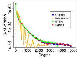
(a) Degree distribution

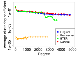
(b) Average clustering coefficient

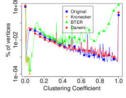
(c) Clustering coefficient

Figure 1: Comparing Darwini with Kronecker and BTER under different graph metrics on the Facebook subgraph. Darwini outperforms the other techniques in all metrics.

In this section, we evaluate different aspects of our algorithm. First, we measure the ability of the algorithm to accurately capture a number of important graph metrics, and compare our approach with state-of-the-art generative models. Second, we measure the impact of this accuracy on application-defined metrics. Finally, we evaluate the scalability of the algorithm and measure the computational overhead of our implementation.

4.1 Graph metrics

We start by measuring how accurately our algorithm re-produces a number of graph metrics, compared with the input source graph. There is a variety of metrics used to characterize graphs, here we focus on degree distribution, local clustering coefficient, joint-degree distribution as they directly characterize the structure of a graph. We also measure the PageRank distribution, Eigenvalues, K-Core decomposition, and Connected Components as higher-level metrics.

4.1.1 Degree distribution

Here, we measure how accurately Darwini reproduces the degree distribution, compared with other techniques. We first evaluate the algorithm using a portion of the Facebook social network as the source graph. Specifically, we use a subgraph of the Facebook social graph that represents a specific geographic region with approximately 3 million vertices and 700 million edges . Here, we compare Darwini with the BTER and Kronecker models as they are the only models we could evaluate for a graph of this size.

In Figure 1(a), we compare the degree distribution achieved by the different models with that of the original graph. First notice, that the Kronecker model fails to re-produce the degree distribution, as the Facebook graph does not follow the power-law model. Even though BTER provides a better approximation of the degree distribution than Kronecker, it fails to create high-degree vertices. As the algorithm tries to connect high-degree nodes to achieve the right clustering coefficient, it fails to find enough candidates. Darwini, instead, produces a degree distribution that is close to the original for all values of node degree.

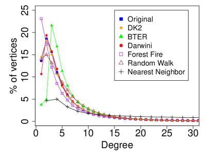
(a) Degree

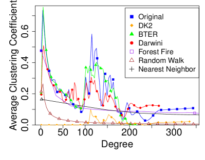
(b) Avg. clustering coefficient

Figure 2: Comparison with several models on the DBLP graph.

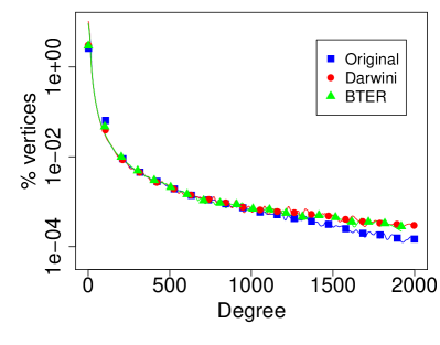
(a) Degree

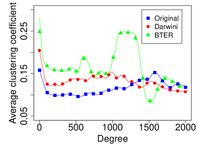
(b) Avg. clustering coefficient

Figure 3: Comparing Darwini and BTER on the Twitter graph.

Next, we repeat the same experiment on the DBLP co-authorship graph [31]. Due to the more manageable size of the DBLP, we were able to fit and generate all the models described in [23] using the publicly available implementation [3]. Here, we evaluate the best performing models among them, namely Nearest Neighbors [28], Random Walk [28], dK-2 [20] and Forest Fire [19].

Graph	Degree	Clustering Coefficient
BTER	0.21	0.64
Darwini	0.007	0.19
DK-2	0.002	6.04
Forest Fire	0.041	0.27
Random Walk	0.039	1.11
Nearest Neighbor	6.04	9.83

Table 2: KL-Divergence of degree and clustering coefficient distributions for the DBLP graph.

In Figure 2(a), we plot the actual distribution and in Table 2 we measure the Kullback-Leibler (KL) divergence between the source and the generated distributions for the DBLP graph. Consistent with the results of [20], dK-2 performs the best among this set of models. Nearest Neighbors, one of the best performing models measured in [20], here tends to produce less low-degree vertices than expected. BTER exhibits the same problem, failing to create high-degree vertices. Notice that Darwini exhibits this problem too for this a graph, but to a lesser extent. Overall, Darwini produces the second best degree distribution among all in terms of the KL-divergence.

We perform the same measurement on the Twitter follower graph [16]. Here, we compare only Darwini and BTER. Figure 3 shows the results. Both approaches produce a similar degree distribution, though the produce more high degree nodes than the original distribution. However, Darwini produces a clustering coefficient distribution that is closer to the original graph than BTER.

4.1.2 Clustering coefficient distribution

Here, we use the same graphs as above to compare the accuracy of the generated clustering coefficient. First, we measure the average clustering coefficient as a function of the vertex degree for the different models. We show the result for the Facebook graph in Figure 1(b).

Kronecker underestimates the per degree average clustering coefficient by up to 4 orders of magnitude. BTER performs better than Kronecker as it by design attempts to produce a graph with a high average clustering coefficient. Even so, notice the clustering coefficient diverges significantly for high-degree nodes. Specifically, for nodes with degree higher than 2500, the clustering coefficient could by off by an order of magnitude. Again, BTER cannot produce vertices with high degrees. Instead, for Darwini the average clustering coefficient differs follow closely the source distribution across the entire spectrum of degrees.

Figure 2(b) compares the per degree average clustering coefficient between Darwini and the rest of the models on the DBLP graph. While in terms of degree distribution the other models produced good results, most of the models underestimate the average clustering coefficient by at least X%. Only BTER can capture the average clustering coefficient. Still, Darwini outperforms BTER especially for high-degree vertices. Interestingly, the source DBLP graph exhibits an increase in the clustering coefficient for vertices with degrees between 100 and 160. Both Darwini and BTER are able to reproduce this artifact.

Further, for the Facebook graph, we also measure the distribution of the clustering coefficient values across the entire graph. We show this result in Figure 1(c). the clustering coefficient distribution. As expected, Kronecker produces only vertices with low clustering coefficient. BTER tends to produce many vertices with high clustering coefficient. Darwini captures the actual source distribution better than all models.

4.1.3 Joint degree distribution

Darwini tries to produce a realistic joint-degree distribution. Here, we measure how close to the original Facebook graph the generated joint-degree distribution is for Darwini, BTER and Kronecker. In Figure 4, we demonstrate the joint-degree distribution for vertices with degree 5, 32 and 500.

First notice that the distribution produced by Kronecker diverges the most from the original one. The BTER model improves upon Kronecker, but still produces a skewed joint degree distribution. This is due to grouping only vertices with the same degree into the same block. As a result, more vertices with same degree are connected to each other than in the original graph. Instead, by grouping vertices into the bucket based on the value of the $c_{i}d_{i}(d_{i}-1)$ product, Darwini allows the connection of more diverse vertices with respect to degree.

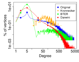
(a) Degree 5

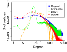
(b) Degree 32

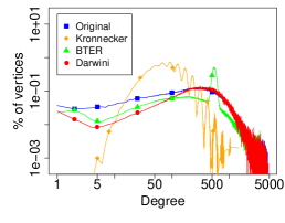
(c) Degree 500

Figure 4: Joint degree distribution on the source Facebook graph and the graphs generated by Darwini, BTER and Kronecker.

Distribution	Kronecker	BTER	Darwini
Degree	3.82	0.02	0.0014
Joint Degree, d=5	N/A	0.57	0.11
Joint Degree, d=32	0.48	0.27	0.17
Joint Degree, d=500	1.56	0.34	0.012

Table 3: KL-divergence between the original Facebook graph and the generated graph distributions.

We also measured the KL-divergence of the joint-degree distributions between the original graph and generated graphs. The result, shown in Table 3, verifies that Darwini produces a more accurate distribution. Notice that for degree $d=5$, we cannot estimate the KL-divergence for the Kronecker model as it does not produce enough vertices with this degree.

4.1.4 PageRank distribution and eigenvalues

The PageRank distribution and graph eigenvalues are common metrics used to characterize a graph structure. In Figures 5(a) and 5(b), we compare the PageRank distributions between Darwini, BTER and Kronecker, while Figure 5(c) shows the eigenvalues of the original and the generated graphs.

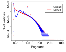
(a) PageRank

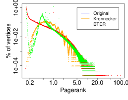
(b) PageRank

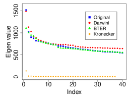
(c) Eigenvalues

Figure 5: PageRank and Eigenvalues on the source Facebook graph and the graphs generated by Darwini, BTER and Kronecker.

Although graphs generated by Darwini exhibit better PageRank distributions than other models, notice that the distribution has a significant dip caused by the block structure created at the initial stage. We hypothesize that this is due to the fact that real graphs have more hierarchical and overlapping community structure, while Darwini strictly assigns every vertex to one community. Further, notice that both BTER and Darwini generate graphs with similar distribution of eigenvalues. Darwini tends to overestimate the values at the tail of the eigenvalue spectrum.

4.1.5 K-Core decomposition

(a) Original

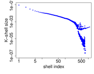
(b) Darwini

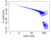
(c) BTER

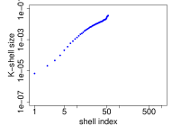
(d) Kronecker

Figure 6: K-Core decomposition on the source Facebook graph and the graphs generated by Darwini, BTER and Kronecker.

The K-core decomposition of a graph is typically used to study hierarchical properties of a graph such as finding regions of high centrality and connectedness. The K-Core decomposition is computed by recursively eliminating weakly connected vertices, and is measured by the size of the shells obtained through this recursive elimination [7]. In Figure 6, we plot the shell sizes of the original and the generated graphs.

The K-core decomposition of Darwini is the closest to that of the original graph. The difference in shell size for high shell indexes can be attributed to the block structure, in particular, the fact that each vertex belongs to a single block, while in the real graph vertices belong to multiple hierarchical and overlapping communities.

4.1.6 Connected components

Real graphs usually contain a giant connected component and a number of small components. Here, we evaluate the ability of Darwini to capture this property, and compare with BTER and Kronecker. Table 4 shows the number of components and the size of the giant component as a percentage of the total graph size. Darwini produces a giant components with a similar size and a set of small components. This holds true for BTER as well, while the Kronecker model tends to produce 1 or 2 connected components.

Generator	#components	Size of GC
Original graph	11K	99.33%
Kronecker graph	2	99.86%
BTER	27K	98.1%
Darwini	2.3K	99.83%

Table 4: Number of connected components and the relative size of the giant connected component in the original and the generated graphs.

4.2 Impact on applications

One of our initial motivations was to use Darwini to allow researchers to benchmark graph processing systems on a reference graph, for instance the Facebook social graph, without sharing the graph. Here, we measure how representative the synthetic graphs are in terms of the system performance.

In this experiment, we use as source a Facebook connected subgraph with 300M vertices. Using this source, we generate synthetic graphs with Darwini, BTER and Kronecker. Subsequently, we run a variety of graph mining application, developed on the Apache Giraph framework, on all these graphs and compare the observed performance of the Apache Giraph system. Here, we run four different applications: PageRank, Clustering Coefficient, Eigenvalue decomposition and Balanced Partitioning [26].

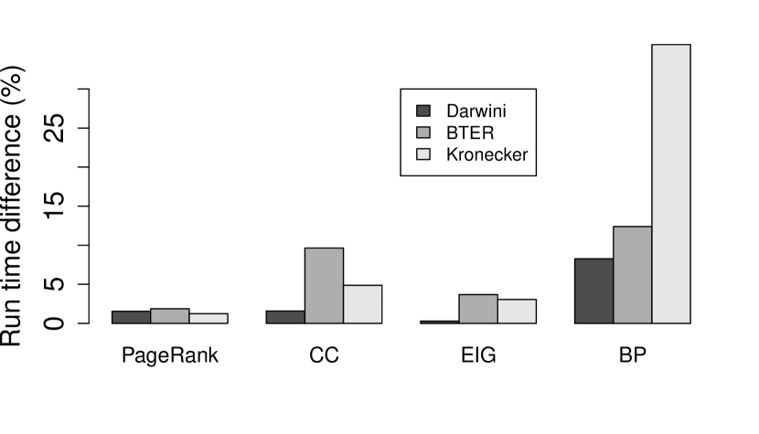
Figure 7: Impact of graph structure on system performance. The graph shows the relative performance difference compared to processing the original graph.

Figure 7 shows the relative difference in runtime between the original and the synthetic graphs for the different applications. Each data point is an average of three runs. First, notice that for PageRank the difference is small for all graphs. The computation overhead of this application is proportional to the number of edges in the graph. Giraph distributes the graph across machines randomly, therefore, the same applies for the incurred network overhead. Since all synthetic graphs have almost the same number of edges with the original graph.

The difference in performance becomes more apparent for the rest of the applications because of their computation and communication patterns. For instance, in the clustering coefficient vertex-centric algorithm, every vertex creates a message that is proportional in size to its degree and sends it to all its neighbors. Even though the number of edges is the same in all graphs, a different clustering can impact the size of the messages and, hence, the observed application performance. In these case, the observed performance on the graph generated with Darwini is closer to the one on the original graph.

4.3 Scalability

Here, we evaluate the scalability of the Darwini implementation. We use an experimental cluster with 200 machines, each with 256G of RAM and 48 cores. Figure 8(a) show the time to generate a graph as a function of the output graph size. The graph generation time scales linearly with the number of vertices until we hit the memory limit. In Figure 8(b), we show how the graph generation time improves as we increase the size of the compute cluster. For a sufficiently large graph, the time decreases linearly. Smaller graph sizes do not benefit from a large number of machines due to the network overhead.

Further, we used Darwini to generate a scaled-up version of the Facebook social graph. We used the entire Facebook social graph as the source graph and generated a synthetic graph with one trillion edges. This task took approximately 7 hours on the same 200-machine compute cluster Although we omit the details, the generated distributions are close to the source distribution, consistent with our result on the smaller subgraph.

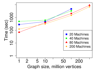
(a) Time vs. graph size

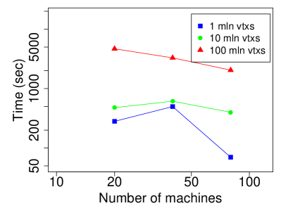
(b) Time vs. #machines

Figure 8: (a) Darwini scales linearly on the number of vertices. (b) For large graphs, Darwini scales linearly as the compute cluster size increases.

5 Related work

In this section, we briefly introduce several well-known social graph generation models.

Our work is inspired by the Block Two-Level Erdös-Rényi (BTER) [15, 25] model. As we show in our evaluation, the BTER model is capable of capturing the average clustering coefficient, but fails in generating high-degree vertices and often results in graphs with skewed joint degree distribution.

The Barabasi-Albert model [10] uses the preferential attachment mechanism to produce random graphs with power-law degree distributions. However, preferential attachment does not generally produce higher than random number of triangles, resulting in graphs with low clustering coefficient.

The Random Walk model [28] simulates the randomized walk behavior of friend connections in a social network. Each node performs a random walk starting from a randomly chosen node in the graph, and randomly connects to a new node with a given probability. The Nearest Neighbor model [28] is based on idea that people sharing a common friend are more likely to become friends. Therefore, graph generation goes as follows: after a new node is connected to an existing node, random pairs of the 2-hop neighbors are also connected with specified probability. While Random Walk and Nearest Neighbor models are relatively accurate in terms of degree distribution and clustering coefficient, they are biased towards inter-connecting high-degree nodes, and produce graphs with significantly shorter path lengths and network diameter [23].

Kronecker graphs [18] are generated by recursive application of Kronecker multiplication to an initiator matrix. The initiator matrix is selected by applying the KronFit algorithm to the original graph. Modifying the size of the initiator matrix introduces a tradeoff between overhead and accuracy. Generally, increasing the size of initiator matrix results in better accuracy, but increases the fitting time. In our experimentation, we found it hard to apply the existing KronFit implementation to real size graphs.

DK-graphs [20] is a family of stochastically generated graphs that match the respective DK-series of original graph. DK-1 graphs match the degree distribution of the original graph, while DK-2 matches the joint degree distribution. DK-3 matches the corresponding DK-3 series, including the clustering coefficient of the original graph. However generating DK-3 graph using rewiring incurs very high overhead. We are not aware of any efficient algorithm that generates large DK-3 graphs.

The LDBC Social Network Benchmark[6] is based on the idea of emulating user profiles and behaviors. Although very powerful, this approach requires to specify many parameters that are hard to fit. It is also limited to friendship graphs, while we must generally be able apply this on different types of entities and relationships.

6 Conclusion and future work

This paper introduced Darwini, a scalable synthetic graph generator that can accurately capture important metrics of social graphs, such as degree, clustering coefficient and joint-degree distributions. We implemented Darwini on top of a graph processing framework, making it possible to use it on any commodity cluster. Even so, to facilitate access to large-scale datasets, apart from open sourcing Darwini, we also intend to make generated graph datasets publicly available as well.

At the same time, we believe there are interesting future directions in this area. For instance, real social network users typically belong to multilpe communities, based on workplace, university affiliation, and others, affecting the connectivity of the graph. However, Darwini and other models assign vertices to a single community. Capturing the multi-community structure will provide more accurate synthetic datasets. Furthermore, current generators focus on the graph structure, and lack models for generating metadata, such as community labels characterizing vertices, or user similarity metrics characterizing edges. Such data will enable research in a variety of areas such as community detection algorithm, without the need to share the original data and potentially compromize user privacy.

References

- [1] Beevolve twitter study. http://www.beevolve.com/twitter-statistics.
- [2] Darwini source code. https://issues.apache.org/jira/browse/GIRAPH-1043.
- [3] Graph models for online social network analysis. http://current.cs.ucsb.edu/socialmodels/.
- [4] Twitter reports third quarter 2015 results. https://investor.twitterinc.com/results.cfm.
- [5] Yahoo Webscope Program. http://webscope.sandbox.yahoo.com.
- [6] LDBC Social Network Benchmark, 2016.
- [7] J. I. Alvarez-Hamelin, et al. k-core decomposition: a tool for the analysis of large scale internet graphs. CoRR, abs/cs/0511007, 2005.
- [8] L. Backstrom, et al. Wherefore art thou r3579x?: Anonymized social networks, hidden patterns, and structural steganography. In International Conference on World Wide Web, pages 181–190, 2007.
- [9] L. Backstrom, et al. Group formation in large social networks: membership, growth, and evolution. In ACM SIGKDD ’06, Aug. 2006.
- [10] A.-L. Barabási et al. Emergence of scaling in random networks. Science, 286(5439):509–512, 1999.
- [11] P. Boldi, et al. A large time-aware graph. SIGIR Forum, 42(2):33–38, 2008.
- [12] A. Ching, et al. One trillion edges: graph processing at facebook-scale. Proceedings of the VLDB Endowment, 8(12):1804–1815, 2015.
- [13] J. E. Gonzalez, et al. Powergraph: distributed graph-parallel computation on natural graphs. In USENIX OSDI’12, Berkeley, CA, USA, 2012.
- [14] J. E. Gonzalez, et al. GraphX: Graph Processing in a Distributed Dataflow Framework. In USENIX OSDI’14, Broomfield, CO, Oct. 2014.
- [15] T. G. Kolda, et al. A scalable generative graph model with community structure. CoRR, abs/1302.6636, 2013.
- [16] H. Kwak, et al. What is Twitter, a social network or a news media? In International Conference on World Wide Web. ACM Press, Apr. 2010.
- [17] A. Kyrola, et al. Graphchi: large-scale graph computation on just a pc. In USENIX OSDI’12, Berkeley, CA, USA, 2012.
- [18] J. Leskovec, et al. Kronecker graphs: An approach to modeling networks. J. Mach. Learn. Res., 11:985–1042, Mar. 2010.
- [19] J. Leskovec, et al. Graphs over time: Densification laws, shrinking diameters and possible explanations. In ACM SIGKDD ’05, pages 177–187, 2005.
- [20] P. Mahadevan, et al. Systematic topology analysis and generation using degree correlations. In SIGCOMM’06, pages 135–146, New York, NY, USA, 2006.
- [21] G. Malewicz, et al. Pregel: a system for large-scale graph processing. In ACM SIGMOD’10, 2010.
- [22] A. Roy, et al. Chaos: Scale-out graph processing from secondary storage. In Symposium on Operating Systems Principles, pages 410–424, 2015.
- [23] A. Sala, et al. Measurement-calibrated graph models for social network experiments. In International Conference on World Wide Web, New York, NY, USA, 2010.
- [24] A. Sala, et al. Brief announcement: Revisiting the power-law degree distribution for social graph analysis. In ACM SIGACT-SIGOPS Symposium on Principles of Distributed Computing, 2010.
- [25] C. Seshadhri, et al. Community structure and scale-free collections of erdös-rényi graphs. CoRR, abs/1112.3644, 2011.
- [26] A. Shalita, et al. Social Hash: An Assignment Framework for Optimizing Distributed Systems Operations on Social Networks. In USENIX NSDI’16, 2016.
- [27] J. Ugander, et al. The Anatomy of the Facebook Social Graph. CoRR, abs/1111.4503, 2011.
- [28] A. Vázquez. Growing network with local rules: Preferential attachment, clustering hierarchy, and degree correlations. Phys. Rev. E, 67:056104, May 2003.
- [29] G. Wang, et al. Asynchronous large-scale graph processing made easy. In CIDR, 2013.
- [30] D. J. Watts et al. Collective dynamics of "small-world" networks. Nature, 393(6684):440–442, 06 1998.
- [31] J. Yang et al. Defining and Evaluating Network Communities based on Ground-truth. In IEEE International Conference on Data Mining, May 2012.