The Detection of Diffuse Extended Structure in 3C 273: Implications for Jet Power

Abstract

We present deep Very Large Array imaging of 3C 273 in order to determine the diffuse, large scale radio structure of this famous radio-loud quasar. Diffuse extended structure (radio lobes) is detected for the first time in these observations as a consequence of high dynamic range in the 327.5 and 1365 MHz images. This emission is used to estimate a time averaged jet power, $7.2\times 10^{43}\rm{~{}ergs~{}s^{-1}}<\overline{Q}<3.7\times 10^{44}\rm{~{}ergs~{}s^{-1}}$. Brightness temperature arguments indicate consistent values of the time variability Doppler factor and the compactness Doppler factor for the inner jet, $\delta\gtrsim 10$. Thus, the large apparent broadband bolometric luminosity of the jet, $\sim 3\times 10^{46}\rm{~{}ergs~{}s^{-1}}$, corresponds to a modest intrinsic luminosity $\gtrsim 10^{42}\rm{~{}ergs~{}s^{-1}}$, or $\sim 1\%$ of $\overline{Q}$. In summary, we find that 3C 273 is actually a “typical” radio loud quasar contrary to suggestions in the literature. The modest $\overline{Q}$ is near the peak of the luminosity distribution for radio loud quasars and it is consistent with the current rate of dissipation emitted from millimeter wavelengths to gamma rays. The extreme core-jet morphology is an illusion from a near pole-on line of sight to a highly relativistic jet that produces a Doppler enhanced glow that previously swamped the lobe emission. 3C 273 apparently has the intrinsic kpc scale morphology of a classical double radio source, but it is distorted by an extreme Doppler aberration.

1 Introduction

3C 273 is the nearest and brightest quasar in virtually all wavebands from radio to gamma rays. It is the prototypical quasi-stellar object and flat (radio) spectrum, core dominated radio-loud quasar. In the standard model of quasar unification, the flat spectrum, core dominated quasars are drawn from the same parent population as the lobe dominated, radio-loud quasars, but only appear core dominated due to large Doppler boosting of a highly relativistic jet as a consequence of a nearly pole-on line of sight towards the observer (Antonucci, 1993). In an effort to test the unified scheme, deep observations were performed on representatives from a large sample of compact radio sources as determined by snap shot Very Large Array (VLA) observations (Perley, 1982). The expectation was that the radio lobe on the side of the quasar in which the jet pointed towards Earth would be viewed end on and appear as a diffuse halo surrounding a bright nuclear unresolved core. The two deepest set of observations involved the VLA at 1.4 GHz (Antonucci and Ulvestad, 1985; Murphy et al., 1993). Surprisingly, the core-halo configurations were less common than expected. However, offset lobes on both the jet and counter jet sides of the nucleus or just a single offset lobe on the jetted side were often detected. There were a large number of cores with a one sided jet and no lobes, core-jet configurations, and still some naked cores. The core-jet and naked core configurations were the most curious since it was unclear how many of these quasars had diffuse emission that required a dynamic range beyond the capability of the observations in order to be detected. One of the core-jet objects was 3C 273, despite a small easterly extension half way down the jet (see our Figure 1) that was conjectured to be evidence of a radio lobe, however no diffuse emission was detected (Davis et al., 1985; Conway et al., 1993). It was proposed that 3C 273 might be intrinsically one-sided (Davis et al., 1985). The jet structure of 3C 273 has been characterized as a “nose cone”; such jets have been suggested to be magnetically confined (Komissarov, 1999). 3C 273 has also been referred to as a “naked jet”, that is one without a surrounding radio lobe (Clarke et al., 1986). One explanation for naked jet sources is that they are young. The lobes have not formed yet since there is insufficient time for the slow back flow of plasma from the hot spot to fill a cocoon (Liu et al., 1992). However, the jet in 3C 273 is more than 150,000 light years long as projected on the sky plane and is viewed nearly pole-on. Thus, the hot spot at the end of the jet is $\sim 10^{6}(c/v_{\rm{adv}})$ years old, where $v_{\rm{adv}}$ is the hot spot advance speed. 3C 273 is not a young radio source. This raises the questions, where is the lobe emission, or why is there no lobe emission?

We have pursued a program of retrieving archival observations that is based on the hypothesis that due to the extremely bright radio core and jet, the large scale morphology has exceeded the dynamic range limits of previous observations and for this reason its true nature has eluded astronomers. Detection of the lobe emission in this proto-typical quasar is fundamentally important since the Doppler enhancement is so intense that it is difficult to extricate any type of isotropic flux that could be used to estimate jet power without the enormous ambiguity imposed by Doppler beaming. Our L-band (1365 MHz) and P-band (327.5 MHz) imaging are chosen to detect the halo emission and estimate its spectral index.

The paper is organized as follows. Section 2 describes the details of the observations. The results of Sections 2 are used to estimate the long term time average jet power in Section 3. In Section 4, we estimate the Doppler factor at the base of the jet by various means and find that it is consistently determined as $\gtrsim 10$. In Section 5, we compare the radio properties of 3C 273 to the radio loud quasar population and find it to be very typical. In this paper: $H_{0}$=70 km s^-1 Mpc^-1, $\Omega_{\Lambda}=0.7$ and $\Omega_{m}=0.3$.

Figure 1: On the left hand sided is 3C 273 at 1365 MHz. The right hand side is 3C 273 at 327.5 MHz. Contours in both images are in percentage of the peak surface brightness and increase in steps of 2. The peak surface brightness and lowest contour levels are 39.7 Jy beam^-1, $\pm 0.021\%$ for the P-band image, and 32.8 Jy beam^-1, $\pm 0.011\%$ for the L-band image.

2 Observations

The L-band observations were carried out with the AB-array of the VLA on July 9, 1995 (Project ID: AR334), while the P-band observations were carried out with the VLA A-array on March 7, 1998 (Project ID: AK461). The L-band data was provided by R. Perley (Perley et al., 2016). The total on-source time was $\sim$30 mins in the L-band and $\sim$1.5 hours in the P-band. We reduced and analyzed the data using standard procedures in AIPS. The final rms noise in the 1365 MHz image was $\sim 1.2$ mJy beam^-1 and the 327.5 MHz image was $\sim 1.1$ mJy beam^-1. The baseline-based calibration task BLCAL was used to reduce the noise in the north-south direction, which arose due to the source being close to the equator. A dynamic range of $\sim 30,000$ and $\sim 40,000$ was finally achieved at the L- and P-bands, respectively. The radio images with a beam-size of $4^{\prime\prime}\times 4^{\prime\prime}$ at the L-band and $7^{\prime\prime}\times 6^{\prime\prime}$ at the P-band, are presented in Figure 1. We estimated the total and extended diffuse flux densities using the AIPS procedure TVSTAT. These were respectively, 50.3 Jy and $0.35\pm 0.04$ Jy at the L-band, and 63.3 Jy and $1.33\pm 0.13$ Jy at the P-band. Defining the radio spectral index as $F_{\nu}\propto\nu^{-\alpha}$ yields $\alpha_{327.5}^{1365}=0.93$.

3 Estimating the Long Term Time Averaged Jet Power

A method that allows one to convert 151 MHz flux densities, $F_{151}$ (measured in Jy), into estimates of long term time averaged jet power, $\overline{Q}$, (measured in  ergs s^-1) is captured by the formula derived in Willott et al. (1999); Punsly (2005):

$$\overline{Q}\approx[(\mathrm{\textbf{f}}/15)^{3/2}]1.1\times 10^{45}\left[X^{1+\alpha}Z^{2}F_{151}\right]^{0.857}\mathrm{~{}ergs~{}s^{-1}}\;,$$ (1)

$$Z\equiv 3.31-(3.65)\times$$

$$\left[X^{4}-0.203X^{3}+0.749X^{2}+0.444X+0.205\right]^{-0.125}\;,$$ (2)

where $X\equiv 1+z$, $F_{151}$ is the total optically thin flux density from the lobes.

In practice, the qualifying statement that the $F_{151}$ is the total optically thin flux density from the lobes requires a detailed study for blazars such as 3C 273. Due to Doppler boosting on kpc scales, core dominated sources with a very bright one sided jet (such as 3C 279 and most blazars) must be treated with care (Punsly, 1995). Blazars with significant emission on super-galactic scales (scales larger than the host galaxy, i.e. $>20$ kpc) typically have resolved flux that is dominated by a one-sided jet that can be predominantly a hot spot or strong knot. The best studied example in that paper was 3C 279, in which virtually all of the extended flux was in a one-sided kpc jet. It was concluded that the jet dominated one sided kpc structure was a result of strong Doppler beaming on kpc scales in blazars. Thus, the contributions from Doppler boosted jets as well as the radio cores must be removed before applying Equation (1). Previous to this study, this could not be done for 3C 273. Hence, the importance of Figure 1 and the halo flux densities derived from them in Section 2 for estimating $\overline{Q}$.

The calculation of the jet kinetic luminosity in Equation (1) depends on an empirical multiplicative factor, f, that incorporates the uncertainty that is associated with departures from minimum energy and variations in geometric effects, filling factors, protonic contributions and the low frequency cutoff (Willott et al., 1999). The quantity, f, was further determined to most likely be in the range of 10 to 20, hence the fiducial value of 15 in Equation (1) (Blundell and Rawlings, 2000). The formula is most accurate for large classical double radio sources, thus it is not applicable for sources with a linear size of less than 20 kpc which are constrained by the ambient pressure of the host galaxy. The halo size estimated from Figure 1 is 80 kpc by 120 kpc and likely represents both radio lobes, one on the jetted side (south of the core) and the other on the counter jet (un-jetted) side (north of the core). Thus, these super-galactic “lobes” seemed to be relaxed sufficiently in order to be considered consistent with Equation (1). Due to the large asymmetry on the jetted and un-jetted (counter jet) sides of the core, the kpc jet and hot spot must be considered to be strongly Doppler boosted. Figure 1 indicates that the Doppler enhancement of the jet and hot spot is at least three orders of magnitude, if we assume approximate intrinsic bilateral symmetry in the jet production. Therefore, these are not included in determination of $F_{151}$.

Alternatively, one can also use the independently derived isotropic estimator in which the lobe energy is primarily inertial (i.e., thermal, turbulent and kinetic energy) in form (Punsly, 2005)

$$\overline{Q}\approx 5.7\times 10^{44}(1+z)^{1+\alpha}Z^{2}F_{151}\,\mathrm{~{}ergs~{}s^{-1}}\;.$$ (3)

The motivation for this derivation was the X-ray data presented in Punsly (2005) and references therein. The data indicates that the energy stored in radio lobes is typically dominated by inertial energy, not magnetic field energy, contrary to the hot spots which are often near equipartition. The derivation then finds consistency with the spectral ageing estimates of Fanaroff-Riley type II (FRII) radio lobes (Liu et al., 1992). Equation (3) generally estimates $\overline{Q}$ lower than Equation(1) and is considerably less for weaker radio sources such as 3C 273. Thusly motivated, we use Equation (1) with $\mathrm{\textbf{f}}=20$ as the maximum upper bound on $\overline{Q}$ and Equation (3) is the lower bound $\overline{Q}$ in the following.

Using $\alpha_{327.5}^{1365}=0.93$ and the flux densities from Section 2, we estimate $F_{151}\approx 2.7\rm{Jy}$, for the detected halo emission. However, it is clear from Figure 1 that due to the pole-on nature of the line of sight, a major fraction of the lobe emission projected on the sky plane is coincident with the much brighter core, jet and hot spot. Thus, it is not possible to extricate the halo flux from these bright features in the overlap region. We estimate that the flux density that is “hidden” by the bright glow of these features is between 50% and 100% of the detected extended structure. By accounting for this hidden halo flux, we are also compensating for the de-boosted hot spot flux that would exist if 3C 273 lay in the sky plane, the geometric configuration for which Equations (1) and (3) are most accurate. Thus, a more accurate estimate of the extended flux in the lobes is

$$4.1\,\rm{Jy}<F_{151}<5.5\,\rm{Jy}\,.$$ (4)

Applying this estimate to Equations (1) - (3) yields

$$7.2\times 10^{43}\rm{~{}ergs~{}s^{-1}}<\overline{Q}<3.7\times 10^{44}\rm{~{}ergs~{}s^{-1}}.$$ (5)

In conclusion, the fact that the spectral index of the lobe emission is very steep, $\alpha_{327.5}^{1365}=0.93$, and is distributed over a region much larger than the host galaxy (80 kpc by 120 kpc), the lobe emission is consistent with the most important assumption of Equations (1) and (3): the radio lobes are relaxed and are filled with synchrotron cooling plasma. Thus, after removing the Doppler enhanced core, jet and hot spot emission, one expects that the estimate of $\overline{Q}$ is consistent with those performed on classical double radio sources. This would not have been true if the halo emission had not been detected.

4 The Jet Doppler Factor

The modest value of $\overline{Q}$ in Equation (5) needs to be reconciled with the large apparent broadband apparent luminosity of the jet. The spectral energy distribution (SED) of the jet has two broad components, synchrotron emission and inverse Compton emission (Abdo et al., 2010). Both components are variable and the combined apparent luminosity of the jet is $L_{\rm{app}}\sim 2-4\times 10^{46}\rm{~{}ergs~{}s^{-1}}$ (Soldi et al, 2008; Ghisellini et al., 2010; Abdo et al., 2010). This is two orders of magnitude larger than the value of $\overline{Q}$ in Equation (5). The SED is more than an order of magnitude more luminous in the sub-millimeter and mid-IR compared to 15 GHz (Abdo et al., 2010; Soldi et al, 2008). Consequently, most of $L_{\rm{app}}$ is emitted from the jet in regions that are unresolved in our radio imaging. The total apparent luminosity is Doppler enhanced relative to the intrinsic luminosity, $L_{\rm{int}}$, by the relationship, $L_{\rm{app}}=\delta^{4}L_{\rm{int}}$ (Lightman et al., 1975). The Doppler factor, $\delta$, is given in terms of $\Gamma$, the Lorentz factor of the outflow; $\beta$, the three velocity of the outflow and the angle of propagation to the line of sight, $\theta$; $\delta=1/[\Gamma(1-\beta\cos{\theta})]$ (Lind and Blandford, 1985). The discrepancy between the magnitudes of $L_{\rm{app}}$ and $\overline{Q}$ suggests an explanation in terms of large Doppler enhancement. In order to see if the result in Equation (5) has a relationship to the current state of jet production, we proceed to estimate $\delta$ by a variety of methods.

The Doppler factor can be constrained by a brightness temperature analysis. When the brightness temperature in the plasma rest frame obeys, $(T_{b})_{\rm{intr}}>10^{12}\,{}^{\circ}\,\mathrm{K}\;$, the inverse Compton catastrophe occurs (Kellermann & Pauliny-Toth, 1969; Marscher et al, 1979). In order to explain the observed radio synchrotron jet in such sources, Doppler boosting is customarily invoked. This can be used to constrain the Doppler factor in two ways. The first, we will call the “compactness brightness temperature” argument. In this case, one measures the size of the emission region in order to estimate $T_{b}$ in the observers frame. If it gets too compact then an inverse Compton catastrophe can be averted with Doppler enhancement. In Marscher et al (1979), it is argued that in order to avoid the inverse Compton catastrophe

$$\delta_{\rm{com}}^{1.2}>(1+z)^{1.2}\frac{(T_{b})}{10^{12}\,{}^{\circ}\,\mathrm{K}}\;.$$ (6)

After considering the refractive effects and substructure, it is argued that the highest frequency, 22 GHz RadioAstron observations, yields the most reliable estimates of $(T_{b})$: $(T_{b})=1.4\times 10^{13}\,{}^{\circ}\,\mathrm{K}$ (Kovalev et al., 2016; Johnson et al., 2016). Using Equation (6), we get a constraint on the compactness Doppler factor, $\delta_{\rm{com}}>10.7$.

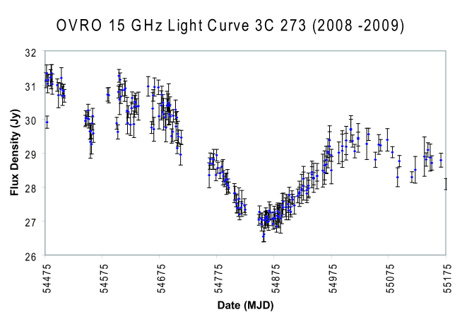
Figure 2: The 15 GHz light curve from OVRO during 2008 and 2009.

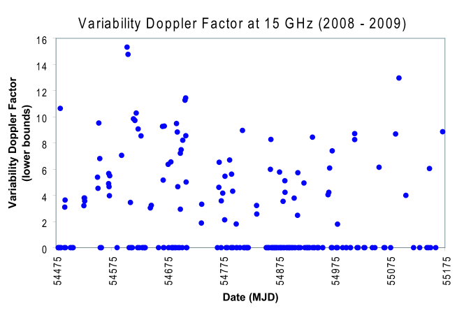
Figure 3: The measurements of the time variability Doppler factor, $\delta_{\rm{var}}$, derived from the OVRO data in Figure 2 using Equations (7) and (8). These are formally conservative lower limits.

Alternatively, one can consider the constraint on $\delta$ from flux variations, “time variability brightness temperature” arguments. The corresponding variability Doppler factor, $\delta_{\rm{var}}$ is defined as (Ghosh and Punsly, 2007; Hovata et al., 2009; Zhou et al., 2006)

$$\delta_{\rm{var}}=\left[\frac{(T_{b})_{\rm{var}}}{10^{12}\,{}^{\circ}\,\mathrm{K}}\right]^{1/3}\approx\left[\frac{8.0(1+z)}{(\nu_{o}/\mathrm{1GHz})^{2}(\Delta t_{o}/1\mathrm{yr})^{2}}Z^{2}(\Delta F_{\nu}(\mathrm{mJy}))_{o}\right]^{1/3}\;,$$ (7)

where $\Delta F_{\nu}(\mathrm{mJy})$ is the change in flux density in mJy measured at earth at frequency, $\nu_{o}$. during the time interval, $\Delta t_{o}$. The cosmological factor $Z$ was defined in Equation (2). The 15 GHz OVRO (Owens Valley Radio Observatory) light curve from 2008 to 2009 is plotted in Figure 2 (Richards et al., 2011). The measurements with large errors bars ($>0.5$ Jy) were dropped from the plot. In order to use Equation (7), we want to be cautious of false variability caused by measurement uncertainty. Thusly motivated, we subtract out this uncertainty from each flux measurement, $F_{1}\pm\sigma_{1}$ and $F_{2}\pm\sigma_{2}$ by defining a modified flux differential

$$\Delta F_{\nu}\equiv\rm{maximum}\left[\left(\mid F1-F2\mid-\sqrt{\sigma_{1}^{2}+\sigma_{2}^{2}}\right),\;0\right]\;.$$ (8)

The time sampling by OVRO is nonuniform. Our procedure was to step consecutively through the observations in temporal order. Each observation, $F_{1}$ was paired with a subsequent observation, $F_{2}$, that was as close to 10 days afterward as possible. This procedure produced over 90% of the 222 pairs of measurements with separations in time from 4 to 16 days. The resulting $\delta_{\rm{var}}$ from Equation (7) are plotted in Figure 3. It is important to note that these are lower limits. First, from a theoretical standpoint, the inverse Compton limit is the maximum possible brightness temperature. The system might actually exist well below this value (Readhead, 1994). Secondly, the reduced flux differential in Equation (8) naturally produces lower values of $\delta_{\rm{var}}$ on average in Equation (7). Thus, the high end of the distribution is most closely related to the jet Doppler factor. In conclusion, Figure 3 indicates that the jet Doppler factor is above 8 and is consistent with the estimate of $\delta_{\rm{com}}>10.7$ found above.

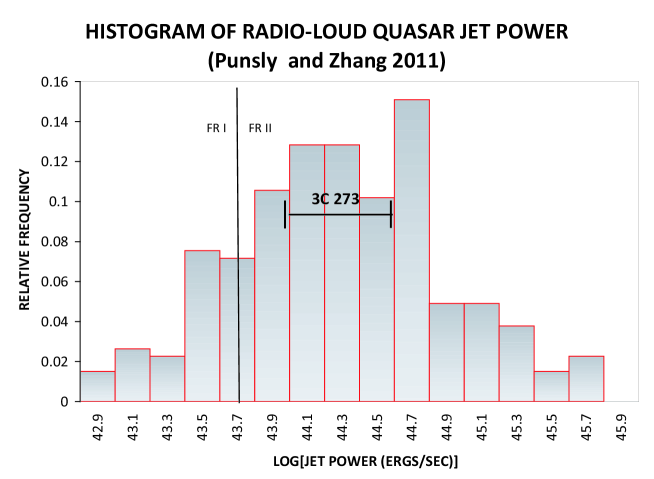
Figure 4: The long term time averaged jet power of 3C 273 compared to the distribution of jet powers for radio loud quasars.

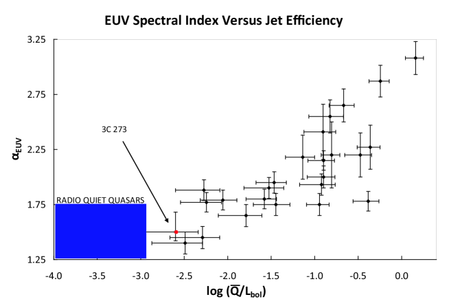
Figure 5: A scatter plot of jet efficiency, $\overline{Q}/L_{bol}$, versus $\alpha_{EUV}$ that is from Punsly et al. (2016). 3C 273 is overlayed on this plot (the red dot) for comparison.

Another consistency test of the larger values of $\delta\gtrsim 10$ is the large apparent velocity, $8<\beta_{\rm{app}}<15$, of ejected components that have been monitored with the Very Long Baseline Array (Lister et al., 2013). This is indicative of relativistic motion as well. For example, at the high end, if the jet has $\Gamma=15$ and is viewed at $3.7^{\circ}$ from the jet axis, $\delta\approx 15.5$ and $\beta_{\rm{app}}\approx 15$. More modestly, f the jet has $\Gamma=10$ and is viewed at $5^{\circ}$ from the jet axis, $\delta\approx 11.5$ and $\beta_{\rm{app}}\approx 10$. Thus, it is concluded that the preponderance of kinematical evidence consistently indicates $\delta\gtrsim 10$.

Consider a large jet Doppler factor of $\delta\gtrsim 10$ in the context of the large value of $L_{\rm{app}}\sim 2-4\times 10^{46}\rm{~{}ergs~{}s^{-1}}$. Since $L_{\rm{app}}=\delta^{4}L_{\rm{int}}$, we estimate $L_{\rm{int}}\sim 1-2\times 10^{42}\rm{~{}ergs~{}s^{-1}}$. This is implies that $L_{\rm{int}}\sim 0.01\overline{Q}$ by Equation (5). Thus, the large $L_{\rm{app}}$ of 3C 273 is consistent with the Doppler enhancement of $\sim 1\%$ dissipation of the time averaged jet power.

5 3C 273 in the Context of the Radio Loud Quasar Population

The first thing to consider is how does the value of $\overline{Q}$ for 3C 273 compare to $\overline{Q}$ of other radio loud quasars. In Figure 4, we indicate the range of values of $\overline{Q}$ for 3C 273 from Equation (5) relative to the luminosity function for $\overline{Q}$ for radio loud quasars from (Punsly and Zhang, 2011). The distribution of $\overline{Q}$, in Figure 4, is from a complete sample of optically selected low redshift quasars from the SDSS DR7 survey. The radio loud sources are all the sources that have extended emission detected by the FIRST survey on super-galactic scales. This allows us to use the estimators in Equations (1) and (3). The low redshift sample is pertinent since the corresponding FIRST radio observations are sensitive enough to detect extended flux in even the weakest FRII and many FR type I (FRI) radio sources. Being optically selected, the sample is not skewed towards sources with large radio flux densities. Figure 4 indicates that 3C 273 is typical of most radio loud quasars. The $\overline{Q}$ estimates straddle the broad maximum of the luminosity distribution.

Next, consider the jet power in the context of $L_{bol}$, the bolometric luminosity of the thermal emission from the accretion flow. From Punsly (2015), the luminosity near the peak of the spectral energy distribution at $\lambda_{e}=1100$Å (quasar rest frame wavelength), provides a robust estimator of $L_{\mathrm{bol}}$,

$$L_{bol}\approx 3.8F_{\lambda_{e}}(\lambda_{e}=1100\AA)\approx 8.9\times 10^{46}\,\mathrm{~{}ergs~{}s^{-1}}\;,$$ (9)

where the flux density is from Shang et al (2005). Note that this estimator does not include reprocessed radiation in the infrared from distant molecular clouds (Davis and Laor, 2011). There exists a strong correlation between $\overline{Q}/L_{bol}$ and the EUV (extreme ultraviolet) spectral index that has been recently demonstrated in radio loud quasars in a series of articles (see Punsly et al. (2016) and references therein). In particular, $\overline{Q}/L_{bol}$ , is correlated with the spectral index in the EUV, $\alpha_{EUV}$; defined in terms of the flux density by $F_{\nu}\sim\nu^{-\alpha_{EUV}}$ computed between 700Å  and 1100Å . The straightforward implication is that the EUV emitting region is related to the jet launching region in quasars. The EUV is the highest energy optically thick emission and likely arises near the inner edge of the accretion disk (Sun and Malkan, 1989; Szuszkiewicz et al., 1996). In order to find the location of 3C 273 in the $\overline{Q}/L_{bol}$ - $\alpha_{EUV}$ scatter plane, we first estimate $\alpha_{EUV}$ from the simultaneous FUSE (Far Ultraviolet Spectroscopic Explorer) and HST (Hubble Space Telescope) observations (Shang et al, 2005). The spectrum only goes down to 790Å  in the quasar rest frame, they fitted the continuum from 1100Å  - 790Å  with $\alpha=(1.34)^{+0.24}_{-0.11}$. The FUSE data needs to be extrapolated to 700Å  in order to compute $\alpha_{EUV}$. This is viable since the region $800\AA\,-900\AA\,$ has few if any broad emission lines in quasar spectra (Telfer et al., 2002; Stevans et al., 2014; Punsly, 2015). We estimated $\alpha=1.9\pm 0.1$ fitted to this restricted continuum . The $800\AA\,$ flux density is extrapolated to $700\AA\,$ with this spectral index in order to find $\alpha_{EUV}=(1.5)^{+0.18}_{-0.08}$. Combined with Equations (5) and (9) this yields the placement of 3C 273 in $\overline{Q}/L_{bol}$ - $\alpha_{EUV}$ scatter plane that was given in Punsly et al. (2016) and the results are shown in Figure 5. Note that 3C 273 obeys the correlation and its location in the scatter plane is typical of quasars in which most of the energy budget is dissipated as thermal emission and a relatively small fraction as a relativistic jet.

6 Conclusions

In this article, we provided an analysis of the extended emission of 3C 273 and its implications. We presented the following results

1. Radio lobes are detected for the first time in the “naked jet” quasar, 3C273. We determine the extended halo flux densities at 1365 MHz and 327.5 MHz, to be $0.35\pm 0.04$ Jy and $1.33\pm 0.13$ Jy, respectively.

2. We provide the first isotropic estimator of jet power in 3C 273. Using the halo flux, we estimate a long term time averaged jet power of $7.3\times 10^{43}\rm{~{}ergs~{}s^{-1}}<\overline{Q}<3.7\times 10^{44}\rm{~{}ergs~{}s^{-1}}$. This straddles the peak of the radio loud quasar luminosity distribution (Figure 4)

3. It is estimated, from compactness arguments with RadioAstron and time variability arguments, that the Doppler factor in the base of the jet is $\delta\gtrsim 10$, consistent with the observations of superluminal apparent motion of components $\sim 8c-15c$.

4. We use this estimate of the Doppler factor to constrain the intrinsic jet broadband (radio to gamma ray) luminosity, $L_{\rm{int}}\sim 1-2\times 10^{42}\rm{~{}ergs~{}s^{-1}}$.

5. The location of 3C 273 in the $\overline{Q}/L_{bol}$ - $\alpha_{EUV}$ plane is typical of quasars in which most of the energy budget is dissipated as thermal emission and a relatively small fraction as a relativistic jet (Figure 5).

It seems that the estimates in points 2 and 4 are compatible. The implication is that if the current jet power, $Q(t)\sim\overline{Q}$ then $\sim 1\%$ of the jet power is dissipated as radiation losses. This is a rather modest amount of dissipated power considering the propensity for constrained high velocity magnetized plasmas to generate dissipative instabilities and produce shocks; especially if the solar wind is an example (Vasquez et al., 2003; Cramer et al., 2009). From points 2, 3 and 5, 3C 273 is a prototypical radio loud quasar with an extremely large Doppler enhancement due to relativistic line of sight affects.

References

- Abdo et al. (2010) Abdo, A., Ackermann, M. Agudo. I. et al. 2010 ApJ 716 30
- Antonucci (1993) Antonucci, R.J. 1993, Annu. Rev. Astron. Astrophys. 31 473
- Antonucci and Ulvestad (1985) Antonucci, R.J. and Ulvestad, J. 1985, ApJ 294 158
- Becker et al. (1995) Becker, R. H., White, R. L., and Helfand, D. J. 1995, ApJ, 450, 559
- Blundell and Rawlings (2000) Blundell, K., Rawlings, S. 2000 AJ 119 1111
- Clarke et al. (1986) Clarke, D. Norman, M. and Burns, J. 1986, ApJL, 311, 63
- Conway et al. (1993) Conway, R., Garrington, S. Perley, R. and Biretta, J. 1993, A& A, 267, 347
- Cramer et al. (2009) Cramer, S., Matthaeus, W., Breech, B. and Kasper, J. 2009 ApJ 702 1604
- Davis et al. (1985) Davis, R., Muxlow, I., and Conway, R. 1985, Nature 318 343
- Davis and Laor (2011) Davis, S., Laor, A. 2011, ApJ 728 98
- Ghosh and Punsly (2007) Ghosh, K. and Punsly, B. 2007 ApJL 661 139
- Ghisellini et al. (2010) Ghisellini, G, Tavecchio, F. and Foschini, L. et al. 2010 MNRAS 402 497
- Gunn (1978) Gunn, J. 1978 in Observational Cosmology, Eight Advance Course, Swiss Society of Astronomy and Astrophysics, p. 26 eds A. Maeder, L. Martinet and G. Tammann (Geneva Observatory: Sauverny Switzerland)
- Hovata et al. (2009) Hovatta, T., Valtaoja, E., Tornikoski, M., & L hteenm ki, A. 2009, A&A, 494, 527
- Johnson et al. (2016) Johnson, Michael D.; Kovalev, Yuri Y., et al. 2016 ApJ 820 10
- Kellermann & Pauliny-Toth (1969) Kellermann, K. I., & Pauliny-Toth, I. I. K. 1969 ApJ,155, L71
- Komissarov (1999) Komissarov, S. 1999 MNRAS 308 1069
- Kovalev et al. (2016) Kovalev, Y. Y., Kardashev, N. S., Kellermann, K. I., et al. 2016 ApJ 820 9
- Lightman et al. (1975) Lightman, A., Press, W., Price, R. and Teukolsky, S. 1975, Problem Book in Relativity and Gravitation (Princeton University Press, Princeton)
- Lind and Blandford (1985) Lind, K., Blandford, R. 1985 ApJ 295 358
- Liu et al. (1992) Liu, R., Pooley, G., Riley, J. 1992 MNRAS 257 545
- Lister et al. (2013) Lister, M. L., Aller, M. F., Aller, H. D., et al. 2013, AJ, 146, 120
- Marscher et al (1979) Marscher, a. et al 1979, ApJ 233 498
- Murphy et al. (1993) Murphy, D., Browne, I.W.A., Perley, R.. 1993 MNRAS 264 298
- Perley (1982) Perley, R. 1982 AJ 87 859
- Perley et al. (2016) Perley, R., Röser, H.-J., Jester, S., Meisenheimer, K. 2016 in preparation
- Punsly (1995) Punsly, B. 1995 AJ 109 1555
- Punsly (2005) Punsly, B. 2005 ApJL 623 9
- Punsly (2015) Punsly, B. 2015 ApJ 806 47
- Punsly et al. (2016) Punsly, B., Reynolds, C., Marziani, P., O’Dea, C. 2016, MNRAS 459 4233
- Punsly and Zhang (2011) Punsly, B. and Zhang 2011 ApJL 735 3
- Readhead (1994) Readhead, A. 1994, ApJ 426 51
- Richards et al. (2011) Richards, J., Max-Moerbeck1, W., Pavlidou1, V. 2011, ApJS 194 29
- Scott et al. (2004) Scott, J., Kriss, G.. Brotherton, M. et al. 2004, ApJ 615, 135
- Shang et al (2005) Shang,Z., Brotherton, M. Green, R. et al. 2005 ApJ 619 41
- Soldi et al (2008) Soldi, S., T rler1, M., Paltani1,S. et al. 2008 A&A 486 411
- Stevans et al. (2014) Stevans, M., Shull, M., Danforth, C., Tilton, E. 2014ApJ 794 75
- Sun and Malkan (1989) Sun, W.-H., and Malkan, M. A 1989, ApJ 346 68
- Szuszkiewicz et al. (1996) Szuszkiewicz, E., Malkan, A., and Abramowicz, M. A. 1996, ApJ 458 474
- Telfer et al. (2002) Telfer, R., Zheng, W., Kriss, G., Davidsen, A. 2002 ApJ 565 773
- Vasquez et al. (2003) Vasquez, A., van Ballegooijen, A. and Raymond, J. 2011 ApJ 598 1361
- Willott et al. (1999) Willott, C., Rawlings, S., Blundell, K., Lacy, M. 1999 MNRAS 309 1017
- Zhou et al. (2006) Zhou, H. et al 2006 ApJ 639 716