Noninvasive imaging of 3D micro and nanostructures by topological methods

Abstract

We present topological derivative and energy based procedures for the imaging of micro and nanostructures using one beam of visible light of a single wavelength. Objects with diameters as small as $10$ nm can be located, and their position tracked with nanometer precision. Multiple objects distributed either on planes perpendicular to the incidence direction or along axial lines in the incidence direction are distinguishable. More precisely, the shape and size of plane sections perpendicular to the incidence direction can be clearly determined, even for asymmetric and non-convex scatterers. Axial resolution improves as the size of the objects decreases. Initial reconstructions may proceed by glueing together 2D horizontal slices between axial peaks or by locating objects at 3D peaks of topological energies, depending on the effective wavenumber. Below a threshold size, topological derivative based iterative schemes improve initial predictions of the location, size and shape of objects by postprocessing fixed measured data. For larger sizes, tracking the peaks of topological energy fields that average information from additional incident light beams seems to be more effective.

1 Introduction

Ideally, imaging biological samples resolves structures in three dimensions, over a wide range of scales without harming the specimen. To prevent damage, live cells have traditionally been imaged using light microscopes. Visible light corresponds to a wavelength range of $380$-$740$ nanometers (nm). Cells are large compared to the illumination wavelength, but comprise finer structures down to molecular sizes, see Table 1.

Unstained biological samples lack contrast in straightforward optical imaging. To gain contrast on structures of interest, biologists have very productively used fluorescent dyes. However, such stains are invasive, phototoxic and tend to bleach over extended periods of time [27]. For this reason, it is useful to consider techniques which can image biological structures in their native state. Living cells are almost transparent, affecting mostly the phase of light passing through them and making only minimal amplitude changes. Differential interference contrast (DIC) and phase contrast microscopes are sensitive to these phase changes [44], and have been the gold standard for optical imaging of unstained cells. More recent holographic techniques sense phase in a more quantitative manner that contains three dimensional information. While optical reconstructions reproduce an aspect of an object, digital holography recreates object data from the recorded light measurements.

Different techniques have been exploited to heighten spatial resolution of optical microscopes beyond the diffraction limit [4]. Confocal 3D imaging [41] resorts to point illumination. The need to scan an imaging point through the sample in all three dimensions limits its ability to capture fast events subjecting samples to substantial photon flux and potential photodamage. On the other hand, $4\pi$ laser scanning fluorescence microscopes [20] use two objectives to divide the diffraction limit by a factor $2$. For visible light wavelengths, this limit ranges from about $68$ nm to $132$ nm. Improved resolution (down to $10$ nm) of cellular nanostructures marked with fluorescent stains has been achieved combining spectral precision distance microscopy and spatially illuminated modulation, that blends two or three different emitted wavelengths [1, 45].

Red blood cell	Nucleus	Chloroplast	Mitochondrion
9 $\mu$m	6 $\mu$m	5 $\mu$m	3 $\mu$m
Bacterium E. Coli	Membrane	Protein	Virus
2 $\mu$m	3-10 nm	10 nm	5-300 nm

Table 1: Size of cells and cellular elements.

Holographic techniques provide a noninvasive alternative for high speed 3D live cell imaging [38, 50]. Holograms can be recorded as fast as cameras permit, usually in the millisecond or microsecond range, and the process does not damage samples. An hologram is not an image, but an encoding of the light field as an interference pattern, with information about both the intensity and the phase of the light field [46]. Holograms can be decoded optically or numerically. Digital holography is devoted to the numerical reconstruction of digitally recorded holograms [31, 50]. Numerical processing of the encoded information allows us to compute simultaneously the phase and the intensity of the propagated wave field. It also makes it possible to focus on different object planes without resorting to optomechanical motion [49, 54], and postprocess the information to improve resolution and remove aberrations [24, 34]. Resolution can be further enhanced by combining light incoming from different directions [33]. Inverse scattering analysis is employed in Ref. [51] to track the dynamics of wavelength-scale particles with nanometer-scale precision and millisecond temporal resolution. These inverse scattering techniques are computationally intensive, but this burden can be reduced without loss of resolution by using a smaller number of randomly arranged detectors, as discussed in Ref. [15]. Progress in digital holography is strongly related to advances in the mathematical techniques to decode light measurements. In this paper, we demonstrate the potential of topological methods for the noninvasive imaging of low contrast structures displaying a variety of lengths in the nano and microscales using light measurements in holographic settings.

Topological methods recast the inverse light scattering problem as a constrained optimization problem and analyze the potential of the topological energy and the topological derivative of the resulting shape functional to image the objects. To simplify, we assume that measurements of the full light wave field $E$ are available at set of detectors, see Fig. 1. The magnitude actually measured in holograms is $|H|^{2}=|E+R|^{2}=|E|^{2}+E\overline{R}+\overline{E}R+|R|^{2}$, where $R$ is an independent reference light beam, assumed to be a uniform plane wave, whereas $E$ is the wave field generated when the incident light $E_{inc}$ interacts with the object. Notice that the quantity we are interested in is $E$, the complex (magnitude and phase) electric field. When imaging biological or similar samples, reasonable approximations might allow one to extract the electric field from the recorded hologram. For example, for inline holography, we first normalize by the constant reference field:

$$\left|\frac{H}{R}\right|^{2}=1+\frac{E}{R}+\frac{\overline{E}}{\overline{R}}+\left|\frac{E}{R}\right|^{2}.$$ (1)

Since cells and many other objects we are interested in imaging are weak scatterers, it is a reasonable approximation to neglect the $|E/R|^{2}$ term. Thus we can write:

$$\left|\frac{H}{R}\right|^{2}-1\approx\frac{E}{R}+\frac{\overline{E}}{\overline{R}}.$$ (2)

Effective algorithms to extract the total field $E$ from approximation (2) are yet to be devised. We assume here that $E$ is known at the detectors.

Topological derivative based methods have been implemented in many inverse scattering problems, see [6, 8, 10, 23, 28, 29] for applications in acoustics, elasticity, fluids and tomography, for instance, usually in two-dimensional settings. They have the ability of providing first guesses of objects in absence of any a priori information. Such approximations can then be improved by iterative schemes, as we will discuss later. The performance of topological derivatives usually varies with the wavenumber, as observed in acoustic scattering problems. For small wavenumbers, regions where topological derivatives take large negative values mark object locations. As the wavenumber increases, the topological derivative fields develop oscillations. Remarkably, for large wavenumbers and two-dimensional problems, large negative values mark the boundary of single objects when a wide distribution of incident waves and receptors is considered [5]. Moreover, for large wavenumbers and in three dimensions, topological derivative fields that average information provided by incident waves from all possible directions allow us to reconstruct the boundary of isolated convex objects [30]. However, handling multiple or non-convex objects becomes a challenge. To tackle difficulties caused by oscillatory behavior, topological derivatives have been replaced by topological energies in two-dimensional time-dependent wave scattering [17].

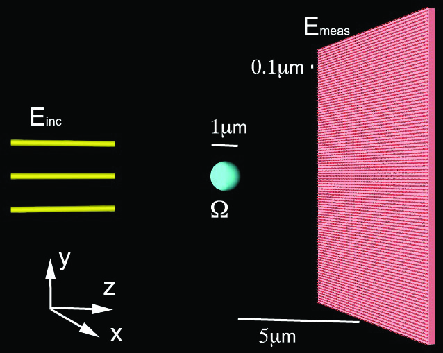
Figure 1: Imaging setting. An object $\Omega$ is illuminated by a light beam $E_{inc}$. The total field $E$ is measured at a grid of detectors placed on a screen, orthogonal to the beam direction $z$. Typical sizes for the object range from $2\,\mu{\rm m}$ to $10$ nm. Its distance to the screen is about $5\,\mu{\rm m}$. The screen size is $10\,\mu{\rm m}\times 10\,\mu{\rm m}$. The step for the grid of detectors is $0.1\,\mu{\rm m}$. Detectors correspond to a CMOS camera pixels [47].

In this paper we mostly consider a single incident direction because that corresponds to the way optical microscopes are conventionally built. It would be possible for a custom built microscope to use some range of incident directions, but that be fairly sharply limited by the numerical aperture of the observing objective lens. Here, we consider time-harmonic light scattering in three dimensions (3D) in the imaging setting represented in Figure 1. The wavenumbers in our specific imaging setting, detailed in Sections 2 and 4, lie in the transition to large wavenumbers. To overcome difficulties created by the aforementioned oscillatory behavior of the topological derivative, we analyze information from both topological energies and topological derivatives. We are able to locate multiple three-dimensional objects and spot the shape of non-convex and asymmetric objects, down to spatial scales of a few nanometers using just one incident wave and one detector screen. Objects in the shadow of other objects in the light direction are clearly distinguished. As the size of the objects varies, a transition in the behavior of the topological fields is observed. For sizes below a micron, objects are located at peaks of these 3D fields. For larger sizes this remains true only in lateral 2D slices. On axial 2D slices, the topological fields concentrate at the edges, before and past the object. Interestingly, some holographic reconstruction procedures show that the brightest points become focal caustics of objects as they get larger. Essentially the object can behave as a lens, and such reconstructions pick out the bright point where the object brings the light into smaller focus [12, 16]. A similar effect might be occurring with topological fields here. Ref. [30] contains a further theoretical discussion assuming impenetrable defects and short wavelengths.

Proposing a deterministic (no or minimal human input needed) algorithm for turning topological fields into 3D models of objects would be of great value. For small enough objects, we are able to improve a first guess of the scatterers employing an iterative procedure that postprocess the same measured data. On the contrary, our preliminary tests suggest that objects larger than the wavelength are better resolved by considering additional incident waves. From the computational point of view, implementing iterative schemes involving shapes requires overcoming a number of nontrivial technical issues about how to generate and mesh the topological field based three-dimensional approximations of the obstacle. Such approximations must be designed to adjust objects defined by the knowledge of which points of a three-dimensional cubic grid lie inside and outside. We propose a way to deal with this problem which is well suited for some coupled finite element-boundary element solvers. Future work could investigate how much can be gained by varying incident waves within the acceptance angle of the objective accounting for the asymmetric loss of high frequency information along the displaced angle.

Topological field based methods provide first guesses of objects in absence of a priori information, other than the measured data, the incident waves, and the material parameters of the background medium. They locate abrupt changes in the nature of the medium. Once an initial guess of the contours of the scatterers is available, we have two choices. First, we may assume that their material parameters are known and seek to improve the knowledge of their geometry. This can be done by topological field based iterative schemes [6], as discussed above, or employing other reconstruction methods to track sharp interfaces in the parameter values (identified with contours of objects), such as level sets [18, 19] or contour deformations [10]. Both are often initialized using topological derivatives. If the material parameters of the anomalies are unknown, we may combine these techniques with gradient methods to approximate the spatial variation of such parameters within the objects [7, 8]. Alternatively, we may apply from the beginning strategies to reconstruct the parameter profile distribution everywhere. 2D studies in an electric impedance tomography setting [8] suggest that first defining object boundaries with topological derivative methods and then approximating spatial variations of the unknown object parameters with a gradient technique is more efficient than employing the simple gradient technique to reproduce spatial variations everywhere from the beginning. In microwave imaging with sources distributed all around the objects, sophisticated iterative minimization schemes yield good reconstructions of permittivity profile distributions in a number of specific tests [9, 11, 22, 36, 52, 53] for objects smaller than the wavelength. They are all Newton type algorithms. Linear sampling has also been exploited to reproduce the morphology of these targets surrounded by sources [9]. In our setting, we are restricted to one source, as mentioned above, and the refractivity indexes (therefore the objects permittivities) are often known. However, it would be of interest to investigate the performance of these Newton schemes combined with topological methods for an analysis of the permittivity profiles within the objects, as it might help to resolve structures in more detail.

In our imaging setting, considering multiple frequencies in the visible light range does not seem to produce significative improvements over working with one, as deduced from the numerical simulations we have performed so far. On the contrary, averaging information from multiple frequencies has been shown to enhance precision in 3D microwave imaging [52] and 2D acoustic applications [25, 40]. Let us emphasize that, in holography, light detectors are placed past the objects, whereas in underground acoustic imaging, for instance, emitters and receptors are usually placed on the same surface. In microwave imaging, sources are often distributed all around the object while receivers are restricted to a circle around it. These variations strongly affect the oscillatory structure of the resulting three-dimensional topological derivative and topological energy fields.

The paper is organized as follows. Section 2 describes the imaging setting and formulates the associated constrained optimization problem. Section 3 introduces topological derivatives and energies as effective tools in the imaging of cellular structures using visible light. Section 4 illustrates the ability of these techniques to track the size, shape and location of three-dimensional rods and balls of varying size, as well as multiple, non-convex and asymmetric objects. Section 5 develops iterative strategies to improve the initial reconstructions. We discuss the procedures used to construct three-dimensional approximations of the obstacles and to solve the auxiliary boundary value problems for wave fields. Section 6 illustrates how predicted shapes may improve depending on their size, either by iteration or by adding incident waves. Finally, Section 7 summarizes our conclusions.

2 Inverse scattering problem

We plan to image objects of cell size using light. Cells and cell structures have usually sizes in the micrometer range ($1\,\mu$m= $10^{-6}$ m= $10^{3}$ nm), see Table 1. As mentioned earlier, the ability of an imaging system to resolve detail is ultimately limited by diffraction (interference of waves when a wave encounters an obstacle comparable in size to its wavelength). The resolution of light microscopes is limited by the wavelength of visible light, which is in the range $400-700$ nm. According to Table 1, this should make possible to visualize cells, and some structures within the cell, such as the nucleus, mitochondria and chloroplasts. On the contrary, to resolve for viruses or finer cell details enhanced resolution is needed. Similarly, the cell membrane is only about $3-10$ nm and cannot be resolved with standard light microscopes. Bacteria usually do not have any membrane-wrapped organelles (e.g., nucleus, mitochondria, endoplasmic reticulum), but they do have an outer membrane.

(a)                                            (b)
         

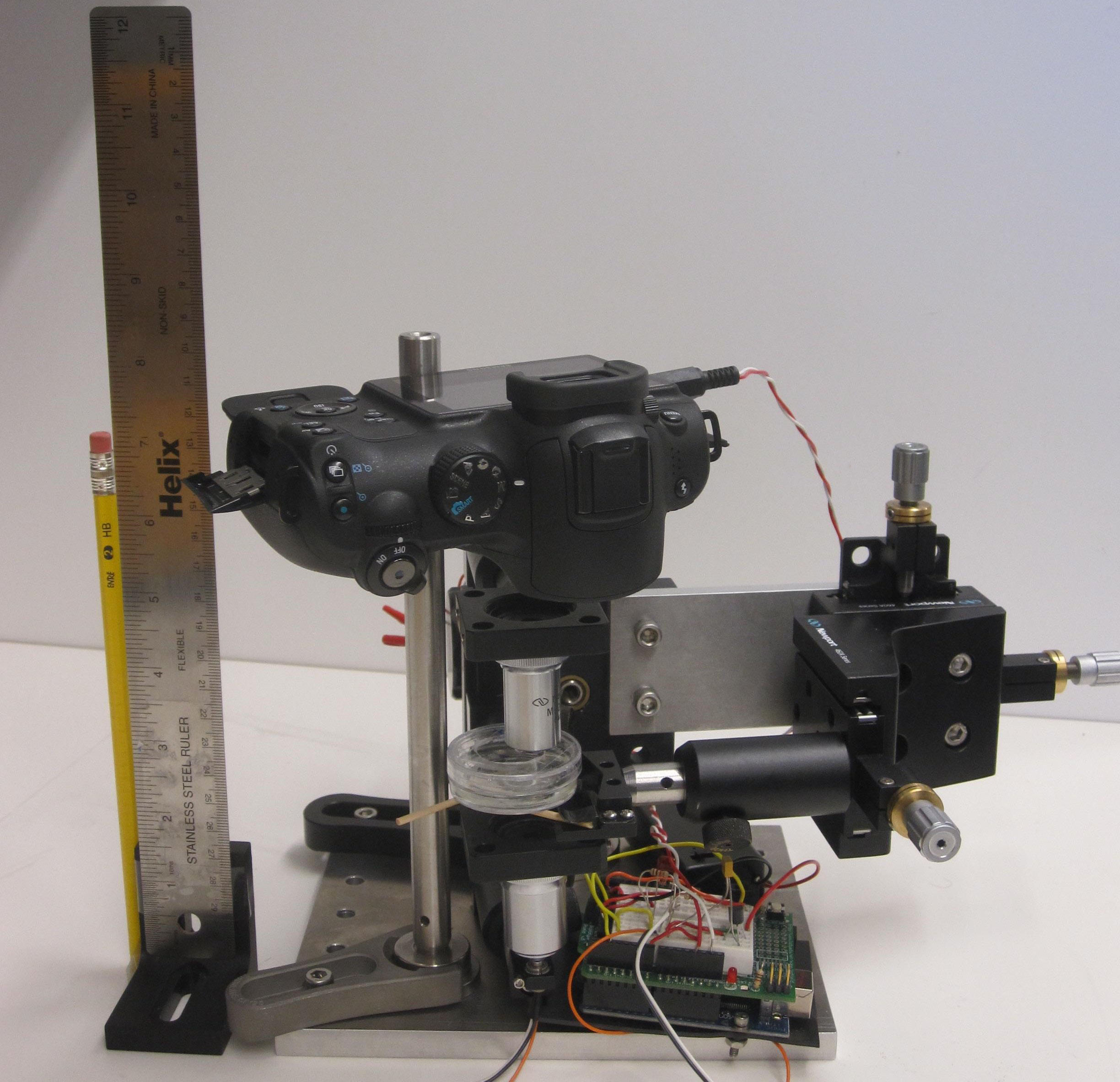
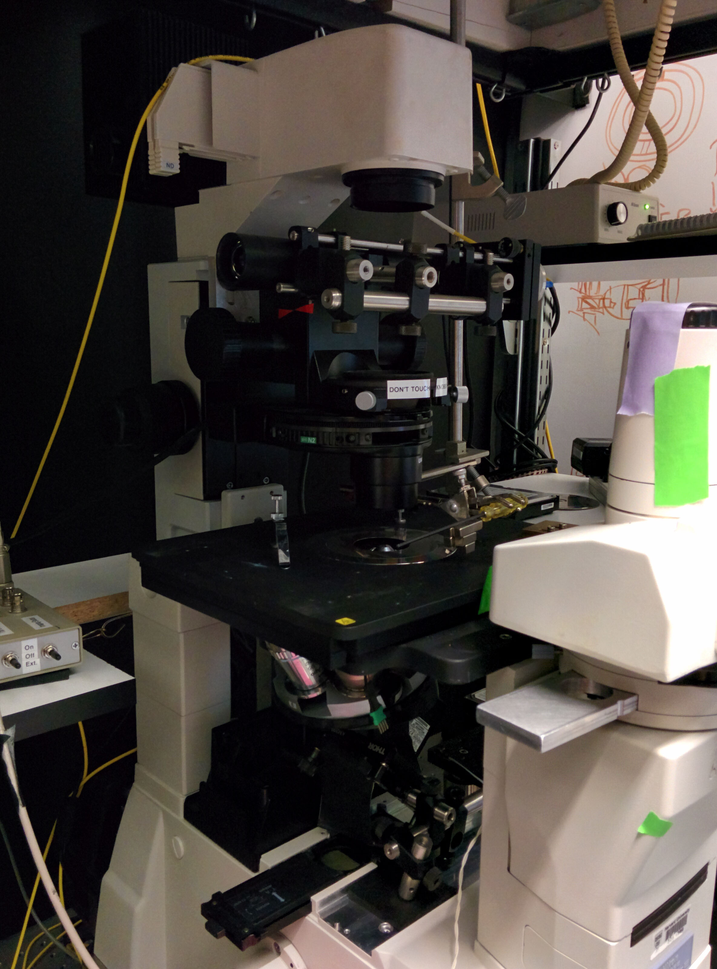
Figure 2: Holographic microscopes used for biological and soft matter imaging at Harvard University. (a) Small, self-contained, battery powered microscope for portable and in incubator use (b) Full-size, high precision microscope with optical trapping and conventional imaging capabilities.

The imaging setting is depicted in Figure 1. Holographic microscopes based on a similar setting are shown in Figure 2. In such settings, cells are placed near a screen illuminated by an incident wave ${\cal E}_{inc}$. Part of the incident wave is transmitted inside the objects $\Omega$, and the rest is scattered. The evolution of the light wave field

$${\cal E}(\mathbf{x},t):=\left\{\begin{array}[]{ll}{\cal E}_{inc}(\mathbf{x},t)+{\cal E}_{sc}(\mathbf{x},t),&\quad\mbox{$\mathbf{x}\in\mathbb{R}^{3}\setminus\overline{\Omega}$},\ \ t>0,\\ {\cal E}_{tr}(\mathbf{x},t),&\quad\mbox{$\mathbf{x}\in\Omega$},\ \ t>0,\end{array}\right.$$

is governed by a wave equation

$$\varepsilon(\mathbf{x}){\cal E}_{tt}(\mathbf{x},t)-{\rm div}({1\over{\mu(\mathbf{x})}}\nabla{\cal E}(\mathbf{x},t))=0,$$ (3)

where $\varepsilon$ is the permittivity and $\mu$ is the permeability. Electromagnetic wave equations are used to fit real holograms in references [26, 32, 35, 42, 51]. The electric field scattered by spherical particles is computed exactly using the Mie solution in [32, 35], and extensions of the Mie solution to multiple particles in [26, 42]. Reference [51] exploits the DDA (discrete dipole approximation) to solve the wave equation for more general shapes and resorts to less sophisticated inversion techniques to work with real holograms of simple objects.

If we assume that $\varepsilon$ and $\mu$ are constant inside the exterior medium and inside the objects $\Omega$,

$$\varepsilon(\mathbf{x})=\left\{\begin{array}[]{ll}\varepsilon_{e},&\quad\mathbf{x}\in\mathbb{R}^{3}\setminus\overline{\Omega},\\ \varepsilon_{i},&\quad\mathbf{x}\in\Omega,\end{array}\right.\qquad\mu(\mathbf{x})=\left\{\begin{array}[]{ll}\mu_{e},&\quad\mathbf{x}\in\mathbb{R}^{3}\setminus\overline{\Omega},\\ \mu_{i},&\quad\mathbf{x}\in\Omega,\end{array}\right.$$

we have wave equations of the form

$${\cal E}_{tt}-c^{2}\Delta{\cal E}=0,$$ (4)

with constant wave speeds $c_{e}={1\over\sqrt{\varepsilon_{e}\mu_{e}}}$ in the exterior medium $\mathbb{R}^{3}\setminus\overline{\Omega}$ and $c_{i}={1\over\sqrt{\varepsilon_{i}\mu_{i}}}$ inside $\Omega$. If we further assume that the incident wave is time-harmonic,

$${\cal E}_{inc}(\mathbf{x},t)=\mbox{Re}[e^{-2\pi\imath\nu t}E_{inc}(\mathbf{x})],$$

where $\nu$ is the frequency of the light wave (in Hz or cycles/second), then, the wave field $\cal E$ is time-harmonic as well, ${\cal E}(\mathbf{x},t)=\mbox{Re}[e^{-2\pi\imath\nu t}E(\mathbf{x})]$, and we arrive at the following stationary problem for the (complex) amplitude $E(\mathbf{x})$:

$$\left\{\begin{array}[]{ll}\Delta E+\big{(}\frac{2\pi\nu}{c_{e}}\big{)}^{2}E=0,&\quad\mbox{in $\mathbb{R}^{3}\setminus\overline{\Omega}$},\\ \Delta E+\big{(}\frac{2\pi\nu}{c_{i}}\big{)}^{2}E=0,&\quad\mbox{in $\Omega$},\\ E^{-}=E^{+},&\quad\mbox{on $\partial\Omega$},\\ \frac{1}{\mu_{i}}\,\partial_{\mathbf{n}}E^{-}=\frac{1}{\mu_{e}}\,\partial_{\mathbf{n}}E^{+},&\quad\mbox{on $\partial\Omega$}.\end{array}\right.$$ (5)

The superscripts “$+$” and “$-$” at the transmission conditions on the boundary $\partial\Omega$ denote limits from the interior and the exterior of $\Omega$ respectively, and $\partial_{\mathbf{n}}$ stands for normal derivatives, with $\mathbf{n}$ pointing outside $\Omega$. The problem is completed with the standard Sommerfeld radiation condition at infinity,

$$\lim_{r:=|\mathbf{x}|\to\infty}r\big{(}\partial_{r}(E-E_{inc})-\imath\frac{2\pi\nu}{c_{e}}(E-E_{inc})\big{)}=0,$$ (6)

modeling that only outgoing waves are allowed, that is, waves are not scattered from infinity.

For simplicity, wave amplitudes and distances are nondimensionalized in terms of a reference length $L$. Since we plan to use incident waves of different frequencies (therefore associated to different wavelengths), we choose a reference length of the order of magnitude of the size of the objects we wish to locate: $L=1\,\mu$m. Setting $\mathbf{x}^{\prime}:=\mathbf{x}/L$, $E^{\prime}:=E/a$ (the factor $a$ represents the units of the electric field) and using the notation

$$\Omega^{\prime}:=\Omega/L,\qquad E^{\prime}(\mathbf{x}^{\prime}):=E(\mathbf{x})/a,\qquad E^{\prime}_{inc}(\mathbf{x}^{\prime}):=E_{inc}(\mathbf{x})/a,$$

and the dimensionless parameters

$$\beta:=\frac{\mu_{e}}{\mu_{i}},\qquad k_{e}:=\frac{2\pi\nu L}{c_{e}},\qquad k_{i}:=\frac{2\pi\nu L}{c_{i}},$$ (7)

problem (5)–(6) is written as:

$$\left\{\begin{array}[]{ll}\Delta E^{\prime}+k_{e}^{2}E^{\prime}=0,&\quad\mbox{in $\mathbb{R}^{3}\setminus\overline{\Omega^{\prime}}$},\\ \Delta E^{\prime}+k_{i}^{2}E^{\prime}=0,&\quad\mbox{in $\Omega^{\prime}$},\\ (E^{\prime})^{-}=(E^{\prime})^{+},&\quad\mbox{on $\partial\Omega^{\prime}$},\\ \beta(\partial_{\mathbf{n}}E^{\prime})^{-}=(\partial_{\mathbf{n}}E^{\prime})^{+},&\quad\mbox{on $\partial\Omega^{\prime}$},\\ \displaystyle\lim_{r:=|\mathbf{x}^{\prime}|\to\infty}r\big{(}\partial_{r}(E^{\prime}-E^{\prime}_{inc})-\imath k_{e}(E^{\prime}-E^{\prime}_{inc})\big{)}=0.\end{array}\right.$$ (8)

The magnetic permeability of tissues is almost the same as in the free space $\mu_{0}$, and does not change with frequency [37]; therefore, we set $\beta=1$.

We work with laser lights of wavelengths $405$ nm (violet) and $660$ nm (red), in the lower and upper limits of the visible wavelength range. The corresponding frequencies are $7.38e14$ Hz for light of wavelength $405$ nm and $4.5e14$ for $660$ nm light. The selected wave speeds are $c_{e}=2.25e8\,{\rm{m\over s}}$ in the background medium and $c_{i}=2.15e8\,{\rm{m\over s}}$ or $c_{i}=1.87e8\,{\rm{m\over s}}$ inside the objects. These choices yield the dimensionless reference wavenumbers collected in Table 2 for a reference length $L=1\,\mu{\rm m}$. We will fix these values in the numerical simulations for different object sizes ${\cal L}$. However, each simulation has ‘effective’ dimensionless wavenumbers ${\cal K}_{e}=k_{e}{\cal L}/L$ and ${\cal K}_{i}=k_{i}{\cal L}/L$.

	Violet light ($405$ nm)	Red light ($660$ nm)
$k_{e}$ (background medium)	$20.60$	$12.56$
$k_{i}$ (lipid membranes)	$24.79$	$15.12$
$k_{i}$ (organelles, nucleus)	$21.56$	$13.15$
$\beta$	1	1

Table 2: Dimensionless parameters for the model.

To image the object $\Omega$, we locate a mesh of detectors $\{\mathbf{x}_{1},\dots,\mathbf{x}_{N}\}$ on a plane screen $\Pi_{meas}$ that is illuminated by a plane time-harmonic incident wave in the direction $\mathbf{d}$ orthogonal to the screen. To simplify, we assume that $\mathbf{d}=(0,0,1)$ (see Figure 1). Mathematically, this is modeled by

$$E_{inc}(\mathbf{x})/a=E^{\prime}_{inc}(\mathbf{x}^{\prime})=E^{\prime}_{inc}(x^{\prime},y^{\prime},z^{\prime})=e^{\imath k_{e}z^{\prime}}.$$

The total field $E$ is then measured at the detectors, obtaining the set of data $E_{meas,j}$ for $j=1,\dots,N$. The measured data encode information about the position, structure, size, and shape of $\Omega$. Extracting this information from the data constitutes the inverse problem to be solved: find the object $\Omega$ such that

$$E(\mathbf{x}_{j})=E_{meas,j},\qquad j=1,\dots,N,$$

where $E$ is the solution of the transmission problem (5)–(6). Equivalently, in terms of the dimensionless formulation, the problem reads as: find the domain $\Omega^{\prime}$ such that

$$E^{\prime}(\mathbf{x}^{\prime}_{j})=E^{\prime}_{meas,j},\qquad j=1,\dots,N,$$ (9)

where $E^{\prime}$ is the solution of the transmission problem (8).

This inverse problem is nonlinear with respect to $\Omega$ and strongly ill-posed [13]. Uniqueness is theoretically proved when information from all space directions is available [14]. However, we are limited to consider just one incident direction. Furthermore, even if uniqueness were guaranteed, the problem would still be ill-posed because $\Omega$ does not depend continuously on the data, i.e., slight changes in the data may produce large variations in $\Omega$. In consequence, instead of imposing the identities (9), which is highly demanding, we reformulate the inverse problem in a weaker form, recasting the inverse scattering formulation as an optimization problem. This allows us to devise computational strategies to reconstruct the objects. In addition, it provides a more regular formulation to deal with the ill-posedness of the problem. Thus, now we seek objects $\Omega^{\prime}$ minimizing:

$$J({\mathbb{R}}^{3}\setminus\overline{\Omega^{\prime}})=\frac{1}{2}\sum_{j=1}^{N}|E^{\prime}(\mathbf{x}^{\prime}_{j})-E^{\prime}_{meas,j}|^{2},$$ (10)

where $E^{\prime}$ is the solution of the transmission problem (8) with objects $\Omega^{\prime}$ and $E^{\prime}_{meas,j}=E_{meas,j}/a$. The boundary value problem for the stationary wave equation (8) acts now as a constraint in the minimization problem. Notice that the cost functional (10) vanishes for the true scatterers, which furnish a global minimum. We will use this dimensionless formulation hereinafter. The superscripts ^′ will be omitted in the sequel for ease of notation.

3 Topological field based imaging

Strategies to solve the optimization problem described in the previous section vary depending on the a priori knowledge. For example, information about the number or shape of the objects may simplify the procedure. We will address here the general problem with no a priori information, showing that topological energies and derivatives are effective tools for light imaging of cellular samples.

Topological derivatives of cost functionals with a mathematical structure analogous to functional (10) have been used to predict the structure of scatterers, though in different imaging settings, see [6, 23, 28] for instance. The topological derivative of a shape functional $J({\cal R})$, defined in a region ${\cal R}\subset\mathbb{R}^{3}$, measures its sensitivity when an infinitesimal object is located at each point $\mathbf{x}\in\cal R$ [48]. In case the infinitesimal object is a ball of radius $\varepsilon$ centered about $\mathbf{x}$, we have the expansion

$$J({\cal R}\setminus\overline{B_{\varepsilon}(\mathbf{x})})=J({\cal R})+{4\over 3}\pi\varepsilon^{3}D_{T}(\mathbf{x},{\cal R})+o(\varepsilon^{3}),\qquad\varepsilon\to 0.$$ (11)

$D_{T}(\mathbf{x},{\cal R})$ is the topological derivative (or sensitivity) of the cost functional at ${\mathbf{x}}$. Whenever $D_{T}(\mathbf{x},{\cal R})<0$, we deduce $J({\cal R}\setminus\overline{B_{\varepsilon}(\mathbf{x})})<J({\cal R})$ for $\varepsilon>0$ small. If we place objects in regions where the topological derivative takes large negative values, the error functional is expected to decrease, yielding a prediction of the number, size and location of the scatterers.

An explicit expression for the topological derivative of functional (10) in terms of adjoint and forward fields is given in [6, 28]. For any ${\mathbf{x}}\in{\cal R}$

$$D_{T}(\mathbf{x},{\cal R})={\rm Re}\left[3{1-\beta\over 2+\beta}\nabla E(\mathbf{x})\cdot\nabla\overline{P}(\mathbf{x})+(\beta k_{i}^{2}-k_{e}^{2})E(\mathbf{x})\overline{P}(\mathbf{x})\right],$$ (12)

where $E$ and $P$ are adequate forward and adjoint wave fields that solve transmission boundary value problems for stationary wave equations. For biological samples $\beta=1$ and the gradient term disappears. When no initial guess for $\Omega$ is available, one sets $\Omega=\emptyset$ as initial guess, and computes the topological derivative when ${\cal R}=\mathbb{R}^{3}$. In this case, $E(\mathbf{x})=E_{inc}(\mathbf{x})=e^{ik_{e}z}$ is the solution of the forward problem

$$\left\{\begin{array}[]{l}\Delta E+{k_{e}^{2}}E=0\quad\mbox{in ${\mathbb{R}}^{3}$},\\[3.44444pt] \lim_{r\to\infty}r(\partial_{r}(E-E_{inc})-i{k_{e}}(E-E_{inc}))=0,\end{array}\right.$$ (15)

and $\overline{P}({\mathbf{x}})=-\sum_{j=1}^{N}{e^{ik_{e}|{\mathbf{x}}-{\mathbf{x}_{j}}|}\over 4\pi|{\mathbf{x}}-{\mathbf{x}_{j}}|}(\overline{E_{meas,j}-E({\mathbf{x}_{j}})})$, $P$ being the solution of the adjoint problem:

$$\left\{\begin{array}[]{l}\Delta P+{k_{e}^{2}}P=\sum_{j=1}^{N}(E_{meas,j}-E)\delta_{{\mathbf{x}}_{j}}\quad\mbox{in ${\mathbb{R}}^{3}$},\\[3.44444pt] \lim_{r\to\infty}r(\partial_{r}P+i{k_{e}}P)=0,\end{array}\right.$$ (18)

$\delta_{\mathbf{x}_{j}}$ being Dirac masses supported at the detectors.

For small enough wavenumbers, the largest negative values of the topological derivative are observed to concentrate inside the true objects, see [5] and references therein. Then, a first guess of the number and location of the scatterers may be obtained placing objects in regions where the topological derivative takes the largest negative values. Nevertheless, this strategy is only effective for small enough wavenumbers. As the wavenumber grows, the topological derivative develops oscillations. For single scatterers, and many incident directions, the topological derivative is still useful since its largest negative values concentrate around the object border [5, 30]. For multiple objects, however, oscillations complicate the interpretation of the pattern [5].

An alternative concept has been developed to overcome these difficulties when the wavenumber increases. The topological energy is a useful complement of the topological derivative, due to its ability to suppress oscillations. The topological energy is a scalar field defined as [17]:

$$E_{T}(\mathbf{x},{\cal R})=|E(\mathbf{x})|^{2}|{P}(\mathbf{x})|^{2},$$ (19)

where $E$ and $P$ are the forward and adjoint fields. In particular, if ${\cal R}=\mathbb{R}^{3}$, then $E$ and $P$ are governed by (15) and (18) respectively.

Figures 3 and 4 compare the topological derivative and topological energy fields for balls with diameters $0.5$ $\mu$m, $1$ $\mu$m and $2$ $\mu$m. In all cases, the $xy$ sections suggest the presence of balls of the right size and position in the $xy$ plane, as deduced from the concentration of large negative values of the topological derivative or high values of the topological energy in panels (a)-(c) and (g)-(i). The prediction of their distance to the detector screen, however, is more uncertain and varies with the size and the employed wavelength, as observed in panels (d)-(f) and (j)-(l). Indeed, along $xz$ or $yz$ slices, a peak shifted towards the screen is appreciable in most cases. As the size of the object increases and the wavelength decreases, we appreciate two peaks, placed before and after the true object in the incidence direction. This fact is reminiscent of the above mentioned situation for increasing effective wavenumbers in two dimensions, where the topological derivative concentrates around the whole boundary of the object when incident waves impinge from several incident directions around it. Two-dimensional reductions focus precisely on axial studies and show that, using one incident wave, the topological fields should attain their largest values before and after the object for large enough wave numbers. This fact may also be related to the analysis of caustics performed in Ref. [30].

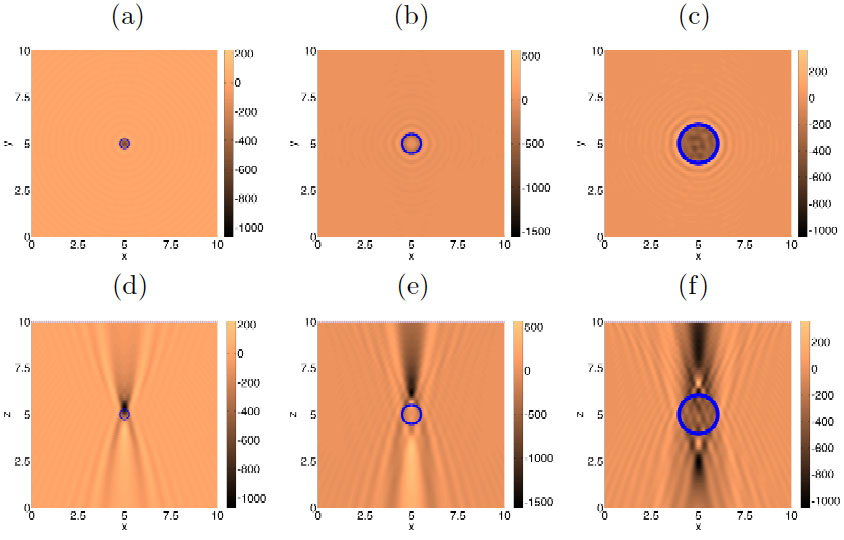
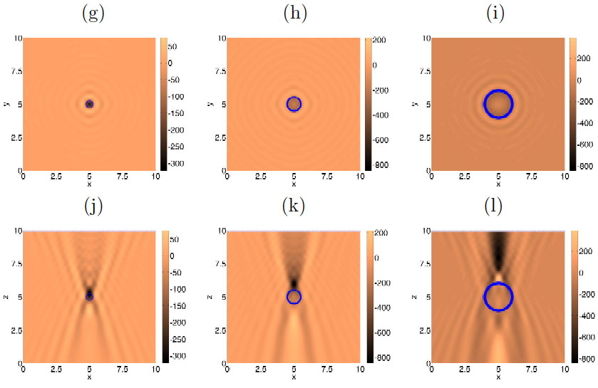
Figure 3: (a)-(c) Slices $z=5$ of the topological derivative evaluated with Eqs. (12) and (15)-(18) for spheres of diameter $0.5$ ($0.5$ $\mu$m), $1$ ($1\ \mu$m) and $2$ ($2\ \mu$m), respectively, centered at $(5,5,5)$ when $k_{e}=20.6$, $k_{i}=24.79$ (violet light). (d)-(f) Same for slices $y=5$. (g)-(i) Same as (a)-(c) when $k_{e}=12.56$, $k_{i}=15.12$ (red light). (j)-(l) Same as (d)-(f) when $k_{e}=12.56$, $k_{i}=15.12$. The borderline of the true objects is superimposed.

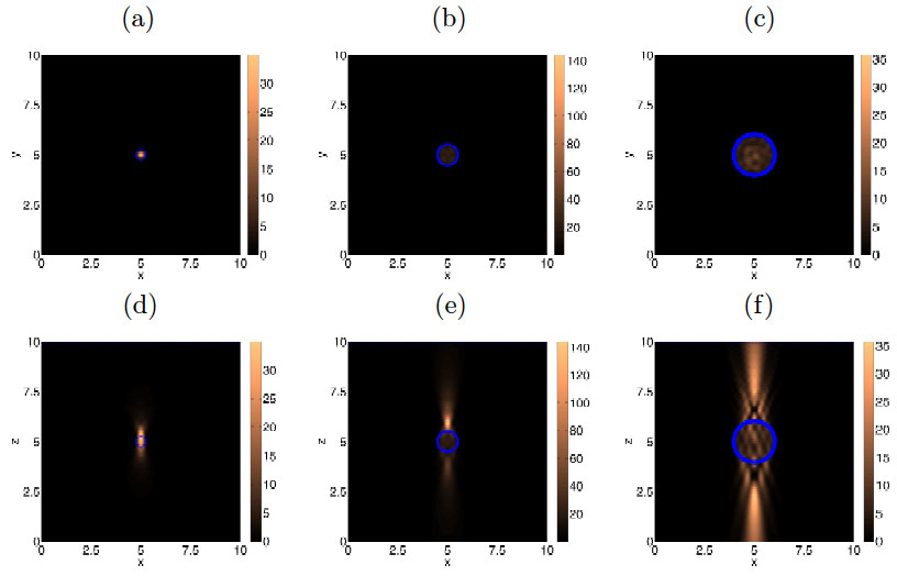
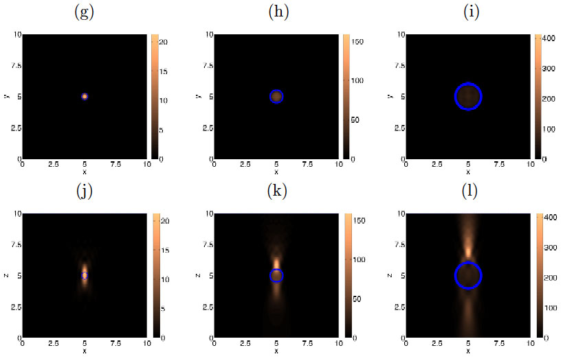
Figure 4: Counterpart of Figure 3, visualizing the topological energy evaluated with Eqs. (19) and (15)-(18), instead of the topological derivative.

For our range of sizes, the topological fields permit to implement a systematic procedure to locate objects employing a single wavelength. A simple strategy to define an initial guess $\Omega_{0}$ for the scatterer sets

$$\Omega_{0}:=\{{\bf x}\in{\mathbb{R}}^{3}\,|\,E_{T}({\bf x},{\mathbb{R}}^{3})\geq C_{0}\}$$ (20)

where $C_{0}$ is a positive constant. Alternatively, we may set

$$\Omega_{0}:=\{{\bf x}\in{\mathbb{R}}^{3}\,|\,D_{T}({\bf x},{\mathbb{R}}^{3})\leq-C_{0}\}.$$ (21)

In both cases, we check that $J({\mathbb{R}}^{3}\setminus\overline{\Omega}_{0})<J({\mathbb{R}}^{3})$. Otherwise, we increase the constant $C_{0}$. Notice that neither the definition of the topological energy (19) nor the analytical expressions for the forward and adjoint fields (15)-(18) depend on $k_{i}$. Therefore, formula (20) provides a first approximation to the objects without knowing their permittivities beforehand. Since the expression for the topological derivative with $\beta=1$ reduces to $D_{T}(\mathbf{x},{\cal R})={\rm Re}[(k_{i}^{2}-k_{e}^{2})E(\mathbf{x})\overline{P}(\mathbf{x})]$, the function ${\rm Re}[E(\mathbf{x})\overline{P}(\mathbf{x})]$ may yield a guess of the objects ignoring the variations of $k_{i}$ too. We usually rely on topological energies to produce first guesses $\Omega_{0}$ since the images are often easier to interpret. Nevertheless, for small enough isolated objects both procedures yield similar estimates and the quality of the predictions improves by iteration, see Sections 5 and 6. As we have commented above, a judicious interpretation of the topological fields may yield better initial guesses of larger objects selecting a range of $z$ between peaks of the topological fields and analyzing the $xy$ sections for that range of $z$. We will discuss this point in more detail in the next section.

If we wish to combine information from data measured for light of different wavelengths, we replace $E_{T}({\bf x},{\mathbb{R}}^{3})$ in definition (20) by the normalized average of the topological energies computed for the two wavelengths at each point (each of them is divided by its global maximum in the region ${\mathcal{R}}_{obs}$ under study):

$$E_{T,a}(\mathbf{x},{\mathbb{R}}^{3})={1\over M_{1}}E_{T,k_{1}}(\mathbf{x},{\mathbb{R}}^{3})+{1\over M_{2}}E_{T,k_{2}}(\mathbf{x},{\mathbb{R}}^{3}),$$

where $M_{\ell}={\rm max}_{\mathbf{x}\in{\cal R}_{obs}}E_{T,k_{\ell}}(\mathbf{x},{\mathbb{R}}^{3})$. A similar normalized average of the topological derivatives may be defined. However, we have not observed a noticeable improvement with these averaging procedures in our numerical tests, though, for specific configurations one wavelength may perform better than the other.

Finally, if we had information from different incident directions, the topological energy fields would be just superimposed, see Section 6.

4 Initial three-dimensional reconstructions

In this section we analyze the performance of topological derivatives and energies when visualizing biological objects of cell structure size using light beams. Figure 5 displays a selection of symmetric, asymmetric, simply connected, multiply connected, convex and non-convex objects that we have considered in our reconstructions. We will see that these fields not only detect the presence of the defects, but are also able to locate them and to distinguish between different configurations and shapes. We can infer the structure of the objects from series of slices in the three space directions.

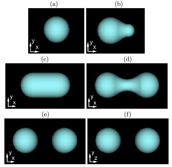
Figure 5: Three-dimensional objects used in the tests. (a) sphere, (b) pear-shaped object, (c) spherocylinder, (d) splitting spherocylinder, (e) two spheres aligned parallel to the screen, (f) two spheres aligned in the beam direction, orthogonal to the screen.

The imaging setting is detailed in Figure 1 and Section 2. After nondimensionalizing, the setting is as follows. We emit one incident wave in the direction $\mathbf{d}=(0,0,1)$, orthogonal to a planar screen located at the plane $z=10$:

$$\Pi_{meas}=[0,10]\times[0,10]\times\{10\}.$$

On this screen we place a uniform grid of detectors, using a step of 0.1 in the $x$ and $y$ directions, located at the points $\{(0.1k,0.1\ell,10)|$ $k,\ell=0,\dots,100\}.$ Typically, objects will be centered about (5,5,5) and we will compute the topological derivative/topological energy in the observation region ${\cal R}_{obs}=[0,10]\times[0,10]\times[0,10],$ where the sample is located. Topological derivatives and energies are computed evaluating formulas (12) and (19), where the forward and adjoint fields are solutions of (15) and (18), respectively. The data $E_{meas}$ are synthetically generated by solving the forward problem (8) for the true defect $\Omega$ using a coupled finite element-boundary element solver for Helmholtz equations inspired in mixed formulations employed in reference [39] for Laplace problems (for further details see also Section 5).

For our numerical experiments we select two representative wavelengths, namely $\lambda^{\rm violet}=405\,{\rm nm}$, $\lambda^{\rm red}=660\,{\rm nm}.$ The corresponding dimensionless parameters are given in Table 2. Notice that the assumption $\beta=1$ implies the disappearance of the gradient term in (12) when computing the topological derivative. In the numerical experiments described here, the exterior and interior wavenumbers are $k_{e}=20.6$ and $k_{i}=24.79$ when using the violet light, or $k_{e}=12.56$ and $k_{i}=15.12$ for the red one. These wavenumbers correspond to typical values of lipid membranes surrounded by water. We have repeated the tests using the intermediate values for $k_{i}$ in Table 2, obtaining similar results. The values for $k_{i}$ are used to generate the synthetic data solving the forward problem and to evaluate topological derivatives. The topological energy only depends on the given data and the value of $k_{e}$, but it does not depend on $k_{i}$.

4.1 Influence of size and position

The structure of the topological derivative (TD) and topological energy (TE) fields changes when the size of the objects vary, as appreciated in Figures 3 and 4. For small objects, with diameters below a micron, the 3D regions where the topological derivative takes large negative values or the topological energy attains its peaks mark the location of the object, giving a reasonable prediction of its size and shape, see panels (a), (d), (g), (j) in Figures 3 and 4. This prediction improves as the size of the object decreases. Moreover, while the offset of the object center becomes negligeable using the largest wavelength (red light), the spurious elongation in the $z$ direction diminishes employing the shortest one (violet). In Section 6 we will see that the prediction of the position, shape and size of the obstacle may be improved by an iterative procedure.

On the contrary, for larger objects, with diameters of a micron and above, the behavior of these fields varies from $xy$ to $xz$ or $yz$ slices. Whereas large negative values of the TD and peaks of the TE reproduce the location, size and shape of $xy$ slices of the object (see panels (c),(i) in Figures 3 and 4), such values concentrate at the edges of the object in $xz$ or $yz$ slices. In particular, panel (f) in Figures 3 and 4 locates the object between peaks of the TD and TE, providing a good guess of its thickness and position relative to the detector screen. This interpretation is clearer for the shorter wavelength in panel (f), than for the larger wavelength in panel (l). A similar situation is observed for a smaller sphere in panels (b),(e),(h),(k) of Figures 3 and 4, with the largest values of the TD and TE located past the object, shifted towards the detector screen, and a weaker peak before the ball.

The described behavior can be related to wavenumber variations observing that we nondimensionlize the problem using a reference object diameter $L=1\,\mu$m. This yields the dimensionless wavenumber values (7) collected in Table 2, that we fix for numerical purposes, while varying the object size. The effective dimensionless wavenumbers are obtained scaling (7) by a factor ${{\cal L}\over L}$, where $\cal L$ is the diameter of the object under study. Their value decreases from panels in the center to panels in the left column of Figures 3-4 by a factor $2$ while it grows by a factor $2$ in the right column. As the size of the object diminishes, we enter the small effective wavenumber regime. Precision improves using the red light, that reduces the wavenumber, enhancing the concentration effect in the object occupied region. Instead, by enlarging the object we enter a high effective wavenumber regime. Resolution improves employing the violet light, which increases the wavenumber further, enhancing the concentration at the borders in the axial direction. The transition to this regime is marked by a decrease in the magnitude of the TD and TE, consequence of the splitting of a peak in two.

Assuming impenetrable objects and short wavelengths, the theoretical analysis in Ref. [30] shows that the brightest points in TD/TE reconstructions are due to caustics. For impenetrable obstacles, the caustics appear exclusively on the back (i.e. ‘dark’) side of an obstacle. Our objects being penetrable, caustics may appear both at the back and the front sides of the anomaly. Secondary reflections off the ‘dark’ side of the boundary are possible, which would become more apparent as the size of the object grows. Our numerical simulations show that bright points on the front side become visible as the object size to wavelength ratio increases, and tend to be weaker than those on the back side, see Fig. 3. The threshold size might be characterized by the above mentioned decrease in the magnitude of the TD. Notice that whereas Ref. [30] takes measurements on a sphere around the object, our measurements are made on a screen past the object. This brings about additional factors, such as the distance to the screen and the size of the screen relative to the object, that influence the structure of the topological fields, as we discuss in Section 4.4.

(a)

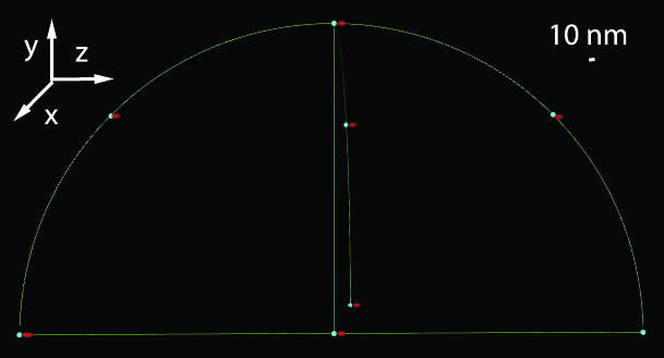
(b)

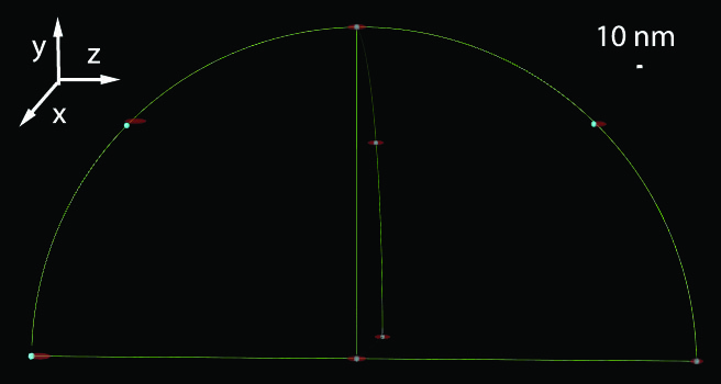
Figure 6: Superimposed reconstructions of isolated balls of diameter $0.01$ ($10$ nm) moving in circles of radius 1 ($1\ \mu$m) about the location $(5,5,5)$: (a) Light of wavelength $405$ nm. (b) Light of wavelength $660$ nm. The true and reconstructed objects are represented in blue and red, respectively.

Let us analyze now the potential of the topological energy to locate the same defect at different positions. These techniques could be employed to track the trajectories of nanoparticles, as evidenced by reconstructions with nanometer scale precision. Figure 6 compares the predicted and true objects, for isolated balls of diameter $0.01$ ($10$ nm) placed at different locations. Using the negative peaks of the TD defined by formula (21) with $C_{0}=-0.9\,{\rm min}_{{\bf x}\in\mathcal{R}_{obs}}\,D_{T}({\bf x},{\mathbb{R}}^{3})$ we determine the center of the approximated objects, and the aspect ratio between the diameters in axial and lateral directions. Information about the true size is inferred from the magnitude of the TD and TE fields, that decreases noticeably with size. For $10$ nm objects, the TE takes maximum values of order $10^{-8}$ for the violet light and $10^{-9}$ for the red one. These values increase to $30$ and $20$, respectively, considering objects of $500$ nm diameter. The reconstructed objects are ellipsoids, slightly elongated in the direction $z$. Notice that the violet light produces less elongated guesses, whereas the red light determines position with more precision. For both wavelengths, the offset and the elongation decrease as we approach the screen.

4.2 Shape identification

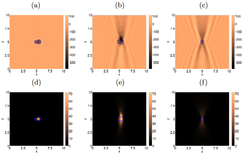
Figure 7: Slices (a) $z=5$, (b) $y=5$ and (c) $x=5$ of the topological derivative when $k_{e}=12.56$ and $k_{i}=15.12$ (red light) for a pear-shaped object of length $1$, and maximum diameter $0.5$. (d)-(f) Same for the topological energy. The blue borderline of the true object is superimposed.

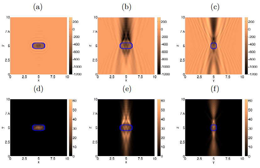
Figure 8: Slices (a) $z=5$, (b) $y=5$ and (c) $x=5$ of the topological derivative when $k_{e}=20.6$ and $k_{i}=24.79$ (violet light) for a spherocylinder of length $2$ and diameter $1$. (d)-(f) Same for the topological energy. The blue borderline of the true object is superimposed.

Figure 9: Slices (a) $z=5$, (b) $y=5$ and (c) $x=5$ of the topological derivative when $k_{e}=20.6$ and $k_{i}=24.79$ (violet light) for a splitting spherocylinder of length $2$ and maximum diameter $1$. (d)-(f) Same for the topological energy. The blue borderline of the true object is superimposed.

(a)                                            (b)

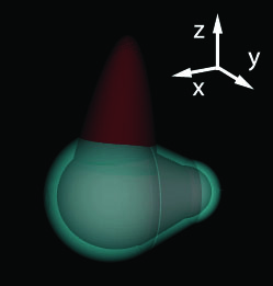
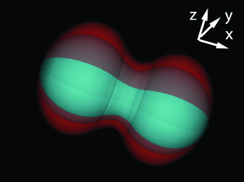
Figure 10: (a) Possible initial reconstruction (red) of the pear-shaped object of length $1$ and maximum diameter $0.5$ using a light beam of wavelength $660$ nm, orthogonal to the detector screen. (b) Possible initial reconstruction (red) of the splitting rod of length $2$ and maximum diameter $1$ using a light beam of wavelength $405$ nm.

Precise information about the shape of the objects can be inferred from $xy$ slices of TD and TE fields. Comparing panels (a),(g) in Figures 3 and 4 to Figure 7(a) and (d) we distinguish the round shape corresponding to a sphere from the pear-like structure depicted in Figure 5(b). Figure 8 represents topological energies and derivatives for the rod-like object shown in Figure 5(c). A narrower central part is appreciated in Figure 9(a) and (d), suggesting a splitting rod, the sand clock shaped object depicted in Figure 5(d). Provided the distance of the object to the screen is approximately known, the slices $z=z_{0}$ of the TD and TE fields allow us to identify the shape of the object, and track changes in its appearance, including asymmetric and non-convex forms.

Besides, the approximate location in the direction $z$ is deduced from the $xz$ and $yz$ slices. Indeed, the prediction of the position is good for the pear-like object using light of wavelength $660$ nm, where the range $z_{0}$ of interest corresponds to the peak of the TE. The prediction of the position obtained in this way improves for smaller objects. On the contrary, for the slightly larger rod and the splitting rod, we may use the $405$ nm light. Then, the range of interest for $z_{0}$ is comprised between the two peaks of the TE. Gathering the information provided by the slices $z=z_{0}$ we propose the reconstructions shown in Figure 10. Panel (a) in this figure uses values $z_{0}$ corresponding to the only peak, whereas panel (b) selects values of $z_{0}$ between the two peaks. More precisely, the reconstruction procedure for a single object is:

• Decide if the effective wavenumber is such that: (a) single objects are located at peaks, or (b) single objects are located between peaks of the TE.

• Determine the relevant range $[z_{1},z_{2}]$ of $z$ to be considered:

  • In case (a), $[z_{1},z_{2}]$ is determined by the lower and upper limits in the $z$ direction of the peak representing the object. Such peak is defined by formula (20), where $C_{0}$ is given by

    $$C_{0}=\alpha_{0}\max_{{\bf x}\in\mathcal{R}_{obs}}E_{T}(\mathbf{x},\mathbb{R}^{3}),\quad 0<\alpha_{0}<1,$$ (22)

    and $\alpha_{0}$ is a value to be calibrated. For example, for the peak-like object we may take $\alpha_{0}=0.5$.

  • In case (b), the range $[z_{1},z_{2}]$ of $z$ is determined by the location of the maxima of the upper and lower peaks.

• For $z_{0}\in[z_{1},z_{2}]$, study the slices $z=z_{0}$ of the topological fields. The rings about the region where the TD takes the largest negative values mark its border. The $z=z_{0}$ slice of the object may be estimated from

  $$\left\{\mathbf{x}=(x,y,z_{0})\big{|}\,D_{T}(\mathbf{x},\mathbb{R}^{3})<-C_{z_{0}}\right\},$$ (23)

  where $C_{z_{0}}=-\alpha_{0}\min_{{\bf x}\in{\cal R}_{obs}\cap\{z=z_{0}\}}D_{T}({\bf x},\mathbb{R}^{3})$.

The three-dimensional images in Figure 10 are VRML (virtual reality modeling language) representations of simple surfaces approximating the reconstructed objects.

4.3 Multiple objects

Standard vision does not detect objects placed behind other objects along the visual line. Moreover, it sometimes identifies objects close to each other as if they were just a single object. On the contrary, our method allows us to distinguish scatterers that would in principle be hidden by previous obstacles in the direction of the incident light; and it is also able to distinguish between multiple defects that are very close.

To illustrate the ability of our method to distinguish objects placed along the same incident direction, Figure 11 analyzes two identical spheres placed along the $z$ axis, as in Figure 5(f). They can be identified with both the $405$ nm and $660$ nm lights. Indeed, unlike the single ball considered in panels (c) and (f) of Figures 3 and 4, the hollow $xy$ slices between the two peaks indicate the presence of two objects placed at the peaks, being the object situated closer to the detector screen the most prominent.

Additional tests show that close objects are distinguishable. Figure 12 represents two spheres located on the plane $z=5$, along the $y$ axis. They are perfectly identified with both wavelengths, though the shortest one yields better resolved shapes. In both cases, the intermediate gap is completely evident, without any blurring. Similar results are observed slightly increasing or decreasing the distance between the objects.

Repeating these tests with objects characterized by different values of $k_{i}$, we obtain similar results, except that the objects with higher contrast $k_{e}^{2}-k_{i}^{2}$ are more clearly distinguished. Notice that topological energies are computed without making use of $k_{i}$. When these values are unknown, the topological energies would yield information on the relative magnitudes of $k_{i}$ for different objects that might be improved by gradient methods [6, 7]. For an increasing number of close spheres, objects blur as the distance between the spheres diminishes, specially in the direction of the incident waves. Resolution is similar provided they are well separated. The topological fields used to define first approximations of the objects use analytical formulas, therefore the number of objects does not pose a difficulty at this stage. It may raise the computational cost of later iterative corrections relying on BEM-FEM methods to evaluate forward and adjoint fields, though.

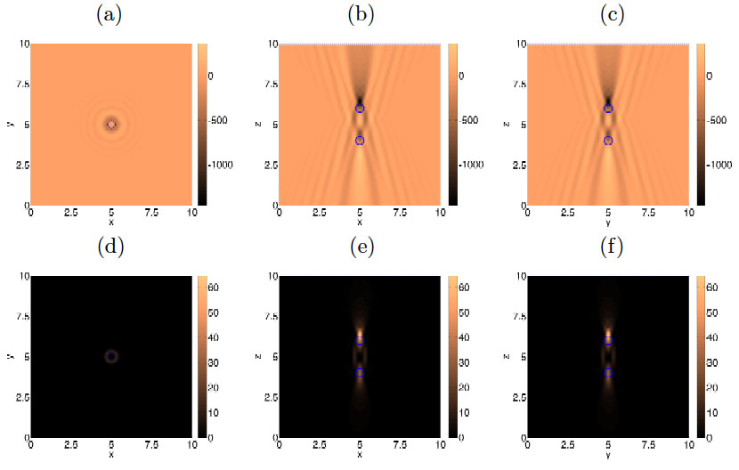
Figure 11: Slices (a) $z=5$, (b) $y=5$ and (c) $x=5$ of the topological derivative when $k_{e}=20.6$ and $k_{i}=24.79$ (violet light). The true objects are two spheres of diameter $0.5$, situated one behind the other along the axis $z$, at distances $4$ and $6$ from the screen. (d) Same for the topological energies. The contour of the true objects is superimposed in (b)-(c) and (e)-(f). No true object is present in (a),(d), though we have superimposed a ghost contour of the balls as reference.

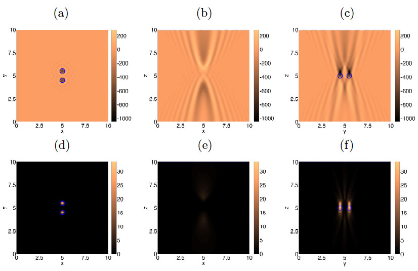
Figure 12: Slices (a) $z=5$, (b) $y=5$ and (c) $x=5$ of the topological derivative when $k_{e}=20.6$ and $k_{i}=24.79$ (violet light). The true objects are two spheres of diameter $0.5$, separated a distance $0.5$ on the plane $z=5$. (d)-(f) Same for the topological energies. The contour of the true objects is superimposed in (a),(c),(d) and (f).

4.4 Influence of the screen size and other parameters

After performing series of numerical experiments varying some of the parameters involved in the imaging setting, we have extracted the following conclusions:

• Fixing the screen size and the distance between detectors, reconstructions worsen when we move the object away from the screen or we displace it left or right noticeably.

• For a fixed screen size, once enough detectors have been placed, increasing the number does not provide significant improvements (replacing the detectors $\{(0.1k,0.1\ell,10)|\,k,\ell=0,\dots,100\}$ by $\{(0.05k,0.05\ell,10)|\,k,\ell=0,\dots,200\}$, for instance).

• For a fixed object size, precision and resolution worsen or improve noticeably by reducing or enlarging the size of the screen. This is specially true for the predicted distance to the screen, in examples such as Fig. 3-4 (d).

We have repeated some of the previous experiments considering the material parameters for nucleus and organelles instead of those for lipid membranes (see Table 2), obtaining similar results. We have also observed that the method is not too sensitive to noise.

5 Postprocessing by iteration

An inspection of the topological energy and derivative of the cost functional (10) when $\Omega=\emptyset$ provides a first guess of the number, location and size of the objects, by means of analytical formulas involving the data, the incident wave and the value of $k_{e}$ for the background medium. If we are only interested in tracking the location or the displacement of objects, or changes of shape in $xy$ sections, this stage may suffice for simple configurations. In general, there is still incertitude about the true number, size, shape and location of objects. Developing methods that are able to improve a first guess $\Omega_{0}$ using only the stored measured data to produce more precise information about the structure of the scatterers $\Omega$ is essential for applications. Here, we introduce a three-dimensional framework to implement topological derivative and energy based iterative schemes overcoming computational difficulties. We set $\beta=1$ and assume $k_{i}$ known, that is often the case when we are just tracking positions and changes of shape. In a more general situation, one can search for both the object $\Omega$ and their material parameters ($\varepsilon_{i}$ and $\mu_{i}$ or equivalently, $\beta$ and $k_{i}$ in this framework). In this case, gradient techniques might yield complementary information about them [6, 7, 8].

5.1 Topological energy based reconstruction algorithm

A simple strategy to define an initial guess $\Omega_{0}$ for the scatterer sets was proposed in Section 3 through formula (20). The positive constant $C_{0}$ is defined by (22), with $0<\alpha_{0}<1$. We have used $\alpha_{0}=0.75$ in our iterative tests.

Once a guess for the objects $\Omega_{0}$ is available, we can modify it evaluating an updated topological energy field. A possible iterative scheme is the following:

• Initialization: Define $\Omega_{0}$ by formula (20).

• Iteration: At each step, a new object $\Omega_{n+1}$ is constructed from $\Omega_{n}$ setting

  $$\Omega_{n+1}:=\{{\bf x}\in\mathbb{R}^{3}\,|\,E_{T}({\bf x},{\mathbb{R}}^{3}\setminus\overline{\Omega}_{n})\geq C_{n+1}\},$$ (24)

  where the topological energy is given by:

  $$E_{T}(\mathbf{x},{\mathbb{R}}^{3}\setminus\overline{\Omega}_{n})=|E_{n}(\mathbf{x})|^{2}|{P}_{n}(\mathbf{x})|^{2},\quad{\bf x}\in\mathbb{R}^{3},$$ (25)

  $E_{n}$ and $P_{n}$ being forward and adjoint fields with object $\Omega_{n}$. This is to say, $E_{n}$ is the solution of the forward problem:

  $$\left\{\begin{array}[]{ll}\Delta E_{n}+k_{e}^{2}E_{n}=0,&\quad\mbox{in $\mathbb{R}^{3}\setminus\overline{\Omega}_{n}$},\\ \Delta E_{n}+k_{i}^{2}E_{n}=0,&\quad\mbox{in $\Omega_{n}$},\\ E_{n}^{-}=E_{n}^{+},&\quad\mbox{on $\partial\Omega_{n}$},\\ \beta\partial_{\mathbf{n}}E_{n}^{-}=\partial_{\mathbf{n}}E_{n}^{+},&\quad\mbox{on $\partial\Omega_{n}$},\\ \displaystyle\lim_{r\to\infty}r\big{(}\partial_{r}(E_{n}-E_{inc})-\imath k_{e}(E_{n}-E_{inc})\big{)}=0,\end{array}\right.$$ (26)

  and $P_{n}$ is the solution of the adjoint problem:

  $$\left\{\begin{array}[]{ll}\Delta P_{n}+{k_{e}^{2}}P_{n}=\sum_{j=1}^{N}(E_{meas,j}-E_{n}(\mathbf{x}_{j}))\delta_{{\mathbf{x}}_{j}}&\quad\mbox{in ${\mathbb{R}}^{3}\setminus\overline{\Omega}_{n}$},\\ \Delta P_{n}+k_{i}^{2}P_{n}=0,&\quad\mbox{in $\Omega_{n}$},\\ P_{n}^{-}=P_{n}^{+},&\quad\mbox{on $\partial\Omega_{n}$},\\ \beta\partial_{\mathbf{n}}P_{n}^{-}=\partial_{\mathbf{n}}P_{n}^{+},&\quad\mbox{on $\partial\Omega_{n}$},\\ \displaystyle\lim_{r\to\infty}r\big{(}\partial_{r}P_{n}+\imath k_{e}P_{n}\big{)}=0.\end{array}\right.$$ (32)

  In practice, we compute the auxiliary field $\overline{P}_{n}$, which is the solution of a problem with the same structure as the forward problem, setting the incident field equal to zero and adding a source $\sum_{j=1}^{N}(\overline{E_{meas,j}-E_{n}(\mathbf{x}_{j})})\delta_{{\mathbf{x}}_{j}}$. Notice that these forward and adjoint fields are defined everywhere, as well as the topological energy.

• Stopping criteria: The iteration should stop if either meas$(\Omega_{n+1}\setminus\Omega_{n})$ is small enough, or $J(\mathbb{R}^{3}\setminus\overline{\Omega}_{n+1})$ is small enough, or the difference of the functional values between consecutive steps is small enough, or the discrepancy principle $\frac{1}{N}\sum_{j=1}^{N}|E_{meas,j}^{\varepsilon}-E_{n+1}(\mathbf{x}_{j})|<\tau\varepsilon$ is satisfied. Here, $\varepsilon$ describes measurement errors and $\tau>1$.

Alternative strategies that only add points to existing guesses forbid removing spurious points, whereas our technique redefines the whole approximation again, allowing us to discard spurious points. For large wavenumbers our method may produce improved guesses of the objects, though convergence is uncertain.

5.2 Topological derivative based reconstruction algorithm

An initial guess $\Omega_{0}$ for the scatterers set was proposed in Section 3 through formula (21). We may take

$$C_{0}=-\alpha_{0}\min_{{\bf x}\in\mathcal{R}_{obs}}D_{T}(\mathbf{x},\mathbb{R}^{3}),$$ (33)

with $0<\alpha_{0}<1$. We have chosen $\alpha_{0}=0.75$ in our iterative tests.

The guess $\Omega_{0}$ can be improved updating the topological derivative field to take into account its presence. The following procedure has been used for two-dimensional tests in acoustics [6]. We adapt it here to our three-dimensional holographic setting.

• Initialization: Define $\Omega_{0}$ by formula (21).

• Iteration: At each step, a new object $\Omega_{n+1}$ is constructed from $\Omega_{n}$ setting

  $$\Omega_{n+1}:=\{{\bf x}\in\Omega_{n}\,|\,D_{T}({\bf x},{\mathbb{R}}^{3}\setminus\overline{\Omega}_{n})<c_{n+1}\}$$

  $$\hskip 28.45274pt\cup\,\{{\bf x}\in\mathbb{R}^{3}\setminus\overline{\Omega}_{n}\,|\,D_{T}({\bf x},{\mathbb{R}}^{3}\setminus\overline{\Omega}_{n})<-C_{n+1}\}.$$ (34)

  For the iterations with the pear-like object discussed in Section 6, we set

  $$C_{1}=-\alpha_{1}\min_{{\bf x}\in\mathcal{R}_{obs}}D_{T}(\mathbf{x},\mathbb{R}^{3}),\quad c_{1}=\beta_{1}\max_{{\bf x}\in\mathcal{R}_{obs}}D_{T}(\mathbf{x},\mathbb{R}^{3}),$$ (35)

  with $\alpha_{1}=1/2$ and $\beta_{1}=1/80.$

  Notice that, at each stage, points where the topological derivative is negative and large are added to existing objects, whereas points where the topological derivative is positive and large are removed from existing objects. The topological derivative is defined for all ${\bf x}\in\mathbb{R}^{3}$ by :

  $$D_{T}(\mathbf{x},{\mathbb{R}}^{3}\setminus\overline{\Omega}_{n})={\rm Re}\Big{[}(k_{i}^{2}-k_{e}^{2})E_{n}(\mathbf{x})\overline{P}_{n}(\mathbf{x})\Big{]},$$ (36)

  $E_{n}$ and $P_{n}$ being forward and adjoint fields with object $\Omega_{n}$, governed by systems (26) and (32) respectively. The positive constants $C_{n+1}$, $c_{n+1}$ in (34) are ultimately chosen to ensure decrease of the cost functional, i.e., $J({\mathbb{R}}^{3}\setminus\overline{\Omega}_{n+1})<J({\mathbb{R}}^{3}\setminus\overline{\Omega}_{n})$. Initially, we may set $C_{n+1}=C_{n}$ and $c_{n+1}=c_{n}$. If the restriction is violated, the values are increased.

• Stopping criteria: The same as for the topological energy based method.

For small enough effective wavenumbers, topological derivative based schemes are expected to produce sequences of approximated objects decreasing the cost functional in view of expansion (11). The effective wavenumbers must be such that the object location in the $z$ direction is marked by one peak about the object location, not two at its edges, as discussed in Section 4.1.

5.3 Implementation

A few technical details about the implementation are in order. The tests presented in Sections 4 and 6 use synthetic data. We place the true objects between the incident wave and the detector screen in the setting described in Sections 1 and 2. Then, we compute the synthetic data solving the forward problem and evaluating the electric field at the detectors. Known the data, we implement the algorithms described in Section 3 and in this section to reconstruct the objects.

Each object $\Omega$ is defined using a signed distance function $f_{d}$, negative inside $\Omega$ and positive outside:

$$\Omega=\{{\mathbf{x}}\in\mathbb{R}^{3}\big{|}\,f_{d}({\mathbf{x}})<0\}.$$ (37)

To solve the forward problem (8) we mesh the object and use a non-symmetric BEM-FEM scheme. More precisely, we generate an unstructured mesh on the object using the open access mesher DistMesh described in Ref. [43]. For the discretization spaces, we use continuous and piecewise $\mathbb{P}1$ finite elements, as well as piecewise constant boundary elements. The boundary integrals entering both the BEM formulation and the BEM-FEM coupling integrals are evaluated following [21]. In particular, boundary integrals are approximated using the Duffy transform, which is a local change of variables that regularizes possible singularities allowing for standard numerical integration (for example, Gauss formulas with six nodes in each direction in our tests). It is well known that the resulting method has order one. We have selected this discretization because it avoids domain truncation or infinite elements. Moreover, it is flexible enough to deal with a wide range of shapes. When $k_{e}$ and $k_{i}$ are constant, faster pure BEM-BEM methods [3] could be used. The BEM-FEM strategy is well suited for more general situations that include the presence of regions with variable parameters inside the objects, or for future combination with gradient strategies to invert also the interior parameters.

The approximated solution of the forward problem for the true objects is evaluated at $101\times 101=10201$ detectors on $[0,10]\times[0,10]\times\{10\}$, on a grid with $101$ values uniformly distributed in each direction:

$$\mathbf{x}_{k,\ell}=(x_{k},y_{\ell},10)=(0.1k,0.1\ell,10),$$ (38)

with $k,\ell=0,...,100$. For each detector, we compute an approximation of the measured wave $E_{meas,k,\ell}\approx E(\mathbf{x}_{k,\ell})$ (where $E$ is the solution of the forward problem (8) for the true defects) using an integral representation of the solution of the scattering problem. More precisely, the solution of the BEM-FEM scheme provides us with approximations of the Cauchy data of the solution of the forward problem, which we can use in Green’s formula and then integrate numerically on each triangle on the boundary (for example, with the barycenter formula in our tests). Further, if necessary, we may compute partial derivatives of the solution just differentiating the integral representation and proceeding as before.

Once an approximation of the measured data is available, we estimate the initial value of the cost functional

$$J({\mathbb{R}}^{3})=\frac{1}{2}\sum_{k,\ell=0}^{100}|E_{inc}(\mathbf{x}_{k,\ell})-E_{meas,k,\ell}|^{2}.$$ (39)

The first topological derivatives and energies are computed using formulas (12) and (19) with forward and adjoint fields given by (15) and (18), respectively. We generate a uniform grid of sampling points $\{\mathbf{y}_{1},\dots,\mathbf{y}_{N_{obs}}\}$ in the region we want to observe, ${\cal R}_{obs}$. In our numerical tests, ${\cal R}_{obs}=[0,10]\times[0,10]\times[0,10]$, and the uniform grid contains $N_{obs}=8\times 10^{6}$ points, obtained by considering 200 points in the $x,y$ and $z$ directions.

To apply the iterative method based on successive computations of topological energies (25) and derivatives (36), we need to define $\Omega_{0}$ (and the subsequent approximations $\Omega_{m}$) by means of a signed distance function which is smooth to be properly meshed with DistMesh. Besides, we want the initial objects $\Omega_{0}$ to approximate identities (20) or (21), whereas the successive corrections $\Omega_{m}$ must approximate the selected definition (24) or (34). Notice that we need to mesh $\Omega_{m}$ to evaluate the cost functional $J({\mathbb{R}}^{3}\setminus\overline{\Omega}_{m})$ corresponding to the proposed reconstruction using formula (10) and to compute adjoint and forward fields in the next iteration. In order to define an adequate signed distance function $f_{d}$ for expression (37) to characterize these domains when meshing with DistMesh, we proceed in several stages:

1. We select a small box $[m_{1},M_{1}]\times[m_{2},M_{2}]\times[m_{3},M_{3}]$ containing $\Omega_{m}$, and we generate a uniform grid of points $\{\mathbf{q}_{1},\dots,\mathbf{q}_{S}\}$, with a small enough step in each direction $d_{q}$ to ensure that a sufficient number of points are inside $\Omega_{m}$ (for example, in our experiments we have taken about $50-110$ auxiliary points inside).

   Notice that this step could be avoided by considering a finer grid $\{\mathbf{y}_{1},\dots,$ $\mathbf{y}_{N_{obs}}\}$ from the beginning. However, if such grid is very fine, then the computational cost in time and memory becomes unnecessarily high. For this reason, we use a somehow coarse grid of the observation region to localize the possible region where the object is located, and once this region has been identified, we consider a finer grid only in that region.

2. We approximate the topological energy in the fine grid $\{\mathbf{q}_{1},\dots,\mathbf{q}_{S}\}$ by linear interpolation of the values in the coarse grid $\{\mathbf{y}_{1},\dots,\mathbf{y}_{N_{obs}}\}$.

   This is faster than using the direct evaluation of the adjoint and forward fields through Green’s formula and, moreover, it smooths the topological fields.

3. We select from $\{\mathbf{q}_{1},\dots,\mathbf{q}_{S}\}$ the points in which the topological energy takes values above thresholds and denote them $\{\widetilde{\mathbf{q}}_{1},\dots,\widetilde{\mathbf{q}}_{S^{\prime}}\}$.

4. We define $\Omega_{m}$ as the smooth union of balls of radius $d$ centered at the points $\{\widetilde{\mathbf{q}}_{1},\dots,\widetilde{\mathbf{q}}_{S^{\prime}}\}$ following the blobby molecule strategy introduced in [2]. More precisely, at any point $\mathbf{x}$ the signed distance function associated to $\Omega_{m}$ is defined as:

   $$f_{d,\Omega_{m}}(\mathbf{x})=\exp(-1)-\sum_{j=1}^{S^{\prime}}\exp(-|\mathbf{x}-\widetilde{\bf q}_{j}|^{2}/(\alpha\,d_{q}^{2})),$$ (40)

   Notice that the radius of each blobbly molecule is $d=d_{q}\sqrt{\alpha}$, $d_{q}$ previously selected at step 1. We may set $\alpha=1$, but it can be increased, for instance to $\alpha=2$; increasing the value of $\alpha$ we obtain a smoother domain, but the size of the domain also increases.

5. Once $\Omega_{m}$ is defined, we generate a mesh using DistMesh and check the mesh quality and the number of nodes. If the values are reasonable, we keep the mesh. Otherwise, when the quality of the mesh is inadequate we modify the points $\{\mathbf{q}_{j}\}$ (that is, $d_{q}$) or the parameter $\alpha$. Besides, if the problem is related to the number of nodes, we modify the diameter of the mesh of $\Omega_{m}$.

6 Shape corrections

Once we have a guess of the number of scatterers, their location and size, we can improve it using the same set of data. Notice that the achievable resolution is limited by the choice of incident directions. Moreover, once enough detectors have been distributed, rising the number does not enhance resolution, though increasing the size of the screen may sharpen it. Let us test how the postprocessing algorithms described in Section 5 may be exploited to refine the first guesses constructed in Section 4.

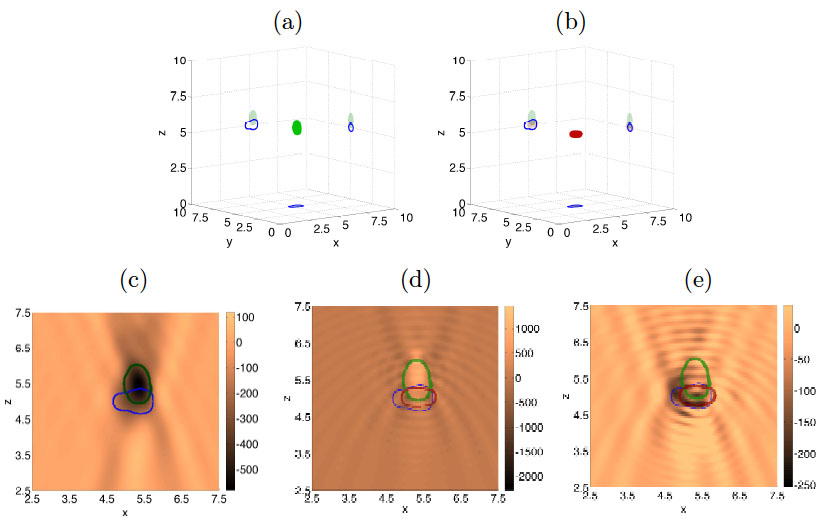
Figure 13: Succesive approximations of the pear-like object in Figure 7 constructed from updated computations of topological derivatives: (a) first guess $\Omega_{0}$, (b) second reconstruction $\Omega_{1}$. Projections on the coordinate planes compare the projection of the true object (blue line) with the projected reconstructions (solid green for $\Omega_{0}$, solid pink for $\Omega_{1}$). Slices $y=5$ of the topological derivative for the first, second and third reconstruction are shown in (c)-(e). The last one suggests adding and removing points to approach the pear-like shape. The blue contour represents the true object, the green contour the first guess, the red contour the second.

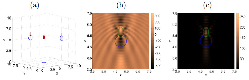
Figure 14: Succesive approximations for the sphere of diameter $1\,\mu$m. (a) Initial guess $\Omega_{0}$. (b)-(c) $y=5$ slices of the topological derivative and the topological energy, respectively, computed with object $\Omega_{0}$ (green contour).

We first revisit the pear-like object considered in Figure 7, illuminated with light of wavelength $660$ nm. Figure 7 displays the initial topological derivatives and energies. We use the topological derivative to define a first approximation through formulas (21) and (33) with $\alpha_{0}=0.75$. Figure 13(a) represents the first reconstruction $\Omega_{0}$ of the object. It is shifted towards the screen and contains points outside the true object. When computing the topological derivative for this first guess $\Omega_{0}$ of the true object, large positive values signal a top region to be removed and large negative values indicate new points to be added, see panel (d) in Figure 13. We create the new object $\Omega_{1}$ using formulas (34)-(35) with $\alpha_{1}=1/2$ and $\beta_{1}=1/80$. Panel (b) represents the new guess after the first iteration. The reconstruction has moved towards the true location, correcting the shape. Computing the topological derivative for this new guess $\Omega_{1}$, we recover the elongated shape, see panel (e).

Next, we revisit the sphere of diameter $1$, located at $(5,5,5)$, illuminated with light of wavelength $660$ nm. The initial topological derivatives and energies are shown in panels (h) and (k) of Figures 3 and 4. We use the topological energy to define a first approximation through formulas (20) and (22) with $\alpha_{0}=0.75$. Figure 14 displays the topological derivatives and topological energies computed after the first iteration. Notice that only the bottom part of the initial object $\Omega_{0}$ remains in the next approximation $\Omega_{1}$, since the topological derivative is large and positive in the rest. Moreover, the topological derivative shows a prominent negative region below, covering the diameter of the true object. Other negative regions outside are an artifact associated to the spurious points included in $\Omega_{0}$. We can propose a new approximation $\Omega_{1}$ using either the peak of the topological energy (24) or the strategy (34) for the topological derivative. The computation of updated topological energies and derivatives in both cases does not yield a clear improvement. Instead, increasing the number of incident directions provides a much sharper reconstruction. In particular, we have analyzed the effect of superimposing the normalized TD and TE fields obtained adding four incident lights forming angles of $45$ degrees with the orthogonal one, in a symmetric way not to bias the information on the object shape. Some results for the ball of diameter $1\,\mu$m are shown in Figure 15. The TE fields seem to be easier to interpret than the TD fields, suggesting consistently the presence of an object about the true location, with accurate $xy$ sections, but slightly elongated in the $z$ direction. Notice that the prediction is better for the red light, as shown by the contours corresponding to a level $0.75\,{\rm max}_{\mathbf{x}\in\mathcal{R}_{obs}}\,E_{T}({\bf x},{\mathbb{R}}^{3})^{1/2}$. We have chosen to plot $E_{T}^{1/2}$ here to better visualize the shape. The TE fields enhance the peaks and reduce intermediate values. This effect is useful to distinguish different objects, but may underestimate points around the peaks belonging to them. Single objects are sometimes more easily reconstructed using $E_{T}^{1/2}$, as it happens in this case. The algorithm that reconstructs objects glueing together 2D sections along a suitable range $[z_{1},z_{2}]$ described in Section 4.2, might produce comparable results, provided we are able to calibrate all the thresholds properly.

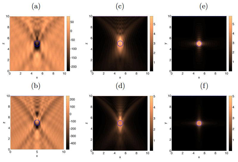
Figure 15: Topological derivatives and topological energies obtained superimposing the fields corresponding to five incident waves for the sphere of diameter $1\,\mu$m, one orthogonal to the detector screen and four symmetric ones forming angles of amplitude $\pi/4$ with it. (a)-(b) Averaged topological derivatives at $y=5$ for the red and violet lights, respectively. (c)-(d) Averaged square root of the topological energies at $y=5$ for the red and violet lights, respectively. (e)-(f) Same at planes $z=5$. The blue contour of the true object is superimposed.

7 Conclusions and future work

In microsystems such as cells, relevant structures span over a wide range of finer scales, down to a few nanometers. Non-invasive techniques which enable imaging biological samples over a range of spatial and temporal scales are of great value. We have considered an imaging microsystem based on recording scattered light of single wavelengths on a screen. This system displays a large range of effective wavenumbers depending on the geometry of the objects under study. Moreover, the possibility of employing several incident directions is restricted. Blending several wavelengths does not yield significative improvements either. We have shown that analytical formulas for the topological derivatives and energies of associated cost functionals provide good guesses of a variety of three-dimensional configurations, based on the knowledge on the electric field at the detectors, the incident light field and the background permittivity.

Using one incident wave, impinging orthogonally to the detector screen, we have discovered that topological methods allow us to locate isolated objects with diameters down to $10$ nm and trace their position with nanometer precision. Lateral sections of the topological fields, orthogonal to the incidence direction, reproduce the form and size of the true objects for a variety of sizes and geometries. This would allow us to track shape changes with time. Asymmetric, non-convex and multiple contours are distinguishable. Furthermore, multiple scatterers distributed along axial and lateral directions are clearly identified. On the other hand, axial information on single objects, in the direction of the incident beam, must be interpreted taking into account the effective wavenumber, relative to the employed wavelength, and the object size. Indeed, for sizes above a micron, objects can be approximated connecting predictions of two-dimensional sections along an axial range determined by two peaks in the topological fields, before and past the object. For larger wavelengths, or smaller sizes, the two-dimensional sections of interest lie along a peak of the topological field, usually with an offset towards the detector screen. This offset decreases as the size of the object diminishes. Besides, the elongation of the peak in the axial direction shrinks as the wavelength decreases, though the position may be more accurately described increasing the wavelength.

Assuming the permittivities of the objects known, we have tested different iterative procedures to refine initial reconstructions keeping the same measured data, while improving the shape and position of the reconstructions. For small enough objects, topological derivative based iterations are suitable to approximate their size and shape in a converging way. In general, topological energies are usually more effective than topological derivatives to propose initial guesses because they are often easier to interpret in presence of oscillations, and the predicted position tends to be more accurate. Moreover, additional iterations based on topological energies may correct the offset. These refined guesses can also serve as starting point of alternative imaging algorithms that employ shape optimization or level set dynamics to fit object contours, or gradient strategies to reconstruct unknown permittivity profiles.

For specific choices of object sizes, depending on the distance to the screen, the area covered by detectors and the distance between them, the first reconstruction provided by the topological fields may be acceptable. Modifying these parameters to adapt them to the spatial scales of interest is another way of focusing the produced image. Here, we have analyzed the effect of incorporating a limited number of incident waves, showing that this procedure largely improves the predictions of position and size.

Summarizing, this work demonstrates the potential of topological techniques in holographic microscopy. However, our imaging setting assumes that we are able to measure the full wave field at the screen detectors. The data actually measured in holography are slightly different. Both data types might be related as mentioned in the introduction, provided a way to estimate background fields is devised. Nevertheless, further work is required to be able to apply these reconstruction procedures in holographic microscopes. Proposing a deterministic (no or minimal human input needed) algorithm for turning topological fields into 3D models of objects would be of great value. Our methods might be useful in other electromagnetic imaging problems, such as microwave imaging, where electric fields are recorded and information from more sources is available.

Acknowledgements. A. Carpio thanks M.P. Brenner for hospitality while visiting Harvard University financed by a Caja Madrid Mobility grant. T.G. Dimiduk and A. Carpio thank the Kavli Institute Seminars at Harvard for the interdisciplinary communication environment that initiated this work. T.G. Dimiduk acknowledges the support of a National Science Foundation (NSF) Graduate Research Fellowship. This research was also supported by MINECO grants No. FIS2011-28838-C02-02 (AC), No. MTM2014-56948-C2-1-P (AC, MLR), No. TRA2013-45808-R (MLR), No. MTM2013-43671-P (VS). Part of the computations of this work were performed in EOLO, the HPC of Climate Change of the Moncloa International Campus of Excellence, funded by MECD and MICINN.

References

- [1] D. Baddeley, C. Batram, Y. Weiland, C. Cremer, U.J. Birk, Nanostructure analysis using spatially modulated illumination microscopy, Nature protocols, 2 (2003), pp. 2640-2646.
- [2] J.F. Blinn, A generalization of algebraic surface drawing, ACM Transactions on graphics, 1 (1982), pp. 235-256.
- [3] O.P. Bruno, L.A. Kunyansky, A fast high-order algorithm for the solution of surface scattering problems: basic implementation tests and applications, J. Comput. Phys. 169 (2001) 80-110.
- [4] M. Born, E. Wolf, Principles of Optics, Cambridge University Press, 1997.
- [5] A. Carpio, M. L. Rapún, Topological derivatives for shape reconstruction, In Inverse problems and imaging, Lect. Not. Math., 1943, pp. 85-133, Springer, Berlin, 2008.
- [6] A. Carpio, M.L. Rapún, Solving inverse inhomogeneous problems by topological derivative methods, Inv. Probl., 24 (2008), 045014.
- [7] A. Carpio, M.L. Rapún, An iterative method for parameter identication and shape reconstruction, Inverse Probl. Sci. Eng. 18 (2010), pp. 35-50.
- [8] A. Carpio, M.L. Rapún, Hybrid topological derivative and gradient-based methods for electrical impedance tomography, Inv. Probl., 28 (2012), 095010.
- [9] I. Catapano, L. Crocco, M. D Urso,T. Isernia, 3D microwave imaging via preliminary support reconstruction: testing on the Fresnel 2008 database, Inv. Probl. 25 (2009), 024002.
- [10] F. Caubet, M. Godoy, C. Conca, On the detection of several obstacles in 2D Stokes flow: topological sensitivity and combination with shape derivatives, Inverse Probl. Imaging, 10 (2016), 327-367.
- [11] P.C. Chaumet, K. Belkebir, Three-dimensional reconstruction from real data using a conjugate gradient-coupled dipole method, Inv. Probl., 25 (2009), 024003
- [12] F.C. Cheong, B.J. Krishnatreya, D.G Grier, Strategies for three-dimensional particle tracking with holographic video microscopy, Optics Express 18 (2010), pp. 13563-13573.
- [13] D. Colton, The inverse scattering problem for time–harmonic acoustic waves, SIAM Rev., 26 (1894), pp. 323-350.
- [14] D. Colton, R. Kress R, Inverse acoustic and electromagnetic scattering theory, Springer, Berlin, 1992.
- [15] T.G. Dimiduk, R.W. Perry, J. Fung, V.N. Manoharan, Random-subset fitting of digital holograms for fast three-dimensional particle tracking, Appl. Opt. 53 (2014), pp. G177-G183.
- [16] L. Dixon, F.C. Cheong, D.G. Grier, Holographic deconvolution microscopy for high-resolution particle tracking, Optics Express 19 (2011), pp. 16410-16417.
- [17] N. Dominguez, V. Gibiat, Non-destructive imaging using the time domain topological energy method, Ultrasonics, 50 (2010), pp. 367-372.
- [18] O. Dorn, D. Lesselier, Level set methods for inverse scattering, Inv. Probl., 22 (2006), pp. R67-R131.
- [19] O. Dorn, D. Lesselier, Level set methods for inverse scattering-some recent developments, Inv. Probl., 25 (2009), 125001.
- [20] A. Egner, S. Jakobs, S.W. Hell, Fast 100-nm resolution three-dimensional microscope reveals structural plasticity of mitochondria in live yeast, Proc. Nat. Acad. Sc, 99 (2002), pp. 3370-3375.
- [21] S. Erichsen, S.A. Sauter, Efficient automatic quadrature in 3-d Galerkin BEM, Comput. Methods Appl. Mech. Eng., 157 (1998), pp. 215-224.
- [22] C. Eyraud, A. Litman, A. Hérique, W. Kofman, Microwave imaging from experimental data within a Bayesian framework with realistic random noise, Inv. Probl., 25 (2009), 024005.
- [23] G.R. Feijoo, A new method in inverse scattering based on the topological derivative, Inv. Probl., 20 (2004), pp. 1819-1840
- [24] P. Ferraro, S. Grilli, D. Alfieri, S. Nicola, A. De; Finizio, G. Pierattini, B. Javidi, G. Coppola, V. Striano, Extended focused image in microscopy by digital holography, Opt. Expr., 13 (2005), pp. 6738-6749.
- [25] J.F. Funes, J.M. Perales, M.L. Rapún, J.M. Vega, Defect detection from multi–frequency limited data via topological sensitivity, J. Math. Imag. Vis. 55 (2016), pp. 19-35.
- [26] J. Fung, R. W. Perry, T. G. Dimiduk, V. N. Manoharan, Imaging multiple colloidal particles by fitting electromagnetic scattering solutions to digital holograms, J. Quant. Spectroscopy and Radiative Transfer 113 (2012), pp. 212-219.
- [27] J. Ge, D.K. Wood, D.M. Weingeist, S. Prasongtanakij, P. Navasumrit, M. Ruchirawat, B.P. Engelward, Standard fluorescent imaging of live cells is highly genotoxic, Cytometry Part A, 83A (2013), pp. 552-560.
- [28] B.B. Guzina, M. Bonnet M, Small-inclusion asymptotic of misfit functionals for inverse problems in acoustics, Inv. Probl., 22 (2006), 1761-1785
- [29] B.B. Guzina, I. Chikichev, From imaging to material identification: A generalized concept of topological sensitivity, J. Mech. Phys. Sol., 55 (2007), pp. 245-279
- [30] B. Guzina, F. Pouhramadian, Why the high-frequency inverse scattering by topological sensitivity may work, Proc. R. Soc. A., 471 (2015), 2179.
- [31] G. Indebetouw, P. Klysubun, A posteriori processing of spatiotemporal digital microholograms, J. Opt. Soc. Am. A, 18 (2001), pp 326-331.
- [32] D. M. Kaz, R. McGorty, M. Mani, M. P. Brenner, and V.N. Manoharan, Physical ageing of the contact line on colloidal particles at liquid interfaces, Nature Materials, 11 (2011), pp. 138-142.
- [33] Y. Kuznetsova, A. Neumann, S.R.Brueck, Imaging interferometric microscopy-approaching the linear systems limits of optical resolution, Opt. Expr., 15 (2007), pp. 6651-6663.
- [34] T. Latychevskaia, H.W. Fink, Resolution enhancement in digital holography by self-extrapolation of holograms, Opt. Expr., 21 (2013), pp. 7726-7733.
- [35] S.H. Lee, Y. Roichman, G.R. Yi, S.H. Kim, S.M. Yang, A. van Blaaderen, P. van Oostrum, D. G. Grier, Characterizing and tracking single colloidal particles with video holographic microscopy, Opt. Expr. 15 (2007), pp. 18275-18282.
- [36] M. Li, A. Abubakar, P.M. van den Berg, Application of the multiplicative regularized contrast source inversion method on 3D experimental Fresnel data, Inverse Problems 25 (2009) 024006.
- [37] Electromagnetic fields in biological systems, J.C. Lin Ed., CRC press, 2011
- [38] P. Marquet, B. Rappaz, P. J. Magistretti, E. Cuche, Y. Emery, T. Colomb, C. Depeursinge, Digital holographic microscopy: a noninvasive contrast imaging technique allowing quantitative visualization of living cells with subwavelength axial accuracy, Opt. Lett., 30 (2005), pp. 468-478.
- [39] S. Meddahi, F.J. Sayas, V. Selgas, Non-symmetric coupling of BEM and mixed FEM on polyhedral interfaces, Mathematics of Computation, 80 (2011), pp. 43-68.
- [40] W.K. Park, Multifrequency topological derivative for approximate shape acquisition of curve–like thin electromagnetic inhomogeneities, J. Math. Anal. Appl., 404 (2013), pp. 501-518.
- [41] Handbook of Biological Confocal Microscopy, J.B. Pawley JB (Ed.), Springer (2006).
- [42] R. W. Perry, G. Meng, T. G. Dimiduk, J. Fung, V. N. Manoharan, Real-space studies of the structure and dynamics of self-assembled colloidal clusters, Faraday Discussions, 159 (2012), pp. 211-234.
- [43] P.O. Persson, G. Strang, A simple mesh generator in MATLAB, SIAM Review, 46 (2004), pp. 329-345.
- [44] M. Pluta, Advanced Light Microscopy, Vol. 2, Elsevier, New York, 1988.
- [45] J. Reymann, D. Baddeley, M. Gunkel, P. Lemmer, W. Stadter, T. Jegou, K. Rippe, C. Cremer, U. Birk, High-precision structural analysis of subnuclear complexes in fixed and live cells via spatially modulated illumination (SMI) microscopy, Chromosome research: an international journal on the molecular, supramolecular and evolutionary aspects of chromosome biology, 16 (2008), pp. 367-282.
- [46] U. Schnars, W.P.O. Jüptner, Digital recording and numerical reconstruction of holograms, Meas. Sci. Technol., 13 (2002), pp. R85-R101.
- [47] J. Sheng, E. Malkiel, J. Katz, J. Adolf, R. Belas, Digital holographic microscopy reveals prey-induced changes in swimming behavior of predatory dinoflagellates, Proc. Nat. Acad. Sc. , 10(2007), pp. 17512-17517.
- [48] J. Sokowloski, A. Zochowski, On the topological derivative in shape optimization, SIAM J. Control Optim., 37 (1999), pp.1251–1272.
- [49] P.W.M. Tsang, K. Cheung, T. Kim, Y. Kim, T. Poon, Fast reconstruction of sectional images in digital holography, Opt. Lett. (2011), pp. 2650-2652.
- [50] T. Vincent, Introduction to Holography, CRC Press, 2012
- [51] A. Wang, T.G. Dimiduk, J. Fung, S. Razavi, I. Kretzschmar, K. Chaudhary, V.N. Manoharan, Using the discrete dipole approximation and holographic microscopy to measure rotational dynamics of non-spherical colloidal particles, J. Quant. Spectroscopy and Radiative Transfer, 146 (2014), pp. 499-509.
- [52] C. Yu, M. Yuan, Q.H. Liu, Reconstruction of 3D objects from multi-frequency experimental data with a fast DBIM-BCGS method, Inv. Probl., 25 (2009), 024007.
- [53] J. De Zaeytijd, A. Franchois, Three-dimensional quantitative microwave imaging from measured data with multiplicative smoothing and value picking regularization, Inv. Probl., 25 (2009), 024004.
- [54] X. Zhang, E. Lam, T.C. Poon, Reconstruction of sectional images in holography using inverse imaging, Opt. Expr., 16 (2008), pp. 17215-17226.