Emergent eddy saturation from an energy constrained eddy parameterisation

Abstract

The large-scale features of the global ocean circulation and the sensitivity of these features with respect to forcing changes are critically dependent upon the influence of the mesoscale eddy field. One such feature, observed in numerical simulations whereby the mesoscale eddy field is at least partially resolved, is the phenomenon of eddy saturation, where the time-mean circumpolar transport of the Antarctic Circumpolar Current displays relative insensitivity to wind forcing changes. Coarse-resolution models employing the Gent–McWilliams parameterisation with a constant Gent–McWilliams coefficient seem unable to reproduce this phenomenon. In this article, an idealised model for a wind-forced, zonally symmetric flow in a channel is used to investigate the sensitivity of the circumpolar transport to changes in wind forcing under different eddy closures. It is shown that, when coupled to a simple parameterised eddy energy budget, the Gent–McWilliams coefficient of the form described in Marshall et al. (2012) [A framework for parameterizing eddy potential vorticity fluxes, J. Phys. Oceanogr., vol. 42, 539–557], which includes a linear eddy energy dependence, produces eddy saturation as an emergent property.

1 Introduction

Studies of the response of the large-scale ocean circulation to changing forcing scenarios in numerical ocean models, and its resulting climatology, require long time integrations that are prohibitively expensive even at mesoscale eddy permitting resolutions. Since this is expected to remain the case for the foreseeable future, an ongoing challenge in numerical ocean modelling is the representation of the unresolved mesoscale eddy field in coarse resolution models. A particularly successful scheme that is employed is the Gent–McWilliams closure (Gent and McWilliams, 1990; Gent et al., 1995, hereafter GM), which parameterises mesoscale eddies via the introduction of a non-divergent eddy transport velocity. The eddy transport velocity can be interpreted as arising from the difference between the Eulerian average of the velocity at fixed height and the thickness-weighted average of the velocity at fixed density (McDougall and McIntosh, 2001), and modifies the advective transport of tracer quantities. By definition, the non-divergent eddy transport velocity conserves all moments of the advected quantities, and is thereby adiabatic. The property of adiabatic stirring is particularly attractive, being shown to remove spurious heating and cooling in the deep ocean, such as that associated with the Deacon cell in the Southern Ocean (Danabasoglu et al., 1994).

To this point, studying the modelled oceanic response to changing atmospheric forcing in conjunction with the GM parameterisation is of particular importance for emergent climatologies under different forcing scenarios. Two important large-scale Southern Ocean phenomena are of particular interest in this regard. The first is “eddy saturation”, originally discussed in Straub (1993) from an argument based on critical stability, and here to be understood as the relative insensitivity of the time-mean circumpolar transport with respect to wind forcing changes. The other is “eddy compensation”, here to be understood as the reduced sensitivity of the residual meridional overturning circulation with wind forcing changes (e.g., Meredith et al., 2012; Viebahn and Eden, 2012; Munday et al., 2013), which has consequences for the meridional transport of important tracers such as heat, salt and carbon. This article focuses on eddy saturation.

As argued by Straub (1993), if fluid interaction with topography is the main sink for momentum input by wind stress, and consequently the zonal abyssal flow is weak, then thermal wind shear is the dominant contribution to circumpolar transport. Thus circumpolar transport is intimately linked to isopycnal slope, with the slope steepness limited by baroclinic instability. Eddy saturation arises through a balance between steepening of isopycnals by wind stress, and flattening of isopycnals by the presence of the mesoscale eddy field. The reduction in circumpolar transport sensitivity with varying wind stress has been observed in a variety of numerical models that at least partially resolves a mesoscale eddy field (e.g., Hallberg and Gnanadesikan, 2006; Hogg and Blundell, 2006; Hogg et al., 2008; Farneti and Delworth, 2010). In Munday et al. (2013), an eddy permitting one-sixth degree model of a 20 degree wide ocean sector was integrated with varying wind forcings. This eddy permitting model, employing a very small value of the GM coefficient, showed near complete eddy saturation. By contrast, in lower resolution half degree and two degree variants of the same model, where larger values of the GM coefficient were utilised, the resulting time-mean circumpolar transport displayed significant sensitivity with respect to the wind forcing. Hogg and Munday (2014) found that although the value of the time-mean circumpolar transport was affected by the domain geometry, the relative insensitivity with changing wind stress at eddy permitting resolution was robust.

Thus it has been found that the GM scheme with spatially and temporally constant GM coefficient is unable to represent eddy saturation. With increased wind forcing, a more vigourous eddy field is to be expected. Since the GM coefficient in some sense specifies the intensity and efficiency of the parameterised eddy field, it is expected that a positive correlation between the strength of wind forcing and the magnitude GM coefficient is minimally required for emergent eddy saturation. Various proposals already exist with a non-constant GM coefficient. Visbeck et al. (1997), using linear stability arguments, proposes a GM coefficient which depends upon the stratification profile, as well as a mixing length. In Ferreira et al. (2005) the eddy-mean-flow interaction in a global ocean model is determined via an optimisation procedure, yielding diagnosed values for the GM coefficient. This is used to infer a GM coefficient which depends on the vertical stratification, and has subsequently been incorporated into a number of ocean general circulation models (e.g., Danabasoglu and Marshall, 2007; Gent and Danabasoglu, 2011). The simulations described in Gent and Danabasoglu (2011) do show some eddy compensation, as a consequence of the dependence of the GM coefficient on Southern Ocean stratification. However, as discussed in Munday et al. (2013), this mechanism precludes the model from achieving full eddy saturation. A case where the GM coefficient is varied manually with changing wind stress has also been investigated (Fyfe et al., 2007). Through the consideration of the eddy kinetic energy budget, Cessi (2008) proposes a mixing length based eddy parameterisation, with a GM coefficient depending on the ocean state and also explicitly depending on the strength of the bottom drag. An approach also based upon consideration of the eddy kinetic energy budget is discussed in Eden and Greatbatch (2008), also employing a mixing length argument but utilising a local parameterised eddy kinetic energy budget to inform the magnitude and spatial structure of the resulting GM coefficient.

In Marshall et al. (2012) a geometric interpretation of the eddy-mean-flow interaction for the quasi-geostrophic equations was derived. A horizontally down-gradient closure for the horizontal eddy buoyancy fluxes leads to a GM coefficient of the form

$$\kappa=\alpha E\frac{N}{M^{2}},$$ (1)

where $E$ is the total (kinetic plus potential) eddy energy, and $N/M^{2}=T$ is an Eady time-scale which depends on the mean stratification, with $N^{2}=-(g/\rho_{0})\partial\overline{\rho}/\partial z$ and $M^{2}=(g/\rho_{0})\left|\nabla_{H}\overline{\rho}\right|$, where $g$ is the gravitational acceleration, $\rho_{0}$ is a reference density, $\overline{\rho}$ is the mean density, and $\nabla_{H}\overline{\rho}$ is its horizontal gradient. A crucial point is that, if the eddy energy is known, there are no undetermined dimensional parameters; the only freedom is to specify the non-dimensional geometric parameter $\alpha$ of magnitude less than or equal to one.

This article assesses the ability of the Marshall et al. (2012) for of the GM coefficient in producing emergent eddy saturation, via numerical calculations in an idealised, zonally averaged, two-dimensional ocean channel model. The idealised numerical model is motivated by the physical model discussed in Marshall et al. (submitted). The performance is compared against a number of alternative approaches, including approaches based upon mixing length arguments, and based upon the Visbeck et al. (1997) proposal. Since the Marshall et al. (2012) variant requires information about the eddy energy, the evolution of the mean state is coupled to a simple prognostic equation for the parameterised domain integrated eddy energy (cf. the local budget for the eddy kinetic energy in Eden and Greatbatch 2008).

A form similar to (1) also appears in Jansen et al. (2015) — implied by their equations (9) and (11) — but with the eddy kinetic energy in place of the full eddy energy, and motivated by the inverse energy cascade being controlled by the rate of eddy energy generation through baroclinic instability as per Larichev and Held (1995). However the form derived in Marshall et al. (2012) provides an explicit upper bound on the relevant geometric parameter $\alpha$. Hence no other dimensional scaling is possible provided the geometric parameter $\alpha$ is bounded away from zero. Moreover here the eddy energy is determined prognostically via the solution of a dynamical equation which is coupled to the equations for the mean state.

The paper proceeds as follows. In §2 the GM scheme and the Marshall et al. (2012) parameterisation variant are revisited, focusing in particular on the energetics of the problem, and providing physical and mathematical arguments as to why the Marshall et al. (2012) variant may be expected to have skill in producing emergent eddy saturation. §3 contains the details of the idealised numerical model and details of the other parameterisation variants considered in this work. The actual implementation of the parameterisation variants and their results are presented in §4 for a case where the GM coefficient is assumed to be constant over the domain, and in §5 for a case where the GM coefficient is spatially varying, focusing on the case where a spatial structure depending upon the vertical stratification is enforced. The paper concludes in §6, where the results are discussed, and a recipe for implementation in a general global circulation models is proposed.

2 Gent–McWilliams and energetic constraints

2.1 The Gent–McWilliams scheme and the energetic consequences

The GM scheme parameterises the effects of baroclinic eddies via the introduction of an adiabatic stirring of the mean density, acting to decrease the available potential energy of the system (e.g., Gent and McWilliams, 1990). Limiting consideration to the Boussinesq case, the mean density equation, zonally averaged at constant density (Andrews, 1983; McDougall and McIntosh, 2001; Young, 2012), is

$$\frac{\partial{\overline{\rho}}^{\rho}}{\partial t}+\frac{\partial\left(\hat{v}~{}{\overline{\rho}}^{\rho}\right)}{\partial y}+\frac{\partial\left(\hat{w}~{}{\overline{\rho}}^{\rho}\right)}{\partial z}=0,$$ (2)

where $\overline{\left(\ldots\right)}^{\rho}$ indicates a zonal average at constant density, with

$$\hat{v}=\overline{v\left(\frac{\partial\rho}{\partial z}\right)^{-1}}^{\rho}\frac{\partial{\overline{\rho}}^{\rho}}{\partial z}$$ (3)

the thickness-weight averaged meridional velocity at constant density, and $\hat{w}$ defined such that

$$\frac{\partial\hat{v}}{\partial y}+\frac{\partial\hat{w}}{\partial z}=0.$$ (4)

Following McDougall and McIntosh (2001),

$$\hat{\boldsymbol{u}}=\left(\begin{array}[]{c}0\\ \hat{v}\\ \hat{w}\end{array}\right)=\left(\begin{array}[]{c}0\\ \overline{v}^{z}\\ \overline{w}^{z}\end{array}\right)+\left(\begin{array}[]{c}0\\ v^{*}\\ w^{*}\end{array}\right)=\overline{\boldsymbol{u}}^{z}+\boldsymbol{u}^{*},$$ (5)

where $\overline{\boldsymbol{u}}^{z}$ is the velocity zonally averaged at constant height, and $\boldsymbol{u}^{*}$ is the eddy transport velocity, with

$$\frac{\partial\overline{v}^{z}}{\partial y}+\frac{\partial\overline{w}^{z}}{\partial z}=\frac{\partial v^{*}}{\partial y}+\frac{\partial w^{*}}{\partial z}=0.$$ (6)

The GM scheme then takes the form

$$\boldsymbol{u}^{*}=\nabla\times\left(\begin{array}[]{c}-\kappa s\\ 0\\ 0\end{array}\right)=\left(\begin{array}[]{c}0\\ -\partial\left(\kappa s\right)/\partial z\\ \partial\left(\kappa s\right)/\partial y\end{array}\right),$$ (7)

where $\kappa$ is the GM eddy transfer coefficient, and $s$ is the slope of the mean density surfaces

$$s=-\left(\frac{\partial\overline{\rho}^{\rho}}{\partial y}\right)\left(\frac{\partial\overline{\rho}^{\rho}}{\partial z}\right)^{-1}.$$ (8)

The energetic consequences of the GM scheme are as follows. Consider the zonally averaged hydrostatic Boussinesq equations in the form

$$\frac{\partial\overline{u}^{z}}{\partial t}+\overline{v}^{z}\frac{\partial\overline{u}^{z}}{\partial y}+\overline{w}^{z}\frac{\partial\overline{u}^{z}}{\partial z}-f\overline{v}^{z} =\overline{F}^{z}-\overline{D}^{z},$$ (9a)

$$\frac{\partial\overline{v}^{z}}{\partial t}+\overline{v}^{z}\frac{\partial\overline{v}^{z}}{\partial y}+\overline{w}^{z}\frac{\partial\overline{v}^{z}}{\partial z}+f\overline{u}^{z} =-\frac{1}{\rho_{0}}\frac{\partial\overline{p}^{z}}{\partial y},$$ (9b)

$$0 =-\frac{1}{\rho_{0}}\frac{\partial\overline{p}^{z}}{\partial z}-\frac{g\overline{\rho}^{\rho}}{\rho_{0}}.$$ (9c)

Here contributions from Reynolds stresses are neglected, it is assumed that all significant forcing $\overline{F}^{z}$ and dissipation $\overline{D}^{z}$ occurs in the zonal mean momentum equation, and $\overline{\rho}^{\rho}$ is used in place of $\overline{\rho}^{z}$ in the hydrostatic relation (consistent with the discussion in appendix B of McDougall and McIntosh 2001). A budget for the mean energy may be obtained by multiplying by the mean velocity, integrating over the domain, using incompressibility and the mean density equation, and assuming that the normal components of both $\overline{\boldsymbol{u}}^{z}$ and $\boldsymbol{u}^{*}$ vanish on all boundaries. This leads to

$$\frac{\mathrm{d}}{\mathrm{d}t}\iint\left[\frac{1}{2}\rho_{0}\overline{u}^{z}\overline{u}^{z}+\frac{1}{2}\rho_{0}\overline{v}^{z}\overline{v}^{z}+\overline{\rho}^{\rho}gz\right]\,\mathrm{d}y\,\mathrm{d}z=\iint\rho_{0}\overline{u}^{z}\left(\overline{F}^{z}-\overline{D}^{z}\right)\,\mathrm{d}y\,\mathrm{d}z+\iint w^{*}g\overline{\rho}^{\rho}\,\mathrm{d}y\,\mathrm{d}z.$$ (10)

The last term is a conversion term which, via substituting $w^{*}$ from equation (7) and performing an integration by parts, results in

$$\frac{\mathrm{d}}{\mathrm{d}t}\iint\left[\frac{1}{2}\rho_{0}\overline{u}^{z}\overline{u}^{z}+\frac{1}{2}\rho_{0}\overline{v}^{z}\overline{v}^{z}+\overline{\rho}^{\rho}gz\right]\,\mathrm{d}y\,\mathrm{d}z=\iint\rho_{0}\overline{u}^{z}\left(\overline{F}^{z}-\overline{D}^{z}\right)\,\mathrm{d}y\,\mathrm{d}z-\iint\rho_{0}\kappa\frac{M^{4}}{N^{2}}\,\mathrm{d}y\,\mathrm{d}z,$$ (11)

with horizontal and vertical buoyancy frequencies $M$ and $N$ respectively, where

$$M^{2}=\frac{g}{\rho_{0}}\left|\frac{\partial\overline{\rho}^{\rho}}{\partial y}\right|,\qquad N^{2}=-\frac{g}{\rho_{0}}\frac{\partial\overline{\rho}^{\rho}}{\partial z}.$$ (12)

The final term in equation (11) is the conversion of eddy energy to mean energy. It follows that the eddy energy equation takes the form (see A for a more complete derivation)

$$\frac{\mathrm{d}}{\mathrm{d}t}\iint\rho_{0}E\,\mathrm{d}y\,\mathrm{d}z=\iint\rho_{0}\kappa\frac{M^{4}}{N^{2}}\,\mathrm{d}y\,\mathrm{d}z-\Lambda,$$ (13)

where $\rho_{0}E$ is the eddy energy density, and $\Lambda$ is the dissipation of eddy energy, for example via topographic form stress. A simple model for this term is

$$\Lambda=-\lambda\iint\rho_{0}E\,\mathrm{d}y\,\mathrm{d}z,$$ (14)

where $\lambda$ is a dissipation time scale. The eddy energy budget (13) then becomes

$$\frac{\mathrm{d}}{\mathrm{d}t}\iint E\,\mathrm{d}y\,\mathrm{d}z=\iint\kappa\frac{M^{4}}{N^{2}}\,\mathrm{d}y\,\mathrm{d}z-\lambda\iint E\,\mathrm{d}y\,\mathrm{d}z.$$ (15)

The first right-hand-side term in equation (13), which is a stratification weighted integral of the GM coefficient, is a consequence of the GM scheme but is independent on the precise variant of the GM coefficient used.

2.2 Marshall et al. (2012) geometric framework and consequences

In Marshall et al. (2012) a geometric framework for the eddy fluxes is proposed. In particular a horizontally down-gradient closure for the horizontal eddy buoyancy fluxes yields

$$\kappa=\alpha E\frac{N}{M^{2}},$$ (16)

where $\alpha$ is a non-dimensional geometric eddy efficiency parameter that is bounded in magnitude by one. Provided $\alpha N/M^{2}$ is bounded away from zero and infinity, this implies that the magnitude of the GM coefficient should scale with the eddy energy $E$. This is the case if the mean density has a non-trivial gradient in both the horizontal and vertical directions, and if the geometric parameter $\alpha$ is bounded away from zero. Note that the dependence on the eddy energy is linear, as opposed to a square root dependence that is suggested by a mixing-length based argument (e.g., Cessi, 2008; Eden and Greatbatch, 2008). With this form, once information about the eddy energy is known, for example from the solution of a parameterised eddy energy budget, then the only remaining freedom is in the specification of the non-dimensional geometric parameter $\alpha$.

The physical implications of this closure are described in Marshall et al. (submitted). Here we highlight the relevant properties in terms of the expected scaling of the eddy energy on $\alpha$ and the dissipation, and further the implications for the scaling of the emergent zonal transport, eddy energy and GM coefficient.

With this GM variant the eddy energy budget (15) becomes

$$\frac{\mathrm{d}}{\mathrm{d}t}\iint E\,\mathrm{d}y\,\mathrm{d}z=\iint\left(\alpha\left|s\right|N-\lambda\right)E\,\mathrm{d}y\,\mathrm{d}z,$$ (17)

where $s=-M^{2}/N^{2}$. In particular, in steady state, the balance

$$\iint\left(\alpha\left|s\right|N-\lambda\right)E\,\mathrm{d}y\,\mathrm{d}z=0$$ (18)

holds. Note that, from thermal wind shear,

$$\left|\frac{\partial\overline{u}^{z}}{\partial z}\right|=\frac{1}{\left|f\right|}\left|s\right|N^{2},$$ (19)

and hence

$$\iint\left(\alpha\frac{\left|f\right|}{N}\left|\frac{\partial\overline{u}^{z}}{\partial z}\right|-\lambda\right)E\,\mathrm{d}y\,\mathrm{d}z=0.$$ (20)

This is an expression of an eddy energy weighted balance between the eddy energy generation rate due to the eddies, given by the first integrand term, and the eddy energy dissipation rate, given by the second. The integral balance can be achieved if the vertical shear scales with the dissipation rate $\lambda$, and scales inversely with the geometric parameter $\alpha$. Note that, following the argument of Straub (1993), the zonal transport scales with the vertical shear appearing as a factor in the first integrand term. Hence this suggests that the transport may scale with the dissipation rate $\lambda$, and scale inversely with the geometric parameter $\alpha$.

For an appropriately smooth eddy energy the following scaling (see B for details)

$$\sqrt{\iint\left(\frac{|f|}{N}\left|\frac{\partial\overline{u}^{z}}{\partial z}\right|\right)^{2}\mathrm{d}y\,\mathrm{d}z}\sim\frac{\lambda}{\alpha}$$ (21)

is further suggested, again indicating increased transport with increasing $\lambda$, and decreased transport with increased $\alpha$, but not on the external forcing $\overline{F}$.

These scalings may be interpreted as follows. Increasing $\lambda$ means the emergent eddy generation rate needs to increase to maintain the integral balance (20), which is achieved via changes in the emergent stratification profile. This results in steeper isopycnals and thus we expect a larger transport. An analogous explanation for creasing $\alpha$ suggests an increase in the transport.

Analogous scalings of the emergent eddy energy and GM coefficient may be derived. Consider the mean energy equation along with (16). At steady state and assuming the dissipation of the mean is small, this results in

$$\iint\left(\alpha E\frac{|f|}{N}\left|\frac{\partial\overline{u}^{z}}{\partial z}\right|-\overline{F}\overline{u}^{z}\right)\mathrm{d}y\,\mathrm{d}z=0.$$ (22)

For fixed $\lambda$, the intrinsic variables $\overline{u}^{z}$ and $N$ do not depend on the forcing parameter, so this results in the scaling that $E\sim\overline{F}$. As a consequence, since $\kappa=\alpha E(N/M^{2})$, but $N/M^{2}$ is large invariant to changes in forcing, this results in $\kappa\sim\overline{F}$. On the other hand, the functional dependence of the emergent eddy energy and GM coefficient on varying $\lambda$ and $\alpha$ is not so straight forward, since it is the vertical stratification weighted transport that is set by these two parameters. It may be expected that the emergent $\kappa=\alpha E(N/M^{2})$ decreases with increasing $\lambda$ and decreasing $\alpha$, but primarily through changes in the stratification; the dependence of the eddy energy level is not obvious.

The suggested dependencies and scalings for the emergent properties are then: (i) transport to be independent of the magnitude of forcing, increasing with increased dissipation and decreasing with increased $\alpha$; (ii) GM coefficient $\kappa$ to scale linearly with the magnitude of wind forcing, decreasing with increased dissipation and increases with increased $\alpha$; (iii) eddy energy level to increase linearly with the magnitude of wind forcing. These are confirmed later via diagnosing the emergent properties from the simulation data.

3 Numerical implementation

The Marshall et al. (2012) variant for the GM coefficient given by equation (16), together with the parameterised eddy energy budget in equation (15), is implemented in a simplified two-dimensional model, similar to that employed in Gent et al. (1995). The channel model is described in §3.1, and the other parameterisation variants to be tested against the Marshall et al. (2012) variant are detailed in §3.2.

3.1 Channel model

Employing a linear equation of state, with $\rho/\rho_{0}=\beta_{s}S-\beta_{\theta}\theta$, where $\theta$ is temperature, $S$ is salinity, and $\beta_{s,\theta}$ are expansion coefficients, the prognostic equation for the mean density is

$$\frac{\partial{\overline{\rho}}}{\partial t}+\frac{\partial}{\partial y}\left(v^{\dagger}{\overline{\rho}}\right)+\frac{\partial}{\partial z}\left(w^{\dagger}{\overline{\rho}}\right)=0,$$ (23)

where the mean is taken to be ae zonal average for simplicity. The mean density is advected by the residual velocity $\boldsymbol{u}^{\dagger}=(0,v^{\dagger},w^{\dagger})^{T}$, which is the sum of the Eulerian circulation $\overline{\boldsymbol{u}}$ and the eddy induced transport velocity $\boldsymbol{u}^{*}$. The domain is chosen to be $\left(y,z\right)\in(0,L_{y})\times(0,L_{z})$, and the equation is solved with no-normal-flow boundary conditions $\boldsymbol{u}^{\dagger}\cdot\boldsymbol{n}=0$ on boundaries. Dissipation (such as Redi diffusion; Redi 1982) may be included for numerical stability, but tests have shown this is not required for the present idealised model. The model is integrated in time until it reaches a steady state, with the convergence criterion to be defined.

As a simple model for a forced-dissipative configuration, the Eulerian circulation appearing in the prognostic equation (23) is taken to satisfy the $f$-plane steady state equation

$$-f\overline{v}=\frac{\tau_{s}-\tau_{b}}{\rho_{0}},\qquad\frac{\partial\overline{v}}{\partial y}+\frac{\partial\overline{w}}{\partial z}=0,$$ (24)

and the thermal wind equation (19), where $\tau_{s}$ is the surface wind stress, and $\tau_{b}$ is a representation of the bottom form stress (see Marshall, 1997). The surface wind stress is taken to be

$$\tau_{s}=\frac{\tau_{0}}{2\Delta z}\left(1-\cos\frac{2\pi y}{L_{y}}\right)$$ (25)

with peak wind stress $\tau_{0}$. The bottom stress $\tau_{b}$ is chosen to exactly cancel the local surface wind, $\tau_{b}=-\tau_{s}$. With this choice, the equation for $\overline{u}$ becomes purely diagnostic. The Eulerian circulation is thus specified by the forcing $\tau_{s}$, while the state $\overline{\rho}$ determines the eddy induced transport velocity $(0,v^{*},w^{*})^{T}$ through equation (7), which is then used to form the residual velocity to time step the prognostic equation (23).

The prognostic equations are discretised in space using a uniform resolution Arakawa C-grid (Arakawa and Lamb, 1977) with $y$- and $z$-direction grid spacings of $\Delta y$ and $\Delta z$ respectively. The density ${\overline{\rho}}$ is defined at the cell centres, fluxes are defined on the cell interfaces, and derivatives of ${\overline{\rho}}$ on cell corners, with appropriate interpolation of the fields where required. The boundary conditions are implemented by setting boundary fluxes to zero. The forcing and dissipation are taken to be applied over the top and bottom cells. A fourth order Runge–Kutta method is employed to time step the prognostic equation (23) and eddy energy equation (15), with a variable $\Delta t$ chosen at the end of each time step so as to target a desired Courant number $C$ (Courant et al., 1928),

$$\Delta t=C\left(\frac{v^{\dagger}}{\Delta y}+\frac{w^{\dagger}}{\Delta z}\right).$$ (26)

For numerical stability in integrating the parmaeterised eddy energy equation, the variable time step is restricted so that $\Delta t\leq 12$ hours. The calculations are initialised with an exponential density profile

$$\overline{\rho}(t=0)=a+b\mathrm{e}^{z/c}.$$ (27)

Slope clipping (Cox, 1987) is used to avoid unbounded velocities associated with weak stratification. The value of the slope $s$ appearing in the parameterised eddy transport velocity (7) is replaced with the slope clipped value of $\tilde{s}$

$$\tilde{s}=\min\left(s_{\mathrm{max}},s\right),$$ (28)

with a chosen value of the maximum slope $s_{\mathrm{max}}$ . For noise reduction, Gaussian smoothing is applied to the slope field $s$. Additionally, in equations in which a division by the vertical stratification $N^{2}$ appears (e.g. the first right-hand-side term of equation (15)) this is replaced with

$$\tilde{N}^{2}=\max\left(N_{\mathrm{min}}^{2},N^{2}\right)$$ (29)

with a chosen value of the minimum vertical stratification $N_{\mathrm{min}}$.

During time stepping a basic convection scheme is applied, with each vertical water column sorted by density within each Runge–Kutta stage. This facilitates the development of out-cropping at the surface, which would otherwise be constrained by the initially constant surface density and the no-normal-flow boundary condition. The convection scheme is disabled when

$$\mathcal{E}=\frac{\int|{\overline{\rho}}_{2}-{\overline{\rho}}_{1}|^{2}\,\mathrm{d}y\,\mathrm{d}z}{\int|{\overline{\rho}}_{1}|^{2}\,\mathrm{d}y\,\mathrm{d}z}<\xi_{1},$$ (30)

where ${\overline{\rho}}_{1,2}$ are outputs that are separated in time by some threshold (taken to be 50 days in dimensional time), and $\xi_{1}$ is a user-defined tolerance. A solution is deemed to have converged to a steady state when $\mathcal{E}<\xi_{2}$, for some convergence threshold $\xi_{2}<\xi_{1}$. For each of the two cases (spatially constant in §4 and stratification dependent in §5) an initial steady state control run with a wind forcing of $\tau_{0}=0.2\ \mathrm{N}\ \mathrm{m}^{-2}$ was computed, and used as the initial condition for further calculations. These calculations were each integrated for a maximum of a further $500$ years if $\tau_{0}>0.1\ \mathrm{N}\ \mathrm{m}^{-2}$, and for a maximum of a further $1,500$ years if $\tau_{0}\leq 0.1\ \mathrm{N}\ \mathrm{m}^{-2}$. If a steady state was not reached in this time the calculation was excluded from further analysis; this affects only the stratification dependent case.

Model parameter values are provided in Table 1.

Parameter	Value	Units	Description
($L_{y},L_{z}$)	(2000, 3)	$\mathrm{km}$	domain size
($\Delta y,\Delta z)$	(10, 0.1)	$\mathrm{km}$	grid spacing
$C$	0.1	—	CFL number
$s_{\mathrm{max}}$	$1\times 10^{-2}$	—	slope clipping value $s$ in generating the eddy induced transport velocity
$N_{\mathrm{min}}^{2}$	$5\times 10^{-6}$	$\mathrm{s}^{-2}$	minimum value of $N^{2}$ in the integrands
$\xi_{1}$	$10^{-13}$	—	tolerance for switching off convective sorting scheme
$\xi_{2}$	$10^{-15}$	—	tolerance for solution convergence
$f_{0}$	$-10^{-4}$	$\mathrm{rad}$ $\mathrm{s}^{-1}$	Coriolis parameter
$\rho_{0}$	1000	$\mathrm{kg}\ \mathrm{m}^{-3}$	reference density
$g$	9.8	$\mathrm{m}\ \mathrm{s}^{-2}$	gravitational acceleration
$a$	1000	$\mathrm{kg}\ \mathrm{m}^{-3}$	base density for $\overline{\rho}(t=0)$ given in (27)
$b$	$0.6$	$\mathrm{kg}\ \mathrm{m}^{-3}$	factor for $\overline{\rho}(t=0)$ given in (27)
$c$	$750$	$\mathrm{m}$	$e$-folding depth for $\overline{\rho}(t=0)$ given in (27)

Table 1: Parameter values used in the numerical model.

3.2 Alternative GM eddy transfer coefficients

For comparison, a number of alternative variants based on existing parameterisation schemes are also implemented in the idealised numerical model. A scheme that employs a mixing length assumption and has dependence on the eddy energy is given by

$$\kappa=\alpha_{\tiny\mbox{ML}}\sqrt{E}L,$$ (31)

where $\alpha_{\tiny\mbox{ML}}$ is some non-dimensional parameter (without a formal bound) and $L$ is a mixing length scale to be specified. This scheme has a weaker dependence on the eddy energy. An approach of this form is described in Eden and Greatbatch (2008), where the eddy energy is replaced with the eddy kinetic energy, and the length scale is taken to be the minimum of the Rhines scale and the Rossby deformation radius (their equation 25). Setting the mixing length equal to the Rhines scale increases the eddy kinetic energy exponent to $3/4$, and hence this is closer to the linear energy scaling in equation (16). A similar mixing length approach is taken in Cessi (2008) where a statistically steady version of (15) is utilised to derive a form of the GM coefficient that has explicit dependence on the bottom drag. Cessi (2008) uses the eddy kinetic energy in place of the eddy energy, and choose $L$ to be the Rossby deformation radius.

Note that the derivation of Eden and Greatbatch (2008), in their equation (26), suggests that the GM coefficient should have a linear dependence on the eddy kinetic energy. However in their work the chosen length scale implicitly sets the magnitude of the eddy kinetic energy. Here, instead, the eddy energy is parameterised directly. In Jansen et al. (2015) a mixing length which scales with the square root of the eddy kinetic energy is discussed, yielding a form equivalent to the scaling of (16), with the eddy kinetic energy again used in place of the eddy energy.

Based on instability arguments, Visbeck et al. (1997) proposed

$$\kappa=\alpha_{\tiny\mbox{VMHS}}\frac{L^{2}}{T}=\alpha_{\tiny\mbox{VMHS}}L^{2}\frac{M^{2}}{N},$$ (32)

where $\alpha_{\tiny\mbox{VMHS}}$ is some non-dimensional parameter (again without a formal bound). This variant has no explicit dependence on the eddy energy, and instead depends only on the mean stratification. In §3$d$ of Visbeck et al. (1997) the length scale $L$ is related to the grid scale, Rossby deformation radius, and the width of the baroclinic zone.

Diagnosing diffusivities from a high resolution numerical ocean model constrained using observation data and via an adjoint based optimisation, Ferreira et al. (2005) instead suggested that

$$\kappa=\kappa_{0}\mathcal{S},\qquad\mathcal{S}=\frac{N^{2}}{N^{2}_{\textnormal{ref}}},$$ (33)

where $\kappa_{0}$ is some reference GM coefficient value, and $\mathcal{S}$ imparts a spatial structure to the GM coefficient that is dependent on the vertical stratification. This results in a GM coefficient that is large towards the ocean surface whilst being small in the deep ocean where the stratification is weak. The reference value $\kappa_{0}$ is normally taken to be constant (e.g., Ferreira et al., 2005; Danabasoglu and Marshall, 2007; Gent and Danabasoglu, 2011).

3.3 Summary

In summary, the four variants for the GM eddy transfer coefficient considered in this article are:

• a constant GM coefficient, denoted CONST;

• the Marshall et al. (2012) derived variant, denoted GEOM;

• a mixing length variant similar to the approach of Eden and Greatbatch (2008) and Cessi (2008), denoted ML;

• a scheme similar to that described in Visbeck et al. (1997), denoted VMHS^∗.

Each of these four variants are considered subject to two approximations, with implementation details given in the appropriate sections. This first is where the GM coefficient is assumed to be spatially constant. The second is one where the GM coefficient has an imposed spatial structure set by $\mathcal{S}$ from equation (33), to be in line with more modern numerical models (e.g., Danabasoglu and Marshall, 2007; Gent and Danabasoglu, 2011). Where relevant all length scales are set equal to the Rossby deformation radius. All the implemented variants are coupled to the parameterised eddy energy equation (15), although this plays a prognostic role only for the GEOM and ML variants.

The use of a prescribed spatial structure for the GM coefficient contradicts somewhat with the original intention of the scheme described in Visbeck et al. (1997). Thus a variant, denoted VMHS, is additionally considered, which uses the full local dependence as specified in equation (32). Note, however, the length scale is still set equal to the Rossby deformation radius, which differs from the length scale used in Visbeck et al. (1997).

The four parameterisation variants differ in their functional dependence on the eddy energy and the mean stratification, as summarised in Table 2.

Variant	Functional form	A	B	C
CONST	$\kappa=\kappa_{0}~{}~{}~{}~{}~{}~{}~{}~{}~{}~{}~{}~{}~{}~{}~{}=\kappa_{0}E^{0}M^{0}N^{0}$	$0$	$0$	$0$
GEOM	$\kappa=\alpha ET~{}~{}~{}~{}~{}~{}~{}~{}~{}~{}=\alpha E^{1}M^{-2}N^{1}$	$1$	$-2$	$1$
ML	$\kappa=\alpha_{\tiny\mbox{ML}}\sqrt{E}L_{D}~{}=\alpha_{\tiny\mbox{ML}}(H/f_{0})E^{1/2}M^{0}N^{1}$	$1/2$	$0$	$1$
VMHS∗ and VMHS	$\kappa=\alpha_{\tiny\mbox{VMHS}}L_{D}^{2}/T=\alpha_{\tiny\mbox{VMHS}}(H^{2}/f_{0}^{2})E^{0}M^{2}N^{1}$	$0$	$2$	$1$

Table 2: Functional dependence of the four considered variants on the eddy energy $E$, the horizontal stratification $M$, and the vertical stratification $N$, expressed in the form $\kappa\propto E^{A}M^{B}N^{C}$. Where relevant the mixing length parameter has been set equal to the Rossby deformation radius $L_{D}=NH/f_{0}$.

4 Spatially constant Gent–McWilliams coefficient

4.1 Implementation details

In this section the case of spatially constant GM coefficient is considered, employing the CONST, GEOM, ML and VMHS^∗ variants described in §3.3. The CONST variant is simply employed by taking a constant value of $\kappa$. To obtain a spatially constant GM coefficient for the GEOM variant with $\kappa=\alpha E(N/M^{2})$, the terms are appropriately re-arranged, and integrating over the domain leads to

$$\kappa=\alpha\frac{\iint E\,\mathrm{d}y\,\mathrm{d}z}{\iint(M^{2}/N)\,\mathrm{d}y\,\mathrm{d}z}.$$ (34)

The domain integrated eddy energy $\iint E\,\mathrm{d}y\,\mathrm{d}z$ is computed by solving (15).

For the ML variant, an analogous approach yields

$$\kappa=\alpha_{\tiny\mbox{ML}}\frac{\iint\sqrt{E}\,\mathrm{d}y\,\mathrm{d}z}{\iint(1/L)\,\mathrm{d}y\,\mathrm{d}z}.$$

However the domain integral of the square root of the eddy energy is not available. Use of the Cauchy–Schwarz inequality (e.g., B with $p=q=2$) leads to

$$\iint\sqrt{E}\,\mathrm{d}y\,\mathrm{d}z\leq\sqrt{L_{y}L_{z}}\sqrt{\iint E\,\mathrm{d}y\,\mathrm{d}z},$$

and so the ML variant is implemented as

$$\kappa=\alpha_{1}\frac{\sqrt{L_{y}L_{z}}\sqrt{\iint E\,\mathrm{d}y\,\mathrm{d}z}}{\iint(1/L)\,\mathrm{d}y\,\mathrm{d}z}.$$ (35)

Here a prescribed value for the new parameter $\alpha_{1}$ is chosen.

For the VMHS^∗ variant the form

$$\kappa=\alpha_{2}\frac{\iint L^{2}(M^{2}/N)\,\mathrm{d}y\,\mathrm{d}z}{L_{y}L_{z}},$$ (36)

is used. The VMHS variant with fully local dependence on the mean state is considered in §5.

The initial state is spun up from rest first using the GEOM variant, with $\tau_{0}=0.2\ \mathrm{N}\ \mathrm{m}^{-2}$, $\lambda=2\times 10^{-7}\ \mathrm{s}^{-1}$ and $\alpha=0.1$. The associated initial and equilibrium states are shown in Figure 1. The equilibrium state here has a transport of around 77 $\mathrm{Sv}$ and a domain average parameterised eddy energy of around $0.01\ \mathrm{m}^{2}\ \mathrm{s}^{-2}$, the latter being similar to the level given in the observations of Hogg and Meredith (2006). From this control run and taking the mixing length $L$ to be the Rossby deformation radius $L_{d}=NH/f_{0}$ for the ML and VMHS^∗ variants, the emergent $\kappa$ and end state $\overline{\rho}$ are used to calibrate $\kappa$ for CONST, $\alpha_{1}$ for the ML variant in (35) and $\alpha_{2}$ for the VMHS^∗ variant in (36), which are used for subsequent calculations where $\tau_{0}$ and $\lambda$ are varied. The resulting emergent GM coefficients, eddy energy, and the mean transport are computed.

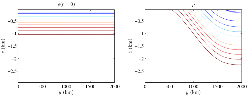
Figure 1: Initial stratification and equilibrium stratification from the spinup of the control run with $\alpha=0.1$, $\tau_{0}=0.2\ \mathrm{N}\ \mathrm{m}^{-2}$ and $\lambda=2\times 10^{-7}\ \mathrm{s}^{-1}$ for the GEOM variant (leading to an emergent $\kappa=805\ \mathrm{m}^{2}\mathrm{s}^{-1}$). The same contour levels are used for both panels.

4.2 Results

The transport associated with the equilibrium states with varying values for $\tau_{0}$ and $\lambda$ are shown in Figure 2. It is clear that CONST and VMHS^∗ show significant sensitivity of the mean transport with respect to the peak wind stress. By contrast, the ML variant shows reduced sensitivity. Notably, the GEOM variant shows very low sensitivity to varying wind stress, and thus exhibits the emergent eddy saturation, obtained in the eddy-permitting numerical experiments of Munday et al. (2013) for example. For varying eddy energy dissipation rate $\lambda$, CONST and VMHS^∗ are by construction independent of $\lambda$, while the ML and GEOM variants show increased transport with increased dissipation. These observed behavious are consistent with the analysis given in §2.2.

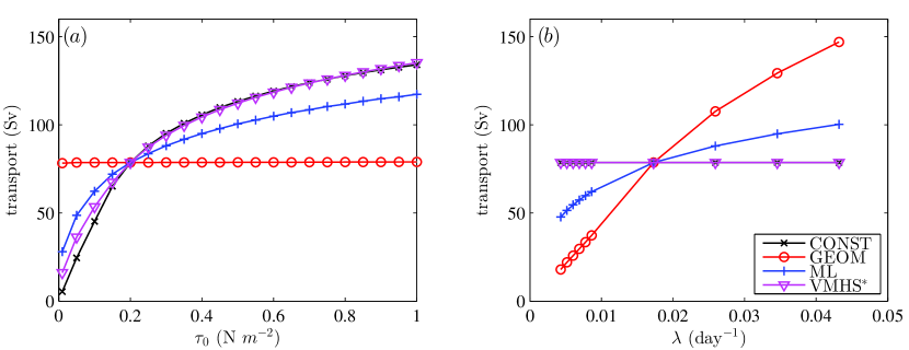
Figure 2: Transport at varying ($a$) peak wind forcing $\tau_{0}$ and ($b$) eddy energy dissipation rate $\lambda$ for the four parameterisation variants.

Denoting the domain average by

$$\langle\cdot\rangle=\frac{1}{L_{y}L_{z}}\iint(\cdot)\,\mathrm{d}y\,\mathrm{d}z,$$ (37)

the emergent $\kappa$ and $\langle E\rangle$ are shown in Figure 3. The ML and VMHS^∗ variants show a sub-linear dependence of the emergent $\kappa$ on the peak wind stress $\tau_{0}$, while the GEOM variant exhibits an almost linear dependence. For the ML and GEOM variants the emergent $\kappa$ decreases with increasing $\lambda$. The dependencies are consistent with the arguments given in §2.2. It is found here that increasing the dissipation decreases the emergent eddy energy level.

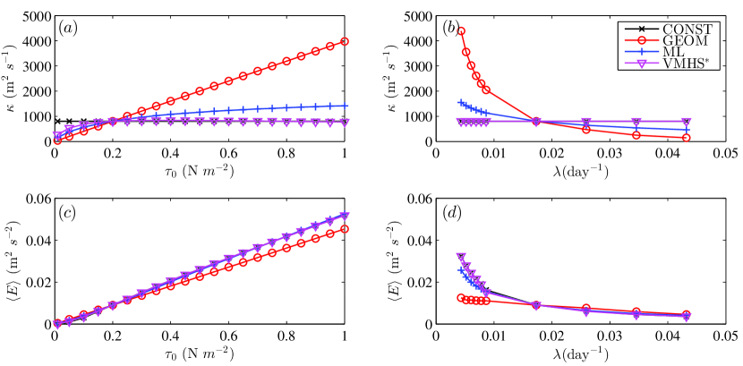
Figure 3: Emergent ($a,b$) $\kappa$ and ($c,d$) domain integrated eddy energy $\langle E\rangle$ at varying peak wind forcing $\tau_{0}$ ($a,c$) and eddy energy dissipation rate $\lambda$ ($b,d$), for the four parameterisation variants.

The emergent eddy saturation property of the GEOM variant is not limited to this parameter set. Figure 4 shows contour plots of the transport in $(\tau_{0},\lambda)$ and $(\tau_{0},\alpha)$ parameter space. As expected, there is very little dependence of the transport on $\tau_{0}$ and only at extreme parameter values is a variability seen in the contour plot. This shows robustness of the insensitivity to strength of peak wind over a large range of parameters.

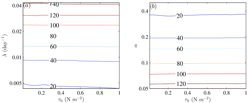
Figure 4: Contour plot of the emergent transport (in Sv) for the GEOM variant over ($a$) ($\tau_{0},\lambda$) space (with $\alpha=0.1$), and ($b$) ($\tau_{0},\alpha$) space (with $\lambda=2\times 10^{-7}\ \mathrm{s}^{-1}$).

To show how the other emergent properties of the GEOM variant depend on $\alpha$ and $\lambda$, the transport, GM coefficient, and domain averaged eddy energy over $(\lambda,\alpha)$ parameter space are shown in Figure 5. Increasing $\alpha$ increases $\kappa$ and reduces the mean transport as expected. However, the dependence of $\kappa$ on $\alpha$ is not linear, due to the indirect effect of $\alpha$ on the eddy energy. For lower values of $\alpha$, decreasing $\lambda$ leads to an increase in the eddy energy, an increase in $\kappa$, and a decrease in the mean transport. The eddy energy has a more complex dependence on $\alpha$, but for weaker dissipation increasing $\alpha$ leads to a decrease in the eddy energy. Again, these observations are consistent with the analysis given in §2.2.

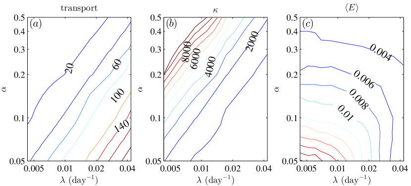
Figure 5: Contour plot of the emergent ($a$) transport (in Sv), ($b$) $\kappa$ (in $\ \mathrm{m}^{2}\ \mathrm{s}^{-1}$) and ($c$) $\langle E\rangle$ (in $\ \mathrm{m}^{2}\ \mathrm{s}^{-2}$) of the GEOM variant over $\lambda$ and $\alpha$ space, at $\tau_{0}=0.2\ \mathrm{N}\ \mathrm{m}^{-2}$. The axes are logarithmic with simulation data from 10 values of $\alpha$ ranging from $0.05$ to $0.5$ and 10 values of $\lambda$ ranging from $5\times 10^{-8}\ \mathrm{s}^{-1}$ to $5\times 10^{-7}\ \mathrm{s}^{-1}$.

5 Stratification dependent Gent–McWilliams coefficient

5.1 Implementation details

In this section a dependence of the GM coefficient on the vertical stratification is introduced, again with four variants based upon the CONST, GEOM, ML, and VMHS^∗ discussed in §3.2. The simplest CONST variant is now replaced with the form proposed in Ferreira et al. (2005)

$$\kappa=\kappa_{0}\mathcal{S},\qquad\mathcal{S}=\frac{N^{2}}{N^{2}_{\textnormal{ref}}}.$$ (38)

This imparts a vertical as well as horizontal spatial structure to the GM coefficient. In Ferreira et al. (2005) $N^{2}_{\textnormal{ref}}$ is taken to be the value of $N^{2}$ at the surface, and the $\mathcal{S}$ is tapered to a value of $1$ to avoid singularities (for example, during a convective event when outcropping occurs). Here this was found to lead to difficulties in regions of weak surface stratification, which were not alleviated by the use of clipping of $\mathcal{S}$. Instead, here a simpler approach is taken, with $N^{2}_{\textnormal{ref}}$ set equal to a constant value, for convenience set equal to $N^{2}_{\textnormal{min}}$ (see Table 1).

The GEOM variant becomes $\kappa=\kappa_{0}\mathcal{S}=\alpha E(N/M^{2})$, where again $\alpha$ is a prescribed constant. Re-arranging, integrating over the domain, and now assuming that $\kappa_{0}$ is a constant in space leads to

$$\kappa=\kappa_{0}\mathcal{S}=\left(\alpha\frac{\iint E\,\mathrm{d}y\,\mathrm{d}z}{\iint(M^{2}/N)\mathcal{S}\,\mathrm{d}y\,\mathrm{d}z}\right)\mathcal{S}.$$ (39)

The domain integrated eddy energy $\iint E\,\mathrm{d}y\,\mathrm{d}z$ is computed by solving equation (15) as before.

For the ML variant, an analogous approach yields

$$\kappa=\left(\alpha_{\tiny\mbox{ML}}\frac{\iint\sqrt{E}\,\mathrm{d}y\,\mathrm{d}z}{\iint(\mathcal{S}/L)\,\mathrm{d}y\,\mathrm{d}z}\right)\mathcal{S},$$

and use of the Cauchy–Schwarz inequality leads to

$$\kappa=\left(\alpha_{1}\frac{\sqrt{L_{y}L_{z}}\sqrt{\iint E\,\mathrm{d}y\,\mathrm{d}z}}{\iint(\mathcal{S}/L)\,\mathrm{d}y\,\mathrm{d}z}\right)\mathcal{S}.$$ (40)

Here a prescribed value for the parameter $\alpha_{1}$ is again chosen.

For the variant based on Visbeck et al. (1997), with the GM coefficient given by $\kappa=\kappa_{0}\mathcal{S}=\alpha_{\tiny\mbox{VMHS}}(M^{2}/N)L^{2}$, two forms are used. Assuming $\kappa_{0}$ is a constant in space results in the VMHS^∗ variant

$$\kappa=\left(\alpha_{2}\frac{\iint L^{2}(M^{2}/N)\,\mathrm{d}y\,\mathrm{d}z}{\iint\mathcal{S}\,\mathrm{d}y\,\mathrm{d}z}\right)\mathcal{S}.$$ (41)

Alternatively the form (32) may be used directly, resulting in the VMHS variant

$$\kappa=\alpha_{3}\frac{M^{2}}{N}L^{2},$$ (42)

where now $\alpha_{3}$ is a prescribed constant. This latter form introduces an additional explicit dependence on the local value of $M$ and the local mixing length $L$.

As for previous constant GM coefficient case, the initial state is spun up from rest first using the GEOM variant, with $\tau_{0}=0.2\ \mathrm{N}\ \mathrm{m}^{-2}$, $\lambda=2\times 10^{-7}\ \mathrm{s}^{-1}$ and $\alpha=0.1$. The initial state is the same one shown in Figure 1, and Figure 6 shows the equilibrium stratification profile and the associated spatially varying GM coefficient. This equilibrium state here has a transport of around 66 $\mathrm{Sv}$ and a domain average parameterised eddy energy of around $0.004\ \mathrm{m}^{2}\ \mathrm{s}^{-2}$. This energy is somewhat lower than the previous constant GM coefficient case, possibly due to the anticipated restriction of the parameterised eddy energy to strongly sloping isopycnals, which are confined to the upper part of the domain.

From this control run and taking the mixing length $L$ to be the Rossby deformation radius $L_{d}=NH/f_{0}$ as before for the ML and VMHS^∗ variants, the emergent $\kappa$ and end state $\overline{\rho}$ are used to calibrate $\kappa_{0}$ for CONST in (38), $\alpha_{1}$ for ML in (40) and $\alpha_{2}$ for the VMHS^∗ in (41), which are used for subsequent calculations where $\tau_{0}$ and $\lambda$ are varied. For the direct VMHS variant, the functional dependence of $\kappa$ on $M$ and $N$ differs from the functional dependence specified by $\mathcal{S}$. Here an initial value of $\alpha_{3}$ in (42) is chosen manually so that a similar transport is obtained. Other simulation details are kept the same as in Table 1 except that the convergence tolerance $\xi_{2}$ is now set to $5\times 10^{-14}$, as there is more variability given that $\kappa$ is allowed to vary over space.

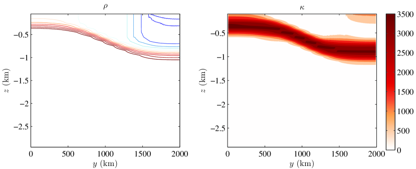
Figure 6: Equilibrium stratification and final GM coefficient distribution from control run with $\alpha=0.1$ and $\lambda=2\times 10^{-7}\ \mathrm{s}^{-1}$. The contour levels for the stratification profile are the same as for Figure 1.

5.2 Results

The resulting transport with varying $\tau_{0}$ and $\lambda$ for the five parameterisation variants is shown in Figure 7. The GEOM variant once again exhibits emergent eddy saturation behaviour. The VMHS^∗ variant and especially the ML variant also show a reduction of the sensitivity of the mean transport with respect to the peak wind stress compared to their respective case with spatially constant GM coefficient. The GEOM variant once again exhibits a strong dependence on the eddy energy dissipation rate $\lambda$. The ML variant with stratification dependence now exhibits a much weaker dependence of the transport on $\lambda$ than was observed with a constant GM coefficient case.

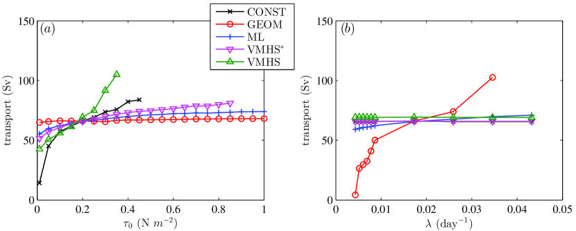
Figure 7: Transport at varying ($a$) peak wind forcing $\tau_{0}$ and ($b$) eddy energy dissipation rate $\lambda$ for the five parameterisation variants, showing only converged solutions.

Figure 8 shows the emergent $\kappa_{0}$ (defined by taking $N^{2}_{\textnormal{ref}}=5\times 10^{-6}\ \mathrm{s}^{-1}$) and $\langle E\rangle$ for varying $\tau_{0}$ and $\lambda$. The CONST and VMHS variant has $\kappa_{0}$ fixed by definition. As before, for varying $\tau_{0}$, a near linear trend of $\kappa$ with $\tau_{0}$ is seen in the GEOM variant, whilst a sub-linear trend is seen for the ML variant. Varying $\lambda$ again does not affect CONST, VMHS^∗, or VMHS by definition, while this has some effect on the ML variant and somewhat larger effect on the GEOM variant. For the ML and especially GEOM variants, increasing $\lambda$ decreases $\kappa_{0}$. Further, the eddy energy level is found to decrease with increased dissipation.

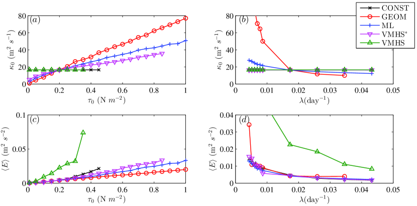
Figure 8: Emergent $\kappa_{0}$ (panel $a,b$, normalised by $N^{2}_{\textnormal{ref}}=5\times 10^{-6}$) and domain integrated eddy energy $\langle E\rangle$ (panels $c,d$) at varying peak wind forcing $\tau_{0}$ (panels $a,c$) and eddy energy dissipation rate $\lambda$ (panels $b,d$), for the five parameterisation variants. Note that the value of $\kappa_{0}$ plays no dynamical role for the VMHS variant, and is simply set to the value used for the CONST variant. Non-converged solutions have been omitted. Some data points are out of the axes range for small $\lambda$ for display reasons.

The emergent eddy saturation for the GEOM variant is again found to be robust over a range of parameters, as shown in Figure 9, though there is an increased variability with varying peak wind stress value $\tau_{0}$ at the smaller transports. Figure 10 shows contour plots of the emergent properties with varying $\lambda$ and $\alpha$. In both figures, non-converged states have been greyed out. Although showing much more variability than the analogous spatially constant $\kappa$ case in Figure 5, there is a pattern of increased transport at increasing $\lambda$ or decreasing $\alpha$, and of decreased $\kappa_{0}$ at increasing $\lambda$ or decreasing $\alpha$. Note the region with low $\lambda$ and large $\alpha$ with small transport, large $\langle E\rangle$ and thus large $\kappa_{0}$. The resulting parameterised eddies in this case are very strong, resulting in essentially flat isopycnals.

Figure 9: Contour plot of the emergent transport over ($a$) ($\tau_{0},\lambda$) space (with $\alpha=0.1$), and ($b$) ($\tau_{0},\alpha$) space (with $\lambda=2\times 10^{-7}\ \mathrm{s}^{-1}$). Regions with non-converged solutions have been greyed out and their output set to NaN.

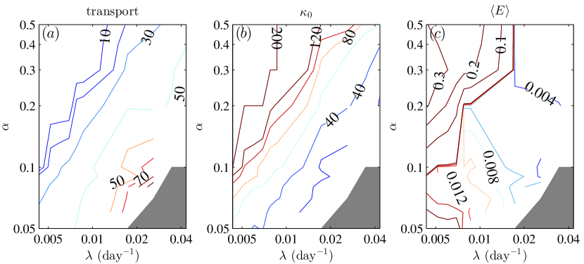
Figure 10: Contour plot of emergent ($a$) transport (in Sv), ($b$) $\kappa_{0}$ (normalised by $N^{2}_{\textnormal{ref}}=5\times 10^{-6}\ \mathrm{s}^{-1}$, in $\ \mathrm{m}^{2}\ \mathrm{s}^{-1}$) and ($c$) $\langle E\rangle$ (in $\ \mathrm{m}^{2}\ \mathrm{s}^{-2}$) of the GEOM variant over $\lambda$ and $\alpha$ space, at $\tau_{0}=0.2\ \mathrm{N}\ \mathrm{m}^{-2}$. The axes are logarithmic with simulation data from 10 values of $\alpha$ ranging from $0.05$ to $0.5$ and 10 values of $\lambda$ ranging from $5\times 10^{-8}\ \mathrm{s}^{-1}$ to $5\times 10^{-7}\ \mathrm{s}^{-1}$. Regions with non-converged solutions have been greyed out and their output set to NaN.

6 Conclusions

6.1 Summary of results

In this article the problem of emergent eddy saturation in coarse resolution ocean modelling with parameterised mesoscale eddies has been considered. Specifically, an idealised zonally averaged channel configuration was used to test the sensitivity of mean zonal transports with respect to the strength of surface wind forcing, and additionally with respect to the strength of total eddy energy dissipation and closure parameters. Variants of the Gent and McWilliams (1990) scheme have been tested, with a constant GM coefficient, a GM coefficient with a stratification dependence based upon that described in Visbeck et al. (1997), a GM coefficient with a mixing-length inspired energy dependence (e.g., Eden and Greatbatch, 2008), and a GM coefficient derived from the geometric framework described by Marshall et al. (2012). For the schemes with eddy energy dependence a parameterised equation for the domain integrated eddy energy was solved. By integrating over the domain, specific closures were derived, falling into two classes — one where the GM coefficient was spatially constant, and one where the GM coefficient had a spatial structure based upon that described in Ferreira et al. (2005). A form with additional stratification dependence, closer to the original proposal of Visbeck et al. (1997), was additionally tested.

It was found that the scheme derived from the geometric framework of Marshall et al. (2012) led to almost complete emergent eddy saturation, with little or no significant dependence of the mean transport on the surface wind stress magnitude. This was additionally observed for a wide range of eddy energy dissipation time scales and parameterisation parameter values. Moreover, it was found that the changes to the equilibrium stratification profile with different values of peak wind stress were small (not shown). This was found both for the case where the GM coefficient was spatially constant, and where the GM coefficient was assumed to depend upon the vertical stratification. Furthermore, the dependence of the transport and other emergent quantities are consistent with the physical and mathematical arguments given in §2.2. On the other hand, the use of a basic spatially and temporally constant GM coefficient led to a very significant dependence of the mean zonal transport with respect to the wind stress, similar to behaviour reported in low resolution ocean model tests described in Munday et al. (2013). Variants based upon the Visbeck et al. (1997) and upon mixing length arguments were generally found to have a somewhat reduced sensitivity, but did not exhibit full eddy saturation.

6.2 Discussion and future work

This work focuses on eddy saturation, but an equally important process that has not been investigated in this work is the ability of the GM coefficient variants in showing eddy compensation. In particular, the extent of eddy compensation depends upon both the magnitude and the location of the eddy induced transport, and the degree to which it cancels with the local Eulerian circulation (Meredith et al., 2012). The model considered in this article has no representation for ocean basins and hence is unsuitable for studying eddy compensation. An investigation into the ability of the Marshall et al. (2012) variant of the GM coefficient in showing emergent eddy compensation would require a more sophisticated eddy energy budgets than the one employed here, and is left as future work.

Assuming that the eddy energy is given via a parameterised eddy energy budget, the only remaining freedom in the Marshall et al. (2012) variant is in the specification of the non-dimensional geometric parameter $\alpha$, as all dimensional information on the magnitude of the GM coefficient is already provided by the eddy energy and mean stratification. In this work $\alpha$ was chosen to have a constant value of $0.1$, which was guided by the diagnoses of the equilibrated states in a three-layer wind forced quasi-geostrophic double gyre simulation (Marshall et al., 2012), an Eady spindown simulation of the hydrostatic primitive equations (Bachman et al., in review) as well as a Phillips-like quasi-geostrophic baroclinic jet spindown problem (Mak et al.,, in preparation). In diagnostic calculations $\alpha$ is not a constant, and in particular $\alpha$ was found in Bachman et al. (in review) to vary depending on whether the system is in a linear growth phase or in later phases of the spindown evolution. It is perhaps of theoretical interest to have $\alpha$ evolving in time to capture the initial instability, finite-amplitude regime, and transition into an equilibrated state, although this is beyond the scope of the current work.

In this paper we have found that the functional dependence for the GM coefficient proposed in Marshall et al. (2012), which incorporates energetic constraints through the solution of a parameterised eddy energy budget, yields near total emergent eddy saturation in a highly idealised configuration. For implementation in a global ocean model, since the GM scheme is normally built into the model architecture, it would appear the main additional challenge would be (i) to add a parameterised eddy energy budget that couples with the GM scheme, and (ii) derive an appropriate form for a local parameterised eddy energy budget. The domain integrated eddy energy budget employed here is much too restrictive in a global ocean model. With this, we envisage the scheme may be implemented into an operational global circulation model as follows:

1. Solve for the provisional eddy transport velocities, with a preferred vertical profile for the eddy transfer coefficient, utilising the standard GM scheme;

2. Vertically integrate the implied eddy form stress and compare with the theoretical prediction derived from the Marshall et al. (2012) geometric framework, with a prescribed non-dimensional parameter $\alpha$;

3. Solve for the parameterised, vertically integrated eddy energy budget, analogous to Eden and Greatbatch (2008) but for the full, rather than kinetic, eddy energy;

4. Rescale the eddy transport velocities, equivalent to rescaling the GM eddy transfer coefficient, uniformly over the vertical column such that the vertical integral of the eddy form stress matches the theoretical prediction from the Marshall et al. (2012) geometric framework.

By applying the energetic constraint in the vertical integral of the eddy form stresses, the recipe given above succeeds in retaining the positive-definite conversion of mean to eddy energy associated with the GM scheme, as well as the derived energetic constraint given in the Marshall et al. (2012) geometric framework.

In a closure for ocean turbulence one must typically tune the closure parameters in order to match a desired large-scale or mean state of interest. However for many key questions in physical oceanography, it is not only the mean state itself, but also the sensitivity of that mean state to external changes, which is of interest. This is, for example, critical to the understanding of the long time response of the ocean and broader climate system to long term forcing changes. The Gent–McWilliams closure is now a key component in large scale climate relevant ocean modelling, but it has been found that existing variants of the scheme in wide use, in particular with a constant Gent–McWilliams coefficient, do not yield accurate representations of ocean transport sensitivities with respect to changed in wind forcing (e.g., Farneti and Gent, 2011; Gent and Danabasoglu, 2011). This work provides the first evidence that the phenomenon of eddy saturation may be captured without major changes to the existing Gent–McWilliams closure, simply by employing the Marshall et al. (2012) form for the GM coefficient, derived from first principles with no tunable dimensional parmaeters, coupled with a parameterised eddy energy budget. A proposal on how this scheme may be implemented into a global circulation model via the addition of a parameterised eddy energy equation has been given here. Investigations into implementing this into a general circulation model, as well as theoretical developments for a parameterised eddy energy budget, are under investigation.

Appendix A Eddy energetics

In §2.1 the integrated mean energy equation is considered. Here a corresponding integrated eddy energy equation is derived.

Eddy equations, associated with the mean equations (9), are

$$\frac{\partial u^{\prime z}}{\partial t}+u\frac{\partial u^{\prime z}}{\partial x}+v\frac{\partial u^{\prime z}}{\partial y}+w\frac{\partial u^{\prime z}}{\partial z}+u^{\prime z}\frac{\partial\overline{u}^{z}}{\partial x}+v^{\prime z}\frac{\partial\overline{u}^{z}}{\partial y}+w^{\prime z}\frac{\partial\overline{u}^{z}}{\partial z}-fv^{\prime z}$$

$$\qquad~{}=-\overline{u^{\prime z}\frac{\partial u^{\prime z}}{\partial x}}^{z}-\overline{v^{\prime z}\frac{\partial u^{\prime z}}{\partial y}}^{z}-\overline{w^{\prime z}\frac{\partial u^{\prime z}}{\partial z}}^{z}-\frac{1}{\rho_{0}}\frac{\partial p^{\prime z}}{\partial x}+F^{\prime z}-D^{\prime z},$$ (43a)

$$\frac{\partial v^{\prime z}}{\partial t}+u\frac{\partial v^{\prime z}}{\partial x}+v\frac{\partial v^{\prime z}}{\partial y}+w\frac{\partial v^{\prime z}}{\partial z}+u^{\prime z}\frac{\partial\overline{v}^{z}}{\partial x}+v^{\prime z}\frac{\partial\overline{v}^{z}}{\partial y}+w^{\prime z}\frac{\partial\overline{v}^{z}}{\partial z}+fu^{\prime z}$$

$$\qquad~{}=-\overline{u^{\prime z}\frac{\partial v^{\prime z}}{\partial x}}^{z}-\overline{v^{\prime z}\frac{\partial v^{\prime z}}{\partial y}}^{z}-\overline{w^{\prime z}\frac{\partial v^{\prime z}}{\partial z}}^{z}-\frac{1}{\rho_{0}}\frac{\partial p^{\prime z}}{\partial y},$$ (43b)

$$\qquad 0=-\frac{1}{\rho_{0}}\frac{\partial p^{\prime z}}{\partial z}-\frac{g\rho^{\prime z}}{\rho_{0}}.$$ (43c)

$\left(\ldots\right)^{\prime z}$ denotes an eddy component associated with a zonal average at fixed height – for example $\rho^{\prime z}=\rho-\overline{\rho}^{z}$. It is assumed throughout this section that $f^{\prime z}=0$, and that $g$ and $\rho_{0}$ are spatially and temporally constant. In the following it is further assumed that the mean and eddy velocities $\left(0,\overline{v}^{z},\overline{w}^{z}\right)^{T}$ and $\left(u^{\prime z},v^{\prime z},w^{\prime z}\right)^{T}$ are incompressible and have zero normal component on domain boundaries.

Multiplying equation (43a) by $u^{\prime z}$, equation (43b) by $v^{\prime z}$, zonally averaging at constant height, using the hydrostatic relation (43c), and integrating over the domain, leads to the integrated eddy kinetic energy budget

$$\iint\rho_{0}K\mathrm{d}y\,\mathrm{d}z= \iint\rho_{0}\overline{u^{\prime z}\left(F^{\prime z}-D^{\prime z}\right)}^{z}\mathrm{d}y\,\mathrm{d}z$$

$$- \iint\rho_{0}\left[\frac{\partial\overline{u}^{z}}{\partial y}\overline{u^{\prime z}v^{\prime z}}^{z}+\frac{\partial\overline{u}^{z}}{\partial z}\overline{u^{\prime z}w^{\prime z}}^{z}+\frac{\partial\overline{v}^{z}}{\partial y}\overline{v^{\prime z}v^{\prime z}}^{z}+\frac{\partial\overline{v}^{z}}{\partial z}\overline{v^{\prime z}w^{\prime z}}^{z}\right]\mathrm{d}y\,\mathrm{d}z,$$

$$- \iint g\overline{w^{\prime z}\rho^{\prime z}}^{z}\mathrm{d}y\,\mathrm{d}z,$$ (44)

with eddy kinetic energy (per unit volume)

$$\rho_{0}K=\frac{1}{2}\rho_{0}\overline{u^{\prime z}u^{\prime z}}^{z}+\frac{1}{2}\rho_{0}\overline{v^{\prime z}v^{\prime z}}^{z}.$$ (45)

Now from the density equation

$$\frac{\partial\rho}{\partial t}+\frac{\partial\left(u\rho\right)}{\partial x}+\frac{\partial\left(v\rho\right)}{\partial y}+\frac{\partial\left(w\rho\right)}{\partial z}=0,$$ (46)

multiplying by the height $z$, zonally averaging at constant height, and integrating over the domain, leads to

$$\iint\overline{w^{\prime z}\rho^{\prime z}}^{z}\mathrm{d}y\,\mathrm{d}z =\iint\frac{\partial\left(\overline{\rho}^{z}z\right)}{\partial t}\mathrm{d}y\,\mathrm{d}z-\iint\overline{w}^{z}\overline{\rho}^{z}\mathrm{d}y\,\mathrm{d}z$$

$$=\iint\frac{\partial\left(\overline{\rho}^{\rho}z\right)}{\partial t}\mathrm{d}y\,\mathrm{d}z-\frac{\partial\left(\overline{\rho}^{*}z\right)}{\partial t}\mathrm{d}y\,\mathrm{d}z-\iint\overline{w}^{z}\overline{\rho}^{z}\mathrm{d}y\,\mathrm{d}z,$$ (47)

where $\rho^{*}=\overline{\rho}^{\rho}-\overline{\rho}^{z}$ is the difference between the two mean densities. Assuming that the eddy transport velocity $\left(0,v^{*},w^{*}\right)^{T}$ has zero normal component on domain boundaries, multiplying equation (2) by the height $z$ and integrating over the domain yields

$$\iint\frac{\partial\left(\overline{\rho}^{\rho}z\right)}{\partial t}\mathrm{d}y\,\mathrm{d}z=\iint\hat{w}\overline{\rho}^{\rho}\mathrm{d}y\,\mathrm{d}z.$$ (48)

Combining equations (A), (A), and (48) leads to the integrated eddy energy budget

$$\frac{\mathrm{d}}{\mathrm{d}t}\iint\rho_{0}E\mathrm{d}y\,\mathrm{d}z =\iint\rho_{0}\overline{u^{\prime z}\left(F^{\prime z}-D^{\prime z}\right)}^{z}\mathrm{d}y\,\mathrm{d}z$$

$$-\iint\rho_{0}\left[\frac{\partial\overline{u}^{z}}{\partial y}\overline{u^{\prime z}v^{\prime z}}^{z}+\frac{\partial\overline{u}^{z}}{\partial z}\overline{u^{\prime z}w^{\prime z}}^{z}+\frac{\partial\overline{v}^{z}}{\partial y}\overline{v^{\prime z}v^{\prime z}}^{z}+\frac{\partial\overline{v}^{z}}{\partial z}\overline{v^{\prime z}w^{\prime z}}^{z}\right]\mathrm{d}y\,\mathrm{d}z$$

$$-\iint w^{*}g\overline{\rho}^{\rho}\mathrm{d}y\,\mathrm{d}z-\iint\overline{w}^{z}g\rho^{*}\mathrm{d}y\,\mathrm{d}z,$$ (49)

with total eddy energy (per unit volume)

$$\rho_{0}E=\frac{1}{2}\rho_{0}\overline{u^{\prime z}u^{\prime z}}^{z}+\frac{1}{2}\rho_{0}\overline{v^{\prime z}v^{\prime z}}^{z}-\rho^{*}gz.$$ (50)

The first right-hand-side term in equation (A) is the eddy energy generation due to forcing in the horizontal momentum equations. The second right-hand-side term is the mean-to-eddy energy conversion due to the eddy Reynolds stresses. The third right-hand-side term is the mean-to-eddy energy generation due to the eddy transport velocity, and corresponds exactly to the conversion term appearing in the mean energy equation (10). The final term is an additional conversion term which arises from the direct application of an average at constant height to the hydrostatic relation (see the discussion in McDougall and McIntosh, 2001, appendix B). Replacing $\overline{\rho}^{\rho}$ with $\overline{\rho}^{z}$ in equation (9c) would lead to the appearance of a corresponding term in the integrated mean energy equation.

Appendix B Deriving equation (21)

If both the GM coefficient and the eddy energy dissipation scale with the eddy energy, then there is an apparent degeneracy in the eddy energy equation (15). If, for example, the scaling factors are constant, then the integrated eddy energy can be factored out, leading to a balance between the rates of eddy energy generation and dissipation. In this appendix this property is formalised somewhat via the use of appropriate integral inequalities.

It is assumed that functions $f$ and $g$ are suitably smooth such that Hölder’s inequality (e.g., Doering and Gibbon, 1995, Appendix A)

$$\left\|fg\right\|_{L^{1}}\leq\left\|f\right\|_{L^{p}}\left\|g\right\|_{L^{q}},\qquad\left\|f\right\|_{L^{p}}=\left(\int_{\Omega}|f|^{p}\,\mathrm{d}\Omega\right)^{1/p},\qquad\frac{1}{p}+\frac{1}{q}=1,$$

may be applied. Choosing the Hölder conjugates $p=2$ and $q=2$ (i.e. a generalised Cauchy–Schwartz inequality) and applying the above inequality to the steady state eddy energy equation (15) leads to

$$\lambda\left\|E\right\|_{L^{1}}\leq\alpha\left\|E\right\|_{L^{2}}\left\|\frac{|f|\rho_{0}}{gN}\left|\frac{\partial\overline{u}^{z}}{\partial z}\right|\right\|_{L^{2}}.$$ (51)

Notice that the $L^{1}$ norm is the integral of the absolute value, and so $\left\|E\right\|_{L^{1}}=\iint E\,\mathrm{d}y\,\mathrm{d}z$. From this, it follows that

$$\frac{\lambda}{\alpha}\frac{\|E\|_{L^{1}}}{\|E\|_{L^{2}}}=\tilde{C}\left\|\frac{|f|\rho_{0}}{gN}\left|\frac{\partial\overline{u}^{z}}{\partial z}\right|\right\|_{L^{2}},$$ (52)

for $\tilde{C}\in(0,1]$. Although $\|E\|_{L^{1}}\leq\|E\|_{L^{2}}$ (a consequence of Hölder’s inequality), if $\|E\|_{L^{1}}\approx\|E\|_{L^{2}}$ then the relation (21) results.

Some more progress may be made if the norms of the derivatives may be assumed to be small. Assuming a bounded Lipschitz domain, the $\left\|E\right\|_{L^{2}}$ term may be controlled by utilising the Gagliardo–Nirenberg interpolation inequality (Nirenberg 1959, §2; see also Appendix A of Doering and Gibbon 1995), which states that

$$\|\mathrm{D}^{j}f\|_{L^{p}}\leq C_{1}\|\mathrm{D}^{m}f\|_{L^{r}}^{a}\|f\|_{L^{q}}^{1-a}+C_{2}\|f\|_{L^{s}},\qquad\frac{1}{p}=\frac{j}{d}+\left(\frac{1}{r}-\frac{m}{d}\right)a+\frac{1-a}{q}$$

with $\mathrm{D}$ being a weak derivative, $d$ is the dimensionality of the domain, $1\leq r,q\leq\infty$, $j/m\leq a\leq 1$, and $s>0$ is arbitrary. This does not cover some exceptional cases, though they are not of interest here. The constants $C_{1,2}$ only depend on the domain and the choice of the parameter values. For $d=2$ here, taking $j=0$, $p=2$ and $s=1$, it is noted that $m=1$, $r=1$ and $a=1$ is one option (which is a form of the Sobolev inequality; e.g., Evans 1998, §5.6.1), and taking $s=1$ and $f=E$ results in

$$\|E\|_{L^{2}}\leq C_{1}\|\mathrm{D}E\|_{L^{1}}+C_{2}\|E\|_{L^{1}}.$$

If $m=1$, $r=2$, $a=1/2$ and $q=1$ instead, then

$$\|E\|_{L^{2}}\leq C_{1}\|\mathrm{D}E\|_{L^{2}}^{1/2}\|E\|_{L^{1}}^{1/2}+C_{2}\|E\|_{L^{1}},$$

which is analogous to the inequality of Nash (1958). Other possibilities exist involving higher derivatives. Either way, assuming that the terms involving the derivatives are small compared to $C_{2}\|E\|_{L^{1}}$, then the relation (21) again follows, with a constant of proportionality that only depends on the domain and the parameter values chosen in the Gagliardo–Nirenberg interpolation inequality and is bounded away from zero and infinity.

The Gagliardo–Nirenberg inequality may be applied again to further control the term involving the derivative in terms of higher $L^{p}$ norms, although the relation again needs further assumptions. Hölder’s inequality with the conjugates $p=1$ and $q=\infty$ could be applied at the beginning to factor out $\|E\|_{L^{1}}$ immediately, however there is then a lack of control on the $L^{\infty}$ norm as the Gagliardo–Nirenberg inequality above does not apply. An alternative approach may be to consider adding and subtracting the mean of the relevant function and apply the Minkowski inequality (a generalised triangle inequality) which would yield similar results. This approach when applied to the ML variant $\kappa=\alpha_{\tiny\mbox{ML}}$ does not appear to yield the same bound as the eddy energy equation does not become degenerate.

References

- Andrews (1983) Andrews, D. G., 1983. A finite-amplitude Eliassen-Palm theorem in isentropic coordinates. J. Atmos. Sci. 40, 1877–1883.
- Arakawa and Lamb (1977) Arakawa, A., Lamb, V. R., 1977. Computational design of the basic dynamical processes of the ucla general circulation model. Methods Comput. Phys. 17, 173–265.
- Bachman et al. (in review) Bachman, S. D., Marshall, D. P., Maddison, J. R., Mak, J., in review. Evaluation of a scalar transport coefficient based on geometric constraints. Ocean Modell.
- Cessi (2008) Cessi, P., 2008. An energy-constrained parametrization of eddy buoyancy flux. J. Phys. Oceanogr. 38, 1807–1819.
- Courant et al. (1928) Courant, R., Friedrichs, K., Lewy, H., 1928. Ueber die partiellen Differenzengleichungen der mathematischen Physik. Mathematische Annalen 100 (1), 32–74.
- Cox (1987) Cox, M. D., 1987. Isopycnal diffusion in a -coordinate ocean model. Ocean Modelling (unpublished manuscripts) 74, 1–5.
- Danabasoglu and Marshall (2007) Danabasoglu, G., Marshall, J., 2007. Effects of vertical variations of thickness diffusivity in an ocean general circulation model. Ocean Modell. 18, 122–141.
- Danabasoglu et al. (1994) Danabasoglu, G., McWilliams, J. C., Gent, P. R., 1994. The role of mesoscale tracer transports in the global ocean circulation. Science 264, 1123–1126.
- Doering and Gibbon (1995) Doering, C. R., Gibbon, J. D., 1995. Applied analysis of the Navier–Stokes Equations. Cambridge University Press.
- Eden and Greatbatch (2008) Eden, C., Greatbatch, R. J., 2008. Towards a mesoscale eddy closure. Ocean Modell. 20, 223–239.
- Evans (1998) Evans, L. C., 1998. Partial differential equations. American Mathematical Society.
- Farneti and Delworth (2010) Farneti, R., Delworth, T. L., 2010. The role of mesoscale eddies in the remote oceanic response to altered Southern Hemisphere winds. J. Phys. Oceanogr. 40, 2348–2354.
- Farneti and Gent (2011) Farneti, R., Gent, P. R., 2011. he effects of the eddy-induced ad- vection coefficient in a coarse-resolution coupled climate model. Ocean Modell. 39, 135–145.
- Ferreira et al. (2005) Ferreira, D., Marshall, J., Heimbach, P., 2005. Estimating eddy stresses by fitting dynamics to observations using a residual-mean ocean circulation model and its adjoint. J. Phys. Oceanogr. 35, 1891–1910.
- Fyfe et al. (2007) Fyfe, J. C., Saneko, O. A., Zickfield, K., Eby, M., Weaver, A. J., 2007. The role of poleward-intensifying winds on Southern Ocean warming. J. Climate 20, 5391–5400.
- Gent and Danabasoglu (2011) Gent, P. R., Danabasoglu, G., 2011. Response to increasing southern hemisphere winds in CCSM4. J. Climate 24, 4992–4998.
- Gent and McWilliams (1990) Gent, P. R., McWilliams, J. C., 1990. Isopycnal mixing in ocean circulation models. J. Phys. Oceanogr. 20, 150–155.
- Gent et al. (1995) Gent, P. R., Willebrand, J., McDougall, T. J., McWilliams, J. C., 1995. Parameterizing eddy-induced tracer transports in ocean circulation models. J. Phys. Oceanogr. 25, 463–474.
- Hallberg and Gnanadesikan (2006) Hallberg, R., Gnanadesikan, A., 2006. The role of eddies in determining the structure and response of the wind-driven Southern Hemisphere overturning: Results from the Modeling Eddies in the Southern Ocean (MESO) projects. J. Phys. Ocenogr. 36, 2232–2252.
- Hogg and Blundell (2006) Hogg, A. M., Blundell, J. R., 2006. Interdecadal variability of the Southern Ocean. J. Phys. Oceanogr. 36, 1626–1645.
- Hogg and Meredith (2006) Hogg, A. M., Meredith, M. P., 2006. Circumpolar response of Southern Ocean eddy activity to a change in the Southern Annular Mode. Geophys. Res. Lett. 33, L16608.
- Hogg et al. (2008) Hogg, A. M., Meredith, M. P., Blundell, J. R., Wilson, C., 2008. Eddy heat flux in the Southern Ocean: Response to variable wind forcing. J. Climate 21, 608–620.
- Hogg and Munday (2014) Hogg, A. M., Munday, D. R., 2014. Does the sensitivity of Southern Ocean circulation depend upon bathymetric details? Phil. Trans. R. soc. A 372, 2010050.
- Jansen et al. (2015) Jansen, M. F., Adcroft, A. J., Hallberg, R., Held, I. M., 2015. Parameterization of eddy fluxes based on a mesoscale energy budget. Ocean Modell. 92, 28–41.
- Larichev and Held (1995) Larichev, V. D., Held, I. M., 1995. Eddy amplitudes and fluxes in a homogeneous model of fully developed baroclinic instability. J. Phys. Oceanogr. 25 (10), 2285–2297.
- Marshall (1997) Marshall, D. P., 1997. Subduction of water masses in an eddying ocean. J. Mar. Res. 55, 201–222.
- Marshall et al. (submitted) Marshall, D. P., Ambaum, M. H. P., Maddison, J. R., Munday, D. R., Novak, L., submitted. Understanding ocean eddy saturation and its surprising consequences. Nature.
- Marshall et al. (2012) Marshall, D. P., Maddison, J. R., Berloff, P. S., 2012. A framework for parameterizing eddy potential vorticity fluxes. J. Phys. Oceanogr. 42, 539–557.
- McDougall and McIntosh (2001) McDougall, T. J., McIntosh, P. C., 2001. The temporal-residual-mean velocity. Part II: Isopycnal interpretation and the tracer and momentum equations. J. Phys. Oceanogr. 31, 1222–1246.
- Meredith et al. (2012) Meredith, M. P., Garabato, A. C. N., Hogg, A. M., Farneti, R., 2012. Sensitivity of the overturning circulation in the Southern Ocean to decadal changes in wind forcing. J. Climate 25, 99–110.
- Munday et al. (2013) Munday, D. R., Johnson, H. L., Marshall, D. P., 2013. Eddy saturation of equilibrated circumpolar currents. J. Phys. Oceanogr. 43, 507–532.
- Nash (1958) Nash, J., 1958. Continuity of solutions of parabolic and elliptic equations. Amer. J. Math. 80, 931–954.
- Nirenberg (1959) Nirenberg, L., 1959. On elliptic partial differential equations. Ann. Sculoa Norm. Sup. Pisa 13, 115–162.
- Redi (1982) Redi, M. H., 1982. Oceanic isopycnal mixing by coordinate rotation. J. Phys. Oceanogr. 12, 1154–1158.
- Straub (1993) Straub, D. N., 1993. On the transport and angular momentum balance of channel models of the Antarctic Circumpolar Current. J. Phys. Oceanogr. 23, 776–782.
- Viebahn and Eden (2012) Viebahn, J., Eden, C., 2012. Standing eddies in the Meridional Overturning Circulation. J. Phys. Oceanogr. 42, 1496–1508.
- Visbeck et al. (1997) Visbeck, M., Marshall, J., Haine, T., Spall, M., 1997. Specification of eddy transfer coefficients in coarse-resolution ocean circulation models. J. Phys. Oceanogr. 27, 381–402.
- Young (2012) Young, W. R., 2012. An exact thickness-weighted average formulation of the Boussinesq equations. J. Phys. Oceanogr. 42, 692–707.