Nonlinear response of inertial tracers in steady laminar flows:
differential and absolute negative mobility

Abstract

We study the mobility and the diffusion coefficient of an inertial tracer advected by a two-dimensional incompressible laminar flow, in the presence of thermal noise and under the action of an external force. We show, with extensive numerical simulations, that the force-velocity relation for the tracer, in the nonlinear regime, displays complex and rich behaviors, including negative differential and absolute mobility. These effects rely upon a subtle coupling between inertia and applied force which induce the tracer to persist in particular regions of phase space with a velocity opposite to the force. The relevance of this coupling is revisited in the framework of non-equilibrium response theory, applying a generalized Einstein relation to our system. The possibility of experimental observation of these results is also discussed.

Introduction.– Understanding the response of a system to an external stimulus from the observation of the unperturbed dynamics, represents a central issue in statistical mechanics. For weak perturbations of an equilibrium state, the fluctuation-dissipation theorem (FDT) solves the problem, expressing the system response in terms of correlation functions kubo . Generalizations of this result have been recently derived, to address the much more complex issue of predicting the response in nonequilibrium conditions CR03 ; CLZ07 ; MPRV08 ; seifert ; BM13 , when detailed balance does not hold and currents cross the system, or in the nonlinear response regime, where higher order response functions have to be taken into account BB05 ; LCSZ08 ; D12 . All these approaches point out the role played by the coupling among degrees of freedom which emerges out of equilibrium, adding extra-terms to the standard FDT SS06 ; VBPV09 ; SVGP10 ; C11 ; GPSV14 .

A paradigmatic problem within such a nonlinear response theory is concerned with the dynamics of a tracer particle, traveling in a complex medium under the action of an external field $F$. In particular, one is interested in the force-velocity relation $v(F)$, or the mobility $\mu(F)=v(F)/F$, and the diffusion coefficient $D(F)$ of the tracer particle. These curves can be strongly affected by the interaction between the tracer and the surrounding medium, and can show striking nonlinear behaviors. This kind of problem has originated in the field of active microrheology of complex fluids, such as emulsions, suspensions, polymer, and micellar solutions SM09 ; PV14 , where information on the structure of the host medium is inferred from the motion of a biased probe embedded in it. In this context inertia is usually negligible, whereas the force-velocity relation in non-overdamped systems, which play an important role in fluid dynamics TB09 , seems much less studied.

One of the surprising effects observed in the force-velocity relation of several models of biased tracers in nonequilibrium systems is a negative differential mobility (NDM). This means that the tracer velocity, after increasing linearly according to linear response, displays a nonmonotonic behavior, characterized by a maximum for a certain value of the external driving field. Just beyond this value, the differential mobility $d\mu/dF$ becomes negative, implying a slowing down of the particle motion at increasing force. This kind of phenomenon, denoted with the telling expression “getting more from pushing less”, has been explained for nonequilibrium toy models in royce and can be observed in different systems, such as Brownian motors CM96 , kinetically constrained models of glass formers JKGC08 ; S08 and driven lattice gases LF13 ; BM14 ; BIOSV14 ; BSV15 ; BIOSV16 , where analytic approaches are possible LF13 ; BIOSV14 ; BIOSV16 . In most of the aforementioned systems the non-linear behavior is due to a reciprocal tracer-medium interaction, i.e. the tracer not only feels the action of the solvent but influences it, modifying its microstructure. More generally, within the framework of nonequilibrium statistical mechanics, the occurrence of NDM has been related to the concept of dynamical activity of the tracer, which is a measure of time-symmetric currents and expresses a “jitteriness” of the particle during its motion BBMS13 ; BM14 ; M16 .

Even more surprisingly, there exist cases of absolute negative mobility (ANM), $\mu<0$, where the particle travels against the external force. This phenomenon can be realized in specific models, due the carefully tuned coupling between colored noise, asymmetric spatial structures, and driving field RERDRA05 ; KMHLT06 ; MKTLH07 ; ERAR10 .

In this Letter we show that these kinds of behaviors can take place in more realistic inertial tracer models, relevant in fluid dynamics. In particular, we investigate the linear and nonlinear response of an inertial particle moving in a steady (incompressible) cellular velocity field, under the action of an external force, and subject to thermal agitation. The presence of inertia implies a non-trivial deviation of the particle’s motion from the trajectory of a fluid particle, typically leading to the appearance of strongly inhomogeneous distributions – a phenomenon known as preferential concentration or particle clustering BBCLMT07 ; CCLT08 . This can be responsible for an enhanced probability of chemical, biological or physical interaction, as for instance, for the time scales of rain F02 , sedimentation speed under gravity LCLV08 , or the planetesimals formation in the early Solar System B99 . Here we discover that such a preferential concentration strongly depends upon the external force, leading to a rich non-linear behavior for the average particle’s velocity, showing NDM and, in particular cases, even ANM. By an analysis of the tracer’s trajectories we identify a possible mechanism responsible for such behaviors. Moreover we interpret our results within the framework of nonequilibrium response theory, exploiting a generalized Einstein relation (GER), derived recently in BBMW10 ; BMW11 , which makes clear the role played by the coupling between the velocity field and the tracer dynamics.

The model.– We consider the following equations of motion of an inertial tracer particle in two dimensions, with spatial coordinates $(x,y)$ and velocities $(v_{x},v_{y})$, subject to an external force $F$ along the $x$ direction, and traveling through a divergenceless cellular flow $(U_{x},U_{y})$

$$\dot{x} = v_{x},\qquad\dot{y}=v_{y}$$ (1)

$$\dot{v}_{x} = -\frac{1}{\tau}(v_{x}-U_{x})+F+\sqrt{2D_{0}}\xi_{x}$$ (2)

$$\dot{v}_{y} = -\frac{1}{\tau}(v_{y}-U_{y})+\sqrt{2D_{0}}\xi_{y}$$ (3)

$$U_{x} = \frac{\partial\psi(x,y)}{\partial y},\qquad U_{y}=-\frac{\partial\psi(x,y)}{\partial x}.$$ (4)

Here $\psi(x,y)=LU_{0}/(2\pi)\sin(2\pi x/L)\sin(2\pi y/L)$ is the stream function and $\xi_{x}$ and $\xi_{y}$ are uncorrelated white noises with zero mean and unitary variance. The velocity field here considered corresponds to two-dimensional convection and shows a very rich behavior YPP89 ; CMMV99 . In addition, it can be easily realized in a laboratory, e.g. with rotating cylinders SG88 or in ion solutions in array of magnets T02 . Let us stress that our system, even in the absence of external driving $F$, is out of equilibrium because of the steady velocity field represented by the non-gradient forces of Eq. (4). In what follows we measure length and time in units of $L$ and $L/U_{0}$ respectively, setting therefore $U_{0}=1$ and $L=1$, which defines a typical time scale of the flow $\tau^{*}=L/U_{0}=1$. Another important ingredient of our model is the presence of microscopic noise with molecular diffusivity $D_{0}$, which guarantees ergodicity and is related to the temperature $T$ of the environment by $D_{0}=T/\tau$ nota0 . We stress that, in the presence of an advection field, the statistic of the phase space explored by the tracer, $\{x(t),y(t),v_{x}(t),v_{y}(t)\}$, even at $F=0$, depends on both $\tau$ and $D_{0}$ in a nontrivial way, and the finite value of $\tau$ has an important role for the concentration properties BBCLMT07 . When $\tau\to 0$ (fluid particle limit, where the tracer evolves according to the equation $\dot{\boldsymbol{x}}=\boldsymbol{U}+\sqrt{2D}\boldsymbol{\xi}$ with $D$ an effective diffusivity), because of $\boldsymbol{U}=(U_{x},U_{y})$ incompressibility, the tracer visits the two-dimensional phase space in a uniform way nota . The same happens for $\tau\to\infty$, when the tracer is insensitive to the field and uniformly diffuses through the flow.

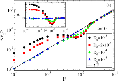
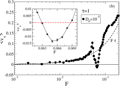
Figure 1: (a) Force-velocity relation $\langle v_{x}\rangle(F)$ and mobility $\mu$ (inset) for different values of $D_{0}$, in the case $\tau=10$. NDM is observable for $D_{0}=10^{-5}$ and $D_{0}=2\cdot 10^{-5}$, around $F\sim 4\cdot 10^{-3}$. (b) Force-velocity relation $\langle v_{x}\rangle(F)$ in the case $\tau=1$ for $D_{0}=10^{-5}$. Notice the negative peak, corresponding to ANM, observed in a range of forces near $F\sim 6.5\cdot 10^{-2}$, which is magnified in the inset.

Negative differential and absolute mobility.– Here we are mainly interested in the behavior of the stationary velocity $\langle v_{x}\rangle=\tau F+\langle U_{x}[x(t),y(t)]\rangle$, where $\langle\cdot\rangle$ denotes averages over trajectories of the particle with different initial conditions and noise realizations. We first consider the case $\tau>\tau^{*}$. In Fig. 1(a) we show, as a function of $F$, $\langle v_{x}\rangle$ and the mobility $\mu=\langle v_{x}\rangle/F$ (inset), for $\tau=10$ and different values of $D_{0}$, as computed in numerical simulations numsim . A linear regime at small forces, characterized by a constant mobility depending on $D_{0}$, is followed by a complex nonlinear scenario which emerges at intermediate values of the force. In particular, a nonmonotonic behavior corresponding to NDM takes place, with a maximum that slightly shifts and then disappears as $D_{0}$ is increased. This is expected because if the noise is strong enough the effect of the velocity field $\boldsymbol{U}$ is averaged out. The same happens for large enough forces, for which again the effect of the velocity field $\boldsymbol{U}$ is negligible and, irrespective of $D_{0}$, the trivial behavior $\langle v_{x}\rangle(F)=\tau F$ is recovered. Notice that this asymptotic linear behavior is different from the saturation effect at large force usually observed in lattice gas models BIOSV14 .

An even more striking phenomenon is observed in cases with $\tau\sim\tau^{*}$. In Fig. 1(b) we show the force-velocity relation for $\tau=1$: Again a complex nonlinear behavior can be observed for intermediate values of $F$ and, surprisingly, ANM (i.e. $\langle v_{x}\rangle/F<0$) is observed in a range around $F\sim 0.065$.

In order to get insight into the origin of the observed NDM and ANM, we have studied typical trajectories of the tracer as reported in Fig. 2. In panel (a) we show that the motion of our tracers is realized along preferential “channels” which are aligned to two main directions: some of these channels are characterized by $\langle v_{x}\rangle<0$ (we call them “leftward”) and others by $\langle v_{x}\rangle>0$ (called in the following “rightward”). These preferential channels are seen for not too strong values of the noise (roughly up to values $D_{0}\sim 10^{-4}$) and independently of the value of the force, but disappear reducing inertia. Both inertia and noise activate random transitions between the channels MKTLH07 . The force induces a bias in such transitions, determining, in general, an average $\langle v_{x}\rangle\neq 0$. In panel (b) we show a mechanism for explaining how an increase of the positive force may enhance the probability of transitions from rightward channels to leftward channels, which can lead to NDM or even ANM. The reasoning is the following. Initially the particle is travelling along a rightward channel. For the chosen $F=0.065$ (black arrows), it occurs that the particle is pushed from region “A” to region “B” where the underlying velocity field is strongly negative: a transition to a leftward channel is then realized. With a smaller (green arrows) or larger (cyan arrows) force, the particle avoids the adverse region “B” and continues its run along rightward channels. This suggests that there exists a range of forces for which the tracer is induced to visit more frequently channels with velocity opposite to the force. Depending on how much this effect is pronounced, NDM or ANM can occur.

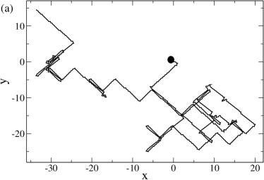
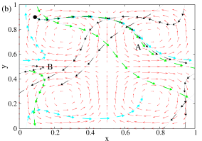
Figure 2: Samples of the tracer’s trajectories for $\tau=1$, $F=0.065$, $D_{0}=0$. (a) History of the particle’s position $(x,y)$, recorded for a time-length $760\tau^{*}$, starting near $(0,0)$ (marked as a black spot); (b) the black arrows represent the same trajectory for a timelength $\sim 10\tau^{*}$ (folded into a single cell, for the purpose of visualization), the green and cyan arrows start with the same initial condition but are realized with $F=0.04$ and $F=0.09$ respectively, and the red arrows illustrate the underlying velocity field.

Diffusivity– Next we focus on the study of the diffusion coefficient $D_{x}(F)$, defined as

$$D_{x}=\lim_{t\to\infty}\frac{1}{2t}[\langle x(t)^{2}\rangle-\langle x(t)\rangle^{2}],$$ (5)

in order to understand how the FDT is modified in our system. Here we consider the case $\tau=10$ (other cases show similar behaviors), which is reported in Fig. 3(a). Notice that $D_{x}$ is nearly independent of the force at small forces and at large forces, where it coincides with the value expected in the absence of the velocity field, $D_{x}=\tau^{2}D_{0}$. It is remarkable that $\lim_{F\to 0}D_{x}\gg\lim_{F\to\infty}D_{x}$: such a discrepancy decreases when $D_{0}$ is increased. In order to better understand the role of the molecular diffusivity $D_{0}$ in our system, in the inset of Fig. 3(a) we report the behavior of $D_{x}(F=0)$ as a function of $D_{0}$. For large enough noise amplitude, the scaling is linear, as expected, because the diffusion coefficient is dominated by the microscopic diffusivity. On the contrary, for $D_{0}\to 0$, the particle diffusivity diverges, similarly to what found by Taylor Taylor for the dispersion of a fluid particle in laminar flows in straight channels. In the case of Taylor diffusion of a fluid particle in a shear flow, the behavior $D_{x}\sim D_{0}^{-1}$ can be easily understood in terms of long horizontal ballistic motion, the duration of which increases as $D_{0}$ decreases. In our system the understanding is not so simple, but the divergence $D_{x}\sim D_{0}^{-\alpha}$ and the long channels observed in Fig. 2(a) suggest a similar scenario.

Generalized Einstein relation.– The behaviors described above can be interpreted within the context of response theory. In equilibrium conditions, and in the linear regime, the Einstein relation predicts a proportionality between the mobility and the diffusivity, via the inverse temperature

$$\mu=\mu_{0}\equiv\frac{1}{T}D_{x}.$$ (6)

In our system, the presence of the velocity field $\boldsymbol{U}$ introduces significant nonequilbirium effects that are clearly visible in Fig. 3(b), where we report the measured mobility $\mu$ rescaled by $\mu_{0}$. Only for large enough values of $F$, where the effect of $\boldsymbol{U}$ is negligible and the system can be considered at equilibrium, the ratio $\mu/\mu_{0}\sim 1$. Eventually, for $D_{0}$ large enough, the noise makes the velocity field irrelevant and $\mu/\mu_{0}\sim 1$ in all regimes.

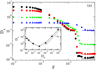
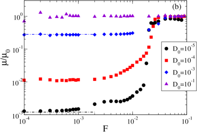
Figure 3: (a) Tracer diffusivity $D_{x}(F)$ for different values of $D_{0}$ (see legend of Fig. 1(a)) with $\tau=10$. The continuous lines represent the values $\tau^{2}D_{0}$. In the inset it is plotted $D_{x}(F=0)$ as a function of the microscopic diffusivity $D_{0}$. (b) Mobility $\mu$ over $\mu_{0}=D_{x}/T$, for $\tau=10$. The dot-dashed lines represent the predictions of the GER in two cases.

The difference due to nonequilibrium effects can be revisited in terms of a GER, derived for systems in out-of-equilibrium steady states. According to this relation, the particle mobility can be expressed as the sum of two contributions: one proportional to the diffusion coefficient, as in the standard Einstein relation (6), and the other involving the correlation function with the time-integral of the velocity field $U_{x}$, computed along the trajectory of the particle. As discussed in detail in BMW11 , for a system described by a set of stochastic equations as in Eqs. (1-4), the GER explicitly reads

$$\lim_{F\to 0}\mu(F)=\frac{1}{T}[D_{x}(F=0)-C_{x\Phi}(F=0)]$$ (7)

$$C_{x\Phi}(F)=\lim_{t\to\infty}\frac{1}{2Tt}\langle[x(t)-x(0)]\Phi(t)\rangle_{c,F},$$ (8)

where

$$\Phi(t)=\int_{0}^{t}U_{x}[x(s),y(s)]ds,$$ (9)

and $\langle A(t)B(s)\rangle_{c,F}=\langle A(t)B(s)\rangle_{F}-\langle A\rangle_{F}\langle B\rangle_{F}$ is the connected correlation function measured at force $F$. We have computed in numerical simulations the nonequilibrium contribution due to the coupling with the field $\Phi$. The validity of the predictions of the GER (8) is shown - as dot-dashed lines - in Fig. 3(b), for two cases at $D_{0}=10^{-5}$ and $D_{0}=10^{-3}$. Let us stress that Eq. (8) can be exploited also at non-vanishing forces: indeed the differential mobility $d\langle v_{x}\rangle/dF$ at a finite value of $F$ is given by the same expression, by measuring the two terms $D_{x}$ and $C_{x\Phi}$ at force $F$. The prediction of GER for $d\langle v_{x}\rangle/dF$ is negative where NDM appears, as we checked numerically: NDM therefore can be interpreted as the consequence of $C_{x\Phi}$ becoming larger than $D_{x}$ BM14 . Also in the case $\tau=1$, for the force values with ANM, the GER is verified, showing strong negative and positive differential mobilities just before and just after the minimum of $\langle v_{x}\rangle(F)$.

Conclusions.– We have studied the effects of a driving external force on the dynamics of an inertial particle advected by a velocity field, in the nonlinear regime. We have discovered nontrivial behaviors of the stationary tracer velocity and of its diffusivity as a function of the force, such as NDM and ANM. These effects are due to a complicated combined action of the applied force, the particle inertia and the underlying velocity field. It turns out that, in some force regimes, this coupling leads the tracer to persist in regions of the velocity field which drag it against the force direction, resulting in a slowing down of the tracer velocity, or even producing a negative mobility nota1 . The central role played by the coupling with the velocity field clearly emerges in the GER which is satisfied in our nonequilibrium system. The striking behaviors shown by the model should be observable in experiments with biased inertial tracers in laminar flows, realized, for instance, in setups with rotating cylinders SG88 , two-sided lid-driven cavities KWR97 or magnetically-driven vortices T02 ; PS05 .

- (1) R. Kubo, M. Toda and N. Hashitsume, Statistical physics II: Nonequilibrium stastical mechanics, Springer (1991).
- (2) A. Crisanti and F. Ritort, J. Phys. A: Math. Gen. 36, R181 (2003).
- (3) F. Corberi, E. Lippiello and M. Zannetti, J. Stat. Mech. (2007) P07002.
- (4) U. Marini Bettolo Marconi, A. Puglisi, L. Rondoni, and A. Vulpiani, Phys. Rep. 461, 111 (2008).
- (5) U. Seifert, Rep. Prog. Phys. 75, 126001 (2012).
- (6) M. Baiesi and C. Maes, New J. Phys. 15, 013004 (2013).
- (7) J.-P. Bouchaud and G. Biroli, Phys. Rev. B 72, 064204 (2005).
- (8) E. Lippiello, F. Corberi, A. Sarracino, and M. Zannetti, Phys. Rev. B 77, 212201 (2008); Phys. Rev. E 78, 041120 (2008).
- (9) G. Diezemann, Phys. Rev. E 85, 051502 (2012).
- (10) T. Speck and U. Seifert EPL 74, 391 (2006).
- (11) D. Villamaina, A. Baldassarri, A. Puglisi, A. Vulpiani, J. Stat. Mech. P07024 (2009).
- (12) A. Sarracino, D. Villamaina, G. Gradenigo, A. Puglisi, EPL 92, 34001 (2010).
- (13) L. F. Cugliandolo, J. Phys. A: Math. Theor. 44, 483001 (2011).
- (14) A. Gnoli, A. Puglisi, A. Sarracino, A. Vulpiani, PloS one 9, e93720 (2014).
- (15) T. M. Squires, and T. G. Mason, Ann. Rev. Fluid Mech. 42, 413 (2009).
- (16) A. M. Puertas and T. Voigtmann, J. Phys.: Condens. Matter 26, 243101 (2014).
- (17) F. Toschi and E. Bodenschatz, Ann. Rev. Fluid Mech. 41, 375404 (2009).
- (18) R. K. P. Zia, E. L. Praestgaard, and O. G. Mouritsen, Am. J. Phys. 70, 384 (2002).
- (19) G. A. Cecchi and M. O. Magnasco, Phys. Rev. Lett. 76, 1968 (1996).
- (20) R. L. Jack, D. Kelsey, J. P. Garrahan, and D. Chandler, Phys. Rev. E 78, 011506 (2008).
- (21) M. Sellitto, Phys. Rev. Lett. 101, 048301 (2008).
- (22) S. Leitmann, and T. Franosch, Phys. Rev. Lett. 111, 190603 (2013).
- (23) U. Basu and C. Maes, J. Phys. A: Math. Theor. 47, 255003 (2014).
- (24) O. Bénichou, P. Illien, G. Oshanin, A. Sarracino, and R. Voituriez, Phys. Rev. Lett. 113, 268002 (2014).
- (25) M. Baiesi, A. L. Stella, and C. Vanderzande, Phys. Rev. E 92, 042121 (2015).
- (26) O. Bénichou, P. Illien, G. Oshanin, A. Sarracino, and R. Voituriez, Phys. Rev. E 93, 032128 (2016).
- (27) P. Baerts, U. Basu, C. Maes, and S, Safaverdi, Phys. Rev. E 88, 052109 (2013).
- (28) C. Maes, Lecture notes for the Eindhoven Winter school on Complexity, 14-18 December (2015), arXiv:1603.05147
- (29) A. Ros, R. Eichhorn, J. Regtmeier, T. T. Duong, P. Reimann and D. Anselmetti, Nature 436, 928 (2005).
- (30) M. Kostur, L. Machura, P. Hänggi, J. Luczka, and P. Talkner, Physica A 371, 20 (2006).
- (31) L. Machura, M. Kostur, P. Talkner, J. Luczka and P. Hänggi, Phys. Rev. Lett. 98, 040601 (2007).
- (32) R. Eichhorn, J. Regtmeier, D. Anselmetti, and P. Reimann, Soft Matter 6, 1858 (2010).
- (33) J. Bec, L. Biferale, M. Cencini, A. Lanotte, S. Musacchio and F. Toschi, Phys. Rev. Lett. 98, 084502 (2007).
- (34) E. Calzavarini, M. Cencini, D. Lohse and F. Toschi, Phys. Rev. Lett. 101, 084504 (2008).
- (35) G. Falkovich, A. Fouxon, and M. G. Stepanov, Nature 419, 151 (2002).
- (36) F. De Lillo, F. Cecconi, G. Lacorata, and A. Vulpiani, EPL 84, 40005 (2008).
- (37) A. Bracco, P. H. Chavanis, A. Provenzale, and E. A. Spiegel, Phys. Fluids 11, 2280 (1999).
- (38) M. Baiesi, E. Boksenbojm, C. Maes, and B. Wynants, J. Stat. Phys. 139, 492 (2010).
- (39) M. Baiesi, C. Maes, and B. Wynants, Proc. R. Soc. A 467, 2792 (2011).
- (40) W. Young, A. Pumir and Y. Pomeau, Phys. Fluids A 1, 462 (1989).
- (41) P. Castiglione, A. Mazzino, P. Muratore-Ginanneschi and A. Vulpiani, Physica D 134, 75 (1999).
- (42) Note that refers to velocity (and not spatial) diffusion.
- (43) T. H. Solomon and J. P. Gollub, Phys. Rev. A 38, 6280 (1988).
- (44) P. Tabeling, Phys. Rep. 362, 1 (2002).
- (45) The limit has been also considered in BG90 and references therein: there an anomalous diffusion has been observed, but in a transient regime only.
- (46) J.-P. Bouchaud and A. Georges, Phys. Rep. 195, 127 (1990).
- (47) The integration of the stochastic equations of the model is performed with a fourth-order Runge-Kutta algorithm H92 , with a time step . Numerical results shown in the figures are averaged over more than realizations, and error bars fall within the symbols when not explicitly marked.
- (48) R. L. Honeycutt, Phys. Rev. A 45, 600 (1992).
- (49) G. I. Taylor, Proc. R. Soc. A 219, 186 (1953); Proc. R. Soc. A 225, 473 (1953).
- (50) We note that the presence of persistent ballistic trajectories can be suppressed in non-laminar flows. For instance, we verified the absence of NDM in the case of a synthetic random field as in B05 .
- (51) J. Bec, J. Fluid Mech. 528, 255 (2005).
- (52) H. C. Kuhlmann, M. Wanschura and H. J. Rath, J. Fluid Mech. 336, 267 (1997).
- (53) M. S. Paoletti and T. H. Solomon, EPL 69, 819 (2005).