Towards a Gravity Dual
for the Large Scale Structure of the Universe

A.  Kehagias^a,b, A.  Riotto^c and M. S. Sloth^d
a  Physics Division, National Technical University of Athens
15780 Zografou Campus, Athens, Greece
^b  Theoretical Physics Department, CERN, CH-1211 Geneva 23, Switzerland
^c Department of Theoretical Physics and Center for Astroparticle Physics (CAP)
24 quai E. Ansermet, CH-1211 Geneva 4, Switzerland
^d  CP³-Origins, Center for Cosmology and Particle Physics Phenomenology
University of Southern Denmark, Campusvej 55, 5230 Odense M, Denmark

The dynamics of the large-scale structure of the universe enjoys at all scales, even in the highly non-linear regime, a Lifshitz symmetry during the matter-dominated period. In this paper we propose a general class of six-dimensional spacetimes which could be a gravity dual to the four-dimensional large-scale structure of the universe. In this set-up, the Lifshitz symmetry manifests itself as an isometry in the bulk and our universe is a four-dimensional brane moving in such six-dimensional bulk. After finding the correspondence between the bulk and the brane dynamical Lifshitz exponents, we find the intriguing result that the preferred value of the dynamical Lifshitz exponent of our observed universe, at both linear and non-linear scales, corresponds to a fixed point of the RGE flow of the dynamical Lifshitz exponent in the dual system where the symmetry is enhanced to the Schrödinger group containing a non-relativistic conformal symmetry. We also investigate the RGE flow between fixed points of the Lifshitz dynamical exponent in the bulk and observe that this flow is reflected in a growth rate of the large-scale structure, which seems to be in qualitative agreement with what is observed in current data. Our set-up might provide an interesting new arena for testing the ideas of holography and gravitational duals.

1 Introduction and summary

There is currently an intense experimental development of Large Scale Structure (LSS) surveys. The upcoming galaxy redshift surveys, such as Euclid [1], Dark Energy Spectroscopic Instrument (DESI) [2], the Large Synoptic Survey Telescope (LSST) [3], and the Wide-Field InfraRed Survey Telescope (WFIRST) [4] are going to cover progressively larger fractions of the sky and deeper redshift ranges.

The main method for generating theoretical predictions, which the data can be compared with, is traditionally large numerical N-body simulations. On the other hand, the analytical understanding of the density perturbations is poor. The main problem is that structure formation is an inherent non-linear problem, and at small scales perturbation theory completely breaks down due to the gravitational collapse. The reason is the following. When the perturbations generated during inflation re-enter the horizon, they provide the seeds for the LSS of the universe and they grow via the gravitational instability [5]. At early epochs, the growth of the density perturbations can be described by linear perturbation theory and the Fourier modes evolve independently from one another, thus conserving the statistical properties of the primordial perturbations. When the perturbations become non-linear, the coupling between the different Fourier modes become relevant, inducing nontrivial correlations that modify the statistical properties of the cosmological fields. At intermediate scales the evolution of matter may be described analytically by extending the standard perturbation theory, where one defines a series solution to the fluid equations in powers of the initial density field. The $n$-th order term of the series for the density contrast grows as the $n$-th power of the scale factor $a$ (for a pressureless fluid), thus rapidly deteriorating its convergence properties.

The need for improving theoretical predictions for the next generation of very large galaxy surveys has spurred many efforts to go beyond the standard perturbation theory. The renormalized perturbation theory [6] reorganizes the perturbation expansion in terms of different fundamental objects, the so-called non-linear propagator and non-linear vertices, to improve the convergence. The renormalization group method [7, 8] represents an alternative possibility where truncating the renormalization equation at the level of some $n$-point correlator leads to a solution that corresponds to the summation of an infinite class of perturbative corrections. The effective field theory of the LSS [9] is formulated in terms of an IR effective fluid characterized by several parameters, such as speed of sound and viscosity and has attracted a lot of attention recently. Last, but not least, the time-sliced perturbation theory makes use of the time-dependent probability distribution function to generate correlators of the cosmological observables at a given moment of time [10].

It is fair to say that all the methods proposed so far break down on small scales in the truly non-linear regime and it seems that, in order to analytically understand the LSS of the universe on small scales, one needs an intrinsically non-perturbative approach, possibly based on symmetry arguments.

It is well-known that weakly coupled dual descriptions of strongly-coupled conformal theories can be obtained through the AdS/CFT duality [11, 12, 13] expressed as gravity or string theory on a weakly curved spacetime. The symmetries of the gravitational background realize in a geometric manner the symmetries of the dual field theory. The conformal group SO$(D,2)$ of a $D$-dimensional CFT for instance is connected to the group of isometries of ${\rm AdS}_{D+1}$.

After the original proposal of the AdS/CFT duality [11], many phenomenological applications have been proposed, for instance the large viscosity of the quark-gluon plasma has been explained. More interestingly for us, a strong-coupling description for non-relativistic systems has been proposed through a dual geometry whose isometries reproduce the symmetries of the non-relativistic conformal field theory. Gravity duals have been proposed for condensed matter systems whose symmetry is the non-relativistic conformal symmetry [14, 15, 16, 17]. These systems are described by non-relativistic theories where the particle number can or cannot be conserved and are characterized by a dynamical dynamical exponent $z\neq 1$. Systems enjoying this dynamical scaling are said to be Lifshitz symmetric. The dynamical exponent governs the anisotropy between spatial and temporal scaling

$$t^{\prime}=\lambda^{z}t,\,\,\,\,\vec{x}^{\prime}=\lambda\vec{x}.$$ (1.1)

These considerations are interesting because the LSS formation can be formulated as a non-relativistic field theory with the same Lifshitz symmetry during the matter-dominated period and at any scales. It is natural to ask: can we find a general class of higher-dimensional spacetimes which could constitute a gravity dual to the four-dimensional LSS theory in such a way to match an otherwise strongly-coupled system into a weakly coupled gravity set-up?

In this paper we take the first step to answer this interesting and challenging question. Our findings give us reasons to conjecture that one can understand the LSS in the non-linear regime in terms of a weakly coupled gravitational system in six-dimensions with a metric of the form

$${\rm d}s^{2}=-\frac{L^{2z}}{r^{2z}}{\rm d}t^{2}+\frac{L^{2}}{r^{2}}\left(2{\rm d}t{\rm d}\xi+{\rm d}\vec{x}^{2}+{\rm d}r^{2}\right).$$ (1.2)

In this set-up, the Lifshitz symmetry manifests itself as an isometry in the bulk and our universe is to be thought as a four-dimensional brane immersed and moving in a six-dimensional bulk. As we shall see, the six-dimensional metric realizes the Lifshitz symmetry of the four-dimensional LSS and is supported by a massive gauge field coupled to AdS gravity supplemented by a bulk scalar field playing the role of the holographic dual of dark matter. Similarly to the case of the AdS/CFT, the scale in the dual field theory is mapped into an extra radial dimension on the gravity side of the duality, and the rescaling of this extra coordinate realizes the Lifshitz transformations (1.1).

While the ultimate goal would be to find the dynamics of the relevant boundary observables defined by the theory in the bulk by generalizing the usual holographic dictionary and to construct in this way boundary correlators (such as the one for the density contrast) as given by the value of the renormalized bulk action for specified boundary values of the bulk fields, in this paper we will restrict ourselves to characterize the set-up. Our preliminary findings indicate that:

• Without devising it, the dynamical Lifshitz exponent of our observed universe at the linear and non-linear scales turns out to match a fixed point of the dynamical Lifshitz exponent of the dual system where the symmetry in the bulk is enhanced to the Schrödinger group containing a non-relativistic conformal symmetry. This is probably the main result of the paper. Despite the fact that this result might be due to a pure coincidence, it is certainly an intriguing one. In the approximation of a pure matter-dominated universe, the so-called Einstein-de Sitter universe, the brane and bulk dynamical Lifshitz exponents do not evolve and the full Schrödinger symmetry in the gravity dual might represent a suitable starting point to investigate the dark matter perturbations at all scales.

• Inspired by the fact that non-relativistic four-dimensional theories with anisotropic scale invariance can flow under relevant perturbation to Lifshitz-fixed points, the gravitational dual of the LSS theory comes with Lifshitz fixed points and the relevant perturbations which induce Renormalization Group Evolution (RGE) flows to these Lifshitz fixed points. This flow captures the small breaking of the Lifshitz symmetry during the phase in which the universe is dominated by the vacuum energy till the dynamical exponent flows into the observed fixed point on very small scales. From the four-dimensional point of view the relevant operator is given by the vacuum energy.

• The holographic RGE flow of the dynamical exponent in the dual theory goes from a Lifshitz fixed-point in the UV (at large $r$ but still $r\,\raisebox{-0.43057pt}{${}_{\textstyle<}\atop{}^{\textstyle\sim}$}\,L$) to the same value in the IR (at small $r$). In the four-dimensional side, this holographic flow corresponds to the evolution of the large-scale linear gravitational instabilities into the non-linear small scale LSS, which enjoys the Lifshitz symmetry.

  In Fig. 1 we schematically depict the set-up. In a purely matter-dominated universe the fact that the brane dynamical Lifshitz exponent remains constant is a consequence of a trivial RGE flow in the bulk.

• The RGE flow of the dynamical exponent is reflected in a growth of the LSS in the non-linear regime with roughly the same rate it has in the linear regime and much slower than in the quasi non-linear regime. This result seems to correspond to what is observed in current data.

• The dark matter on the brane can be realized in terms of dual fields in the bulk, so that the non-relativistic system on the brane inherits the symmetry properties of the bulk.

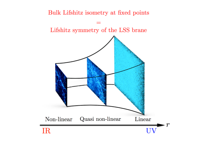
Figure 1: A pictorial representation of our set-up. The six-dimensional bulk enjoys a Lifshitz isometry and realizes the Lifshitz symmetry of the dual field LSS theory on the our universe, the four-dimensional LSS brane, at the fixed points. The flow from large to small $r$ of the bulk dynamical exponent $z$ describes the evolution from the large- to the small-scale LSS. The size of the slices transverse to $r$ are illustrated in comoving coordinates for a fixed physical size.

The paper is organized as follows. In section 2 we describe why the Lifshitz symmetry is an exact symmetry, at any level of perturbation theory, for the dynamics of the dark matter during the matter-dominated period. In section 3 we identify the dynamical exponents of the Lifshitz symmetry for the LSS. In section 4 we describe the gravity dual. In section 5 we discuss the brane cosmology and identify the correct matching between the values of the dynamical exponents at the bulk fixed points with the ones on the LSS brane in section 6. In section 7 we describe the Lifshitz RGE flow of the Lifshitz dynamical exponent and deal with the notion of holographic dark matter in section 8. We conclude in section 9. The paper is also supplemented by Appendix A where we explain how to identify the dual fields.

2 The LSS Lifshitz symmetry

In this section we show that the evolution of dark matter particles in a matter-dominated universe enjoys a Lifshitz symmetry. This is a standard result that goes back to Peebles [25] and can be found in many good cosmology textbooks. We show it here for completeness and to remark that the Lifshitz symmetry is indeed valid at any scale.

Let us define the dark matter (of mass $m$) phase space density $f(\vec{p},\vec{x},\tau)$ in terms of the conformal time $\tau$, the comoving coordinates $\vec{x}$ and the canonical momentum $\vec{p}=am\vec{u}$ defined in terms of the peculiar velocity $\vec{u}$, where $a(\tau)$ is the scale factor of the expansion of the universe with rate ${\cal H}$. The phase space describing the self-gravitating gas of dark matter particles obeys the following Boltzmann equation

$$\frac{\partial}{\partial\tau}f(\vec{p},\vec{x},\tau)+\frac{1}{am}\vec{p}\cdot\vec{\nabla}_{\vec{x}}f(\vec{p},\vec{x},\tau)-am\vec{\nabla}_{\vec{x}}\Phi\cdot\vec{\nabla}_{\vec{p}}f(\vec{p},\vec{x},\tau)=0.$$ (2.1)

In addition, the canonical momentum obeys the relation

$$\frac{{\rm d}\vec{p}}{{\rm d}\tau}=-am\vec{\nabla}_{\vec{x}}\Phi(\vec{x},\tau)$$ (2.2)

and the Newtonian gravitational potential $\Phi(\vec{x},\tau)$ satisfies the Poisson equation

$$\nabla^{2}\Phi(\vec{x},\tau)=4\pi G\,\overline{\rho}\,a^{2}\delta(\vec{x},\tau),\,\,\,\delta(\vec{x},\tau)=\frac{\rho(\vec{x},\tau)-\bar{\rho}}{\bar{\rho}},$$ (2.3)

where $\bar{\rho}$ is the the mean dark matter density. For a matter-dominated universe, the scale factor $a$ scales like $\tau^{2}$ and one can easily verify that Eqs. (2.1), (2.2) and (2.3) are invariant under the Lifshitz symmetry

$$\boxed{\vec{x}^{\prime}=\lambda\vec{x},~{}~{}~{}\tau^{\prime}=\lambda^{\widetilde{z}}\tau}\,,$$ (2.4)

provided that the other quantities are transformed as follows

$$f^{\prime}(\vec{p},\vec{x},\tau) = f(\vec{p}^{\prime},\vec{x}^{\prime},\tau^{\prime}),$$

$$\delta^{\prime}(\vec{x},\tau) = \delta(\vec{x}^{\prime},\tau^{\prime}),$$

$$\vec{p}^{\prime}(\vec{x},\tau) = \lambda^{-(\widetilde{z}+1)}\vec{p}(\vec{x}^{\prime},\tau^{\prime}),$$

$$\Phi^{\prime}(\vec{x},\tau) = \lambda^{2(\widetilde{z}-1)}\Phi(\vec{x}^{\prime},\tau^{\prime}).$$ (2.5)

A few remarks are in order:

• The Lifshitz symmetry is valid only in a matter-dominated universe. When the cosmological constant (or quintessence) dominates and we have to deal with a two-component system, the symmetry is lost. Nevertheless, the Lifshitz symmetry holds with a good approximation also at very small scales, where the dark matter density is much larger than the one provided by the vacuum energy. In this sense, the LSS at highly non-linear scales is Lifshitz symmetric. To get convinced about this point one can think about the spherical collapse model where the scale factor is identified with a local one describing the evolution of a matter-dominated universe with an effective positive curvature and the cosmological constant plays basically no role. Also, matter always largely dominates over the effective curvature term (in particular during the the collapsing phase), only at the turning point the two contributions are equal.

• As we already stressed, the Lifshitz symmetry is present at the level of Boltzmann equation. As such, it is valid on any scale and not only when the fluid approximation of dark matter holds. Even when we look at cosmological scales at which shell crossing and multiple streams occur, the Lifshitz symmetry is there.

• The Lifshitz symmetry is valid for any values of the Lifshitz exponent $\widetilde{z}$.

• One should also keep in mind for the following that the Lifshitz dynamical exponent $\widetilde{z}$ in the four-dimensional system is not going to be identical to the bulk Lifshitz dynamical exponent $z$. This is the reason why we adopt two different notations, $\widetilde{z}$ and $z$, to identify them.

3 The LSS dynamical exponents

In this section we offer some considerations about the values of the Lifshitz dynamical exponents during the LSS evolution. The central quantity in LSS cosmology is the power spectrum of the dark matter perturbations

$$P(k,\tau)=\big{<}\left|\delta_{\vec{k}}(\tau)\right|^{2}\big{>}.$$ (3.1)

For convenience we will define also the dimensionless power spectrum

$$\Delta^{2}(k,\tau)=\frac{k^{3}}{2\pi^{2}}\,P(k).$$ (3.2)

The evolution of the LSS starts with a linear power spectrum $\Delta_{\rm L}^{2}\,\raisebox{-0.43057pt}{${}_{\textstyle<}\atop{}^{\textstyle\sim}$}\,1$ set by the primordial seeds generated during inflation and reprocessed once the perturbations re-enter the horizon. Gravitational instability drives the power spectrum to larger values in the so-called Quasi Non-Linear (QNL) regime where $1\,\raisebox{-0.43057pt}{${}_{\textstyle<}\atop{}^{\textstyle\sim}$}\,\Delta_{\rm QNL}^{2}\,\raisebox{-0.43057pt}{${}_{\textstyle<}\atop{}^{\textstyle\sim}$}\,10^{2}$. During this phase perturbations grow faster than during the linear regime, till they enter in the so-called Non-Linear (NL) regime, $\Delta_{\rm NL}^{2}\,\raisebox{-1.29167pt}{${}_{\textstyle>}\atop{}^{\textstyle\sim}$}\,10^{2}$ when the growth of the perturbations slows down.

If the Lifshitz symmetry holds, the power spectrum must scale like

$$P(k,\tau)\equiv\tau^{3/\widetilde{z}}\mathcal{P}(k\tau^{1/\widetilde{z}}),$$ (3.3)

where $\mathcal{P}$ is a priori an arbitrary (but possibly power-law) function. In the following we will discuss what are the values of the critical Lifshitz exponent characterizing the three different phases. At this stage we do not aim at a precise quantitative determination, but rather we aim at characterizing the qualitative behavior of the critical Lifshitz exponents.

3.1 The linear regime

In the linear regime the power spectrum is characterized by a spectral index $n$ and its growth is parametrized by the following expression

$$P_{\rm L}(k_{\rm L},\tau)\sim\,D^{2}(\tau)k_{\rm L}^{n},$$ (3.4)

where $D(\tau)$ is the linear growth factor. In the matter-dominated period $D(\tau)=a(\tau)\sim\tau^{2}$ and by matching this behavior against the generic expression (3.3), one finds

$$\boxed{\widetilde{z}_{\rm L}=\frac{n+3}{4}}\,.$$ (3.5)

Of course, as soon as the vacuum energy takes over, the Lifshitz symmetry is lost and therefore the value (3.5) should be understood as the initial condition (to be fixed in the matter-dominated period) of the brane Lifshitz dynamical exponent $\widetilde{z}$ which, in turn, identifies the initial condition of the bulk Lifshitz dynamical exponent $z$ in the dual theory.

N-body simulations [18] indicate that the appropriate value for our universe of $\widetilde{z}_{\rm L}$ when $\Delta_{\rm L}^{2}(k)={\cal O}(1)$ is obtained for $n\simeq-1.6$. This leads to $\widetilde{z}_{\rm L}\simeq 1/3$. As we shall see, this value remarkably corresponds in the gravity dual model to a fixed point of the RGE flow where the bulk symmetry is augmented by a non-relativistic conformal symmetry giving rise to the Schrödinger group.

3.2 The quasi non-linear regime

While the analytical methods fail in the QNL and NL regimes, invaluable fitting formulas calibrated by simulations which describe how the power spectra of density fluctuations evolve into the NL regime of hierarchical clustering have been found in a series of remarkable papers [19, 20, 21, 22]. The foundation of these fitting formulas is the so-called HKLM [19] relation which has two parts. The first part is to connect the nonlinear wavenumber to the linear one

$$k_{\rm L}=\left[1+\Delta^{2}_{\rm NL}(k_{\rm NL},\tau)\right]^{1/3}\,k_{\rm NL}.$$ (3.6)

The reasoning behind this is pair conservation. The second part of the HKLM procedure is to conjecture that the nonlinear correlation function is a universal function of the linear one,

$$\Delta^{2}_{\rm NL}(k_{\rm NL},\tau)=f\left[\Delta^{2}_{\rm L}(k_{\rm L},\tau)\right].$$ (3.7)

The asymptotics of the function $f(x)$ can be deduced readily. For small arguments $x\ll 1$, $f(x)\simeq x$. Following the collapse of structures, $f(x)\simeq x^{3/2}$ derived from the hypothesis that although the separation of clusters will alter as the universe expands, their internal density structure will stay constant with time. Numerical experiments interpolated between these two regimes, in a manner that empirically showed negligible dependence on the power spectrum [19, 20, 21, 22].

In the QNL regime we can approximate the expression (3.6) as

$$k_{\rm L}=\left[\Delta^{2}_{\rm QNL}(k_{\rm QNL},\tau)\right]^{1/3}\,k_{\rm QNL}.$$ (3.8)

Furthermore, if we pose $f(x)=x^{1+\alpha}$, with $3.5\,\raisebox{-0.43057pt}{${}_{\textstyle<}\atop{}^{\textstyle\sim}$}\,\alpha\,\raisebox{-0.43057pt}{${}_{\textstyle<}\atop{}^{\textstyle\sim}$}\,4.5$ [20], we have

$$\Delta^{2}_{\rm QNL}(k_{\rm QNL},\tau) \sim D(\tau)^{(6-2\gamma_{\rm QNL})(1+\alpha)/3}\,k_{\rm QNL}^{\gamma_{\rm QNL}},$$

$$\gamma_{\rm QNL} = \frac{3(3+n)(1+\alpha)}{3+(3+n)(1+\alpha)}.$$ (3.9)

Notice that in the QNL regime, the growth of perturbations speeds up. For $\gamma\simeq 1.5$ and $\alpha\simeq 4$, the perturbations scale like $D^{5}$, much faster than what they do on the linear regime.

If we phenomenologically parametrize the linear growth factor as $D(\tau)\sim\tau^{2+\epsilon}$ with a constant $\epsilon>0$ when the vacuum energy dominates, then one can define the QNL dynamical exponent

$$\widetilde{z}_{\rm QNL}=\frac{n+3}{4(1+\epsilon)}.$$ (3.10)

This is a fake dynamical exponent as the Lifshitz symmetry is slightly broken, but the interesting point is that it decreases with respect to the value during the linear phase. We will argue that in the dual theory this corresponds to the running of the bulk Lifshitz dynamical exponent to values larger than the fixed point.

3.3 The non-linear regime

In the NL regime, even when the vacuum energy dominates the effective expansion at small scales is governed by dark matter. Repeating the computations of the previous subsection with $\alpha=1/2$ and assuming that the Lifshitz symmetry holds, one finds

$$\Delta^{2}_{\rm NL}(k_{\rm NL},\tau) \sim \tau^{(6-2\gamma_{\rm NL})}\,k_{\rm NL}^{\gamma_{\rm NL}},$$

$$\gamma_{\rm NL} = \frac{3(3+n)}{5+n}.$$ (3.11)

This corresponds to the value of the dynamical exponent

$$\boxed{\widetilde{z}_{\rm NL}=\frac{n+3}{4}}\,.$$ (3.12)

The fact that this value matches the linear one in Eq. (3.5) is of course obvious because the Boltzmann equation describing the evolution of the dark matter particles at non-linear scales experiences a matter-dominated environment. The value (3.12) should be understood as the final condition of the brane Lifshitz dynamical exponent $\widetilde{z}$ which, in turn, identifies the final condition of the bulk Lifshitz dynamical exponent $z$ in the dual theory.

A satisfactory gravity dual will then possess the following property: if the RGE flow when going from the UV to the IR in the bulk causes the the bulk Lifshitz dynamical exponent to run from a fixed point back to the same fixed point by acquiring different values during the intermediate evolution, this should be reflected in a change of the LSS Lifshitz dynamical exponent from its value at linear scales back to the same value at highly non-linear scales by decreasing its value in the intermediate evolution. We will show in the following that such a gravity dual can indeed be constructed.

4 The LSS gravity dual

Having identified the critical Lifshitz exponents for the LSS, we now proceed to construct the gravity dual theory possessing the appropriate Lifshitz symmetry. As we already mentioned in the introduction, the following metric

$${\rm d}s^{2}=-\frac{L^{2z}}{r^{2z}}{\rm d}t^{2}+\frac{L^{2}}{r^{2}}\left(2{\rm d}t{\rm d}\xi+{\rm d}\vec{x}^{2}+{\rm d}r^{2}\right)$$ (4.1)

is Lifshitz symmetric. In particular, it is symmetric under the scaling

$$t\to\lambda^{z}t,~{}~{}~{}r\to\lambda r,~{}~{}~{}\vec{x}\to\lambda\vec{x},~{}~{}~{}\xi\to\lambda^{2-z}\xi.$$ (4.2)

In fact, the metric (4.1) has more symmtries. It is invariant under an eleven-dimensional group of isometries consisting of translations in $\vec{x}$ and $t$, rotations of $\vec{x}$, Lifshitz transformations, and Galilean boosts

$$t\to t^{\prime}=t,\,\,\vec{x}\to\vec{x}^{\prime}=\vec{x}-\vec{v}t,\,\,\xi\to\xi^{\prime}=\xi+\frac{1}{2}\left(2\vec{v}\cdot\vec{x}-v^{2}t\right).$$ (4.3)

What is important to notice is that $z=2$ is a point of enhanced symmetry. Indeed for such a value, there is an additional special conformal isometry

$$t\to t^{\prime}=\frac{t}{1+\alpha t},\,\,\vec{x}\to\vec{x}^{\prime}=\frac{\vec{x}}{1+\alpha t},\,\,r\to r^{\prime}=\frac{r}{1+\alpha t},\,\,\xi\to\xi^{\prime}=\xi+\frac{\alpha}{2}\frac{x^{2}+r^{2}}{1+\alpha t}.$$ (4.4)

This special conformal symmetry together with the symmetries above form the Schrödinger group [24]. This point will be come relevant in the following as we shall show that the LSS dynamical exponent for our observed universe at linear and non-linear scales corresponds to a bulk dynamical exponent $z$ intriguingly close to the point of enhanced symmetry.

From the metric (4.1) one can identify what the running of $r$ corresponds to in terms of the physical length scales on a brane located at a given $r$: being $g_{ij}=(L^{2}/r^{2})\delta_{ij}$, we read that the “redshift” factor scales like $1/r$. This implies that that a brane observer at some reference scale $r_{*}$ will determine a physical length as $\ell_{*}=(L_{*}/r_{*})\ell_{\rm com}$. At another point $r=R(t)$, the same mode will look having a different $\ell=(L/R)\ell_{\rm com}$. Therefore, we get that

$$\boxed{\ell=\frac{r_{*}}{R(t)}\ell_{*}}\,.$$ (4.5)

If our universe is then identified with a moving brane with posotion $R(t)$ in the bulk, going from large to small values of $r$ corresponds to go from UV to the IR part in the bulk. In section 5 we will show that $R(t)$ will correspond with the inverse of the induced scale factor on the brane when the universe is matter-dominated.

The metric (4.1) is the solution of a massive Maxwell field coupled to AdS gravity [14, 15]. Indeed, let us consider the action

$$S=\int{\rm d}^{6}x\sqrt{-g}\left(R-2\Lambda-\frac{1}{4}F_{\mu\nu}F^{\mu\nu}+\frac{1}{2}m^{2}A_{\mu}A^{\mu}\right).$$ (4.6)

The equation for the massive vector $A_{\mu}$ is

$$\partial_{\nu}\left(\sqrt{-g}g^{\nu\rho}g^{\mu\sigma}F_{\rho\sigma}\right)-m^{2}\sqrt{-g}g^{\mu\nu}A_{\nu}=0~{}.$$ (4.7)

Symmetry considerations lead one to look for solutions for the gauge field of the type

$$A_{\mu}=A_{0}(r)\delta^{0}_{\mu}.$$ (4.8)

The field Eq. (4.7) imposes

$$A_{0}=\frac{\rho_{0}}{z(z+3)}\frac{1}{r^{z}},$$ (4.9)

where $\rho_{0}$ is constant if we choose

$$m^{2}=\frac{1}{L^{2}}\left[z(z+3)\right].$$ (4.10)

Let us note that the above relation is invariant under

$$z\to-z-3.$$ (4.11)

The constant $\rho_{0}$ can be specified by Einstein equations. It turns out that for the metric (4.1) we have the following components of the Einstein tensor

$$G_{00}=(-13+z+2z^{2})\frac{1}{L^{2}}\frac{L^{2z}}{r^{2z}},\qquad G_{0\xi}=G_{xx}=G_{yy}=G_{zz}=G_{rr}=\frac{10}{r^{2}}.$$ (4.12)

This implies that the energy-momentum tensor must take the form [14, 15]

$$T_{\mu\nu}=-\Lambda g_{\mu\nu}-{\mathcal{E}}\delta_{\mu}^{0}\delta_{\nu}^{0}g_{00},$$ (4.13)

with

$$\Lambda=-\frac{1}{L^{2}},~{}~{}~{}{\mathcal{E}}=\frac{2z^{2}+z-3}{L^{2}}.$$ (4.14)

We can compare this with the energy-momentum tensor of the vector field

$$T^{\mu\nu}=F^{\mu\beta}F^{\nu}_{\beta}-\frac{1}{4}g^{\mu\nu}F_{\alpha\beta}F^{\alpha\beta}-m^{2}A^{\mu}A^{\nu}+\frac{1}{2}g^{\mu\nu}m^{2}A_{\rho}A^{\rho}~{},$$ (4.15)

which, for the field in Eq. (4.9) matches (4.13) if the constant $\rho_{0}$ is

$$\rho_{0}^{2}={\mathcal{E}}\frac{2z(z+3)^{2}}{2z+3}L^{2z+2}=2z(z-1)(3+z)^{2}L^{2z}.$$ (4.16)

Having constructed the appropriate gravity dual enjoying the Lifshitz symmetry (1.1), we now study the four-dimensional brane cosmological and matching between the brane and bulk Lifshitz dynamical exponents. We will then proceed to show that our gravitational dual of Lifshitz-like theories come with the relevant perturbations that induce the flow of the dynamical exponent towards a fixed point. This flow is reflected in the evolution of the brane Lifshitz dynamical exponent from the initial condition $\widetilde{z}_{\rm L}$ for the linear perturbations down to the final fixed point value $\widetilde{z}_{\rm NL}$ on small scales passing through $\widetilde{z}_{\rm QNL}$ under the action of the relevant operator represented by the four-dimensional cosmological constant. In other terms, the bulk flow accounts for the small breaking of the Lifshitz symmetry during the phase in which the universe is dominated by the vacuum energy till the dynamical exponent flows into a fixed point on very small scales.

5 Brane Cosmology

Let us now consider a four-brane floating around in the background (4.1) whose motion will induce a cosmological evolution on the branes [26, 27]. According to the standard nomenclature, a four-brane is a five-dimensional hypersurface embedded here in the six-dimensional background. The coordinates of the four-brane are then $(\zeta^{0},\zeta^{i},\zeta^{4})~{}(i=1,2,3)$ and let us assume that its position in the gauge $(\zeta^{0}=t,\zeta^{i}=x^{i},\zeta^{4}=\xi)$ is at $r=R(t)$. In other words, the four-brane moves perpendicular to the $r$-direction. In this case, for a generic metric of the form

$${\rm d}s^{2}=-f(r){\rm d}t^{2}+g(r)\left(2{\rm d}t{\rm d}\xi+{\rm d}\vec{x}^{2}\right)+h(r){\rm d}r^{2},$$ (5.1)

the brane velocity is $u^{\mu}$ (normalized to $u^{\mu}u_{\mu}=-1$) is given by

$$u^{t}=\left(\frac{h\dot{R}^{2}}{f}+\frac{1}{f}\right)^{1/2},~{}~{}~{}u^{r}=\dot{R}.$$ (5.2)

The induced metric on the brane is

$${\rm d}s^{2}_{\rm ind}=-{\rm d}\eta^{2}+g(R(\eta))\left(2\frac{{\rm d}\eta}{f^{1/2}(R(\eta))}{\rm d}\xi+{\rm d}\vec{x}^{2}\right),$$ (5.3)

and $\dot{R}={\rm d}R/{\rm d}\eta$. The normal to the brane satisfies the equation $n^{\mu}u_{\mu}=0$ and it is turns out to be

$$n^{t}=-\sqrt{\frac{h}{f}}u^{r},~{}~{}~{}n^{r}=-\sqrt{\frac{f}{h}}u^{t}.$$ (5.4)

The extrinsic curvature is given by

$$K_{\mu\nu}=\nabla_{\mu}n_{\nu}$$ (5.5)

and the Israel matching condition is

$$K^{+}_{\mu\nu}-K^{-}_{\mu\nu}=-\frac{1}{M_{*}^{4}}\left(T_{\mu\nu}-\frac{1}{4}T^{\lambda}_{\lambda}\gamma_{\mu\nu}\right),$$ (5.6)

where $K^{\pm}_{\mu\nu}$ is the extrinsic curvature left and right of the brane, $T_{\mu\nu}$ is the energy-momentum tensor on the brane, $\gamma_{\mu\nu}$ is the induced metric and $M_{*}$ is the six-dimensional Planck mass. The extrinsic curvature for the metric (5.1) is found to be

$$K^{\pm}_{\mu\nu}=\mp\left(\frac{1}{h_{\pm}}+\dot{R}^{2}\right)^{1/2}\frac{g^{\prime}}{2g}.$$ (5.7)

In addition, a four-brane with tension $\sigma$ and a perfect fluid on its five-dimensional world-volume with energy density $\rho_{5}$ and pressure $P_{5}$ the energy-momentum tensor is

$$T_{\mu\nu}=-\sigma\gamma_{\mu\nu}+\rho_{5}U_{\mu}U_{\nu}+P_{5}\left(\gamma_{\mu\nu}+U_{\mu}U_{\nu}\right).$$ (5.8)

Hence, Eq. (5.6) is explicitly written as

$$\left(\frac{1}{h_{+}}+\dot{R}^{2}\right)^{1/2}+\left(\frac{1}{h_{-}}+\dot{R}^{2}\right)^{1/2}=\frac{1}{4M_{*}^{4}}(\sigma+\rho_{5})\frac{2g}{g^{\prime}}.$$ (5.9)

For a Lifshitz background

$$f_{\pm}=\frac{L^{2z_{\pm}}}{r^{2z_{\pm}}}\,,~{}~{}~{}~{}g_{\pm}=h_{\pm}=\frac{L^{2}}{r^{2}}.$$ (5.10)

In the particular case $z_{+}=z_{-}$, we find that

$$\dot{R}^{2}=-\frac{R^{2}}{L^{2}}+\frac{R^{2}}{64M_{*}^{8}}(\rho_{5}+\sigma)^{2}.$$ (5.11)

We may write this equation as a Friedmann equation after we identify the scale factor and recall that we need to perform a further Kaluza-Klein along the $\xi$-direction. As it is usual in the Kaluza-Klein set-up, the induced metric in Eq. (5.3) is not in the appropriate Einstein frame and some redefinition is needed. The five dimensional action is

$${\cal S}=\int{\rm d}^{3}x{\rm d\xi}{\rm d}\eta\,\sqrt{-g_{\rm ind}}\,{\cal L}_{\rm eff}^{(5)},$$ (5.12)

where

$$\sqrt{-g_{\rm ind}}=\left(\frac{R}{L}\right)^{z-5}.$$ (5.13)

Defining a four-dimensional effective action

$${\cal L}_{\rm eff}^{(4)}=\int{\rm d}\xi\,{\cal L}_{\rm eff}^{(5)},$$ (5.14)

we get that

$${\cal S}=\int{\rm d}^{3}x{\rm d}\eta\left(\frac{R}{L}\right)^{z-5}\,{\cal L}_{\rm eff}^{(4)}=\int{\rm d}^{3}x{\rm d}\eta\,\sqrt{-g_{\rm E}}\,{\cal L}_{\rm eff}^{(4)}.$$ (5.15)

Therefore, the four-dimensional action can be reproduced through a four-dimensional Einstein metric

$${\rm d}s^{2}_{\rm E}=-\left(\frac{R}{L}\right)^{2z-4}{\rm d}\eta^{2}+\left(\frac{L}{R}\right)^{2}{\rm d}\vec{x}^{2}.$$ (5.16)

We can write Eq. (5.16) as

$${\rm d}s^{2}_{\rm E}=\left(\frac{L}{R}\right)^{2}\bigg{[}-\left(\frac{R}{L}\right)^{2z-2}{\rm d}\eta^{2}+{\rm d}\vec{x}^{2}\bigg{]}=a^{2}(\tau)\left(-{\rm d}\tau^{2}+{\rm d}\vec{x}^{2}\right),$$ (5.17)

where we have defined the four-dimensional scale factor

$$a=\frac{L}{R},$$ (5.18)

and the conformal time through the relation

$${\rm d}\tau=a^{1-z}{\rm d}\eta.$$ (5.19)

Eq. (5.11) takes the form

$$\left(\frac{\dot{a}}{a}\right)^{2}=-\frac{1}{L^{2}}+\frac{1}{64M_{*}^{8}}(\rho_{5}+\sigma)^{2}.$$ (5.20)

For the particular case of

$$\sigma=\frac{8M_{*}^{4}}{L},$$ (5.21)

we get the Friedmann equation five-dimensional (expressed in terms of the four-dimensional scale factor)

$$\left(\frac{\dot{a}}{a}\right)^{2}=\frac{1}{4M_{*}^{4}L}\,\rho_{5}+\frac{1}{64M_{*}^{8}}\rho_{5}^{2}\,.$$ (5.22)

Note that $\rho_{5}$ is the five-dimensional energy density. We may assume that the extra fifth coordinate is a KK compact direction with radius $R_{5}$. In that case, the zero-mode reduced four-dimesional energy density $\rho$ will be given by

$$\rho=2\pi R_{5}\rho_{5}.$$ (5.23)

Therefore, to leading order in $1/R_{5}^{2}$ we will have

$$\left(\frac{\dot{a}}{a}\right)^{2}=\frac{8\pi G_{\rm N}}{3}\rho,$$ (5.24)

where

$$8\pi G_{N}=\frac{3}{12\pi LR_{5}M_{*}^{4}}.$$ (5.25)

Therefore, the standard FRW dynamics is recovered on the brane for the four-dimensional zero-modes of the five-dimensional KK brane at $r=R(\tau)$. At this stage, let us remark that the four-dimensional brane cosmology has been obtained by adding an extra-dimensional source of energy $\rho_{5}$ with the appropriate scaling of the scale factor to achieve the correct four-dimensional universe evolution. While this is the standard procedure in the literature and is perfectly legitimate, it would be desirable to realize the dark matter on the brane by slightly altering the bulk geometry in such a way that the dark matter on the brane inherits the symmetry properties of the bulk. We will come back to this point later on.

6 The correspondance between the bulk and the brane Lifshitz dynamical exponents

The next step is to find the correspondance between the brane dynamical exponent $\widetilde{z}$ and the bulk dynamical exponent $z$. To do so, we express the coordinate time $\eta$, which is invariant under Lifshitz scaling, in terms of the conformal time $\tau$, which scales as in Eq. (2.4). First of all, going back to Eq. (4.5), we see that the running of $r$, identified with the movement of the LSS brane in the bulk, corresponds to a change of the physical length according to the relation

$$\ell(t)=\frac{a(t)}{a_{*}}\ell_{*}.$$ (6.1)

For the matter-dominated period which is of interest for us, $a(\tau)\sim\tau^{2}$ and using Eq. (5.19) we get

$$\eta\sim\tau^{2z-1}.$$ (6.2)

Therefore, recalling that $\eta$ is invariant and that $\tau$ transforms into $\lambda^{\widetilde{z}}\tau$, we find

$$\widetilde{z}=\frac{1}{2z-1}.$$ (6.3)

As we have previously noticed, the point $z=2$ is a point of enhanced symmetry. At this point, the value of $\widetilde{z}$ turns out to be $\widetilde{z}=1/3$

$$\boxed{{\rm Bulk}\,\,{\rm enhanced}\,\,{\rm symmetry}\,\,{\rm point}\,\,z=2\,\,\Rightarrow\,\,\widetilde{z}=\frac{1}{3}\,\,{\rm on}\,\,{\rm the}\,\,{\rm brane}\,\,\Rightarrow\,\,n=-1.6}\,.$$ (6.4)

This is one of the main results of the paper and quite exciting because this value of the LSS dynamical exponent $\widetilde{z}=(n+3)/4$ is obtained exactly for the spectral index $n=-1.6$, which is approximately the value of the spectral index for our observed universe when $\Delta^{2}_{\rm L}$ becomes of order unity.

In the approximation of a pure matter-dominated universe, the so-called Einstein-de Sitter universe, the dynamical Lifshitz exponents, both on the brane and in the bulk, are constant and the description of the LSS through a gravity dual with the full Schrödinger symmetry might represent a suitable starting point to characterize the dark matter perturbations.

7 Lifshitz flows of the dynamical exponent

Having constructed the gravity dual possessing the Lifshitz isometry and having identified the mapping between the Lifshitz bulk dynamical exponent with the one on the four-dimensional brane, we now study the renormalization group flow between fixed points. This flow is supposed to capture the departure from the exact Lifshitz symmetry which occurs when the universe is not matter-dominated. In the dual theory the variable $r$ goes from an UV initial condition at large $r$, identified with the Lifshitz fixed-point when the linear perturbations are in the matter-dominated period, to an IR Lifshitz fixed-point at small $r$.

A simple Langrangian which is sufficiently general to capture the flow is the one where the latter is triggered and controlled by a scalar field $\phi$ with potential $V(\phi)$ and coupling $W(\phi)$ to the gauge field

$${\cal S}=\int{\rm d}^{6}x\sqrt{-g}\bigg{(}R-2V(\phi)-\frac{1}{2}(\partial\phi)^{2}-\frac{1}{4}F_{\mu\nu}F^{\mu\nu}-\frac{1}{2}W(\phi)A_{\mu}A^{\mu}\bigg{)}.$$ (7.1)

A metric ansatz which is sufficiently general to capture this flow is

$${\rm d}s^{2}=-e^{2A(y)}{\rm d}t^{2}+e^{2B(y)}\Big{(}2{\rm d}t{\rm d}\xi+{\rm d}\vec{x}^{2}\Big{)}+{\rm d}y^{2}$$ (7.2)

and in addition

$$\phi=\phi(y),~{}~{}~{}A_{\mu}=H(y)e^{A(y)}\delta_{\mu}^{0}.$$ (7.3)

The coordinate $y$ above is related to $r$ defined in Eq. (4.1) as

$${\rm d}r^{2}=e^{-2B(y)}{\rm d}y^{2}.$$ (7.4)

The equations of motion can be expressed in terms of the scalars $\phi(y)$, $H(y)$ and

$$L(y)=\frac{1}{B^{\prime}(y)},~{}~{}~{}z(y)=\frac{A^{\prime}(y)}{B^{\prime}(y)},$$ (7.5)

(where prime denotes derivative with respect to $y$) as

$$0 = \frac{z^{\prime}L-L^{\prime}z}{L^{2}}H+\frac{z^{2}}{L^{2}}H+\frac{2z}{L}H^{\prime}+\frac{3}{L}\Big{(}H^{\prime}+\frac{z}{L}H\Big{)}+H^{\prime\prime}-WH,$$ (7.6)

$$0 = \phi^{\prime\prime}+\frac{5}{L}\phi^{\prime}-2\partial_{\phi}V,$$ (7.7)

$$0 = z^{\prime}L+(1-z)L^{\prime}+(3+2z)(z-1)-\frac{1}{2}L^{2}\Big{[}\left(H^{\prime}+\frac{z}{L}H\right)^{2}+WH^{2}\Big{]},$$ (7.8)

$$0 = \frac{1}{2}\phi^{\prime 2}-\frac{4}{L^{2}}L^{\prime},$$ (7.9)

$$0 = \frac{1}{4}\phi^{\prime 2}-V-\frac{10}{L^{2}}.$$ (7.10)

It is easy to check that for the particular case

$$W=\frac{z_{0}(z_{0}+3)}{L_{0}^{2}},~{}~{}~{}V=-\frac{10}{L_{0}^{2}},~{}~{}~{}\partial_{\phi}V(\phi_{0})=0,~{}~{}~{}L=L_{0},$$ (7.11)

the solution is

$$A=\frac{z_{0}y}{L_{0}},~{}~{}~{}B=\frac{y}{L_{0}},~{}~{}~{}\phi=\phi_{0},~{}~{}~{}H=\sqrt{\frac{2(z_{0}-1)}{z_{0}}},$$ (7.12)

which is just Eq. (4.1). The system of Eqs. from (7.6) to (7.10) has four fixed points at [33, 34]

$$H = 0,\,\,z=-\frac{3}{2},$$

$$H = 0,\,\,z=1,$$

$$H^{2} = \frac{1}{L^{2}W}\bigg{(}2L^{2}W-3-\sqrt{9+4L^{2}W}\bigg{)},\,\,z=-\frac{3}{2}\bigg{(}1-\sqrt{1+\frac{4L^{2}W}{9}}\bigg{)},$$

$$H^{2} = \frac{1}{L^{2}W}\bigg{(}2L^{2}W-3+\sqrt{9+4L^{2}W}\bigg{)},\,\,z=-\frac{3}{2}\bigg{(}1+\sqrt{1+\frac{4L^{2}W}{9}}\bigg{)}.$$ (7.13)

It can easily be checked that for the forth fixed point

$$W\geq 0,~{}~{}z\leq-3,~{}H^{2}\geq 0.$$ (7.14)

What is more relevant for us is the third fixed point for which

$$W\geq\frac{4}{L^{2}},~{}~{}~{}z\geq 1,~{}H^{2}\geq 0.$$ (7.15)

Some comments are in order:

• For $L^{2}W=10$, the fixed point is at $z=2$, corresponding to $H^{2}=1$. As we already remarked, this point is particularly interesting because is not only a point of enhanced symmetry in the bulk, but it also corresponds to the dynamical Lifshitz exponent on the brane favoured for our observed universe and obtained for a spectral index $n\simeq-1.6$.

• In a Einstein-de Sitter universe always dominated by dark matter, studied for instance in Ref. [31], the brane dynamical Lifshitz exponent remains constant, say $\widetilde{z}=1/3$ for $z=2$. This is trivially reproduced in our set-up taking the gauge field configuration $H^{2}=1$ along all the RGE flow.

• Values of $n$ different, but in any case in the vicinity of $n=-1.6$, correspond to values of the bulk dynamical exponent $z$ slightly different from $z=2$. Nevertheless all these points with $z\neq 2$ are fixed points of the RGE flow. Therefore, all of them could be used for cosmological considerations on the LSS. The price to pay, maybe not that expensive, would be that these points are not points of enhanced symmetry.

For the running among generic fixed points where the gauge field is not zero, the gauge dynamics is important and the full system of equations Eqs. (7.6)-(7.10) should be considered. In particular, we are interested in the RGE flow going from $z=2$ and back to $z=2$. This corresponds on the brane to the flow of the dynamical exponent $\widetilde{z}$ from linear to highly non-linear scales.

To find an example of such a flow we follow Ref. [34] and we write the potential for the scalar field as

$$V(\phi)=V_{0}+V_{1}\phi+\frac{1}{2}V_{2}\phi^{2}+\frac{1}{6}V_{3}\phi^{3}+\frac{1}{24}V_{4}\phi^{2}(\phi-\phi_{0})^{2},$$ (7.16)

and similarly for the function

$$W(\phi)=W_{0}+W_{1}\phi+\frac{1}{2}W_{2}\phi^{2}+\frac{1}{6}W_{3}\phi^{3}.$$ (7.17)

Assuming a flow from $\phi=0$ to $\phi=\phi_{0}$ and taking the first derivative of $W(\phi)$ to vanish at the fixed points, the set of conditions can be chosen as

$$V_{0} = -\frac{10}{L_{\rm IR}^{2}}=-W_{0},$$

$$V_{1} = 0=W_{0},$$

$$V_{2}\phi_{0}^{2} = -60\left(\frac{1}{L_{\rm UV}^{2}}-\frac{1}{L_{\rm IR}^{2}}\right)=-W_{2}\phi_{0}^{2},$$

$$V_{3}\phi_{0}^{3} = 120\left(\frac{1}{L_{\rm UV}^{2}}-\frac{1}{L_{\rm IR}^{2}}\right)=-W_{3}\phi_{0}^{3}.$$ (7.18)

The solution of the system cannot be found in closed form. However, its form is given in Fig. 2 for some choice of the parameters. In this example $z$ runs from $z=2$ back to $z=2$ (and correspondingly $\widetilde{z}$ runs from $\widetilde{z}=1/3$ back to $\widetilde{z}=1/3$) from the the UV to the IR (that is at larger and larger values of the scale factor). This running therefore catches the behavior of the LSS dynamical exponent from the linear to the NL phase passing through the QNL stage, when indeed $\widetilde{z}$ is smaller and perturbations runs faster in time.

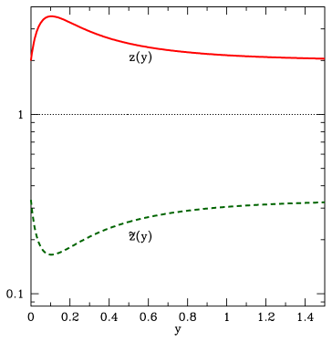
Figure 2: A possible example of the evolution of the exponents $z$ and $\widetilde{z}$ as a function of the coordinate $y$. They run from $z=2$ and $\widetilde{z}=1/3$ to the same values. These two regions correspond to linear and non-linear regimes. The values are taken to be $L_{0}=1$, $L_{\rm UV}=11L_{0}/10$, $V_{0}=-W_{0}=-10$, $V_{1}=-W_{1}=0$, $V_{2}=-W_{2}=-60(1/L_{\rm UV}^{2}-1)$, $V_{3}=-W_{3}=120(1/L_{\rm UV}^{2}-1)$, $V_{4}=24/\phi_{0}^{2}$, $\phi_{0}=1$.

This running of the dynamical exponent $z$ in the bulk, corresponding to changes of the dynamical exponent $\widetilde{z}$, in Fig. 2 is of course only exemplary. A more realistic one should reproduce real data.

In the example above we have assumed that the dark matter on the brane is provided by a dominant source given by the projected five-dimensional energy density $\rho_{5}$. In the following we elaborate about relaxing this option and realizing the dark matter on the brane in terms of a dual field in the bulk, in such a way that the symmetry properties of the bulk is inherited on the brane.

8 Holographic dark matter

Comparing with the brane-world holography in the usual Randall-Sundrum setup [35], it is well known that the symmetries of AdS space allows for a radiation fluid on the brane, a relativistic analogue of our $\rho_{5}$ above. This radiation dominated brane-world cosmology can however be understood from a holographic point of view, where instead of a radiation fluid added by hand on the brane, a black hole is added in the bulk, and the emergent radiation dominated universe on the brane is purely a higher dimensional geometric effect due to a black hole in the bulk. It is believed that a dual CFT, slightly broken by the brane location, describes the “dark radiation” on the brane, and a bulk-brane duality exists [36, 37, 38]. Heuristically, one can think that it is the Hawking radiation of the bulk black hole that is heating the brane.

Similarly it would be desirable if we could set $\rho_{5}=0$, and realize dark matter on the brane by slightly altering the bulk geometry instead. In this way, if the dark matter on the brane is realized in terms of a dual field in the bulk, we expect that the fluid on the brane inherits the symmetry properties of the bulk.

In fact, it is clear that if the bulk geometry is altered in such a way that $L=L(R)$ and $L(R)$ has the right functional form, the geometry will lead to an ”optical illusion” of “dark matter” on the brane. The holographic dual of dark matter, which will give the correct function form of $L(R)$, will be in our set-up simply the scalar field $\phi$ in the bulk we encountered in the previous section to cause the running of the bulk dynamical exponent plus a ghost-like field $\theta$. The addition of these scalar fields leading to dark matter on the brane is of course a perturbation of the system from the Lifshitz invariant fixed point, but again it is an irrelevant perturbation and the system will flow immediately back towards the fixed point.

Let us therefore investigate the issue of the holographic dark matter and explore further the Friedmann equation in Eq. (5.20). We will assume $\rho_{5}=0$, so that the brane has only tension $\sigma$. Let us first provide some general considerations. The function $L(R)$ has to decrease when going from the UV to the IR (in other words from smaller to larger values of the scale factor). From now on we take the variable $y$ to be positive.

We write the asymptotic behavior of the function $L(y)$ as

$$L(y)\simeq A+De^{-Cy},\,\,\,C>0,$$ (8.1)

when $y\to+\infty$. Therefore

$$\frac{1}{L^{2}}\simeq\frac{1}{A^{2}}\left(1-2\frac{D}{A}e^{-Cy}\right).$$ (8.2)

The function $B(y)$ is such that $B^{\prime}(y)=1/L(y)$ and therefore we get

$$B\simeq\frac{y}{A}.$$ (8.3)

Because of Eq. (5.18), we know that the scale factor is related to the function $B(y)$ as $a=e^{B}$. This means that for $y\to+\infty$ we have $a=e^{B}=e^{y/A}$ and

$$-\frac{1}{L^{2}}\simeq-\frac{1}{A^{2}}\left(1-2\frac{D}{A}a^{-CA}\right).$$ (8.4)

From this expression we infer

$$C\cdot A=+3\Rightarrow A>0,\,\,\,\,\,D>0\,\,\,{\rm for}\,\,\,y\to+\infty.$$ (8.5)

In other words, in order to reproduce the correct Friedmann equation the function $L(y)$ needs to reach a positive asymptote at $y\to+\infty$ from above. This means that around the asymptotes the function $L(y)$ is decreasing, as it should. This is not consistent with Eq. (7.9)

$$(\phi^{\prime})^{2}=8\frac{L^{\prime}}{L^{2}}>0.$$ (8.6)

So, the behaviour of $L(y)$ is not consistent with the holographic $c$-theorem [33] stating that $L^{\prime}$ has to be positive. In order to bypass this problem, we need to consider a scalar field with the wrong-sign kinetic term. The full action becomes

$${\cal S} = \int{\rm d}^{6}x\sqrt{-g}\bigg{(}R-2V(\phi)-\frac{1}{2}(\partial\phi)^{2}-\frac{1}{4}F_{\mu\nu}F^{\mu\nu}-\frac{1}{2}W(\phi)A_{\mu}A^{\mu}$$ (8.7)

$$+ \frac{1}{2}(\partial\theta)^{2}-2U(\theta)\bigg{)}.$$

All field equations are the same as before, but the following

$$0 = \phi^{\prime 2}-\theta^{\prime 2}-\frac{8}{L^{2}}L^{\prime},$$ (8.8)

$$0 = \frac{1}{4}\phi^{\prime 2}-\frac{1}{4}\theta^{\prime 2}-V-U-\frac{10}{L^{2}},$$ (8.9)

$$0 = \theta^{\prime\prime}+\frac{5}{L}\theta^{\prime}+2\partial_{\theta}U.$$ (8.10)

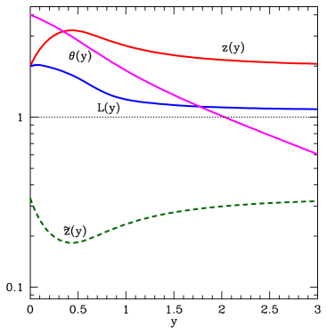
Figure 3: A possible example of the evolution of the exponents $z$, $\widetilde{z}$ and $L(y)$ as a function of the coordinate $y$. They run from $z=2$ and $\widetilde{z}=1/3$ to the same values and $L(y)$ has the correct behaviour to mimic the dark matter. The values are like in Fig. 2, apart from $L_{0}=2$.

Again, analytical solutions are not available, but we show an example in Fig. 3, where we have taken the potential for the ghost field $\theta$ to be $U(\theta)=2/L_{0}^{2}\,\theta^{2}$. In particular, we see that the effect of the wrong-sign in the kinetic term of the $\theta$ field makes the function $L(y)$ to decrease, as needed to reproduce the correct cosmology if we take $\rho_{5}=0$. In this case, taking

$$\frac{1}{A^{2}}=\frac{1}{64M_{*}^{8}\sigma^{2}}+\Lambda_{\rm obs},\,\,\,2\frac{D}{A^{3}}=\frac{8\pi G_{\rm N}}{3},$$ (8.11)

we can reproduce the usual Friedmann equation with a tiny cosmological constant $\Lambda_{\rm obs}$ plus non-relativistic dark matter. Of course, using a ghost scalar field might not be particularly appealing to some reader, but this seems to be the price to pay when abandoning the more standard beaten path of populating the brane with dark matter from a five-dimensional $\rho_{5}$. On the other end, it would be interesting to further investigate the possible relation between the wrong-sign kinetic term of the field $\theta$ with the phenomenon of the gravitational instability on the brane.

9 Criticisms, perspectives and conclusions

In this paper we have taken the first step towards the construction of a gravity dual of the LSS dynamics of our universe. Our considerations are based on the realization that such dynamics respects a Lifshitz symmetry which may manifest itself as an isometry in a six-dimensional bulk where our universe is located as a four-dimensional brane.

We have shown that the $z=2$ value of the bulk Lifshitz dynamical exponent is matched during a matter-dominated period into a brane Lifshitz dynamical exponent which corresponds to the value observed in our universe. This is interesting as $z=2$ is a point of enhanced symmetry. Furthermore, the holographic dynamical exponent in the dual theory can perform an RGE flow between Lifshitz fixed points, going for instance from $z=2$ back to $z=2$. We find it encouraging that the corresponding value of the dynamical exponent on the boundary theory describes the LSS of our observed universe at large and small scales, while deviating in between. This RGE flow of the bulk dynamical exponent is reflected in a growth of the LSS in the non-linear regime with roughly the same rate it has in the the linear regime, but much slower than in the quasi non-linear regime, something that is also observed in current data.

Let us now stress what are (some of) the incomplete aspects of our work:

• We have focussed more on the qualitative aspects of the construction of the gravity dual to show that the RGE flow of the bulk dynamical exponent can explain the running of the brane dynamical exponent observed in our universe. Ultimately, we will have to deal with the more quantitative aspects of the problem.

• A basic point of any gravity dual correspondence is to associate a field in the bulk with the appropriate operator on the boundary. While we elaborate on this step in appendix A, the ultimate goal will be to compute the boundary correlators, for instance of the dark matter density contrast, by solving the bulk gravity equations of motion with the appropriate boundary conditions. This will provide us with the boundary correlators although in a flat background. In order to get the correlators in a curved background, one has to let the brane move, thus producing the cosmological expansion in its world volume. At present, the correspondence we have put forward is at a pure level of a conjecture and we leave these steps for future work.

• Related to the previous point, at this stage we are not able to make any prediction about the correlators, for instance, the power spectrum, of the dark matter on small scales.

• A final point concerns the dual CFT of the gravitational theory we discussed here (and in fact for all gravity duals describing low-energy condensed matter theories). It should be stressed that the background Lifshitz spacetime is not asymptotically locally AdS and one cannot trivially extend standard holographic results in this case. For the particular case of a five-dimensional Schrödinger spacetime, it has been noted already in Ref. [14] that a holographic dual should exists as the Schrödinger spacetime can be obtained by a irrelevant deformation of AdS₅ [32]. Moreover, it was argued in Ref. [30] that the dual theory in this case is a null dipole theory, based on the fact that the Schrödinger spacetime can be obtained from AdS₅ via TsT transformations. Similarly we expect that the dual theory of the six-dimensional Schrödinger spacetime we employed here to be related to the AdS₆ vacuum of massive IIA theory via a chain of dualities and singular boosts. The dual theory is expected to be a null dipole theory, arising from a null dipole deformation of a 5D large $N$ SYM theory in this case as well.

It is clear that the next task will be to establish this conjecture on a firmer footing and use it to explore structure formation in the non-linear regime. We leave it for future work. If successful, an unknown area in the analytical understanding of LSS formation will be charted. In any case, the set-up provides an interesting new arena for testing the limitations of holography and gravitational duals as a tool of studying strongly coupled field theories.

Appendix A Identifying dual fields

As we already remarked, the final goal of any gravity dual of the LSS is to find the dynamics of the relevant boundary observables defined by the theory in the bulk and to construct boundary correlators (such as the one for the density contrast) as given by the value of the renormalized bulk action for specified boundary values of the bulk fields in the Lifshitz backgrounds [14, 15, 16, 17, 39, 40, 41, 42, 43, 44, 45, 46]. In this appendix we take a first step by identifying which the bulk dual fields corresponds to the boundary fields.

A convenient way for our purposes is to perturb the coordinate basis ${\rm d}x^{M}$ according to

$${\rm d}x^{M}\to{\rm d}x^{M}+{h^{M}}_{N}\,{\rm d}x^{N},$$ (A.1)

in such a way that the null structure of spacetime is preserved, that is $\partial_{\xi}$ remains a null vector. Then, the possible perturbations are

$${\rm d}t \to {\rm d}t+{h^{0}}_{0}{\rm d}t+{h^{0}}_{i}\,{\rm d}x^{i},$$

$${\rm d}\xi \to {\rm d}\xi+{h^{\xi}}_{0}\,{\rm d}t+{h^{\xi}}_{\xi}\,{\rm d}\xi+{h^{\xi}}_{i}\,{\rm d}x^{i},$$

$${\rm d}x^{i} \to {\rm d}x^{i}+{h^{i}}_{0}\,{\rm d}t+{h^{i}}_{j}\,{\rm d}x^{j}.$$ (A.2)

The above change in the coordinate basis, give rise to a corresponding metric perturbation

$${\rm d}s^{2} = -\frac{L^{2z}}{r^{2z}}\Big{[}(1\!+\!2{h^{0}}_{0}){\rm d}t^{2}\!+\!2{h^{0}}_{i}{\rm d}t{\rm d}x^{i}\Big{]}\!+\!2\frac{L^{2}}{r^{2}}\left[\left(1\!+\!\frac{1}{2}{h^{0}}_{0}\right){\rm d}t{\rm d}\xi\!+\!{h^{\xi}}_{0}{\rm d}t^{2}\!+\!{h^{0}}_{i}{\rm d}x^{i}{\rm d}\xi\!+\!{h^{\xi}}_{i}{\rm d}x^{i}{\rm d}t\right]$$ (A.3)

$$+ \frac{L^{2}}{r^{2}}\left[\Big{(}\delta_{ij}+h_{ij}\Big{)}{\rm d}x^{i}{\rm d}x_{j}+{\rm d}r^{2}\right].$$

Note that, since there is an O(3) symmetry of the metric, we may decompose the metric perturbations according to their transformation properties under rotations. Thus, there should exist scalar, vector and tensor metric perturbations. Under this decomposition we have

• scalar perturbations: (${h^{0}}_{0},~{}{h^{0}}_{\xi},~{}{h^{\xi}}_{\xi}$),

• vector perturbations: (${h^{0}}_{i},~{}{h^{\xi}}_{i},~{}{h^{i}}_{0}$),

• tensor perturbations: (${h^{i}}_{j}$).

If we assume that the perturbations ${h^{M}}_{N}$ preserve Lifshitz scaling, they should transform as

$${h^{0}}_{0} \to {h^{0}}_{0},$$

$${h^{0}}_{i} \to \lambda^{z-1}{h^{0}}_{i},$$

$${h^{\xi}}_{\xi} \to {h^{\xi}}_{\xi}^{\prime}={h^{\xi}}_{\xi},$$

$${h^{0}}_{\xi} \to \lambda^{2(z-1)}{h^{0}}_{\xi},$$

$${h^{\xi}}_{i} \to \lambda^{1-z}{h^{\xi}}_{i},$$

$${h^{i}}_{0} \to \lambda^{1-z}{h^{i}}_{0},$$

$${h^{i}}_{j} \to {h^{i}}_{j}.$$ (A.4)

These metric perturbations will couple to the components of the energy-momentum tensor of the boundary theory. Equivalently, the energy-momentum tensor in this case [39], which is not-symmetric due to lack of Lorentz invariance, may be coupled to the vielbeins [40]. Let us recall that in a non-relativistic theory described by a non-relativistic Lagrangian ${\cal{L}}(q_{a},\dot{q}_{a})$, the components of the energy-momentum tensor are

$${\cal{E}} = T^{00}=\sum_{a}p_{a}\dot{q}_{a}-{\cal{L}},$$

$$S^{i} = T^{i0}=\sum_{a}\dot{q}_{a}\frac{\partial{\cal{L}}}{\partial\partial_{i}q_{a}},$$

$${\cal{P}}_{i} = T^{0i}=-\sum_{a}\frac{\partial{\cal{L}}}{\partial\dot{q}_{a}}\partial_{i}q_{a},$$

$${T^{i}}_{j} = -\sum_{a}\frac{\partial{\cal{L}}}{\partial\partial_{i}q_{a}}\partial_{j}q_{a}+\delta^{i}_{j}{\cal{L}}.$$ (A.5)

It is straightforward to see the scaling properties of the components of the energy-momentum tensor under Lifshitz scalings

$${\cal{E}} \to \lambda^{-3-z}{\cal{E}},$$

$$S^{i} \to \lambda^{-2(1+z)}S^{i},$$

$${\cal{P}}_{i} \to \lambda^{-4}{\cal{P}}_{i},$$ (A.6)

$${T^{i}}_{j} \to \lambda^{-3-z}{T^{i}}_{j}.$$ (A.7)

Then the scale-invariant coupling of the metric perturbations of bulk to the components of the energy-momentum tensor of the boundary theory are then uniquely determined to be

$$S=\int{\rm d}^{4}x\left({h^{0}}_{0}{\cal{E}}+{h^{0}}_{i}S^{i}+{h^{\xi}}_{0}\rho+{h^{i}}_{0}{\cal{P}}_{i}+{h^{\xi}}_{i}{\cal{P}}_{i}+{h^{i}}_{j}{T^{j}}_{i}\right).$$ (A.8)

This identifies $h^{\xi}_{0}$ as the dual field which will provide correlators of the perturbed dark matter energy density $\rho$.

References

- [1] L. Amendola et al. [Euclid Theory Working Group Collab.], Living Rev. Rel. 16 (2013) 6, [astro-ph.CO/1206.1225].
- [2] M. Levi et al. [DESI Collaboration] [astro-ph.CO/1308.0847].
- [3] P. A. Abell et al. [LSST Science and LSST Project Collab.] [astro-ph.IM/0912.0201].
- [4] D. Spergel, N. Gehrels, J. Breckinridge, M. Donahue, A. Dressler, B. S. Gaudi, T. Greene and O. Guyon et al. [astro-ph.IM/1305.5422].
- [5] F. Bernardeau, S. Colombi, E. Gaztanaga and R. Scoccimarro, Phys. Rept. 367, 1 (2002) [astro-ph/0112551].
- [6] M. Crocce and R. Scoccimarro, Phys. Rev. D 73 (2006) 063519 [astro-ph/0509418].
- [7] S. Matarrese and M. Pietroni, JCAP 0706 (2007) 026 [astro-ph/0703563].
- [8] S. Floerchinger, M. Garny, N. Tetradis and U. A. Wiedemann, [astro-ph.CO/1607.03453].
- [9] J. J. M. Carrasco, M. P. Hertzberg and L. Senatore, JHEP 1209 (2012) 082 [astro-ph.CO/1206.2926].
- [10] D. Blas, M. Garny, M. M. Ivanov and S. Sibiryakov, [astro-ph.CO/1512.05807].
- [11] J. M. Maldacena, Int. J. Theor. Phys. 38 (1999) 1113 [Adv. Theor. Math. Phys. 2 (1998) 231] [hep-th/9711200].
- [12] S. S. Gubser, I. R. Klebanov and A. M. Polyakov, Phys. Lett. B 428 (1998) 105 [hep-th/9802109].
- [13] E. Witten, Adv. Theor. Math. Phys. 2, 505 (1998) [hep-th/9803131].
- [14] D. T. Son, Phys. Rev. D 78 (2008) 046003 [0804.3972].
- [15] K. Balasubramanian and J. McGreevy, Phys. Rev. Lett. 101 (2008) 061601 [0804.4053].
- [16] A. Adams, K. Balasubramanian and J. McGreevy, JHEP 0811, 059 (2008) [0807.1111]..
- [17] S. Kachru, X. Liu and M. Mulligan, Phys. Rev. D 78 (2008) 106005 [0808.1725].
- [18] E. Lawrence, K. Heitmann, M. White, D. Higdon, C. Wagner, S. Habib and B. Williams, Astrophys. J. 713 (2010) 1322 [astro-ph.CO/0912.4490].
- [19] A. J. S. Hamilton, A. Matthews, P. Kumar and E. Lu, Astrophys. J. 374 (1991) L1.
- [20] J. A. Peacock and S. J. Dodds, Mon. Not. Roy. Astron. Soc. 267 (1994) 1020 [astro-ph/9311057].
- [21] H. J. Mo, B. Jain and S. D. M. White, Mon. Not. Roy. Astron. Soc. 276 (1995) L25 [astro-ph/9501047].
- [22] J. A. Peacock and S. J. Dodds, Mon. Not. Roy. Astron. Soc. 280 (1996) L19 [astro-ph/9603031].
- [23] J. A. Peacock, Cambridge, UK: Univ. Pr. (1999) 682 p.
- [24] Y. Nishida and D. T. Son, Phys. Rev. D 76 (2007) 086004 [hep-th/0706.3746].
- [25] P.J.E. Peebles, Astrophys. Journal 365 (1990) 27.
- [26] P. Kraus, JHEP 9912 (1999) 011 [hep-th/9910149].
- [27] A. Kehagias and E. Kiritsis, JHEP 9911 (1999) 022 [hep-th/9910174].
- [28] B. Julia and H. Nicolai, Nucl. Phys. B 439, 291 (1995) [hep-th/9412002].
- [29] S. Hellerman and J. Polchinski, Phys. Rev. D 59 (1999) 125002 [hep-th/9711037].
- [30] J. Maldacena, D. Martelli and Y. Tachikawa, JHEP 0810 (2008) 072 [hep-th/0807.1100].
- [31] E. Pajer and M. Zaldarriaga, JCAP 1308 (2013) 037 [astro-ph.CO/1301.7182].
- [32] Y. Korovin, K. Skenderis and M. Taylor, JHEP 1308, 026 (2013) [hep-th/1304.7776].
- [33] J. T. Liu and Z. Zhao, [hep-th/1206.1047].
- [34] J. T. Liu and W. Zhong, JHEP 1512 (2015) 179 [hep-th/1510.06975].
- [35] L. Randall and R. Sundrum, Phys. Rev. Lett. 83 (1999) 4690 [hep-th/9906064].
- [36] I. Savonije and E. P. Verlinde, Phys. Lett. B 507 (2001) 305 [hep-th/0102042].
- [37] A. Hebecker and J. March-Russell, Nucl. Phys. B 608 (2001) 375 [hep-ph/0103214].
- [38] J. P. Gregory and A. Padilla, Class. Quant. Grav. 19 (2002) 4071 [hep-th/0204218].
- [39] S. F. Ross and O. Saremi, JHEP 0909, 009 (2009) [hep-th/0907.1846].
- [40] M. Guica, K. Skenderis, M. Taylor and B. C. van Rees, JHEP 1102, 056 (2011) [hep-th/1008.1991].
- [41] M. Baggio, J. de Boer and K. Holsheimer, JHEP 1201, 058 (2012) [hep-th/1107.5562].
- [42] R. B. Mann and R. McNees, JHEP 1110 (2011) 129 [hep-th/1107.5792].
- [43] T. Griffin, P. Horava and C. M. Melby-Thompson, JHEP 1205 (2012) 010 [hep-th/112.5660].
- [44] W. Chemissany and I. Papadimitriou, JHEP 1501 (2015) 052 [hep-th/1408.0795].
- [45] J. Hartong, E. Kiritsis and N. A. Obers, Phys. Lett. B 746 (2015) 318 [hep-th/1409.1519].
- [46] J. Hartong, E. Kiritsis and N. A. Obers, Phys. Rev. D 92 (2015) 066003 [hep-th/1409.1522].