Polarimetry as a tool to study multi-dimensional winds and disks

Abstract

I start with a discussion of spherical winds and small-scale clumping, before continuing with various theories that have been proposed to predict how mass loss depends on stellar rotation – both in terms of wind strength, as well as the latitudinal dependence of the wind. This very issue is crucial for our general understanding of angular momentum evolution in massive stars, and the B[e] phenomenon in particular. I then discuss the tool of linear polarimetry that allows us to probe the difference between polar and equatorial mass loss, allowing us to test B[e] and related disk formation theories.

1 Introduction: what makes B[e] stars special?

The role of B[e] stars, and the B[e] supergiants in particular, in stellar evolution is still very much open. One outstanding aspect is that of their rapid rotation rates (see Kraus these proceedings) at significant levels of the stellar brake-up speed. It is this unique aspect that may provide clues to their origin, as the general population of canonical B supergiants are slow rotators (see Vink et al. 2010 and Fig. 1). The unique rapid rotation of B[e] stars (and also some of the S Doradus-type luminous blue variables (LBVs; Groh et al. 2006) may hint at a merger origin (see Vanbeveren these proceedings; Podsiadlowski et al. 2006; Justham et al. 2014).

Whether B[e] supergiants are ultimately related to single star or binary star evolution is one question, but the other aspect concerns the way mass is lost from their surfaces, and how this affects angular momentum evolution in massive stars towards explosion (see Georgy, these proceedings). In order to test mass-loss predictions for rotating massive stars, we need to find a method that can probe the density contrast between the stellar pole and equator.

In the local Universe, this may be achieved through long-baseline interferometry, as discussed during this meeting by Meilland, but in order to determine wind asymmetry in the more distant Universe we need to rely on the technique of linear spectropolarimetry. In Sect. 2 we first discuss spherical radiation-driven winds, including wind clumping and the relatively new aspect of the Eddington $\Gamma$ parameter in mass-loss predictions, before turning to 2D models in Sect. 3. The second part of this review involves observational tests with linear $QU$ line spectropolarimetry.

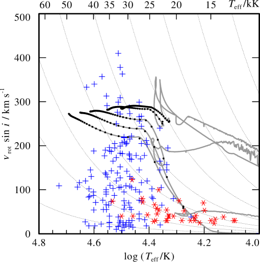
Figure 1.: Rotational velocities as a function of $T_{\rm eff}$ for OB stars from the VLT-Flames survey of massive stars with evolutionary masses above 15 $M_{\odot}$. Luminosity classes are shown as blue pluses (luminosity classes ii-v) and red stars (luminosity class i). The LMC evolutionary tracks from Brott et al. (2011), which include the bi-stability-jump, are shown in grey with initial $\varv_{\rm rot}=250$ km/s for five masses of 15, 20, 30, 40 and 60 $M_{\odot}$. It can be seen that the critical mass for bi-stability braking in the LMC is $\sim$35$M_{\odot}$. The steepness of these tracks may be compared to the case of angular momentum conservation (drawn as grey dotted background lines). The black dots on the tracks represent time-steps of $10^{5}$ years. See Vink et al. (2010) for more details.

2 Spherical winds: from CAK to a new formulation

For optically thin O-star winds two distinct approaches are in use to compute the relevant (line) opacity $\kappa$ and the resulting radiative acceleration $g_{\rm rad}$. In the first method, the line acceleration is expressed as a function of the velocity gradient $(dv/dr)$ in the CAK theory of Castor et al. (1975). In the second approach, the line acceleration is expressed as a function of radius $r$ (Lucy & Solomon 1970), which has been implemented in Monte Carlo models, see Fig. 2 (Müller & Vink 2008).

Figure 2.: The dots represent the dimensionless radiative line acceleration ${g_{\rm rad}^{\rm line}}\,({r})$ versus radial distance $r$ for a typical O5V-star, as derived from Monte Carlo simulations. In order to determine the line acceleration parameters, the simulated values were fitted with a non-linear model equation (see Müller & Vink 2008) resulting in the solid curve (wind parameters then follow from an iteration process).

2.1 Instabilities and wind clumping

Because of the non-linear character of the equation of motion, the CAK solution is complex, with the physics involving instabilities due to the line-deshadowing instability LDI (see Owocki 2015). One of the key implications of the LDI is that the time-averaged $\dot{M}$ is not expected to be affected by wind clumping, as it has the same (average) $\dot{M}$ as the CAK solution. However, the shocked velocity structure and associated density are expected to result in changes of the mass-loss diagnostics.

$\dot{M}$ diagnostics that is dependent on the square of the density, such as H$\alpha$, will result in a square-root reduction of $\dot{M}$ (Hillier 1991; Hamann et al. 2008), whilst ultraviolet P Cygni lines such as Pv depend linearly on density (Puls et al. 2008). Most analyses have been based on the assumption of optically thin clumps, but clumped winds are porous, with a range of clump sizes and optical depths. Oskinova et al. (2007) employed an effective opacity concept for line-profile modelling of the O supergiant $\zeta$ Pup, showing that the most pronounced effect involves resonance lines like Pv, which can be reproduced by their macro-clumping approach (see also Sundqvist et al. 2010).

In the traditional view of line-driven winds of O-type stars via the CAK theory and the associated LDI, clumping would be expected to develop in the wind when the wind velocities are large enough to produce shocked structures. For O star winds, this is thought to occur at about half the terminal wind velocity at about 1.5 stellar radii. Observational indications from linear polarization (e.g. Davies et al. 2005; 2007) however show that clumping already exists close to the stellar photosphere. Cantiello et al. (2009) suggested that convection in the sub-surface layers associated with the iron opacity peak could be the root cause of wind clumping.

2.2 High Eddington $\Gamma$ factor

We have discussed the optically thin stellar winds of normal O stars, but at certain luminosities the winds may become optically thick. What this means is that the wind optical depth $\tau$ crosses unity and thereby also the wind efficiency number $\eta$ crosses unity (Vink & Gräfener 2012, using data and model results by Martins et al. 2008).

For (super)O-stars (on steroids) this means the absorption line dominated spectrum turns into a Wolf-Rayet type spectrum of the hydrogen-rich (and nitrogen (N) rich) variety: WNh. Bestenlehner et al. (2014) studied this transition between optically thin (O star) and optically thick (Of/WN; WNh) stars in the context of the VLT-Flames Tarantula survey (VFTS; Evans et al. 2011) by analyzing 62 objects with cmfgen (Hillier & Miller 1998), confirming the predicted kink of Vink et al. (2011), see Fig. 3.

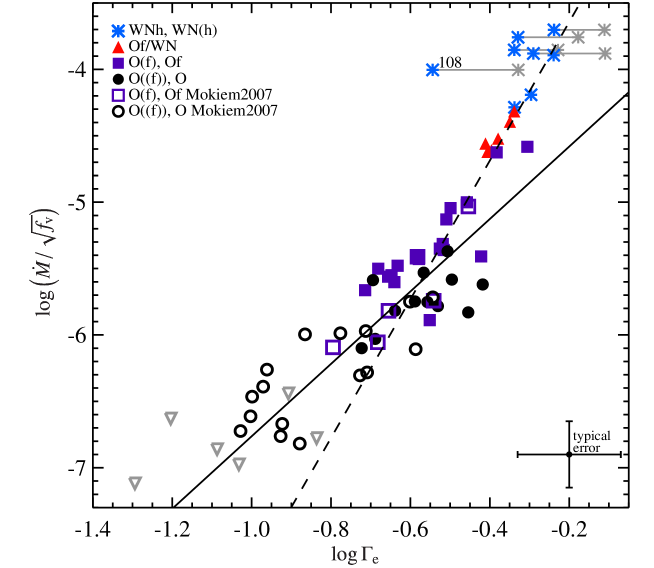
Figure 3.: Unclumped $\log\dot{M}$ vs. $\log\Gamma_{\rm e}$. Solid line: $\dot{M}-\Gamma$ relation for O stars. The different symbols indicate stellar sub-classes. Dashed line: the steeper slope of the Of/WN and WNh stars – forming a kink. The grey asterisks indicate the position of the stars with $Y>0.75$ under the assumption of core He-burning. The grey upside down triangles are stars from Mokiem et al. (2007) which only have an upper limit in $\dot{M}$ are excluded from the fit. See Bestenlehner et al. (2014).

This means that mass-loss rates in stellar evolution should not be considered as a function of luminosity, but the $L/M$ ratio related to the Eddington $\Gamma$ factor instead (Vink 2015). Another relevant factor (besides metallicity) is that of the effective temperature (see below).

2.3 The Bi-stability jump

At certain specific effective temperatures, 21 000 K, and again at 10 000 K the ionization of iron (Fe) changes dramatically from Fe iv to Fe iii, and at cooler temperatures from Fe iii to Fe ii, causing a dramatic increase in the line acceleration below the sonic point and in the predicted mass-loss rate as a result (Vink et al. 1999; Petrov et al. 2016). These transitions are referred to as bi-stability jumps (Pauldrach & Puls 1990; Lamers et al. (1995). These jumps may play an important role in stellar wind braking as discussed above, but the mechanism may also play a role in the 2D latitudinal dependence of winds between a hotter pole and a cooler equator, as in the rotationally-induced bi-stability mechanism of Lamers & Pauldrach (1991) for B[e] stars that is shown in Fig. 4 and discussed in more detail below.

3 2D stellar winds and disks

Until 3D radiation transfer models with 3D hydrodynamics become available, theorists have been forced to make assumptions with respect to either the radiative transfer (e.g. by assuming a power law approximation for the line force due to CAK or the hydrodynamics, e.g. by assuming an empirically motivated wind terminal velocity in Monte Carlo predictions (Abbott & Lucy 1985). Although recent 1D and 2D models of Müller & Vink (2008; 2014) no longer require the assumption of an empirical terminal wind velocity.

There are 2D wind models on the market that predict the wind mass loss predominately emanating from the equator, whilst other models predict higher mass-loss rates from the pole. The first effect of stellar rotation that needs to be taken into account is that of a reduced effective gravity at the stellar equator (Friend & Abbott 1986), with 2D modifications and expansions by e.g. Bjorkman & Cassinelli (1993) and Cure (2004). These 2D equatorial wind models might potentially result in the required equatorial disk formation for Be and B[e] stars. However, due to a combination of non-radial line forces and the result of the Von Zeipel (1924) effect – resulting in a hotter pole – equatorial disk formation is suppressed, and a stronger polar wind is expected instead (Owocki et al. 1996, Petrenz & Puls 2000). Furthermore, disks might be ablated due to the strong radiation fields around OB stars (Kee et al. 2016).

Is there no hope to form an equatorial outflow using radiative pressure? The best physical model that is available is that of the rotationally-induced bi-stability model of Lamers & Pauldrach (1991), improved with appropriate Fe line driving models in Pelupessy et al. (2000). The key point of this model is that there is a natural temperature transition as a function of stellar latitude as can be noted in Fig. 4. The hot pole drives a fast (several 1000s km/s) hot-star wind driven by high ionization stages (since Vink et al. (1999) we know this should be Fe iv and not C iv), whilst the cooler equator drives a slow wind (100s of km/s) driven by lower ionization stages of Fe.

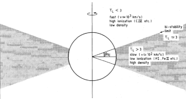
Figure 4.: Note the temperature transition as a function of stellar latitude due to Von Zeipel (1924). The hot pole drives a fast (several 1000s km/s) hot-star wind driven by high ionization stages of Fe iv, whilst the cooler equator drives a slower wind (100s of km/s) driven by lower ionization stages of Fe. Figure from Lamers & Pauldrach 1991.

The author is well aware that for Be stars, and now also B[e] stars (see later), the disks seem to be in Keplerian motion, with outflow velocities being less evident. Such rotating disks may well be described by a viscous disk (see Lee et al. 1991; Okazaki 2001; Carciofi et al. 2012) but such a viscous disk would still not explain why disk formation occurs in the first place. The prevalence of disks at spectral types B (in close proximity to the temperature of the bi-stability jump) means that the rotationally-induced mechanism remains an attractive one.

In any case, the key point from the different theoretical options is that mass loss from the equator results in more angular momentum loss than would 1D spherical or 2D polar mass loss, so we need 2D data to test theoretical models.

4 The tool of spectropolarimetry

The principle of linear spectropolarimetry is quite simple. The tool is based on the assumption that free electrons in an extended circumstellar medium scatter continuum radiation from the central star, revealing a certain level of linear polarization. If the projected electron distribution is perfectly circular, e.g. when the gas is spherically symmetric or when a disk is observed face-on, the linear Stokes vectors $Q$ and $U$ cancel, and no polarization is detected (as long as the object is spatially unresolved). If the geometry is not circular but involves an inclined disk, this would result in net continuum polarization.

Figure 5.: Cartoons representing line depolarization (left hand side) and compact line emission scattered off a rotating disk (right hand side) as triplots and $QU$ diagrams. Stokes $I$ profiles are shown in the lower triplot panels, % Pol in the middle panels, and the position angles (PAs) are given in the upper triplot panels. Line depolarization is as broad as the Stokes I emission, while the line polarization is narrow by comparison. Depolarization translates into $QU$ space as a linear excursion (left hand side), whilst a line polarization PA flip is associated with a $QU$ loop (right hand side).

One of the advantages of spectropolarimetry over continuum polarimetry is that one can perform differential polarimetry between a spectral line and the continuum independent of instrumental/interstellar polarization (ISP). The H$\alpha$ depolarization “line effect” utilizes the expectation that hydrogen recombination lines arise over a much larger volume than the continuum and becomes depolarized (see the left hand side of Fig. 5). Depolarization immediately indicates the presence (or absence) of aspherical geometries, such as disks, on spatial scales that cannot be imaged with the world’s largest telescopes.

The basic idea of the technique was explored in the 1970s by e.g. Poeckert & Marlborough (1976) who employed narrow-band filters to show that Be stars have disks as around 55% of their objects showed the depolarization line effect. It took another couple of decades before interferometry confirmed these findings. Interestingly, in a recent study of peculiar O stars, Vink et al. (2009) did not find evidence for the presence of disks in Oe stars – the alleged counterparts of classical Be stars – although the first detection of a line effect in an Oe star (HD 45314) was also reported.

In general we divide the polarimetric data into bins corresponding to 0.1% polarization, the typical error bar (although the numbers from photon statistics are at least a factor 10 better). We also present the data in $QU$ diagrams. For the case of line depolarization this translates into a linear excursion from the clusters of points that represents the continuum ($P^{2}=Q^{2}+U^{2}$) with the excursion showing the trend when the polarization moves in and out of line center.

A most relevant quantity involves the detection limit, which is inversely dependent on the signal-to-noise ratio (SNR) and the contrast of the emission line to the continuum. The detection limit $\Delta P_{\rm limit}$ can be represented by:

$$\Delta P_{\rm limit}(\%)=\frac{100}{SNR}\times\frac{l/c}{l/c-1}$$

where $l/c$ refers to the line-to-continuum contrast. This detection limit is most useful for objects with strong emission lines, such as H$\alpha$ emission in Luminous Blue Variables (LBVs; Humphreys & Davidson 1994; Smith et al. 2004; Vink 2012), where the emission completely overwhelms underlying photospheric absorption. In general, one wishes to achieve a signal-to-noise ratio (in the continuum) of about 1000, corresponding to changes in the amount of linear polarization of 0.1%. We should be able to infer asymmetry degrees in the form of equator/pole density ratios, $\rho_{\rm eq}/\rho_{\rm pole}$ of $\sim$1.25, or larger (Harries 2000), with some small additional dependence on the shape and inclination of the disk.

Most of the linear line polarimetry work of the last two decades has indeed concerned line depolarization, but in the following we will see that in some cases there is evidence for intrinsic line polarization, predicted by Wood et al. (1993) and found observationally in pre-main sequence (PMS) T Tauri and Herbig Ae/Be stars by our group (Vink et al. 2002, 2003, 2005b, Mottram et al. 2007). In such cases line photons are thought to originate from a compact source, e.g. as a result of (magnetospheric) accretion. These compact photons are scattered off a rotating disk, leading to a flip in the position angle (PA), and resulting in a rounded loop (rather than a linear excursion) in the $QU$ diagram (sketched on the right hand side of Fig. 5).

5 Depolarization results for B[e] supergiants and LBVs

Line depolarization has been observed in a plethora of massive stars, involving B[e] supergiants (e.g. Oudmaijer & Drew 1999), post Red Supergiants (Patel et al. 2008), as well as LBVs (see below). In all these cases the incidence rate of “line effects” appears to be consistent with the Be star results, i.e. 50-60%. Furthermore, the measured PA of the line-effect stars shows great consistency with PA constraints from other techniques, providing further evidence that the tool is capable of discovering and constraining circumstellar disks.

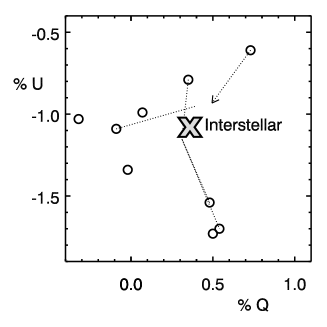
Figure 6.: H$\alpha$ polarimetry of the Luminous Blue Variable AG Car. The triplot on the left hand side reveals line depolarization. The large cross on the right hand side denotes the measured polarization at line center (constant with time), whilst the open circles represent the continuum measurements that vary with time, indicating wind clumping. See Davies et al. (2005, 2007) for details.

Davies et al. (2005) performed a spectropolarimetry survey of LBVs in the Galaxy and Magellanic Clouds and found some intriguing surprises. At first sight the results suggested the presence of disks (or equatorial outflows), as the incidence rate of line effects was inferred to be $>$50%. This is notably higher than that of their evolutionary neighbors O and Wolf-Rayet stars, with incidence rates of $<$25% (Vink et al. 2009) and $\sim$15% (Harries et al. 1998) respectively. However, when Davies et al. plotted the results of AG Car in a $QU$ diagram (see Fig. 6) they noticed that the level of polarization varied with time, which was interpreted as the manifestation of wind clumping.

Subsequent modelling by Davies et al. (2007) shows how time-variable linear polarization might become a powerful tool to constrain clump sizes and numbers. These constraints have already been employed in theoretical studies regarding the origin of wind clumping in sub-surface convection layers (Cantiello et al. 2009) and the effects of wind clumping on predicted mass-loss rates (Muijres et al. 2011).

One may attempt to derive the number of convective cells by dividing the stellar surface area by the size of a convective cell. For main-sequence O-type stars, pressure scale heights are in a range 0.04-0.24 $R_{\odot}$, corresponding to a total number of clumps of $6\times 10^{3}-6\times 10^{4}$. These numbers may be tested through linear polarization variability observations:

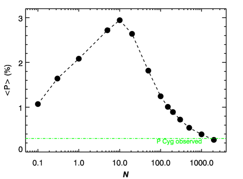
Figure 7.: Time-averaged polarization over a range of ejection rates (per wind flow-time). At $\mathcal{N}\sim 20$, the optical depth per clump exceeds unity and the overall polarization drops (see Davies et al. 2007 for details). The observed amount of polarization is indicated by the dash-dotted line. Note that there are two ejection-rate regimes where the observed level of polarization may be achieved for P Cygni.

Davies et al. (2005) showed that more than half the luminous blue variables (LBVs) are intrinsically polarized. As the polarization angle was found to change irregularly with time, the observed line effects were considered to be the result of wind clumping. An example of a model predicting the time-averaged polarization for the LBV P Cygni is shown in Fig. 7. There are two regimes where the observed polarization level may be reached. One is where the ejection rate is very low and only a few very optically thick clumps are ejected; the other scenario involves that of a very large number of clumps. The two scenarios may be distinguished via time-resolved polarimetry. Given the short timescale of the polarization variability data, we assume that LBV winds consist of thousands of clumps near the photosphere. However, for main-sequence O stars the derivation of wind-clump sizes from polarimetry has not yet been feasible as very high signal-to-noise data are required. LBVs offer an excellent opportunity for constraining the number of clumps from polarization variations because of the combination of higher mass-loss rates and lower terminal velocities. Davies et al. (2007) found that in order to produce the polarization variability of P Cygni, the wind should consist of some 1000 clumps per wind flow-time. In order to check whether this is compatible with subsurface convection being the root cause for clumping, we would need to consider the sub-surface convective regions of an object with properties similar to those of P Cygni. Because of the lower gravity of P Cyg the pressure scale height is about 4 $R_{\odot}$, i.e. significantly larger than for O-type stars. Therefore, the same estimate for the number of clumps as done for the O stars yields some 500 clumps per wind-flow time, which is consistent with that derived from the polarization data.

5.1 Monte Carlo disk models

Figure 8.: Monte Carlo line polarimetry for the case of a disk with an inner hole (left hand side) and without an inner hole – a result of the finite size of the star (right hand side). From Vink, Harries & Drew (2005a).

We now return to disks. Motivated by the almost ubiquitous incidence of $QU$ loops in T Tauri and Herbig Ae stars (Vink et al. 2002, 2003, 2005b), Vink et al. (2005a) decided to develop numerical polarization models of line emission scattered off Keplerian rotating disks using a 3D Monte Carlo code, with and without a disk inner hole. Figure 8 shows a marked difference between scattering off a disk that reaches the stellar photosphere (right hand side), and a disk with a significant inner hole (left hand side). The single PA flip on the left-hand side is similar to that predicted analytically (Wood et al. 1993), but the double PA flip on the right-hand side – associated with the undisrupted disk – came as a surprise at the time. The effect is the result of the geometrically correct treatment of the finite-sized stars that interacts with the disk’s rotational velocity field. Our numerical models demonstrated the potential of line polarimetry (as opposed to depolarization, where no velocity information can be gleaned) in establishing not only the disk inclination, but also the size of disk inner holes.

As far as we are aware linear line polarimetry is as yet the only method capable of determining disk holes sizes on the required spatial scales, to test both magnetospheric accretion in the young star context, and wind driving for massive stars, as either of these processes are crucially determined within the first few stellar radii from the stellar surface.

5.2 Evidence for disk rotation in B[e] stars

Figure 9.: The polarization spectrum of the B[e] star HD 87643, and the corrected spectrum of the star. The PA rotation suggests rotation of the disk. For more details, see Oudmaijer et al. (1998) and Oudmaijer & Drew (1999).

Returning to evolved objects such as B[e] stars we may perform similar observations as we performed on PMS stars. The best example of line spectropolarimetry in B[e] stars is given in Fig. 9. It shows the unambiguous presence of rotation as noted in the change of the position angle. Spectroscopic and spectropolarimetric data for this object have been presented and analyzed in detail by Oudmaijer et al. (1998) and Oudmaijer & Drew (1999). A comparison with the schematic model calculations by Wood et al. (1993) and Vink et al. (2005a) indicates that the polarization profile may indeed be reproduced with a rotating circumstellar disk.

6 Outlook

The first question to address is whether progress is expected to mostly come from theory, modelling or observations. Monte Carlo models (e.g. for disks with and without inner holes as shown in Fig. 8) are rather versatile, so modelling is not an issue. However, in order to be able to test the subtle differences shown in in Fig. 8, we require data with higher S/N.

We are at an exciting time in history, as we are on the verge of making a huge breakthrough. Normal stellar Stokes I spectroscopy at sufficient S/N has been performed for over 100 years, but because linear spectropolarimetry is photon hungry (as for most relevant cases the degree of polarization is just of order of $\sim$1%), we are about to enter a completely new era: that of of extremely large telescopes, providing us sufficient S/N to utilize the tool to its full potential.

A second new aspect will be time dependence. For B[e] stars linear polarization measurements have generally been attributed to the presence of disks (Magalhaes 1992; Oudmaijer & Drew 1999), but before we can unquestionably proof this, we would need to check that the PA is constant with time. The situation of the LBVs, where we now know the PA is variable (Davies et al. 2005), should be considered as a warning sign.

Finally, spectropolarimetric monitoring will be needed in order to probe 3D structures, such as wind clumping and/or rotating disk structures. This may become possible with future space instruments such as Arago/UVMag (Neiner 2015).

References

- (1) Abbott, D. C., & Lucy, L. B. 1985, ApJ 288, 679
- (2) Bestenlehner, J. M., Gräfener, G., Vink, J. S., et al. 2014, A&A 570, A38
- Bjorkman & Cassinelli (1993) Bjorkman, J. E., & Cassinelli, J. P. 1993, ApJ 409, 429
- Brott et al. (2011) Brott, I., de Mink, S. E., Cantiello, M., et al. 2011, A&A 530, A115
- (5) Cantiello, M., Langer, N., Brott, I., et al. 2009, A&A 499, 279
- Carciofi et al. (2012) Carciofi, A. C., Bjorkman, J. E., Otero, S. A., et al. 2012, ApJL 744, L15
- (7) Castor, J. I., Abbott, D. C., & Klein, R. I. 1975, ApJ 195, 157
- Curé (2004) Curé, M. 2004, ApJ 614, 929
- Davies et al. (2005) Davies, B., Oudmaijer, R. D., & Vink, J. S. 2005, A&A 439, 1107
- Davies et al. (2007) Davies, B., Vink, J. S., & Oudmaijer, R. D. 2007, A&A 469, 1045
- (11) Evans, C. J., Taylor, W. D., Hénault-Brunet, V., et al. 2011, A&A 530, A108
- Friend & Abbott (1986) Friend, D. B., & Abbott, D. C. 1986, ApJ 311, 701
- Groh et al. (2006) Groh, J. H., Hillier, D. J., & Damineli, A. 2006, ApJL 638, L33
- (14) Hamann, W.-R., Feldmeier, A., & Oskinova, L. M. 2008, Clumping in Hot-Star Winds
- Harries (2000) Harries, T. J. 2000, MNRAS 315, 722
- (16) Hillier, D. J. 1991, A&A 247, 455
- (17) Hillier, D. J., & Miller, D. L. 1998, ApJ 496, 407
- (18) Humphreys, R. M., & Davidson, K. 1994, PASP 106, 1025
- Justham et al. (2014) Justham, S., Podsiadlowski, P., & Vink, J. S. 2014, ApJ 796, 121
- Kee et al. (2016) Kee, N. D., Owocki, S., & Sundqvist, J. O. 2016, MNRAS 458, 2323
- Lamers & Pauldrach (1991) Lamers, H. J. G., & Pauldrach, A. W. A. 1991, A&A 244, L5
- (22) Lamers, H. J. G. L. M., Snow, T. P., & Lindholm, D. M. 1995, ApJ 455, 269
- Lee et al. (1991) Lee, U., Osaki, Y., & Saio, H. 1991, MNRAS, 250, 432
- (24) Lucy, L. B., & Solomon, P. M. 1970, ApJ 159, 879
- Magalhaes (1992) Magalhaes, A. M. 1992, ApJ 398, 286
- (26) Martins, F., Hillier, D. J., Paumard, T., et al. 2008, A&A 478, 219
- Mokiem et al. (2007) Mokiem, M. R., de Koter, A., Evans, C. J., et al. 2007, A&A 465, 1003
- Mottram et al. (2007) Mottram, J. C., Vink, J. S., Oudmaijer, R. D., & Patel, M. 2007, MNRAS 377, 1363
- Muijres et al. (2011) Muijres, L. E., de Koter, A., Vink, J. S., et al. 2011, A&A 526, 32
- (30) Müller, P. E., & Vink, J. S. 2008, A&A 492, 493
- Müller & Vink (2014) Müller, P. E., & Vink, J. S. 2014, A&A 564, A57
- Neiner (2015) Neiner, C. 2015, New Windows on Massive Stars, 307, 389
- Okazaki (2001) Okazaki, A. T. 2001, PASJ 53, 119
- (34) Oskinova, L. M., Hamann, W.-R., & Feldmeier, A. 2007, A&A 476, 1331
- Oudmaijer & Drew (1999) Oudmaijer, R. D., & Drew, J. E. 1999, MNRAS 305, 166
- Oudmaijer et al. (1998) Oudmaijer, R. D., Proga, D., Drew, J. E., & de Winter, D. 1998, MNRAS 300, 170
- (37) Owocki, S. P. 2015, Very Massive Stars in the Local Universe, 412, 113
- Owocki et al. (1996) Owocki, S. P., Cranmer, S. R., & Gayley, K. G. 1996, ApJL 472, L115
- Patel et al. (2008) Patel, M., Oudmaijer, R. D., Vink, J. S., et al. 2008, MNRAS 385, 967
- (40) Pauldrach, A. W. A., & Puls, J. 1990, A&A 237, 409
- Petrenz & Puls (2000) Petrenz, P., & Puls, J. 2000, A&A 358, 956
- (42) Petrov, B., Vink, J. S., & Gräfener, G. 2016, MNRAS 458, 1999
- Podsiadlowski et al. (2006) Podsiadlowski, P., Morris, T. S., & Ivanova, N. 2006, Stars with the B[e] Phenomenon, 355, 259
- Poeckert & Marlborough (1976) Poeckert, R., & Marlborough, J. M. 1976, ApJ 206, 182
- (45) Puls, J., Vink, J. S., & Najarro, F. 2008, ARAA 16, 209
- (46) Smith, N., Vink, J. S., & de Koter, A. 2004, ApJ 615, 475
- (47) Sundqvist, J. O., Puls, J., & Feldmeier, A. 2010, A&A 510, A11
- (48) Vink, J. S. 2012, Eta Carinae and the Supernova Impostors, 384, 221
- (49) Vink, J. S. 2015, Very Massive Stars in the Local Universe, 412, 77
- (50) Vink, J. S., & Gräfener, G. 2012, ApJL 751, L34
- (51) Vink, J. S., de Koter, A., & Lamers, H. J. G. L. M. 1999, A&A 350, 181
- (52) Vink, J. S., de Koter, A., & Lamers, H. J. G. L. M. 2000, A&A 362, 295
- Vink et al. (2002) Vink, J. S., Drew, J. E., Harries, T. J., & Oudmaijer, R. D. 2002, MNRAS 337, 356
- Vink et al. (2003) Vink, J. S., Drew, J. E., Harries, T. J., Oudmaijer, R. D., & Unruh, Y. C. 2003, A&A 406, 703
- Vink et al. (2005) Vink, J. S., Harries, T. J., & Drew, J. E. 2005a, A&A 430, 213
- Vink et al. (2005) Vink, J. S., Drew, J. E., Harries, T. J., Oudmaijer, R. D., & Unruh, Y. 2005b, MNRAS 359, 1049
- Vink et al. (2009) Vink, J. S., Davies, B., Harries, T. J., Oudmaijer, R. D., & Walborn, N. R. 2009, A&A 505, 743
- Vink et al. (2010) Vink, J. S., Brott, I., Gräfener, G., et al. 2010, A&A 512, L7
- (59) Vink, J. S., Muijres, L. E., Anthonisse, B., et al. 2011, A&A 531, A132
- von Zeipel (1924) von Zeipel, H. 1924, MNRAS 84, 665
- Wood et al. (1993) Wood, K., Brown, J. C., & Fox, G. K. 1993, A&A 271, 492