Recombining Tree Approximations for Optimal Stopping for Diffusions

Abstract

In this paper we develop two numerical methods for optimal stopping in the framework of one dimensional diffusion. Both of the methods use the Skorohod embedding in order to construct recombining tree approximations for diffusions with general coefficients. This technique allows us to determine convergence rates and construct nearly optimal stopping times which are optimal at the same rate. Finally, we demonstrate the efficiency of our schemes on several models.

1 Introduction

It is well known that pricing American options leads to optimal stopping problems (see [17, 18]). For finite maturity optimal stopping problems, there are no explicit solutions even in the relatively simple framework where the diffusion process is a standard Brownian motion. Motivated by the calculations of American options prices in local volatility models we develop numerical schemes for optimal stopping in the framework of one dimensional diffusion. In particular, we develop tree based approximations. In general for non-constant volatility models the nodes of the tree approximation trees do not recombine and this fact results in an exponential and thus a computationally explosive tree that cannot be used especially in pricing American options. We will present two novel ways of constructing recombining trees.

The first numerical scheme we propose, a recombining binomial tree (on a uniform time and space lattice), is based on correlated random walks. A correlated random walk is a generalized random walk in the sense that the increments are not identically and independently distributed and the one we introduce has one step memory. The idea to use correlated random walks for approximating diffusion processes goes back to [16], where the authors studied the weak convergence of correlated random walks to Markov diffusions. The disadvantage of the weak convergence approach is that it can not provide error estimates. Moreover, the weak convergence result can not be applied for numerical computations of the optimal stopping time. In order to obtain error estimates for the approximations and calculate numerically the optimal control we should consider all the processes on the same probability space, and so methods based on strong approximation theorems come into picture. In this paper we apply the Skorokhod embedding technique for ”small” perturbations of the correlated random walks. Our approach can be seen as an extension of recombining tree approximations from the case when a stock evolves according to the geometrical Brownian motion to the case of a more general diffusion evolution. This particular case required the Skorokhod embedding into the Brownian motion (with a constant variance) and it was treated in the more general game options case in [21, 12].

Under boundness and Lipschitz conditions on the drift and volatility of the diffusion, we obtain error estimates of order $O(n^{-1/4})$. Moreover we show how to construct a stopping time which is optimal up to the same order. In fact, we consider a more general setup where the diffusion process might have absorbing barriers. Clearly, most of the local volatility modes which are used in practice (for instance, the CEV model [9] and the CIR model [10]) do not satisfy the above conditions. Still, by choosing an appropriate absorbing barriers for these models, we can efficiently approximate the original models, and for the absorbed diffusions, which satisfy the above conditions, we apply our results.

Our second numerical scheme is a recombining trinomial tree, which is obtained by directly sampling the original process at suitable chosen random intervals. In this method we relax the continuity assumption and work with diffusions with measurable coefficients, e.g. the coefficients can be discontinuous, while we keep the boundedness conditions. (See Section 5.5 for an example). The main idea is to construct a sequence of random times such that the increment of the diffusion between two sequel times belongs to some fixed set of the form $\left\{-\bar{\sigma}\sqrt{\frac{T}{n}},0,\bar{\sigma}\sqrt{\frac{T}{n}}\right\}$ and the expectation of the difference between two sequel times equals to $\frac{T}{n}$. Here $n$ is the discretization parameter and $T$ is the maturity date. This idea is inspired by the recent work [2, 1] where the authors applied Skorohod embedding in order to obtain an Euler approximation of irregular one dimensional diffusions. Following their methodology we construct an exact scheme along stopping times. The constructions are different and in particular, in contrast to the above papers we introduce a recombining tree approximation. The above papers do provide error estimate (in fact they are of the same order as our error estimates) for the expected value of a function of the terminal value (from mathematical finance point of view, this can be viewed as European Vanilla options). Since we deal with American options, our proof requires additional machinery which allows to treat stopping times.

The second method is more direct and does not require the construction of a diffusion perturbation. In particular it can be used for the computations of Barrier options prices; see Remark 4.1. As we do for the first method, we obtain error estimates of order $O(n^{-1/4})$ and construct a stopping time which is optimal up to the same order.

Comparison with other numerical schemes. The most well-known approach to evaluate American options in one dimension is the finite difference scheme called the projected SOR method, see e.g. [28]. As opposed to a tree based scheme, the finite difference scheme needs to artificially restrict the domain and impose boundary conditions to fill in the entire lattice. The usual approach is the so-called far-field boundary condition (as is done in [28]). See the discussion in [29]. The main problem is that it is not known how far is sufficient and the error is hard to quantify. This problem was addressed recently by [29] for put options written on CEV models by what they call an artificial boundary method, which is model dependent in that an exact boundary condition is derived that is then embedded into the numerical scheme. (In fact, the PDE is transformed into a new PDE which satisfies a Neumann boundary condition.) This technique requires having an explicit expression of a Sturm-Lioville equation associated with the Laplace transform of the pricing equation. As an improvement over [29] the papers [30, 23] propose a numerical method based on solving the integral equations that the optimal exercise boundary satisfies. None of these papers discuss the convergence rate or prove that their proposed optimal exercise times are nearly optimal. We have the advantage of having an optimal stopping problem at the discrete level and without much additional effort are able to show that these stopping times are actually approximately optimal when applied to the continuous time problem. We compare our numerical results to these papers in Table 5.6.

Another popular approach is the Euler scheme or other Monte-Carlo based schemes (see e.g. [13, 3]). The grid structure allows for an efficient numerical computations of stochastic control problems via dynamical programming since computation of conditional expectation simplifies considerably. Compare this to the least squares method in [25] (also see [13]). Besides the computational complexity, the bias in the least squares is hard to characterize since it also relies on the choice of bases functions. Recently a hybrid approach was developed in [7]. (The scope of this paper is more general and is in the spirit of [25]). Our discussion above in comparing our proposed method to Monte-Carlo applies here. Moreover, although [7] provides a convergence rate analysis using PDE methods (requiring regularity assumptions on the coefficients, which our scheme does not need), our paper in addition can prove that the proposed stopping times from our numerical approximations are nearly optimal.

To summarize, our contributions are

• We build two recombining tree approximations for local volatility models, which considerably simplifies the computation of conditional expectations.

• By using the Skorohod embedding technique, we give a proof of the rate of convergence of the schemes.

• This technique in particular allows us to show that the stopping times constructed from the numerical approximations are nearly optimal and the error is of the same magnitude as the convergence rate.

This rest of the paper is organized as follows. In the next section we introduce the setup and introduce the two methods we propose and present the main theoretical results of the paper, namely Theorems 2.1 and 2.2 (see the last statements in subsections 2.2 and 2.3). Sections 3 and 4 are devoted to the proof of these respective results. In Section 5 we provide a detailed numerical analysis for both of our methods by applying them to various local volatility models.

2 Preliminaries and Main Results

2.1 The Setup

Let $\{W_{t}\}_{t=0}^{\infty}$ be a standard one dimensional Brownian motion, and let $Y_{t}$, $t\geq 0$ be a one dimensional diffusion

(2.1) $$dY_{t}=\sigma(Y_{t})dW_{t}+\mu(Y_{t})dt,\ \ Y_{0}=x.$$

Let $\{\mathcal{F}_{t}\}_{t=0}^{T}$ be a filtration which satisfies the usual conditions such that $Y_{t}$, $t\geq 0$ is an adapted process and $W_{t}$, $t\geq 0$ is a Brownian motion with respect to this filtration. We assume that the SDE (2.1) has a weak solution that is unique in law.

Introduce an absorbing barriers $B<C$ where $B\in[-\infty,\infty)$ and $C\in(-\infty,\infty]$. We assume that $x\in(B,C)$ and look at the absorbed stochastic process

$$X_{t}=\mathbb{I}_{t<\inf\{s:Y_{s}\notin(B,C)\}}Y_{t}+\mathbb{I}_{t\geq\inf\{s:Y_{s}\notin(B,C)\}}Y_{\inf\{s:Y_{s}\notin(B,C)\}},\ \ t\geq 0.$$

Motivated by the valuation of American options prices we study an optimal stopping problem with maturity date $T$ and a reward $f(t,X_{t})$, $t\in[0,T]$ where $f:[0,T]\times\mathbb{R}\rightarrow\mathbb{R}_{+}$ satisfies

(2.2) $$|f(t_{1},x_{1})-f(t_{2},x_{2})|\leq L\left((1+|x_{1}|)|t_{2}-t_{1}|+|x_{2}-x_{1}|\right),\ \ t_{1},t_{2}\in[0,T],\ \ x_{1},x_{2}\in\mathbb{R}$$

for some constant $L$. Clearly, payoffs of the form $f(t,x)=e^{-rt}(x-K)^{+}$ (call options) and $f(t,x)=e^{-rt}(K-x)^{+}$ (put options) fit in our setup.

The optimal stopping value is given by

(2.3) $$V=\sup_{\tau\in\mathcal{T}_{[0,T]}}\mathbb{E}[f(\tau,X_{\tau})],$$

where $\mathcal{T}_{[0,T]}$ is the set of stopping times in the interval $[0,T]$, with respect to the filtration $\mathcal{F}_{t}$, $t\geq 0$.

2.2 Binomial Approximation Scheme Via Random Walks

In this Section we assume the following.

Assumption 2.1.

The functions $\mu,\sigma:(B,C)\rightarrow\mathbb{R}$ are bounded and Lipschitz continuous. Moreover, $\sigma:(B,C)\rightarrow\mathbb{R}$ is strictly positive and uniformly bounded away from zero.

Binomial Approximation of the State Process. Fix $n\in\mathbb{N}$ and let $h=h(n):=\frac{T}{n}$ be the time discretization. Since the meaning is clear we will use $h$ instead of $h(n)$. Let $\xi^{(n)}_{1},...,\xi^{(n)}_{n}\in\{-1,1\}$ be a sequence of random variables. In the sequel, we always use the initial data $\xi^{(n)}_{0}\equiv 1$. Consider the random walk

$$X^{(n)}_{k}=x+\sqrt{h}\sum_{i=1}^{k}\xi^{(n)}_{i}\ \ k=0,1,...,n$$

with finite absorbing barriers $B_{n}<C_{n}$ where

$$B_{n}=x+\sqrt{h}\min\{k\in\mathbb{Z}\cap[-n-1,\infty):x+\sqrt{h}k>B+h^{1/3}\}$$

$$C_{n}=x+\sqrt{h}\max\{k\in\mathbb{Z}\cap(-\infty,n+1]:x+\sqrt{h}k<C-h^{1/3}\}.$$

Clearly, the process $\{X^{(n)}_{k}\}_{k=0}^{n}$ lies on the grid $x+\sqrt{h}\{-n,1-n,...,0,1,...,n\}$ (in fact because of the barriers its lie on a smaller grid).

We aim to construct a probabilistic structure so the pair $\{X^{(n)}_{k},\xi^{(n)}_{k}\}_{k=0}^{n}$ forms a Markov chain weakly approximating (with the right time change) the absorbed diffusion $X$. We look for a predictable (with respect the filtration generated by $\xi^{(n)}_{1},...,\xi^{(n)}_{n})$ process $\alpha^{(n)}=\{\alpha^{(n)}_{k}\}_{k=0}^{n}$ which is uniformly bounded (in space and $n$) and a probability measure $\mathbb{P}_{n}$ on $\sigma\{\xi^{(n)}_{1},...,\xi^{(n)}_{n}\}$ such that the perturbation defined by

(2.4) $$\hat{X}^{(n)}_{k}:=X^{(n)}_{k}+\sqrt{h}\alpha^{(n)}_{k}\xi^{(n)}_{k},\ \ k=0,1,...,n$$

is matching the first two moments of the diffusion $X$. Namely, we require that for any $k=1,...,n$ (on the event $B_{n}<X^{(n)}_{k-1}<C_{n}$)

(2.5) $$\mathbb{E}_{n}\left(\hat{X}^{(n)}_{k}-\hat{X}^{(n)}_{k-1}|\xi^{(n)}_{1},...,\xi^{(n)}_{k-1}\right)=h\mu(X^{(n)}_{k-1})+o(h),$$

(2.6) $$\mathbb{E}_{n}\left((\hat{X}^{(n)}_{k}-\hat{X}^{(n)}_{k-1})^{2}|\xi^{(n)}_{1},...,\xi^{(n)}_{k-1}\right)=h\sigma^{2}(X^{(n)}_{k-1})+o(h),$$

where we use the standard notation $o(h)$ to denote a random variable that converge to zero (as $h\downarrow 0$) a.s. after dividing by $h$. We also use the convention $O(h)$ to denote a random variable that is uniformly bounded after dividing by $h$.

From (2.4) it follows that $X^{(n)}_{k}-\hat{X}^{(n)}_{k}=o(1)$. Hence the convergence of $X^{(n)}$ is equivalent to the convergence of $\hat{X}^{(n)}$. It remains to solve the equations (2.5)–(2.6). By applying (2.4)–(2.5) together with the fact that $\alpha^{(n)}$ is predictable and $(\xi^{(n)})^{2}\equiv 1$ we get

$$\mathbb{E}_{n}\left((\hat{X}^{(n)}_{k}-\hat{X}^{(n)}_{k-1})^{2}|\xi^{(n)}_{1},...,\xi^{(n)}_{k-1}\right)=h(1+2\alpha^{(n)}_{k})+h\left((\alpha^{(n)}_{k})^{2}-(\alpha^{(n)}_{k-1})^{2}\right)+o(h).$$

This together with (2.6) gives that

$$\alpha^{(n)}_{k}=\frac{\sigma^{2}(X^{(n)}_{k-1})-1}{2},\ \ k=0,...,n$$

is a solution, where we set $X^{(n)}_{-1}\equiv x-\sqrt{h}$. Next, (2.5) yields that

$$\mathbb{E}_{n}\left(\xi^{(n)}_{k}|\xi^{(n)}_{1},...,\xi^{(n)}_{k-1}\right)=\frac{\alpha^{(n)}_{k-1}\xi^{(n)}_{k-1}+\sqrt{h}\mu(X^{(n)}_{k-1})}{1+\alpha^{(n)}_{k}}.$$

Recall that $\xi^{(n)}_{k}\in\{-1,1\}$. We conclude that the probability measure $\mathbb{P}_{n}$ is given by (prior to absorbing time)

(2.7) $$\mathbb{P}_{n}\left(\xi^{(n)}_{k}=\pm 1|\xi^{(n)}_{1},...,\xi^{(n)}_{k-1}\right)=\frac{1}{2}\left(1\pm\frac{\alpha^{(n)}_{k-1}\xi^{(n)}_{k-1}+\sqrt{h}\mu(X^{(n)}_{k-1})}{1+\alpha^{(n)}_{k}}\right),\ \ k=1,...,n.$$

In view of Assumption 2.1 we assume that $n$ is sufficiently large so $\mathbb{P}_{n}$ is indeed a probability measure. Moreover, we notice that $\alpha^{(n)}_{k-1}=\frac{\sigma^{2}(X^{(n)}_{k-1}-\sqrt{h}\xi^{(n)}_{k-1})-1}{2}$. Thus the right hand side of (2.7) is determined by $X^{(n)}_{k-1},\xi^{(n)}_{k-1}$, and so $\{X^{(n)}_{k},\xi^{(n)}_{k}\}_{k=0}^{n}$ is indeed a Markov chain.

Optimal Stopping Problem on a Binomial Tree. For any $n$ denote by $\mathcal{T}_{n}$ the (finite) set of all stopping times with respect to filtration $\sigma\{\xi^{(n)}_{1},...,\xi^{(n)}_{k}\}$, $k=0,...,n$. Introduce the optimal stopping value

(2.8) $$V_{n}:=\max_{\eta\in\mathcal{T}_{n}}\mathbb{E}_{n}[f(\eta h,X^{(n)}_{\eta})].$$

By using standard dynamical programming for optimal stopping (see [27] Chapter I) we can calculate $V_{n}$ and the rational stopping times by the following backward recursion. For any $k=0,1,...,n$ denote by $G^{(n)}_{k}$ all the points on the grid $x+\sqrt{h}\{-k,1-k,...,0,1,...,k\}$ which lie in the interval $[B_{n},C_{n}]$.

Define the functions

$$\mathfrak{J}^{(n)}_{k}:G^{(n)}_{k}\times\{-1,1\}\rightarrow\mathbb{R},\ \ k=0,1,...,n$$

$$\mathfrak{J}^{(n)}_{n}(z,y)=f(T,z).$$

For $k=0,1,...,n-1$

$$\mathfrak{J}^{(n)}_{k}(z,y)=\max\bigg{\{}f(kh,z),\sum_{i=1}^{2}\frac{1}{2}\left(1+(-1)^{i}\frac{\alpha^{\prime}y+\sqrt{h}\mu(z)}{1+\alpha}\right)\mathfrak{J}^{(n)}((k+1)h,z+(-1)^{i}\sqrt{h})\bigg{\}},\,\mbox{if}\ z\in(B_{n},C_{n}),$$

where $\alpha^{\prime}=\frac{\sigma^{2}(z-y\sqrt{h})-1}{2}$, $\alpha=\frac{\sigma^{2}(z)-1}{2}$, and

$$\mathfrak{J}^{(n)}_{k}(z,y)=\max_{k\leq m\leq n}f(mh,z)\quad\mbox{if}\ z\in\{B_{n},C_{n}\}.$$

We get that

$$V_{n}=\mathfrak{J}^{(n)}_{0}(x,1)$$

and the stopping time

(2.9) $$\eta^{*}_{n}=n\wedge\min\left\{k:\mathfrak{J}^{(n)}_{k}(X^{(n)}_{k},\xi^{(n)}_{k})=f(kh,X^{(n)}_{k})\right\}$$

is a rational stopping time. Namely,

$$V_{n}=\mathbb{E}_{n}[f(\eta^{*}_{n}h,X^{(n)}_{\eta^{*}_{n}})].$$

Skorohod Embedding. Before we formulate our first result let us introduce the Skorokhod embedding which allows to consider the random variables $\{\xi^{(n)}_{k},X^{(n)}_{k}\}_{k=0}^{n}$ (without changing their joint distribution) and the diffusion $X$ on the same probability space.

Set,

$$M_{t}:=x+\int_{0}^{t}\sigma(Y_{s})dW_{s}=Y_{t}-\int_{0}^{t}\mu(Y_{s})ds,\ \ t\geq 0.$$

The main idea is to embed the process

$$\tilde{X}^{(n)}_{k}:=X^{(n)}_{k}+\sqrt{h}(\alpha^{(n)}_{k}\xi^{(n)}_{k}-\alpha^{(n)}_{0}\xi^{(n)}_{0})-h\sum_{i=0}^{k-1}\mu(X^{(n)}_{i}),\ \ k=0,1,...,n$$

into the martingale $\{M_{t}\}_{t=0}^{\infty}$. Observe that prior the absorbing time, the process ${\{\tilde{X}^{(n)}_{k}\}}_{k=0}^{n}$ is a martingale with respect to the measure $\mathbb{P}_{n}$, and $\tilde{X}^{(n)}_{0}=x$.

Set,

$$\alpha^{(n)}_{0}=\frac{\sigma^{2}(x-\sqrt{h})-1}{2},\ \ \theta^{(n)}_{0}=0,\ \ \xi^{(n)}_{0}=1,\ \ X^{(n)}_{0}=x.$$

For $k=0,1,...,n-1$ define by recursion the following random variables

$$\alpha^{(n)}_{k+1}=\frac{\sigma^{2}(X^{(n)}_{k})-1}{2},$$

If $X^{(n)}_{k}\in(B_{n},C_{n})$ then

(2.10) $$\theta^{(n)}_{k+1}=\inf\left\{t>\theta^{(n)}_{k}:|M_{t}-M_{\theta^{(n)}_{k}}+\sqrt{h}\alpha^{(n)}_{k}\xi^{(n)}_{k}+h\mu(X^{(n)}_{k})|=\sqrt{h}(1+\alpha^{(n)}_{k+1})\right\},$$

(2.11) $$\xi^{(n)}_{k+1}=\mathbb{I}_{\theta^{(n)}_{k+1}<\infty}sgn\left(M_{\theta^{(n)}_{k+1}}-M_{\theta^{(n)}_{k}}+\sqrt{h}\alpha^{(n)}_{k}\xi^{(n)}_{k}+h\mu(X^{(n)}_{k})\right),$$

where we put $sgn(z)=1$ for $z>0$ and $=-1$ otherwise, and

(2.12) $$X^{(n)}_{k+1}=X^{(n)}_{k}+\sqrt{h}\xi^{(n)}_{k+1}.$$

If $X^{(n)}_{k}\notin(B_{n},C_{n})$ then $\theta^{(n)}_{k+1}=\theta^{(n)}_{k}+h$ and $X^{(n)}_{k+1}=X^{(n)}_{k}$. Set, $\Theta_{n}:=n\wedge\min\{k:X^{(n)}_{k}\notin(B_{n},C_{n})\}$ and observe that on the event $k<\Theta_{n}$, $\theta^{(n)}_{k+1}$ is the stopping time which corresponds to the Skorokhod embedding of the binary random variable with values in the (random) set $\{\pm\sqrt{h}(1+\alpha^{(n)}_{k+1})-\sqrt{h}\alpha^{(n)}_{k}\xi^{(n)}_{k}-h\mu(X^{(n)}_{k}\}$, into the martingale $\{M_{t}-M_{\theta^{(n)}_{k}}\}_{t\geq\theta^{(n)}_{k}}$. Moreover, the grid structure of $X^{(n)}$ implies that if $X^{(n)}_{k}\notin(B_{n},C_{n})$ then $X^{(n)}_{k}\in\{B_{n},C_{n}\}$.

Lemma 2.1.

The stopping times $\{\theta^{(n)}_{k}\}_{k=0}^{n}$ have a finite mean and the random variables $\{\xi^{(n)}_{k},X^{(n)}_{k}\}_{k=0}^{n}$ satisfy $(\ref{2.7})$.

Proof.

For sufficiently large $n$ we have that for any $k<n$

$$-\sqrt{h}(1+\alpha^{(n)}_{k+1})-\sqrt{h}\alpha^{(n)}_{k}\xi^{(n)}_{k}-h\mu(X^{(n)}_{k})<0<\sqrt{h}(1+\alpha^{(n)}_{k+1})-\sqrt{h}\alpha^{(n)}_{k}\xi^{(n)}_{k}-h\mu(X^{(n)}_{k}).$$

Thus by using the fact that volatility of the martingale $M$ is bounded away from zero, we conclude $\mathbb{E}(\theta^{(n)}_{k+1}-\theta^{(n)}_{k})<\infty$ for all $k<n$. Hence the stopping times $\{\theta^{(n)}_{k}\}_{k=0}^{n}$ have a finite mean.

Next, we establish (2.7) for the redefined $\{\xi^{(n)}_{k},X^{(n)}_{k}\}_{k=0}^{n}$. Fix $k$ and consider the event $k<\Theta_{n}$. From (2.10) we get

(2.13) $$M_{\theta^{(n)}_{k+1}}-M_{\theta^{(n)}_{k}}=\sqrt{h}(1+\alpha^{(n)}_{k+1})\xi^{(n)}_{k+1}-\sqrt{h}\alpha^{(n)}_{k}\xi^{(n)}_{k}-h\mu(X^{(n)}_{k}).$$

The stochastic process

$$\{M_{t}-M_{\theta^{(n)}_{k}}\}_{t=\theta^{(n)}_{k}}^{\theta^{(n)}_{k+1}}$$

is a bounded martingale and so $\mathbb{E}(M_{\theta^{(n)}_{k+1}}-M_{\theta^{(n)}_{k}}|\mathcal{F}_{\theta^{(n)}_{k}})=0$. Hence, from (2.13)

$$\mathbb{E}(\xi^{(n)}_{k+1}|\mathcal{F}_{\theta^{(n)}_{k}})=\frac{\alpha^{(n)}_{k}\xi^{(n)}_{k}+\sqrt{h}\mu(X^{(n)}_{k})}{1+\alpha^{(n)}_{k+1}}.$$

Since $\xi^{(n)}_{k+1}\in\{-1,1\}$ we arrive at

$$\mathbb{P}(\xi^{(n)}_{k+1}=\pm 1|\mathcal{F}_{\theta^{(n)}_{k}})=\frac{1}{2}\left(1\pm\frac{\alpha^{(n)}_{k}\xi^{(n)}_{k}+\sqrt{h}\mu(X^{(n)}_{k})}{1+\alpha^{(n)}_{k+1}}\right)$$

and conclude that (the above right hand side is $\sigma\{\xi^{(n)}_{1},...,\xi^{(n)}_{k}\}$ measurable) (2.7) holds true.

The first Main Result.

Theorem 2.1.

The values $V$ and $V_{n}$ defined by (2.3) and (2.8), respectively satisfy

$$|V_{n}-V|=O(n^{-1/4}).$$

Moreover, if we consider the random variables $\xi^{(n)}_{0},...,\xi^{(n)}_{n}$ defined by (2.10)–(2.12) and denote $\tau^{*}_{n}\in\mathcal{T}_{[0,T]}$ by $\tau^{*}_{n}=T\wedge\theta^{(n)}_{\eta^{*}_{n}}$, in which $\eta^{*}_{n}$ is from (2.9) and $\theta^{(n)}_{k}$ is from (2.10), then

$$V-\mathbb{E}[f(\tau^{*}_{n},X_{\tau^{*}_{n}})]=O(n^{-1/4}).$$

2.3 Trinomial Tree Approximation

In this section we relax the Lipschitz continuity requirement and assume the following.

Assumption 2.2.

The functions $\mu,\sigma,\frac{1}{\sigma}:(B,C)\rightarrow\mathbb{R}$ are bounded and measurable.

As our assumption indicates the results in this section apply for diffusions with discontinuous coefficients. See Section 5.5 for a pricing problem for a regime switching volatility example. See also [4] for other applications of such models.

Remark 2.1.

From the general theory of one dimensional, time–homogeneous SDE (see Section 5.5 in [19]) it follows that if $\sigma,\mu:\mathbb{R}$ are measurable functions such that $\sigma(z)\neq 0$ for all $z\in\mathbb{R}$ and the function $|\mu(z)|+|\sigma(z)|+|\sigma^{-1}(z)|$ is uniformly bonded, then the SDE (2.1) has a unique weak solution. Since the distribution of $X$ is determined only by the values of $\mu,\sigma$ in the interval $(B,C)$ we obtain (by letting $\sigma,\mu\equiv 1$ outside of the interval $(B,C)$) that Assumption 2.2 above is sufficient for an existence and uniqueness in law, of the absorbed diffusion $X$. Clearly, Assumption 2.1 is stronger than Assumption 2.2. A relevant reference here is [4] which not only considers the existence of weak solutions to SDEs but also of their Malliavin differentiability.

In this section we assume that $x,B,C\in\mathbb{Q}\cup\{-\infty,\infty\}$ (recall that the barriers $B$ and $C$ can take the values $-\infty$ and $\infty$, respectively), and so for sufficiently large $n$, we can choose a constant $\bar{\sigma}=\bar{\sigma}(n)>\sup_{y\in(B,C)}|\sigma(y)|+\sqrt{h}\sup_{y\in(B,C)}|\mu(y)|$ which satisfies $\frac{C-x}{\bar{\sigma}\sqrt{h}},\frac{x-B}{\bar{\sigma}\sqrt{h}}\in\mathbb{N}\cup\{\infty\}$.

Trinomial Approximation of the State Process. The main idea in this section is to find stopping times $0=\vartheta^{(n)}_{0}<\vartheta^{(n)}_{1}<...<\vartheta^{(n)}_{n}$, such that for any $k=0,1,...,n-1$

(2.14) $$X_{\vartheta^{(n)}_{k+1}}-X_{\vartheta^{(n)}_{k}}\in\{-\bar{\sigma}\sqrt{h},0,\bar{\sigma}\sqrt{h}\}\quad\mbox{and}\ \ \mathbb{E}(\vartheta^{(n)}_{k+1}-\vartheta^{(n)}_{k}|\mathcal{F}_{\vartheta^{(n)}_{k}})=h+O(h^{3/2}).$$

In this case the random variables $\{X_{\vartheta^{(n)}_{k}}\}_{k=0}^{n}$ lie on the grid $x+\bar{\sigma}\sqrt{h}\{-b_{n},1-b_{n},...,0,1,$
$...,c_{n}\}$ where $b_{n}=n\wedge\frac{x-B}{\bar{\sigma}\sqrt{h}}$ and $c_{n}=n\wedge\frac{C-x}{\bar{\sigma}\sqrt{h}}$. Moreover, we will see that

$$\max_{0\leq k\leq n}|\vartheta^{(n)}_{k}-kh|=O(\sqrt{h}).$$

Skorohod Embedding. Next, we describe the construction. For any initial position $B+\bar{\sigma}\sqrt{h}\leq X_{0}\leq C-\bar{\sigma}\sqrt{h}$ and $A\in[0,\bar{\sigma}\sqrt{h}]$ consider the stopping times

$$\rho^{X_{0}}_{A}=\inf\{t:|X_{t}-X_{0}|=A\}\ \ \mbox{and}$$

$$\kappa^{X_{0}}_{A}=\sum_{i=1}^{2}\mathbb{I}_{X_{\rho^{X_{0}}_{A}}=X_{0}+(-1)^{i}A}\inf\{t\geq\rho^{X_{0}}_{A}:X_{t}=X_{0}\ \mbox{or}\ X_{t}=X_{0}+(-1)^{i}\bar{\sigma}\sqrt{h}\}.$$

Observe that $X_{\kappa^{X_{0}}_{A}}-X_{0}\in\{-\bar{\sigma}\sqrt{h},0,\bar{\sigma}\sqrt{h}\}$. Let us prove the following lemma.

Lemma 2.2.

There exists a unique $\hat{A}=\hat{A}(X_{0},n)\in(0,\bar{\sigma}\sqrt{h}]$ such that $\mathbb{E}(\kappa^{X_{0}}_{\hat{A}})=h$.

Proof.

Clearly, for any $A_{1}<A_{2}$ $\kappa^{X_{0}}_{A_{1}}\leq\kappa^{X_{0}}_{A_{2}}$ a.s. Since $\kappa^{X_{0}}_{A_{1}}\neq\kappa^{X_{0}}_{A_{2}}$ for $A_{1}\neq A_{2}$ we conclude that the function $g(A):=\mathbb{E}(\kappa^{X_{0}}_{A})$ is strictly increasing which satisfies $g(0)=0$. Thus in order to complete the proof it remains to show that $g(\bar{\sigma}\sqrt{h})\geq h$. Observe that $g(\bar{\sigma}\sqrt{h})=\mathbb{E}(\rho^{X_{0}}_{\bar{\sigma}\sqrt{h}}).$ Assume (by contradiction) that $\mathbb{E}(\rho^{X_{0}}_{\bar{\sigma}\sqrt{h}})<h$. From the Itô isometry and the Jensen Inequality we obtain

$$\bar{\sigma}\sqrt{h}= \mathbb{E}|X_{\rho^{X_{0}}_{\bar{\sigma}\sqrt{h}}}-X_{0}|\leq\mathbb{E}\left|\int_{0}^{\rho^{X_{0}}_{\bar{\sigma}\sqrt{h}}}\sigma(X_{t})dW_{t}\right|+\mathbb{E}\left|\int_{0}^{\rho^{X_{0}}_{\bar{\sigma}\sqrt{h}}}\mu(X_{t})dt\right|$$

$$\leq \sup_{y\in\mathbb{R}}|\sigma(y)|\sqrt{\mathbb{E}(\rho^{X_{0}}_{\bar{\sigma}\sqrt{h}})}+\sup_{y\in\mathbb{R}}|\mu(y)|\mathbb{E}(\rho^{X_{0}}_{\bar{\sigma}\sqrt{h}})<\bar{\sigma}\sqrt{h}.$$

This clearly a contradiction, and the result follows.

Next, we recall the theory of exit times of Markov diffusions (see Section 5.5 in [19]). Set,

(2.15) $$p(y)=\int_{X_{0}}^{y}\exp\left(-2\int_{X_{0}}^{z}\frac{\mu(w)}{\sigma^{2}(w)}dw\right)dz,$$

$$G_{a,b}(y,z)=\frac{\left(p(y\wedge z)-p(a)\right)\left(p(b)-p(y\vee z)\right)}{p(b)-p(a)},\ \ a\leq y,z\leq b,$$

$$M_{a,b}(y)=\int_{a}^{b}\frac{2G_{a,b}(y,z)}{p^{\prime}(z)\sigma^{2}(z)}dz,\ \ y\in[a,b].$$

Then for any $A\in[0,\bar{\sigma}\sqrt{h}]$

(2.16) $$\mathbb{E}(\kappa^{X_{0}}_{A}) =\mathbb{E}(\rho^{X_{0}}_{A})+\mathbb{P}(X_{\rho^{X_{0}}_{A}}=X_{0}+A)M_{X_{0},X_{0}+\bar{\sigma}\sqrt{h}}(X_{0}+A)$$

$$+\mathbb{P}(X_{\rho^{X_{0}}_{A}}=X_{0}-A)M_{X_{0}-\bar{\sigma}\sqrt{h},X_{0}}(X_{0}-A)$$

$$=M_{X_{0}-A,X_{0}+A}(X_{0})+\frac{p(X_{0})-p(X_{0}-A)}{p(X_{0}+A)-p(X_{0}-A)}M_{X_{0},X_{0}+\bar{\sigma}\sqrt{h}}(X_{0}+A)$$

$$+\frac{p(X_{0}+A)-p(X_{0})}{p(X_{0}+A)-p(X_{0}-A)}M_{X_{0}-\bar{\sigma}\sqrt{h},X_{0}}(X_{0}-A)$$

and

$$q^{(1)}(X_{0},A):=\mathbb{P}(X_{\kappa^{X_{0}}_{A}}=X_{0}+\bar{\sigma}h)=\frac{\left(p(X_{0})-p(X_{0}-A)\right)\left(p(X_{0}+A)-p(X_{0})\right)}{\left(p(X_{0}+A)-p(X_{0}-A)\right)\left(p(X_{0}+\bar{\sigma}\sqrt{h})-p(X_{0})\right)},$$

$$q^{(-1)}(X_{0},A):=\mathbb{P}(X_{\kappa^{X_{0}}_{A}}=X_{0}-\bar{\sigma}h)=\frac{\left(p(X_{0}+A)-p(X_{0})\right)\left(p(X_{0})-p(X_{0}-A)\right)}{\left(p(X_{0}+A)-p(X_{0}-A)\right)\left(p(X_{0})-p(X_{0}-\bar{\sigma}\sqrt{h})\right)},$$

$$q^{(0)}(X_{0},A):=\mathbb{P}(X_{\kappa^{X_{0}}_{A}}=X_{0})=1-q^{(1)}(X_{0},A)-q^{(-1)}(X_{0},A).$$

We aim to find numerically $\hat{A}=\hat{A}(X_{0},n)\in[0,\bar{\sigma}\sqrt{h}]$ which satisfies $\mathbb{E}(\kappa^{X_{0}}_{A})=h+O(h^{3/2})$. Observe that $p^{\prime}(X_{0})=1$. From the Mean value theorem and the fact that $\frac{\mu}{\sigma^{2}}$ is uniformly bonded we obtain that for any $X_{0}-\bar{\sigma}\sqrt{h}\leq a\leq y,z\leq b\leq X_{0}+\bar{\sigma}\sqrt{h}$

$$\frac{G_{a,b}(y,z)}{p^{\prime}(z)}= \frac{\left((1+O(\sqrt{h}))(y\wedge z-a)\right)\left((1+O(\sqrt{h}))(b-y\vee z)\right)}{(1+O(\sqrt{h}))^{2}(b-a)}$$

$$= (1+O(\sqrt{h}))\frac{(y\wedge z-a)(b-y\vee z)}{(b-a)}.$$

Hence, for any $X_{0}-\bar{\sigma}\sqrt{h}\leq a\leq y\leq b\leq X_{0}+\bar{\sigma}\sqrt{h}$

$$M_{a,b}(y)=2\int_{a}^{b}\frac{(y\wedge z-a)(b-y\vee z)}{(b-a)\sigma^{2}(z)}dz+O(h^{3/2}).$$

This together with (2.16) yields

(2.17) $$\mathbb{E}(\kappa^{X_{0}}_{A})= \int_{X_{0}-A}^{X_{0}+A}\frac{(X_{0}\wedge z+A-X_{0})(X_{0}+A-X_{0}\vee z)}{A\sigma^{2}(z)}dz$$

$$+ \int_{X_{0}}^{X_{0}+\bar{\sigma}\sqrt{h}}\frac{((X_{0}+A)\wedge z-X_{0})(X_{0}+\bar{\sigma}\sqrt{h}-(X_{0}+A)\vee z)}{\bar{\sigma}\sqrt{h}\sigma^{2}(z)}dz$$

$$+ \int_{X_{0}-\bar{\sigma}\sqrt{h}}^{X_{0}}\frac{((X_{0}-A)\wedge z+\bar{\sigma}\sqrt{h}-X_{0})(X_{0}-(X_{0}-A)\vee z)}{\bar{\sigma}\sqrt{h}\sigma^{2}(z)}dz+O(h^{3/2}).$$

Thus, $\hat{A}=\hat{A}(X_{0},n)$ can be calculated numerically by applying the bisection method and (2.17).

Remark 2.2.

If in addition to Assumption 2.2 we assume that $\sigma$ is Lipschitz then (2.17) implies

$$\sigma^{2}(X_{0})\mathbb{E}(\kappa^{X_{0}}_{A})= A^{2}+2\left(\frac{A^{2}(\bar{\sigma}\sqrt{h}-A)+A(\bar{\sigma}\sqrt{h}-A)^{2}}{2\bar{\sigma}\sqrt{h}}\right)+O(h^{3/2})$$

$$= \bar{\sigma}A\sqrt{h}+O(h^{3/2}).$$

Thus for the case where $\sigma$ is Lipschitz we set

$$\hat{A}(X_{0},n)=\frac{\sigma^{2}(X_{0})}{\bar{\sigma}}\sqrt{h}.$$

Now, we define the Skorokhod embedding by the following recursion. Set $\vartheta^{(n)}_{0}=0$ and for $k=0,1,...,n-1$

(2.18) $$\vartheta^{(n)}_{k+1}=\mathbb{I}_{X_{\vartheta^{(n)}_{k}}\in(B,C)}\ \kappa^{X_{\vartheta^{(n)}_{k}}}_{\hat{A}(X_{\vartheta^{(n)}_{k}},n)}+\mathbb{I}_{X_{\vartheta^{(n)}_{k}}\notin(B,C)}(\vartheta^{(n)}_{k}+h).$$

From the definition of $\kappa$ and $\hat{A}(\cdot,n)$ it follows that (2.14) holds true.

Optimal Stopping of the Trinomial Model. Denote by $\mathcal{S}_{n}$ the set of all stopping times with respect to the filtration $\{\sigma(X_{\vartheta^{(n)}_{1}},...,X_{\vartheta^{(n)}_{k}})\}_{k=0}^{n}$, with values in the set $\{0,1,...,n\}$. Introduce the corresponding optimal stopping value

(2.19) $$\tilde{V}_{n}:=\max_{\eta\in\mathcal{S}_{n}}\mathbb{E}[f(\eta h,X_{\vartheta^{(n)}_{\eta}})].$$

As before, $\tilde{V}_{n}$ and the rational stopping times can be found by applying dynamical programming. Thus, define the functions

$$\mathcal{J}^{(n)}_{k}:\{x+\bar{\sigma}\sqrt{h}\{-(k\wedge b_{n}),1-(k\wedge b_{n}),...,0,1,...,k\wedge c_{n}\}\}\rightarrow\mathbb{R},\ \ k=0,1,...,n$$

$$\mathcal{J}^{(n)}_{n}(z)=f(T,z).$$

For $k=0,1,...,n-1$

$$\mathcal{J}^{(n)}_{k}(z)=\max\left(f(kh,z),\sum_{i=-1,0,1}q^{(i)}(z,\hat{A}(z,n))\mathcal{J}^{(n)}_{k+1}(z+i\bar{\sigma}\sqrt{h})\right)\ \mbox{if}\ z\in(B,C)$$

and

$$\mathcal{J}^{(n)}_{k}(z)=\max_{k\leq m\leq n}f(mh,z)\ \mbox{if}\ z\in\{B,C\}.$$

We get that

$$\tilde{V}_{n}=\mathcal{J}^{(n)}_{0}(x)$$

and the stopping times given by

(2.20) $$\tilde{\eta}^{*}_{n}=n\wedge\min\left\{k:\mathcal{J}^{(n)}_{k}(X_{\vartheta^{(n)}_{k}})=f(kh,X_{\vartheta^{(n)}_{k}})\right\}$$

satisfies

$$\tilde{V}_{n}=\mathbb{E}[f(\tilde{\eta}^{*}_{n}h,X_{\vartheta^{(n)}_{\tilde{\eta}^{*}_{n}}})].$$

The second main result.

Theorem 2.2.

The values $V$ and $\tilde{V}_{n}$ defined by (2.3) and (2.19) satisfy

$$|V-\tilde{V}_{n}|=O(n^{-1/4}).$$

Moreover, if we denote $\tilde{\tau}^{*}_{n}=T\wedge\vartheta^{(n)}_{\tilde{\eta}^{*}_{n}}$, where $\vartheta^{(n)}$ is defined by (2.18) and $\tilde{\eta}^{*}_{n}$ by (2.20), then

$$V-\mathbb{E}[f(\tau^{*}_{n},X_{\tau^{*}_{n}})]=O(n^{-1/4}).$$

Remark 2.3.

Theorems 2.1 and 2.2 can be extended with the same error estimates to the setup of Dynkin games which are corresponding to game options (see [20, 22]). The dynamical programming in discrete time can be done in a similar way by applying the results from [26]. Moreover, as in the American options case, the Skorokhod embedding technique allows to lift the rational times from the discrete setup to the continuous one. Since the proof for Dynkin games is very similar to our setup, then for simplicity, in this work we focus on optimal stopping and the pricing of American options.

3 Proof of Theorem 2.1

Proof.

Fix $n\in\mathbb{N}$. Recall the definition of $\theta^{(n)}_{k},\mathcal{T}_{n},\eta^{*}_{n}$ from Section 2.2. Denote by $\mathbb{T}_{n}$ the set of all stopping times with respect to the filtration $\{\mathcal{F}_{\theta^{(n)}_{k}}\}_{k=0}^{n}$, with values in $\{0,1,...,n\}$. Clearly, $\mathcal{T}_{n}\subset\mathbb{T}_{n}$. From the strong Markov property of the diffusion $X$ it follows that

(3.1) $$V_{n}=\sup_{\eta\in\mathbb{T}_{n}}\mathbb{E}[f(\eta_{n}h,X^{(n)}_{\eta_{n}})]=\mathbb{E}[f(\eta^{*}_{n}h,X^{(n)}_{\eta^{*}_{n}})].$$

Define the function $\phi_{n}:\mathcal{T}_{[0,T]}\rightarrow\mathbb{T}_{n}$ by $\phi_{n}(\tau)=n\wedge\min\{k:\theta^{(n)}_{k}\geq\tau\}.$ The equality (3.1) implies that $V_{n}\geq\sup_{\tau\in\mathcal{T}^{X}_{[0,T]}}\mathbb{E}[f(\phi_{n}(\tau)h,X^{(n)}_{\phi_{n}(\tau)})]$. Hence, from (2.2) we obtain

(3.2) $$V \leq V_{n}+O(1)\sup_{\tau\in\mathcal{T}_{[0,T]}}\mathbb{E}|X_{\tau}-X_{\theta^{(n)}_{\phi_{n}(\tau)}}|+O(1)\mathbb{E}\left(\max_{0\leq i\leq n}|X^{(n)}_{i}-X_{\theta^{(n)}_{i}}|\right)$$

$$+O(1)\mathbb{E}\left(\sup_{0\leq t\leq T}X_{t}\left(\max_{1\leq i\leq n}|\theta^{(n)}_{i}-ih|+\max_{1\leq i\leq n}(\theta^{(n)}_{i}-\theta^{(n)}_{i-1})\right)\right).$$

Next, recall the definition of $\tau^{*}_{n}$ and observe that

(3.3) $$V\geq \mathbb{E}[f(\tau^{*}_{n},X_{\tau^{*}_{n}})]\geq V_{n}-O(1)\mathbb{E}\left(\max_{0\leq i\leq n}|X^{(n)}_{i}-X_{\theta^{(n)}_{i}}|\right)$$

$$- O(1)\sup_{\theta^{(n)}_{n}\wedge T\leq t\leq\theta^{(n)}_{n}\vee T}|X_{t}-X_{\theta^{(n)}_{n}\wedge T}|-O(1)\mathbb{E}\left(\sup_{0\leq t\leq T}X_{t}\max_{1\leq i\leq n}|\theta^{(n)}_{i}-ih|\right).$$

Let $\Theta:=\inf\{t:X_{t}\notin(B,C)\}$ be the absorbing time. From the Burkholder–Davis–Gundy inequality and the inequality $(a+b)^{m}\leq 2^{m}(a^{m}+b^{m})$, $a,b\geq 0$, $m>0$ it follows that for any $m>1$ and stopping times $\varsigma_{1}\leq\varsigma_{2}$

(3.4) $$\begin{split}\mathbb{E}\left(\sup_{\varsigma_{1}\leq t\leq\varsigma_{2}}|X_{t}-X_{s}|^{m}\right)&\leq 2^{m}\mathbb{E}\left(\sup_{\varsigma_{1}\wedge\Theta\leq t\leq\varsigma_{2}\wedge\Theta}|M_{t}-M_{\varsigma_{1}\wedge\Theta}|^{m}+||\mu||_{\infty}^{m}(\varsigma_{2}\wedge\Theta-\varsigma_{1}\wedge\Theta)^{m}\right)\\ &=O(1)\mathbb{E}\left(\left|\int_{\varsigma_{1}\wedge\Theta}^{\varsigma_{2}\wedge\Theta}\sigma^{2}(X_{t})dt\right|^{m/2}+(\varsigma_{2}-\varsigma_{1})^{m}\right)\\ &=O(1)\mathbb{E}\left((\varsigma_{2}-\varsigma_{1})^{m/2}+(\varsigma_{2}-\varsigma_{1})^{m}\right).\end{split}$$

Observe that for any stopping time $\tau\in\mathcal{T}_{[0,T]}$, $|\tau-\theta^{(n)}_{\phi_{n}(\tau)}|\leq\max_{1\leq i\leq n}(\theta^{(n)}_{i}-\theta^{(n)}_{i-1})+|T-\theta^{(n)}_{n}|$. Moreover, $2\max_{1\leq i\leq n}|\theta^{(n)}_{i}-ih|+h\geq\max_{1\leq i\leq n}(\theta^{(n)}_{i}-\theta^{(n)}_{i-1})$. Thus Theorem 2.1 follows from (3.2)–(3.4), the Cauchy–Schwarz inequality, the Jensen inequality and Lemmas 3.2–3.3 below.

3.1 Technical estimates for the proof of Theorem 2.1

The next lemma is a technical step in proving Lemmas 3.2–3.3 which are the main results of this subsection, which are then used for the proof of Theorem 2.1.

Lemma 3.1.

Recall the definition of $\Theta_{n}$ given after (2.12). For any $m>0$

$$\mathbb{E}\left(\max_{0\leq k\leq\Theta_{n}}|Y_{\theta^{(n)}_{k}}-X^{(n)}_{k}|^{m}\right)=O(h^{m/2}).$$

Proof.

From the Jensen inequality it follows that it is sufficient to prove the claim for $m>2$. Fix $m>2$ and $n\in\mathbb{N}$. We will apply the discrete version of the Gronwall inequality. Introduce the random variables $U_{k}:=\mathbb{I}_{k\leq\Theta_{n}}|X^{(n)}_{k}-Y_{\theta^{(n)}_{k}}|$. Since the process $\alpha^{(n)}$ is uniformly bounded and $\mu$ is Lipschitz continuous, then from (2.4) and (2.13) we obtain that

(3.5) $$U_{k}= O(\sqrt{h})+\mathbb{I}_{k\leq\Theta_{n}}\left|h\sum_{i=0}^{k-1}\mu(X^{(n)}_{i})-\sum_{i=0}^{k-1}\int_{\theta^{(n)}_{i}}^{\theta^{(n)}_{i+1}}\mu(Y_{t})dt\right|$$

$$\leq O(\sqrt{h})+\mathbb{I}_{k\leq\Theta_{n}}\left|h\sum_{i=0}^{k-1}\mu(X^{(n)}_{i})-\sum_{i=0}^{k-1}\mu(Y_{\theta^{(n)}_{i}})(\theta^{(n)}_{i+1}-\theta^{(n)}_{i})\right|$$

$$+ O(1)\sum_{i=0}^{k-1}\mathbb{I}_{i<\Theta_{n}}\sup_{\theta^{(n)}_{i}\leq t\leq\theta^{(n)}_{i+1}}|Y_{t}-Y_{\theta^{(n)}_{i}}|(\theta^{(n)}_{i+1}-\theta^{(n)}_{i})$$

$$\leq O(\sqrt{h})+O(1)\sum_{i=0}^{k-1}L_{i}+O(h)\sum_{i=0}^{k-1}U_{i}+|\sum_{i=0}^{k-1}(I_{i}+J_{i})|$$

where

$$I_{i}: =\mathbb{I}_{i<\Theta_{n}}\mu(Y_{\theta^{(n)}_{i}})\left(\theta^{(n)}_{i+1}-\theta^{(n)}_{i}-\mathbb{E}(\theta^{(n)}_{i+1}-\theta^{(n)}_{i}|\mathcal{F}_{\theta^{(n)}_{i}})\right),$$

$$J_{i}: =\mathbb{I}_{i<\Theta_{n}}\mu(Y_{\theta^{(n)}_{i}})\left(\mathbb{E}(\theta^{(n)}_{i+1}-\theta^{(n)}_{i}|\mathcal{F}_{\theta^{(n)}_{i}})-h\right),$$

$$L_{i}: =\mathbb{I}_{i<\Theta_{n}}\sup_{\theta^{(n)}_{i}\leq t\leq\theta^{(n)}_{i+1}}|Y_{t}-Y_{\theta^{(n)}_{i}}|(\theta^{(n)}_{i+1}-\theta^{(n)}_{i}).$$

Next, from (2.7), (2.13) and the Itô Isometry it follows that on the event $i<\Theta_{n}$

(3.6) $$\mathbb{E} \left(\int_{\theta^{(n)}_{i}}^{\theta^{(n)}_{i+1}}\sigma^{2}(Y_{t})dt|\mathcal{F}_{\theta^{(n)}_{i}}\right)=\mathbb{E}\left((M_{\theta^{(n)}_{i+1}}-M_{\theta^{(n)}_{i}})^{2}|\mathcal{F}_{\theta^{(n)}_{i}}\right)$$

$$= h(1+2\alpha^{(n)}_{i+1})+h\left((\alpha^{(n)}_{i+1})^{2}-(\alpha^{(n)}_{i})^{2}\right)+O(h^{3/2})=h\sigma^{2}(X^{(n)}_{i})+O(h^{3/2}).$$

On the other hand, the function $\sigma$ is bounded and Lipschitz, and so

(3.7) $$\mathbb{E}\left(\int_{\theta^{(n)}_{i}}^{\theta^{(n)}_{i+1}}\sigma^{2}(Y_{t})dt|\mathcal{F}_{\theta^{(n)}_{i}}\right)= \sigma^{2}(X^{(n)}_{i})\mathbb{E}(\theta^{(n)}_{i+1}-\theta^{(n)}_{i}|\mathcal{F}_{\theta^{(n)}_{i}})$$

$$+ O(1)\mathbb{E}\left(\sup_{\theta^{(n)}_{i}\leq t\leq\theta^{(n)}_{i+1}}|Y_{t}-Y_{\theta^{(n)}_{i}}|(\theta^{(n)}_{i+1}-\theta^{(n)}_{i})|\mathcal{F}_{\theta^{(n)}_{i}}\right)$$

$$+ O(1)\left|X^{(n)}_{i}-Y_{\theta^{(n)}_{i}}\right|\mathbb{E}\left(\theta^{(n)}_{i+1}-\theta^{(n)}_{i}|\mathcal{F}_{\theta^{(n)}_{i}}\right).$$

From (3.6)–(3.7) and the fact that $\sigma$ bounded away from zero we get that on the event $i<\Theta_{n}$

$$\mathbb{E} (\theta^{(n)}_{i+1}-\theta^{(n)}_{i}|\mathcal{F}_{\theta^{(n)}_{i}})$$

$$= h+O(h^{3/2})+O(1)\mathbb{E}\left(\sup_{\theta^{(n)}_{i}\leq t\leq\theta^{(n)}_{i+1}}|Y_{t}-Y_{\theta^{(n)}_{i}}|(\theta^{(n)}_{i+1}-\theta^{(n)}_{i})|\mathcal{F}_{\theta^{(n)}_{i}}\right)$$

$$+ O(1)\left|X^{(n)}_{i}-Y_{\theta^{(n)}_{i}}\right|\mathbb{E}\left(\theta^{(n)}_{i+1}-\theta^{(n)}_{i}|\mathcal{F}_{\theta^{(n)}_{i}}\right).$$

Clearly, (3.6) implies that ($\sigma$ is bounded away from zero) on the event $i<\Theta_{n}$, $\mathbb{E}(\theta^{(n)}_{i+1}-\theta^{(n)}_{i}|\mathcal{F}_{\theta^{(n)}_{i}})=O(h).$ This together with (3.1) gives ($\mu$ is bounded)

(3.9) $$|J_{i}|=O(h^{3/2})+O(h)U_{i}+O(1)\mathbb{E}(L_{i}|\mathcal{F}_{\theta^{(n)}_{i}}).$$

From (3.5) and (3.9) we obtain that for any $k=1,...,n$

$$\max_{0\leq j\leq k}U_{j} = O(\sqrt{h})+O(h)\sum_{i=0}^{k-1}\max_{0\leq j\leq i}U_{j}$$

$$+ \max_{0\leq k\leq n-1}|\sum_{i=0}^{k}I_{i}|+O(1)\sum_{i=0}^{n-1}L_{i}+O(1)\sum_{i=0}^{n-1}\mathbb{E}(L_{i}|\mathcal{F}_{\theta^{(n)}_{i}}).$$

Next, recall the following inequality, which is a direct consequence of the Jensen’s inequality,

(3.10) $$(\sum_{i=1}^{n}a_{i})^{\tilde{m}}\leq n^{\tilde{m}-1}\sum_{i=1}^{n}a^{\tilde{m}}_{i},\ \ a_{1},...,a_{n}\geq 0,\ \tilde{m}\geq 1.$$

Using the above inequality along with Jensen’s inequality we arrive at

$$\mathbb{E}\left(\max_{0\leq j\leq k}U^{m}_{j}\right) = O(h^{m/2})+O(h)\sum_{i=0}^{k-1}\mathbb{E}\left(\max_{0\leq j\leq i}U^{m}_{j}\right)$$

$$+ O(1)\mathbb{E}\left(\max_{0\leq k\leq n-1}|\sum_{i=0}^{k}I_{i}|^{m}\right)+O(n^{m-1})\sum_{i=0}^{n-1}\mathbb{E}(L^{m}_{i}).$$

From the discrete version of Gronwall’s inequality (see [8])

$$\mathbb{E} \left(\max_{0\leq i\leq n}U^{m}_{i}\right)$$

$$= (1+O(h))^{n}\times\left(O(h^{m/2})+O(1)\mathbb{E}\left(\max_{0\leq k\leq n-1}|\sum_{i=0}^{k}I_{i}|^{m}\right)+O(n^{m-1})\sum_{i=0}^{n-1}\mathbb{E}(L^{m}_{i})\right)$$

$$= O(h^{m/2})+O(1)\mathbb{E}\left(\max_{0\leq k\leq n-1}|\sum_{i=0}^{k}I_{i}|^{m}\right)+O(n^{m-1})\sum_{i=0}^{n-1}\mathbb{E}(L^{m}_{i}).$$

Next, we estimate $\mathbb{E}\left(\max_{0\leq k\leq n-1}|\sum_{i=0}^{k}I_{i}|^{m}\right)$ and $\mathbb{E}(L^{m}_{i}|\mathcal{F}_{\theta^{(n)}_{i}})$, $i=0,1,...,n-1.$ By applying the Burkholder–-Davis–-Gundy inequality for the martingale $\{M_{t}-M_{\theta^{(n)}_{i}}\}_{t=\theta^{(n)}_{i}}^{\theta^{(n)}_{i+1}}$ it follows that for any $\tilde{m}>1/2$

$$\mathbb{I}_{i<\Theta_{n}} \mathbb{E}\left(\left(\int_{\theta^{(n)}_{i}}^{\theta^{(n)}_{i+1}}\sigma^{2}(Y_{t})dt\right)^{\tilde{m}}\bigg{|}\mathcal{F}_{\theta^{(n)}_{i}}\right)$$

$$= O(1)\mathbb{I}_{i<\Theta_{n}}\mathbb{E}\left(\max_{\theta^{(n)}_{i}\leq t\leq\theta^{(n)}_{i+1}}\left(M_{t}-M_{\theta^{(n)}_{i}}\right)^{2\tilde{m}}\bigg{|}\mathcal{F}_{\theta^{(n)}_{i}}\right)=O(h^{\tilde{m}})\mathbb{I}_{i<\Theta_{n}}$$

where the last equality follows from the fact that

$$\mathbb{I}_{i<\Theta_{n}}\max_{\theta^{(n)}_{i}\leq t\leq\theta^{(n)}_{i+1}}|M_{t}-M_{\theta^{(n)}_{i}}|=O(\sqrt{h})\mathbb{I}_{i<\Theta_{n}}.$$

Since $\sigma$ is bounded away from zero we get

(3.12) $$\mathbb{I}_{i<\Theta_{n}}\mathbb{E}\left((\theta^{(n)}_{i+1}-\theta^{(n)}_{i})^{\tilde{m}}|\mathcal{F}_{\theta^{(n)}_{i}}\right)=O(h^{\tilde{m}})\mathbb{I}_{i<\Theta_{n}},\ \ \tilde{m}>1/2.$$

Next, observe that $\sum_{i=0}^{k}I_{i}$, $k=0,...,n-1$ is a martingale. From the Burkholder -Davis -Gundy inequality, (3.10), (3.12) and the fact that $\mu$ is bounded we conclude

$$\mathbb{E}\left(\max_{0\leq k\leq n-1}|\sum_{i=0}^{k}I_{i}|^{m}\right) \leq O(1)\mathbb{E}\left(\left(\sum_{i=0}^{n-1}I^{2}_{i}\right)^{m/2}\right)$$

$$\leq O(1)n^{m/2-1}\sum_{i=0}^{n-1}\mathbb{E}[|I_{i}|^{m}]=O(1)n^{m/2-1}nO(h^{m})$$

$$= O(h^{m/2}).$$

Finally, we estimate $\mathbb{E}(L^{m}_{i}|\mathcal{F}_{\theta^{(n)}_{i}})$ for $i=0,1,...,n-1$. Clearly, on the event $i<\Theta_{n}$,

$$\sup_{\theta^{(n)}_{i}\leq t\leq\theta^{(n)}_{i+1}}|Y_{t}-Y_{\theta^{(n)}_{i}}|\leq \sup_{\theta^{(n)}_{i}\leq t\leq\theta^{(n)}_{i+1}}|M_{t}-M_{\theta^{(n)}_{i}}|+||\mu||_{\infty}(\theta^{(n)}_{i+1}-\theta^{(n)}_{i})$$

$$= O(\sqrt{h})+||\mu||_{\infty}(\theta^{(n)}_{i+1}-\theta^{(n)}_{i}).$$

Hence, from (3.12) we get

$$\mathbb{E}(L^{m}_{i}|\mathcal{F}_{\theta^{(n)}_{i}}) \leq \mathbb{I}_{i<\Theta_{n}}\mathbb{E}\left(O(h^{m/2})(\theta^{(n)}_{i+1}-\theta^{(n)}_{i})^{m}+O(1)(\theta^{(n)}_{i+1}-\theta^{(n)}_{i})^{2m}|\mathcal{F}_{\theta^{(n)}_{i}}\right)$$

$$= O(h^{3m/2}).$$

This together with (3.1) and (3.1) yields $\mathbb{E}\left(\max_{0\leq i\leq n}U^{m}_{i}\right)=O(h^{m/2})$, and the result follows.

Lemma 3.2.

For any $m>0$

$$\mathbb{E}\left(\max_{1\leq k\leq n}|\theta^{(n)}_{k}-kh|^{m}\right)=O(h^{m/2}).$$

Proof.

Fix $m>2$ and $n\in\mathbb{N}$. Observe (recall the definition after (2.12)) that for $k\geq\Theta_{n}$ we have $\theta^{(n)}_{k}-kh=\theta^{(n)}_{\Theta_{n}}-\Theta_{n}h$. Hence

(3.15) $$\max_{1\leq k\leq n}|\theta^{(n)}_{k}-kh|=\max_{1\leq k\leq\Theta_{n}}|\theta^{(n)}_{k}-kh|.$$

Redefine the terms $I_{i},J_{i}$ from Lemma 3.1 as following

$$I_{i}:=\mathbb{I}_{i<\Theta_{n}}\left(\theta^{(n)}_{i+1}-\theta^{(n)}_{i}-\mathbb{E}(\theta^{(n)}_{i+1}-\theta^{(n)}_{i}|\mathcal{F}_{\theta^{(n)}_{i}})\right),$$

$$J_{i}:=\mathbb{I}_{i<\Theta_{n}}\left(\mathbb{E}(\theta^{(n)}_{i+1}-\theta^{(n)}_{i}|\mathcal{F}_{\theta^{(n)}_{i}})-h\right).$$

Then similarly to (3.12)–(3.1) it follows that

$$\mathbb{E}\left(\max_{0\leq k\leq n-1}|\sum_{i=0}^{k}I_{i}|^{m}\right)=O(h^{m/2}).$$

Moreover, by applying Lemma 3.1, (3.9) and (3.1) we obtain that for any $i$, $\mathbb{E}[|J_{i}|^{m}]=O(h^{3m/2})$. We conclude that

$$\mathbb{E}\left(\max_{1\leq k\leq\Theta_{n}}|\theta^{(n)}_{k}-kh|^{m}\right) = O(1)\mathbb{E}\left(\max_{0\leq k\leq n-1}|\sum_{i=0}^{k}I_{i}|^{m}\right)+O(1)\mathbb{E}\left(\max_{0\leq k\leq n-1}|\sum_{i=0}^{k}J_{i}|^{m}\right)$$

$$= O(h^{m/2}).$$

This together with (3.15) completes the proof.

We end this section with establishing the following estimate.

Lemma 3.3.

$$\mathbb{E}\left(\max_{0\leq k\leq n}|X_{\theta^{(n)}_{k}}-X^{(n)}_{k}|\right)=O(h^{1/4}).$$

Proof.

Set $\Gamma_{n}=\sup_{0\leq t\leq\theta^{(n)}_{n}}|Y_{t}|+\max_{0\leq k\leq n}|X^{(n)}_{k}|$, $n\in\mathbb{N}$. From Lemma 3.2 it follows that for any $m>1$, $\sup_{n\in\mathbb{N}}\mathbb{E}[(\theta^{(n)}_{n})^{m}]<\infty$. Thus, from the Burkholder–Davis–Gundy inequality and the fact that $\mu,\sigma$ are bounded we obtain

$$\sup_{n\in\mathbb{N}}\mathbb{E}[\sup_{0\leq t\leq\theta^{(n)}_{n}}|Y_{t}|^{m}]<\infty.$$

This together with Lemma 3.1 gives that (recall that $X^{(n)}$ remains constant after $\Theta_{n}$)

(3.16) $$\sup_{n\in\mathbb{N}}\mathbb{E}[\Gamma^{m}_{n}]<\infty\ \ \forall m>1.$$

We start with estimating $\mathbb{E}\left(\max_{0\leq k\leq\Theta_{n}}|X_{\theta^{(n)}_{k}}-X^{(n)}_{k}|\right)$. Fix $n$ and introduce the events

$$O =\{\max_{0\leq k<\Theta_{n}}\sup_{\theta^{(n)}_{k}\leq t\leq\theta^{(n)}_{k+1}}|Y_{t}-X^{(n)}_{k}|\geq n^{-1/3}\},$$

$$O_{1} =\{\max_{0\leq k<\Theta_{n}}\sup_{\theta^{(n)}_{k}\leq t\leq\theta^{(n)}_{k+1}}|Y_{t}-Y_{\theta^{(n)}_{k}}|\geq n^{-1/3}/2\},$$

$$O_{2} =\{\max_{1\leq k\leq\Theta_{n}}|X^{(n)}_{k}-Y_{\theta^{(n)}_{k}}|\geq n^{-1/3}/2\}.$$

From Lemma 3.1 (for $m=6$) and the Markov inequality we get

$$\mathbb{P}(O_{2})=O(h).$$

Observe that on the event $k<\Theta_{n}$, $\sup_{\theta^{(n)}_{k}\leq t\leq\theta^{(n)}_{k+1}}|M_{t}-M_{\theta^{(n)}_{k}}|=O(\sqrt{h})$. Hence, from the fact that $\mu$ is uniformly bounded we obtain that for sufficiently large $n$

$$\mathbb{P}(O_{1})\leq\sum_{i=0}^{n-1}\mathbb{P}\left(\mathbb{I}_{i<\Theta_{n}}(\theta^{(n)}_{i+1}-\theta^{(n)}_{i})>h^{1/2}\right)\leq O(n)h^{4}/h^{2}=O(h)$$

where the last inequality follows form the Markov ineqaulity and (3.12) for $\tilde{m}=4$. Clearly,

(3.17) $$\mathbb{P}(O)\leq\mathbb{P}(O_{1})+\mathbb{P}(O_{2})=O(h).$$

From the simple inequalities $B_{n}-B,C-C_{n}\geq n^{-1/3}$ it follows that $\{\exists k\leq\Theta_{n}:X_{\theta^{(n)}_{k}}\neq Y_{\theta^{(n)}_{k}}\}\subset O$. Thus from Lemma 3.1, (3.16)–(3.17) and the Cauchy–Schwarz inequality it follows

$$\mathbb{E}\left(\max_{0\leq k\leq\Theta_{n}}|X_{\theta^{(n)}_{k}}-X^{(n)}_{k}|\right) \leq \mathbb{E}\left(\max_{0\leq k\leq\Theta_{n}}|Y_{\theta^{(n)}_{k}}-X^{(n)}_{k}|\right)+\mathbb{E}[2\Gamma_{n}\mathbb{I}_{O}]$$

$$\leq O(\sqrt{h})+O(1)\sqrt{\mathbb{P}(O)}=O(\sqrt{h}).$$

It remains to estimate $\mathbb{E}\left(\max_{\Theta_{n}<k\leq n}|X_{\theta^{(n)}_{k}}-X^{(n)}_{k}|\right)$. Let $\mathbb{Q}\sim\mathbb{P}$ be the probability measure given by

$$Z_{t}:=\frac{d\mathbb{Q}}{d\mathbb{P}}{|\mathcal{F}_{t}}=\exp\left(-\int_{0}^{t}\frac{\mu(Y_{u})}{\sigma(Y_{u})}dW_{u}-\int_{0}^{t}\frac{\mu^{2}(Y_{u})}{2\sigma^{2}(Y_{u})}du\right),\ \ t\geq 0.$$

From Girsanov’s theorem it follows that under the measure $\mathbb{Q}$, $Y$ is a martingale. Assume that the martingale $Y$ starts at some $Y_{0}\in(B,C)$ and we want to estimate $\mathbb{Q}(\max_{0\leq t\leq T}X_{t}-Y_{0}>\epsilon)$ for $\epsilon>0$. Define a stopping time $\varsigma=T\wedge\inf\{t:Y_{t}=Y_{0}+\epsilon\}\wedge\inf\{t:Y_{t}=B\}$. Then from the Optional stopping theorem

$$Y_{0}=\mathbb{E}_{\mathbb{Q}}[Y_{\varsigma}]\geq B(1-\mathbb{Q}(Y_{\varsigma}=Y_{0}+\epsilon))+(Y_{0}+\epsilon)\mathbb{Q}(Y_{\varsigma}=Y_{0}+\epsilon).$$

Hence, ($B$ is an absorbing barrier for $X$)

(3.18) $$\mathbb{Q}(\max_{0\leq t\leq T}X_{t}-Y_{0}>\epsilon)\leq\mathbb{Q}(Y_{\varsigma}=Y_{0}+\epsilon)\leq\frac{Y_{0}-B}{Y_{0}+\epsilon-B}.$$

Similarly,

(3.19) $$\mathbb{Q}(\max_{0\leq t\leq T}Y_{0}-X_{t}>\epsilon)\leq\frac{C-Y_{0}}{C+\epsilon-Y_{0}}.$$

Next, recall the event $O$ from the beginning of the proof. Consider the event $\tilde{O}=\{\Theta_{n}<n\}\setminus O$ and choose $\epsilon>3n^{-1/3}$. Observe that $\theta^{(n)}_{n}-\theta^{(n)}_{\Theta_{n}}=(n-\Theta_{n})h\leq T$. Moreover on the event $\tilde{O}$, $\min(C-X_{\theta^{(n)}_{\Theta_{n}}},X_{\theta^{(n)}_{\Theta_{n}}}-B)\leq 3n^{-1/3}$ (for sufficiently large $n$). Thus, from (3.18)–(3.19)

(3.20) $$\mathbb{Q}\left(\tilde{O}\bigcap\left(\sup_{\theta^{(n)}_{\Theta_{n}}<t\leq\theta^{(n)}_{n}}|X_{\theta^{(n)}_{\Theta_{n}}}-X_{t}|\geq\epsilon\right)\bigg{|}\mathcal{F}_{\theta^{(n)}_{\Theta_{n}}}\right)\leq\frac{3n^{-1/3}}{3n^{-1/3}+\epsilon}\ \ \mbox{a.s.}$$

We conclude that

$$\quad\mathbb{E}_{\mathbb{Q}}\left(\mathbb{I}_{\tilde{0}}\left(1\wedge\sup_{\theta^{(n)}_{\Theta_{n}}<t\leq\theta^{(n)}_{n}}|X_{\theta^{(n)}_{\Theta_{n}}}-X_{t}|\right)\bigg{|}|\mathcal{F}_{\theta^{(n)}_{\Theta_{n}}}\right)\leq$$

$$3n^{-1/3}+\int_{3n^{-1/3}}^{1}\frac{3n^{-1/3}}{3n^{-1/3}+\epsilon}d\epsilon=O(n^{-1/3}\ln n)\ \ \mbox{a.s.},$$

where $\mathbb{E}_{\mathbb{Q}}$ denotes the expectation with respect to $\mathbb{Q}$.

Next, denote $\mathcal{Z}_{n}=\frac{Z_{\theta^{(n)}_{n}}}{Z_{\theta^{(n)}_{\Theta_{n}}}}$. Observe that for a random variable $\mathcal{X}$,

$$\mathbb{E}(\mathcal{X}|\mathcal{F}_{\theta^{(n)}_{\Theta_{n}}})=\mathbb{E}_{\mathbb{Q}}(\mathcal{Z}_{m}\mathcal{X}|\mathcal{F}_{\theta^{(n)}_{\Theta_{n}}}).$$

From the relations $\theta^{(n)}_{n}-\theta^{(n)}_{\Theta_{n}}=(n-\Theta_{n})h\leq T$ it follows that for any $m\in\mathbb{R}$, $\mathbb{E}_{Q}[\mathcal{Z}^{m}_{n}]$ is uniformly bounded (in $n$). This together with the (conditional) Holder inequality, (3.16)–(3.17), and (3.20)–(3.1) gives

$$\mathbb{E}\left(\sup_{\Theta_{n}<k\leq n}|X_{\theta^{(n)}_{k}}-X^{(n)}_{k}|\right) \leq \mathbb{E}[2\Gamma_{n}\mathbb{I}_{O}]+\mathbb{E}\left(\mathbb{E}_{\mathbb{Q}}\left(2\mathcal{Z}_{n}\Gamma_{n}\mathbb{I}_{\tilde{O}}\mathbb{I}_{\sup_{\theta^{(n)}_{\Theta_{n}}<t\leq\theta^{(n)}_{n}}|X_{\theta^{(n)}_{\Theta_{n}}}-X_{t}|>1}\bigg{|}\mathcal{F}_{\theta^{(n)}_{\Theta_{n}}}\right)\right)$$

$$+ \mathbb{E}\left(\mathbb{E}_{\mathbb{Q}}\left(\mathcal{Z}_{n}\mathbb{I}_{\tilde{O}}\left(1\wedge\sup_{\theta^{(n)}_{\Theta_{n}}<t\leq\theta^{(n)}_{n}}|X_{\theta^{(n)}_{\Theta_{n}}}-X_{t}|\right)\bigg{|}\mathcal{F}_{\theta^{(n)}_{\Theta_{n}}}\right)\right)$$

$$+ \mathbb{E}\left(\mathbb{I}_{\tilde{O}}|X^{(n)}_{\Theta_{n}}-X_{\theta^{(n)}_{\Theta_{n}}}|\right)\leq O(\sqrt{h})+\mathbb{E}\left(O(1)\left(\frac{3n^{-1/3}}{3n^{-1/3}+1}\right)^{4/5}\right)$$

$$+ \mathbb{E}\left(O(1)\left(O(n^{-1/3}\ln n)\right)^{4/5}\right)+O(n^{-1/3})=O(h^{1/4})$$

and the result follows.

4 Proof of Theorem 2.2

The proof of Theorem 2.2 is less technical than the proof of Theorem 2.1.
We start with the following Lemma.

Lemma 4.1.

Recall the stopping time $\rho^{X_{0}}_{A}$ from Section 2.3. For $X_{0}\in(B,C)$ and $0<\epsilon<\min(X_{0}-B,C-X_{0})$ we have

$$\mathbb{E}\left((\rho^{X_{0}}_{\epsilon})^{m}\right)=O(\epsilon^{2m})\ \ \forall m>0.$$

Proof.

Choose $m>1$, $X_{0}\in(B,C)$ and $0<\epsilon<\min(X_{0}-B,C-X_{0})$. Define the stochastic process $\mathcal{M}_{t}=p(Y_{t})$, $t\geq 0$ where recall $p$ is given in (2.15). It is easy to see that $p$ is strictly increasing function and $\{\mathcal{M}_{t}\}_{t\geq 0}$ is a local–martingale which satisfies $\mathcal{M}_{t}=\int_{0}^{t}p^{\prime}(Y_{u})\sigma(Y_{u})dW_{u}.$ Hence $\rho^{X_{0}}_{\epsilon}=\inf\{t:\mathcal{M}_{t}=p(X_{0}\pm\epsilon)\}$. From the Burkholder–Davis–Gundy inequality it follows that there exists a constant $C>0$ such that

$$\max\left\{|p(X_{0}+\epsilon)|^{2m},|p(X_{0}-\epsilon)|^{2m}\right\} \geq \mathbb{E}\left(\max_{0\leq t\leq\rho^{X_{0}}_{\epsilon}}|\mathcal{M}_{t}|^{2m}\right)$$

$$\geq C\mathbb{E}\left(\left(\int_{0}^{\rho^{X_{0}}_{\epsilon}}|p^{\prime}(Y_{u})\sigma(Y_{u})|^{2}du\right)^{m}\right)$$

$$\geq C\left(\inf_{y\in[X_{0}-\epsilon,X_{0}+\epsilon]}|p^{\prime}(y)\sigma(y)|\right)^{2m}\mathbb{E}\left((\rho^{X_{0}}_{\epsilon})^{m}\right).$$

Since $\frac{\mu}{\sigma^{2}}$ is uniformly bounded, then for $y\in[X_{0}-\epsilon,X_{0}+\epsilon]$ we have $p(y)=O(\epsilon)$ and $p^{\prime}(y)=1-O(\epsilon)$. This together with (4) competes the proof.

Now we are ready to prove Theorem 2.2.

Proof of Theorem 2.2. The proof follows the steps of the proof of Theorem 2.1, however the current case is much less technical. The reason is that we do not take a perturbation of the process $X_{t}$, $t\geq 0$ and so we have an exact scheme at the random times $\{\vartheta^{(n)}_{k}\}_{k=0}^{n}$. Thus, we can write similar inequalities to (3.2)–(3.3), only now the analogous term to $\max_{0\leq i\leq n}|X^{(n)}_{i}-X_{\theta^{(n)}_{i}}|$ is vanishing. Hence, we can skip Lemmas 3.1 and 3.3. Namely, in order to complete the proof of Theorem 2.2 it remains to show the following analog of Lemma 3.2:

(4.2) $$\mathbb{E}\left(\max_{1\leq k\leq n}|\vartheta^{(n)}_{k}-kh|^{m}\right)=O(h^{m/2}),\ \ \forall m>0.$$

Without loff of generality, we assume that $m>1$. Set,

$$H_{i}=\vartheta^{(n)}_{i}-\vartheta^{(n)}_{i-1}-\mathbb{E}\left(\vartheta^{(n)}_{i}-\vartheta^{(n)}_{i-1}|\mathcal{F}_{\vartheta^{(n)}_{i-1}}\right),\ \ i=1,...,n.$$

Clearly the stochastic process $\{\sum_{i=1}^{k}H_{i}\}_{k=1}^{n}$ is a martingale, and from (2.14) we get that for all $k$, $\vartheta^{(n)}_{k}-kh=\sum_{i=1}^{k}H_{i}+O(\sqrt{h})$. Moreover, on the event $X_{\vartheta^{(n)}_{i-1}}\in(B,C)$ $\vartheta^{(n)}_{i}-\vartheta^{(n)}_{i-1}\leq\rho^{X_{\vartheta^{(n)}_{i-1}}}_{\bar{\sigma}\sqrt{h}}$ and so from Lemma 4.1, $\mathbb{E}[H^{m}_{i}]=O(h^{m})$. This together with the Burkholder–Davis–Gundy inequality and (3.10) yields

$$\mathbb{E}\left(\max_{1\leq k\leq n}|\vartheta^{(n)}_{k}-kh|^{m}\right) \leq O(h^{m/2})+O(1)\mathbb{E}\left(\max_{1\leq k\leq n}|\sum_{i=1}^{k}H_{i}|^{m}\right)$$

$$\leq O(h^{m/2})+O(1)\mathbb{E}\left(\left(\sum_{i=1}^{n}H^{2}_{i}\right)^{m/2}\right)$$

$$\leq O(h^{m/2})+O(1)n^{m/2-1}\sum_{i=1}^{n}\mathbb{E}[|H_{i}|^{m}]=O(h^{m/2})$$

and the result follows. $\square$

4.1 Some remarks on the proofs

Remark 4.1.

Theorem 2.2 can be easily extended to American barrier options which we study numerically in Sections 5.4–5.5.

Namely, let $-\infty\leq B<x<C\leq\infty$ and let $Y$ be the unique (in law) solution of (2.1). Let $\tau_{B,C}=T\wedge\inf\{t:Y_{t}\notin(B,C)\}$. Consider the optimal stopping value

$$V=\sup_{\tau\in\mathcal{T}_{[0,T]}}\mathbb{E}[\mathbb{I}_{\tau\leq\tau_{B,C}}f(\tau,X_{\tau})]$$

which corresponds to the price of American barrier options. Let us notice that if we change in the above formula, the indicator $\mathbb{I}_{\tau\leq\tau_{B,C}}$ to $\mathbb{I}_{\tau<\tau_{B,C}}$ the value remains the same. As before, we choose $n$ sufficiently large and a constant $\bar{\sigma}=\bar{\sigma}(n)>\sup_{y\in(B,C)}|\sigma(y)|+\sqrt{h}\sup_{y\in(B,C)}|\mu(y)|$ which satisfies $\frac{C-x}{\bar{\sigma}\sqrt{h}},\frac{x-B}{\bar{\sigma}\sqrt{h}}\in\mathbb{N}\cup\{\infty\}$. Define

$$\tilde{V}_{n}=\max_{\eta\in\mathcal{S}_{n}}\mathbb{E}[\mathbb{I}_{\eta\leq\eta^{(n)}_{B,C}}f(\eta h,X_{\vartheta^{(n)}_{\eta}})]$$

where $\eta^{(n)}_{B,C}=n\wedge\min\{k:Y_{\vartheta^{(n)}_{k}}\in\{B,C\}\}$. In this case, we observe that on the interval $[0,\vartheta^{(n)}_{n}]$ the process $Y$ can reach the barriers $B,C$ only at the moments $\vartheta^{(n)}_{i}$ $i=0,1,...,n$. Hence, by similar arguments, Theorem 2.2, can be extended to the current case as well.

Remark 4.2.

Let us notice that in both of the proofs we get that the random maturity dates $\theta^{(n)}_{n},\vartheta^{(n)}_{n}$ are close to the real maturity date $T$, and the error estimates are of order $O(n^{-1/2})$. Hence, even for the simplest case where the diffusion process $Y$ is the standard Brownian motion we get that the random variables $|Y_{T}-Y_{\theta^{(n)}_{n}}|,|Y_{T}-Y_{\vartheta^{(n)}_{n}}|$ are of order $O(n^{-1/4}).$ This is the reason that we can not expect better error estimates if the proof is done via Skorohod embedding. In [24] the authors got error estimates of order $O(n^{-1/2})$ for optimal stopping approximations via Skorokhod embedding, however they assumed very strong assumptions on the payoff, which excludes even call and put type of payoffs.

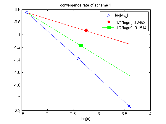
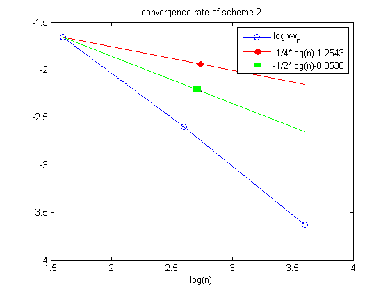
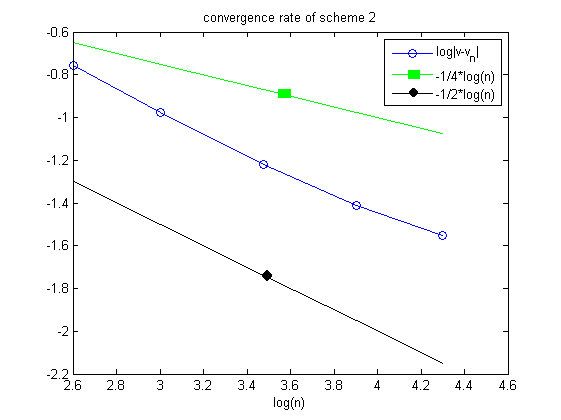
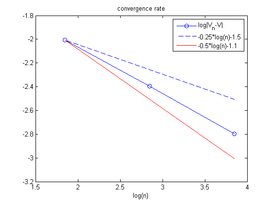
Our numerical results in the next section suggest that the order of convergence we predicted is better than we prove here. In fact, the constant multiplying the power of $n$ is small, which we think is due to the fact that we have a very efficient way of calculating conditional expectations. We will leave the investigation of this phenomena for future research.

5 Numerical examples

In the first subsection we consider two toy models, which are variations of geometric Brownian motion, the first one with capped coefficients and the other one with absorbing boundaries. In Subsections 5.2, we consider the CEV model and in 5.3, we consider the CIR model. In Subsection 5.4 we consider the European capped barrier of [11] and its American counterpart. We close the paper by considering another modification of geometric Brownian motion with discontinuous coefficients, see Subsection 5.5. In these sections we report the values of the option prices, optimal exercise boundaries, the time/accuracy performance of the schemes and numerical convergence rates. All computations are implemented in Matlab R2014a on Intel(R) Core(TM) i5-5200U CPU @2.20 GHz, 8.00 GB installed RAM PC.

5.1 Approximation of one dimensional diffusion with bounded $\mu$ and $\sigma$ by using both two schemes

We consider the following model:

(5.1) $$dS_{t}=[(A_{1}\wedge S_{t})\vee B_{1}]dt+[(A_{2}\wedge S_{t})\vee B_{2}]dW_{t},\quad S_{0}=x,$$

where $A_{1},B_{1},A_{2},B_{2}$ are constants, and the American put option with strike price $\$K$ and expiry date $T$:

(5.2) $$v(x)=\sup_{\tau\in\mathcal{T}_{[0,T]}}\mathbb{E}\left[e^{-r\tau}(K-S_{\tau})^{+}\right].$$

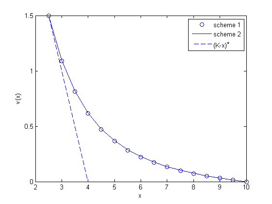
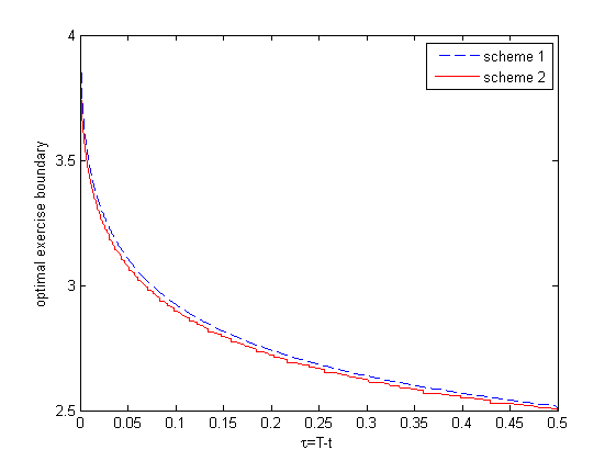
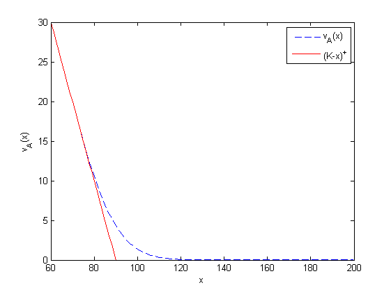
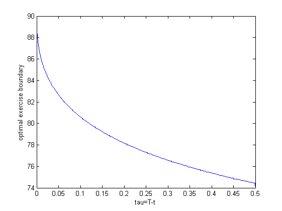
Figure 5.1 shows the value function $v$ and the optimal exercise boundary curve which we obtained using both schemes. Table LABEL:table:tm1 reports the schemes take and Figure 5.2 shows the rate of convergence of both models.

Figure 5.1: The left figure shows that value function of American put (5.2) under model (5.1) with parameters: $n=8000,r=0.1,K=4,A_{1}=10,A_{2}=10,B_{1}=2,B_{2}=2,T=0.5$. The right figure is the optimal exercise boundary curve. Here $\tau$ is the time to maturity.

Table 5.1: Put option prices(5.2) under model (5.1):

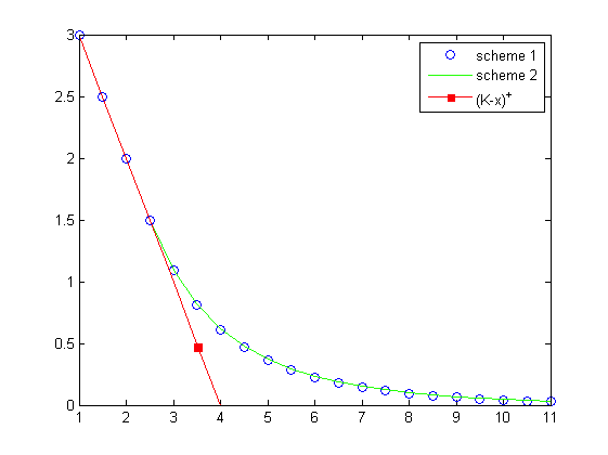
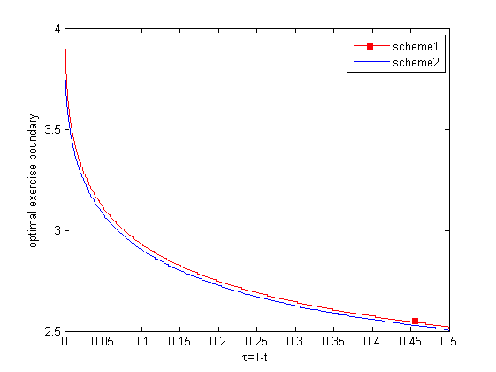
	scheme 1	scheme 2		scheme 1	scheme 2
n=1000	0.5954	0.6213	n=2000	0.6042	0.6213
error(%)	3.64	0.23	error(%)	2.21	0.08
CPU	0.540s	0.374s	CPU	2.097s	1.467s
	scheme 1	scheme 2		scheme 1	scheme 2
n=3000	0.6079	0.6214	n=4000	0.6100	0.6216
error(%)	1.61	0.06	error(%)	1.27	0.03
CPU	4.749s	3.249s	CPU	8.726s	5.747s
	scheme 1	scheme 2		scheme 1	scheme 2
n=5000	0.6114	0.6216	n=6000	0.6124	0.6216
error(%)	1.04	0.03	error(%)	0.88	0.02
CPU	14.301s	9.145s	CPU	24.805s	14.080s

Parameters used in computation are: $r=0.1,K=4,A_{1}=10,A_{2}=10,B_{1}=2,B_{2}=2,T=0.5,x=4$. Error is computed by taking absolute difference between $v_{n}(x)$ and $v_{30000}(x)$ and then dividing by $v_{30000}(x)$.

Figure 5.2: Convergence rate figure of both two schemes in the implement of American put (5.2) under (5.1). We draw $\log{|v-v_{n}|}\ vs\ \log{n}$ for both schemes to show the convergence speed. Here we pick $v(x)=v_{30000}(x)$ for $x=4$ and $n\in\{40,400,4000\}$. The slope of the left line given by linear regression is $-0.69981$, and the right is $-0.97422$. Parameters used in computation are: $r=0.1,K=4,A_{1}=10,A_{2}=10,B_{1}=2,B_{2}=2,T=0.5,x=4$.

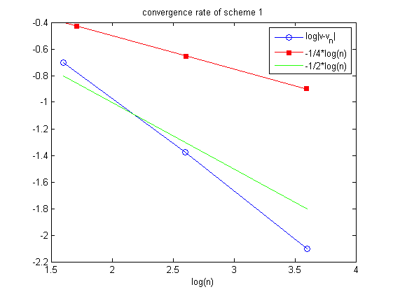
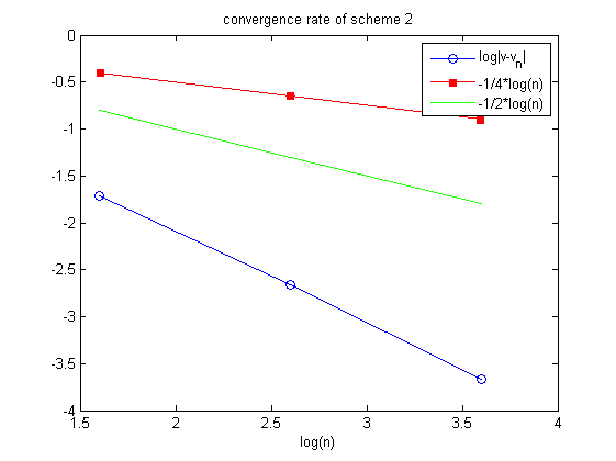
For comparison we will also consider a geometric Brownian motion with absorbing barriers. Let

(5.3) $$dY_{t}=Y_{t}dt+Y_{t}dW_{t},\quad Y_{0}=x,$$

and $B,C\in[-\infty,\infty)$ with $B<x<C$ and denote

(5.4) $$X_{t}=\mathbb{I}_{t<\inf\{s:Y_{s}\notin(B,C)\}}Y_{t}+\mathbb{I}_{t\geq\inf\{s:Y_{s}\notin(B,C)\}}Y_{\inf\{s:Y_{s}\notin(B,C)\}},\quad X_{0}=x.$$

As in the previous example, we show below the value function, times the schemes take and the numerical convergence rate.

Figure 5.3: The left figure shows the value function of American put (5.2) under model (5.4) with parameters: $n=30000,r=0.1,K=4,C=10,B=2,T=0.5$. The right figure is the optimal exercise boundary curve.

Figure 5.4: Convergence rate figure of both two schemes in the implement of American put (5.2) under (5.4). We draw $\log{|v-v_{n}|}\ vs\ \log{n}$ for both schemes to show the convergence speed. Here we pick, $v(x)=v_{30000}(x)$ for $x=4$ and $n\in\{40,400,4000\}$. The slope of the left line given by linear regression is $-0.74513$, the right one is $-0.98927$.

Table 5.2: put option prices(5.2) under (5.4)

	scheme 1	scheme 2		scheme 1	scheme 2
n=1000	0.5943	0.6175	n=2000	0.6029	0.6185
error(%)	3.44	0.24	error	2.05	0.09
CPU	0.240s	0.029s	CPU	0.667s	0.091s
	scheme 1	scheme 2		scheme 1	scheme 2
n=3000	0.6063	0.6184	n=4000	0.6082	0.6188
error(%)	1.49	0.09	error	1.17	0.03
CPU	1.220s	0.157s	CPU	1.927s	0.254s
	scheme 1	scheme 2		scheme 1	scheme 2
n=5000	0.6095	0.6188	n=6000	0.6104	0.6189
error(%)	0.96	0.04	error	0.81	0.02
CPU	2.720s	0.359s	CPU	3.723s	0.457s

Note: Parameters used in computation: $r=0.1,K=4,C=10,B=2,T=0.5,x=4$. Error is computed by taking absolute difference between $v_{n}(x)$ and $v_{30000}(x)$ and then dividing by $v_{30000}(x)$.

5.2 Pricing American put option under CEV

Set $\beta\leq 0$ and consider the CEV model:

(5.5) $$dS_{t}=rS_{t}+\delta S_{t}^{\beta+1}dW_{t},\quad S_{0}=x,$$

and let $\delta=\sigma_{0}x^{-\beta}$ (to be consistent with the notation of [11]). Consider the American put option pricing problem:

(5.6) $$v_{A}(x)=\sup_{\tau\in\mathcal{T}_{[0,T]}}\mathbb{E}\left[e^{-r\tau}(K-S_{\tau})^{+}\right].$$

Clearly, the CEV model given by (5.5) does not satisfies our assumptions. However, this limitation can be solved by truncating the model. The next result shows that if we choose absorbing barriers $B,C>0$ such that $B$ is small enough and $C$ is large enough, then the optimal stopping problem does not change much. Hence, we can apply our numerical scheme for the absorbed diffusion and still get error estimates of order $O(n^{-1/4})$.

Lemma 5.1.

Choose $0<B<C$. Consider the CEV model given by (5.5) and let $X$ be the absorbed process

$$X_{t}=\mathbb{I}_{t<\inf\{s:S_{s}\notin(B,C)\}}S_{t}+\mathbb{I}_{t\geq\inf\{s:S_{s}\notin(B,C)\}}S_{\inf\{s:S_{s}\notin(B,C)\}},\ \ t\geq 0.$$

Then

(5.7) $$\sup_{\tau\in\mathcal{T}_{[0,T]}}\mathbb{E}[e^{-r\tau}(K-S_{\tau})^{+}]-\sup_{\tau\in\mathcal{T}_{[0,T]}}\mathbb{E}[e^{-r\tau}(K-X_{\tau})^{+}]=\mathbb{I}_{\tau^{*}\leq\tau_{B}}B+O(C^{-k}),\ \ \forall k\geq 1,$$

where $\tau^{*}$ is the optimal time for first the expression on the left and $\tau_{B}$ is the first time $S_{t}$ is below the level $B$.

Proof.

Let us briefly argue that $\mathbb{E}\left(\max_{0\leq t\leq T}S^{k}_{t}\right)<\infty$ for all $k$. Clearly, if $\beta=0$ then $S$ is a geometric Brownian motion and so the statement is clear. For $\beta<0$ we observe that the process $Y=S^{-\beta}$ belongs to CIR family of diffusions (see equation (1) in [14]). Such process can be represented in terms of BESQ (squared Bessel processes); see equation (4) in [14]. Finally, the moments of the running maximum of the (absolute value) Bessel process can be estimated by Theorem 4.1 in [15]. Hence from the Markov inequality it follows that $\mathbb{P}(\max_{0\leq t\leq T}S_{t}\geq M)=O(M^{-k}).$ Next, consider the stopping time $\tau_{B}=\inf\{t:S_{t}=B\}\wedge T$. If $\tau_{B}<T$ then the payoff of the put option is $K-B$, and since $S$ is non–negative its $B$ optimal to stop at this time. It is clear also that one would make no error if $B$ is always in the stopping region.

Table 5.3: Pricing American puts (5.6) under the CEV (5.5) model with different $\beta$’s by using the first scheme

$K$	$\beta=-1$	$\beta=-\frac{1}{3}$
90	1.4373(1.5122)	1.3040(1.3844)
100	4.5359(4.6390)	4.5244(4.6491)
110	10.6502(10.7515)	10.7716(10.8942)

Parameters used in computation are: $\sigma_{0}=0.2,x=100,T=0.5,r=0.05,n=15000,B=0.01,C=200$. The values in the parentheses are the results from last row of Tables $4.1,4.2,4.3$ from paper [29], which carries out the artificial boundary method discussed in the introduction. This is a finite difference method which relies on artificially introducing an exact boundary condition.

Table 5.4: Prices of the American puts (5.6) under (5.5) with different $\beta$’s by using the second scheme

$K$	$\beta=-1$	$\beta=-\frac{1}{3}$
90	1.5123(1.5122)	1.3845(1.3844)
100	4.6392(4.6390)	4.6492(4.6489)
110	10.7517(10.7515)	10.8943(10.8942)

Parameters used in computation are: $\sigma_{0}=0.2,x=100,T=0.5,r=0.05,n=15000,B=0.01,C=200$. The values in the parentheses are the results from last row of Tables $4.1,4.2,4.3$ from paper [29], which carries out the artificial boundary method discussed in the introduction. This is a finite difference method which relies on artificially introducing an exact boundary condition.

Figure 5.5: The left figure shows that value function of American put (5.6) under CEV (5.5) with parameters: $n=2000,\beta=-\frac{1}{3},\delta=\sigma_{0}(100)^{-\beta},\sigma_{0}=0.2,T=0.5,r=0.05,B=0.01,C=200,K=90.$ The right figure is the optimal exercise boundary curve which $\tau=T-t$ denotes time to maturity. With these parameters $F(60)=-0.3243,F(70)=0.1790$ (where $F$ is defined in (5.8)), from which we conclude that the unique root is in (60,70). So there in fact is no error in introducing a lower barrier. In this case $b=9.3577$ (where $b$ is defined in (5.9)).

Since we observed that second scheme exhibits faster convergence, we report the CPU time and errors for second scheme.

Table 5.5: Prices of the American puts under (5.5) with different $beta$’s (second scheme)

	$\beta=-1$	$\beta=-\frac{1}{3}$
K=90	1.5147	1.3862
CPU	0.335s	0.259s
error(%)	0.16	0.12
K=100	4.6414	4.6383
CPU	0.314s	0.256s
error(%)	0.05	0.23
K=110	10.7523	10.8925
CPU	0.338s	0.253s
error(%)	0.005	0.02

Parameters used in computation are: $\sigma_{0}=0.2,x=100,T=0.5,r=0.05,B=0.01,C=200$. The Error is computed by taking absolute difference between $v_{n}(x)$ and $v_{15000}(x)$ and then dividing by $v_{15000}(x)$.

Table 5.6: Pricing American puts (5.6) under (5.5) with different $\sigma_{0}$ (second scheme)

	$\sigma_{0}=0.2$	$\sigma_{0}=0.3$	$\sigma_{0}=0.4$
K=35	1.8606(1.8595)	4.0424(4.0404)	6.4017(6.3973)
CPU	0.247s	0.171s	0.136s
error(%)	0.04	0.03	0.06
K=40	3.3965(3.3965)	5.7920(5.7915)	8.2584(8.2574)
CPU	0.237s	0.172s	0.154s
error(%)	0.01	0.002	0.004
K=45	5.9205(5.9204)	8.1145(8.1129)	10.5206(10.5167)
CPU	0.203s	0.170s	0.146s
error(%)	0.01	0.02	0.03

Parameters used in computation are: $T=3,r=0.05,x=40,\beta=-1,n=100,B=0.01,C=100$. Error is computed by taking absolute difference between $v_{n}(x)$ and $v_{30000}(x)$ and then dividing by $v_{30000}(x)$. The values in the parentheses are the results computed by FDM:$1024\times 1024$ reported in Table 1 of [30].

In Table 5.6 we compare our numerical results with the ones reported in Table 1 of [30], the numerical values here are closer to results computed by FDM:$1024\times 1024$, which is the traditional Crank-Nicolson finite difference scheme (the $1024\times 1024$ refer to the size of the lattice). The CPU time of FDM:$1024\times 1024$ is 6.8684s. Table 1 of [30] also reports the performance of the Laplace-Carson transform and the artificial boundary method of [29] (both of which we briefly described in the introduction). The CPU for Laplace-Carson method is 0.609s, ABC:$512\times 512$ is 0.9225s. If we consider FDM:$1024\times 1024$ as a Benchmark, our method is more than 30 times faster with accuracy up to 4 decimal points. Comparing with ABC:$512\times 512$ method, our method is about 5 times faster with the same accuracy. Our method is about 3 times faster than what the Laplace transform method produced when it had accuracy up to 3 decimal points. (Here accuracy represents the absolute difference between the computed numerical values and the FDM:$1024\times 1024$ divided by the FDM:$1024\times 1024$).

5.3 Pricing American put option under CIR

In this subsection, we use numerical scheme to evaluate American put options $v_{A}(x)$ (recall formula (5.6)) under CIR model. (This model is used for pricing VIX options, see e.g. [23]). Let the volatility follow

(5.10) $$dY_{t}=(\beta-\alpha Y_{t})dt+\sigma\sqrt{Y_{t}}dW_{t},\quad Y_{0}=y,$$

Consider the absorbed process

$$X_{t}=\mathbb{I}_{t<\inf\{s:Y_{s}\notin(B,C)\}}Y_{t}+\mathbb{I}_{t\geq\inf\{s:Y_{s}\notin(B,C)\}}Y_{\inf\{s:Y_{s}\notin(B,C)\}},\quad t\geq 0,$$

for $0<B<C$. Same arguments as in Section 5.2 give that for CIR process $\mathbb{P}(\max_{0\leq t\leq T}Y_{t}\geq C)=O(C^{-k})$, $k\geq 1$. Moreover, from Theorem 2 in [14] it follows that $\mathbb{P}(\min_{0\leq t\leq T}Y_{t}\leq B)=O(B^{2\nu})$ for $\nu=\frac{2\beta}{\sigma^{2}}-1>0$. Thus if we consider the absorbed diffusion $X$ then the change of the value of the option price is bounded by $O(C^{-k})+O(B^{2\nu})$ for all $k$. (In fact, potentially we do not make any error by having an absorbing boundary if $B$ is small enough, as we argued in the previous section.)

Table 5.7: Prices of American puts (5.6) under (5.10) with different $K$

	scheme 1	scheme 2
$K=35$	4.4654	4.5223
$K=40$	8.1285	8.1932
$K=45$	12.4498	12.5167

Parameters used in computation are: $\sigma=2,y=40,T=0.5,r=0.1,B=0.01,C=200,\beta=2,\alpha=0.5,n=30000$.

As the previous example, since the second scheme looks more efficient, we only report its time with the accuracy performance here.

Table 5.8: American put prices under (5.10) for a variety of $K$’s using the second scheme

	$K=35$	$K=40$	$K=45$
$n=100$	4.5140	8.1834	12.5127
CPU	0.245s	0.202s	0.198s
error(%)	0.18	0.12	0.03
$n=500$	4.5215	8.1918	12.5163
CPU	0.600s	0.585s	0.579s
error(%)	0.02	0.02	0.003
$n=1000$	4.5238	8.1925	12.5170
CPU	0.807s	0.813s	0.839s
error(%)	0.03	0.01	0.002

Parameters used in computation are: $\sigma=2,y=40,T=0.5,r=0.1,B=0.01,C=200,\beta=2,\alpha=0.5$. Error is computed by taking absolute difference between $v_{n}(x)$ and $v_{30000}(x)$ and then dividing by $v_{30000}(x)$.

5.4 Pricing double capped barrier options under CEV by using second scheme

In this subsection, we use second scheme to evaluate double capped barrier call options under the CEV model given by (5.5). Let us denote the European option value by

(5.11) $$v_{E}(x)=e^{-rT}\mathbb{E}\left[\mathbb{I}_{T<\tau^{*}}(S_{T}-K)^{+}\right],$$

and the American option value by

(5.12) $$v_{A}(x)=\sup_{\tau\in\mathcal{T}_{[0,T]}}\mathbb{E}\left[\mathbb{I}_{\tau<\tau^{*}}e^{-r\tau}(S_{\tau}-K)^{+}\right],$$

where $\tau^{*}=\inf\{t\geq 0;S_{t}\neq(L,U)\}$. We use the parameters values given in [11] and report our results in Table 5.10 and Figure 5.6.

Table 5.9: Double capped European Barrier Options (5.11) under CEV(5.5) (second scheme)

$U$	$L$	$K$	$\beta=-0.5$	$\beta=0$	$\beta=-2$	$\beta=-3$
120	90	95	1.9012	1.7197	2.5970	3.2717
	CPU		0.970s	1.026s	6.203s	1.209s
	error		0.96%	1.2%	0.4%	2.7%
120	90	100	1.1090	0.9802	1.6101	2.0958
	CPU		0.957s	1.102s	6.066s	1.205s
	error		0.98%	1.2%	0.44%	2.3%
120	90	105	0.5201	0.4473	0.8142	1.1072
	CPU		0.961s	1.023s	6.205s	1.187s
	error		1.00%	1.3%	0.53%	2.2%
	n		2000	2000	5000	2000

Table 5.10: Double capped American Barrier Options (5.12) under CEV(5.5) (second scheme)

$U$	$L$	$K$	$\beta=-0.5$	$\beta=0$	$\beta=-2$	$\beta=-3$
120	90	95	9.8470	9.8271	9.9826	10.0586
	CPU		0.965s	1.007s	1.248s	1.170s
	error		0.55%	0.63%	0.56%	0.81%
120	90	100	7.4546	7.4522	7.5118	7.5203
	CPU		0.942s	1.017s	1.239s	1.211s
	error		0.70%	0.8%	0.47%	0.57%
120	90	105	5.2612	5.2788	5.2345	5.1669
	CPU		0.968s	1.044s	1.145s	1.188s
	error		1.00%	1.2%	0.35%	0.17%
	n		2000	2000	2000	2000

Parameters used in calculations are: $x=100,\sigma(100)=0.25$ (denoting $\sigma(S)=\delta S^{1+\beta}$), $r=0.1,T=0.5$. Error is computed by taking the absolute difference between $v_{n}$ and $v_{40000}$ and then dividing by $v_{40000}$.

Figure 5.6: The left figure shows the value function $v_{A}(x)$(5.12) and $v_{E}(x)$(5.11) with Parameters: $\delta=2.5,r=0.1,T=0.5,\beta=-0.5,n=5000,L=90,U=120,K=100$,. In the right figure, we show the $\log{|v-v_{n}|}$ vs $\log{n}$ picking $v(x)=v_{40000}(x)$, $x=100$, and $n\in\{400,1000,3000,8000,20000\}$. The slope of the blue line given by linear regression is $-0.47178$.

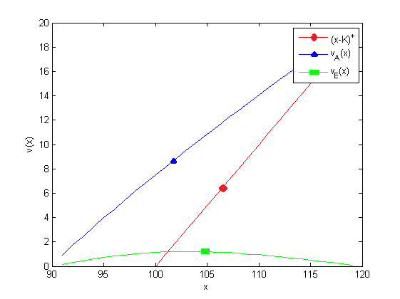
5.5 Pricing double capped American barrier options with jump volatility by using second scheme

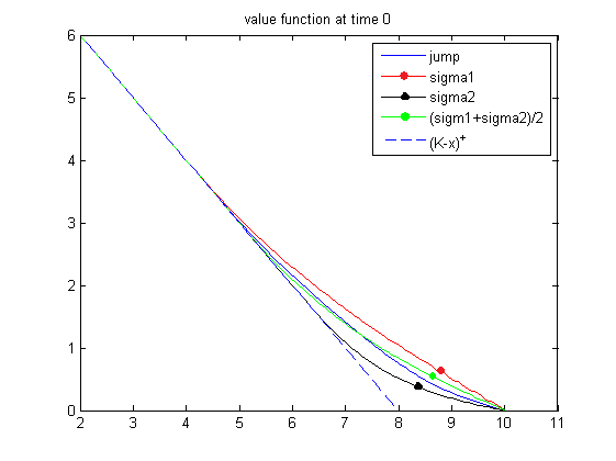
In this subsection, we show the numerical results for pricing double capped American barrier option when the volatility has a jump. Consider the following modification of a geometric Brownian motion:

(5.13) $$dS_{t}=rS_{t}dt+\sigma(S_{t})S_{t}dW_{t},S_{0}=x$$

where $\sigma(S_{t})=\sigma_{1}$, for $S_{t}\in[0,S_{1}]$, $\sigma(S_{t})=\sigma_{2}$, for $S_{t}\in[S_{1},\infty)$. We will compute the American option price

(5.14) $$v(x)=\sup_{\tau\in\mathcal{T}_{[0,T]}}\mathbb{E}\left[e^{-r\tau}\mathbb{I}_{\tau<\tau^{*}}(S_{\tau}-K)^{+}\right],$$

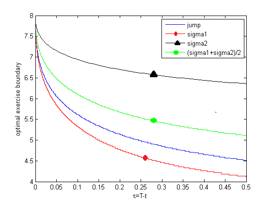
where $\tau^{*}=\inf\{t\geq 0;S_{t}\neq(L,U)\}$. We use scheme 2 here, since it can handle discontinuous coefficients; see Figures 5.7 and 5.8. We compare it to the geometric Brownian motion (gBm) problem with different volatility parameters. In particular, we observe that although the jump model’s price and the gBm model with average volatility are close in price, the optimal exercise boundaries differ significantly.

Figure 5.7: There are four curves in the left figure. They are value functions (5.14) under model (5.13) with different values of $\sigma(S_{t})$ as specified in the legend. The parameters used in computations are: $n=4000,r=0.1,S_{1}=K=8,L=2,U=10,\sigma_{1}=0.7,\sigma_{2}=0.3,T=0.5$. Here $\sigma_{2}<\frac{\sigma_{1}+\sigma_{2}}{2}<\sigma_{1}$, and as expected the gBm option price decreases as $\sigma$ decreases but the gBm price with jump volatility and one corresponding to gBm with $\sigma=\sigma_{2}$ intersect in the interval $[7,8]$. The right figure is of the optimal exercise boundary curves.

Figure 5.8: Convergence rate figure of scheme 2 in the implement of double capped American put (5.14) under (5.13). We pick $v(x)=v_{40000}(x)$ to be the actual price, and the other three values are $v_{70}(x),v_{700}(x),v_{7000}(x),x=8$. The slope of the blue line given by linear regression approach is $-0.39499$. Parameters used in computation: $n=4000,r=0.1,K=8,L=2,U=10,\sigma_{1}=0.7,\sigma_{2}=0.3,S1=8,T=0.5$.

References

- [1] S. Ankirchner, T. Kruse, and M. Urusov, A functional limit theorem for irregular SDEs, To appear in Annales de l’Institut Henri Poincaré - Probabilités et Statistiques.
- [2] S. Ankirchner, T. Kruse, and M. Urusov, Numerical approximation of irregular SDEs via Skorokhod embeddings, J. Math. Anal. Appl., 440 (2016), pp. 692–715.
- [3] S. r. Asmussen and P. W. Glynn, Stochastic simulation: algorithms and analysis, vol. 57 of Stochastic Modelling and Applied Probability, Springer, New York, 2007.
- [4] D. Baños, T. Meyer-Brandis, F. Proske, and S. Duedahl, Computing deltas without derivatives, Finance Stoch., 21 (2017), pp. 509–549.
- [5] N. Bäuerle and E. Bayraktar, A note on applications of stochastic ordering to control problems in insurance and finance, Stochastics, 86 (2014), pp. 330–340.
- [6] E. Bayraktar, On the perpetual American put options for level dependent volatility models with jumps, Quantitative Finance, 11 (2011), pp. 335–341.
- [7] E. Bayraktar and A. Fahim, A stochastic approximation for fully nonlinear free boundary parabolic problems, Numer. Methods Partial Differential Equations, 30 (2014), pp. 902–929.
- [8] D. S. Clark, Short proof of a discrete Gronwall inequality, Discrete Appl. Math., 16 (1987), pp. 279–281.
- [9] J. C. Cox, The Constant Elasticity of Variance Option Pricing model, Journal of Portfolio Management, 22 (1996), pp. 15–17.
- [10] J. C. Cox, J. E. Ingersoll, Jr., and S. A. Ross, A theory of the term structure of interest rates, Econometrica, 53 (1985), pp. 385–407.
- [11] D. Davydov and V. Linetsky, Pricing and Hedging Path-Dependent Options Under the CEV Process, Management Science, 47 (2001), pp. 949–965.
- [12] Y. Dolinsky and K. Kifer, Binomial approximations for barrier options of Israeli style, Advances in Dynamic Games, 11 (2011), pp. 447–469.
- [13] P. Glasserman, Monte Carlo methods in financial engineering, vol. 53 of Applications of Mathematics (New York), Springer-Verlag, New York, 2004. Stochastic Modelling and Applied Probability.
- [14] A. Göing-Jaeschke and M. Yor, A survey and some generalizations of Bessel processes, Bernoulli, 9 (2003), pp. 313–349.
- [15] S. E. Graversen and G. Peskir, Maximal inequalities for Bessel processes, J. Inequal. Appl., 2 (1998), pp. 99–119.
- [16] U. Gruber and M. Schweizer, A diffusion limit for generalized correlated random walks, J. Appl. Probab., 43 (2006), pp. 60–73.
- [17] S. D. Jacka, Optimal stopping and the American put, Mathematical Finance, 1 (1991), pp. 1–14.
- [18] I. Karatzas, On the pricing of American options, Appl. Math. Optim., 17 (1988), pp. 37–60.
- [19] I. Karatzas and S. E. Shreve, Brownian motion and stochastic calculus, vol. 113 of Graduate Texts in Mathematics, Springer-Verlag, New York, 1988.
- [20] K. Kifer, Game Options, Finance and Stochastics, 4 (2000), pp. 443–463.
- [21] , Error Estimates for Binomial Approximations of Game Options, Annals of Applied Probability, 18 (2006), pp. 1737–1770.
- [22] Y. Kifer, Dynkin games and Israeli options, ISRN Probability and Statistics, (2013).
- [23] Y. Kitapbayev and J. Detemple, On American VIX options under the generalized 3/2 and 1/2 models, ArXiv e-prints, (2016).
- [24] D. Lamberton and L. C. G. Rogers, Optimal stopping and embedding, J. Appl. Probab., 37 (2000), pp. 1143–1148.
- [25] F. A. Longstaff and E. S. Schwartz, Valuing American Options by Simulation: A Simple Least-Squares approach, The Review of Financial Studies, 14 (2001), p. 113.
- [26] Y. Ohtsubo, Optimal stopping in sequential games with or without a constraint of always terminating, Math. Oper. Res., 11 (1986), pp. 591–607.
- [27] G. Peskir and A. Shiryaev, Optimal stopping and free-boundary problems, Lectures in Mathematics ETH Zürich, Birkhäuser Verlag, Basel, 2006.
- [28] P. Wilmott, S. Howison, and J. Dewynne, The mathematics of financial derivatives, Cambridge University Press, Cambridge, 1995. A student introduction.
- [29] H. Y. Wong and J. Zhao, An artificial boundary method for American option pricing under the CEV model, SIAM J. Numer. Anal., 46 (2008), pp. 2183–2209.
- [30] , Valuing American options under the CEV model by Laplace-Carson transforms, Oper. Res. Lett., 38 (2010), pp. 474–481.