BEC polaron in harmonic trap potentials in the weak coupling regime: Lee-Low-Pines-type approach

Abstract

We have calculated the zero-temperature binding energy of a single impurity atom immersed in a Bose-Einstein condensate (BEC) of ultracold atoms. The impurity and the condensed atoms are trapped in the respective axially symmetric harmonic potentials, where the impurity interacts with bosonic atoms in the condensate via low-energy $s$-wave scattering. In this case, bosons are excited around the impurity to form a quasiparticle, namely, a BEC polaron. We have developed a variational method, a la Lee-Low-Pines (LLP), for description of the polaron that has a conserved angular momentum around the symmetric axis. We find from numerical results that the binding between the impurity and the excited bosons breaks the degeneracy of the impurity energy with respect to the total angular momentum of the polaron. The angular momentum is partially shared by the excited bosons in a manner that is similar to the drag effect on the polaron momentum by a phonon cloud in the LLP theory for the electron-phonon system.

I Introduction

Polarons originally meant electrons dressed by locally excited phonons, which comprise one of the elementary excitations in ionic crystals. These excitations provide a widely applicable physics concept for quasiparticles in various environmental media Landau1 ; FPZ1 ; Mahan1 ; polaronreview1 ; LLP1 . Recently, many-body systems of trapped ultracold atoms allow us to access the properties of such quasiparticles in a clean and controlled manner. Examples include studies on Bose-Einstein condensate (BEC) and Fermi polarons that are impurity atoms immersed in Bose-Einstein condensed atoms Cucchietti1 ; Sacha1 ; Tempere1 ; Casteels1 ; Rath1 ; Shashi1 ; Levinsen2 ; Dehkharghani5 ; Ardila2 ; Yin1 ; Christensen1 ; Vlietinck1 ; Grusdt1 ; Grusdt3 ; Shchadilova1 and degenerate Fermi atoms Chevy1 ; Schirotzek1 ; Schmidt1 ; Kohstall1 ; Koschorreck1 ; Vlietinck2 ; Massignan1 ; Yi1 , respectively, as well as on polarons in optical lattices Bruderer1 . Experimental realizations of BEC polarons were achieved first in a weak coupling regime Catani1 ; Scelle1 ; Hohmann1 . Then, recent experiments in a strong coupling regime around the unitary limit have observed a behavior of the binding energy between an impurity and excited bosons in the BEC via radio frequency (RF) spectroscopy and in-situ imaging technology Jrgensen1 ; Hu1 . These results show a smooth crossover from a weak mean-field to a strong molecular regime. In these experiments, a number of bosonic atoms are optically trapped to form a BEC, while an impurity atom immersed in the condensate starts to interact with bosons. Consequently, a polaron, i.e., an impurity accompanied by locally excited bosons, is formed. The interaction between the impurity and bosons is characterized by an $s$-wave scattering length for low energy dynamics, while its sign and strength can be tuned by the Feshbach resonance from a weak- to a strong-coupling regime. The RF spectroscopy measures the energy shift between hyperfine states of the impurity due to the interaction, which corresponds to the binding (interaction) energy of the polaron.

These experimental results for the BEC polarons are as a whole in agreement with theoretical predictions, which have been so far obtained entirely for spatially uniform systems. However, the real systems are in optical traps, which are well described by harmonic oscillator potentials. In the present study we investigate the properties of a BEC polaron in the case in which a single impurity atom and Bose condensed atoms are put in the respective axially symmetric harmonic potentials in three dimensions and interact attractively with each other in a regime where the coupling is weak or even intermediate, but is still far away from the unitarity. Since the axial component of the total angular momentum of the system is conserved in such axially symmetric potentials, we focus on how the polaron’s binding energy depends on a given total angular momentum of the impurity and excited bosons. We also figure out detailed physics, such as a drag effect by excited bosons, that underlies the mean-field result in the trapped systems, although the mean-field result is occasionally referred to as a reference theory at weak coupling.

This paper is organized as follows: In Sec. II we present the low energy effective Hamiltonian for a single impurity atom and bosons in axially symmetric harmonic potentials, and, by assuming that most of the bosons are in a BEC, i.e., at the lowest energy level, implement the Bogoliubov approximation to obtain a Yukawa-type interaction between the impurity and excited bosons. In Sec. III, for the state of the immersed impurity specified in terms of the harmonic oscillator eigenstates, we employ a variational method, a la Lee-Low-Pines (LLP) LLP1 , to obtain the ground state of a polaron under fixed total angular momentum around the symmetric axis. In Sec. IV, we present numerical results for the properties of polarons in various states by utilizing the parameter values that are used in experiments. The last section is devoted to summary and outlooks.

II Effective Hamiltonian

We consider a zero-temperature atomic many-body system of bosons and an impurity that are trapped in axially symmetric harmonic potentials in three dimensions. First, bosonic atoms (denoted bya symbol ‘$b$’) are condensed in the lowest energy level, and then a single impurity atom is introduced to interact attractively with bosons. Here we assume that the impurity is a fermion (denoted by a symbol ‘$f$’) for later convenience. A low-energy effective Hamiltonian for such a system is given by

$$\mathcal{H}_{eff}\left({\bf r}\right) = H_{ho}^{f}\left({\bf r}\right)+\int_{{\bf r}^{\prime}}\phi^{\dagger}({{\bf r}^{\prime}})\left[H_{ho}^{b}\left({\bf r}^{\prime}\right)+g\delta^{(3)}({\bf r}-{\bf r}^{\prime})\right]\phi({{\bf r}^{\prime}})$$ (1)

$$= H_{ho}^{f}\left({\bf r}\right)+\sum_{s}E_{s}^{b}b_{s}^{\dagger}b_{s}+g\sum_{s,s^{\prime}}\phi_{s}^{b}\left({\bf r}\right)^{*}\phi_{s^{\prime}}^{b}\left({\bf r}\right)b_{s}^{\dagger}b_{s^{\prime}},$$ (2)

$$H_{ho}^{b,f}\left({\bf r}\right) = \frac{1}{2m_{b,f}}\left(p_{z}^{2}+p_{r}^{2}+\frac{L_{z}^{2}}{r^{2}}\right)+\frac{m_{b,f}\omega_{bt,ft}^{2}}{2}r^{2}+\frac{m_{b,f}\omega_{b,f}^{2}}{2}z^{2},$$ (3)

where $p_{z}^{2}\equiv-\frac{\partial^{2}}{\partial z^{2}},\,p_{r}^{2}\equiv-\frac{1}{r}\frac{\partial}{\partial r}r\frac{\partial}{\partial r},\,L_{z}\equiv-i\frac{\partial}{\partial\varphi}$ is the angular momentum operator around the $z$ axis (the axial symmetry holds around the $z$ axis), ${\bf r}=\left(r,\varphi,z\right)$ is the cylindrical coordinate of the impurity, $\omega_{b}\left(\omega_{f}\right)$ and $\omega_{bt}\left(\omega_{ft}\right)$ are the frequencies of the harmonic potentials in $z$ and radial $r$ directions, respectively, for bosons (impurity), and $g=\frac{2\pi a_{bf}}{m_{r}}$ is the coupling constant between the boson and the impurity given in terms of an $s$-wave scattering length $a_{bf}$, which is assumed to be negative and short, and the reduced mass $m_{r}=\frac{m_{b}m_{f}}{m_{b}+m_{f}}$ with $m_{b}$ ($m_{f}$) being the mass of boson (impurity) PethickSmith1 . We have ignored a possible boson-boson interaction, which would not bring qualitative changes in the present study as long as it is repulsive and so weak that the interaction energy is smaller than the trap frequency. In the case of relatively strong boson-boson interactions, i.e., $N_{0}a_{bb}/\bar{a}\gg 1$ where $N_{0}$ is the number of condensed bosons, $a_{bb}$ the boson-boson scattering length, and $\bar{a}$ the averaged harmonic amplitude PethickSmith1 , the condensate of trapped bosons is well described by semi-classical approximations such as the Thomas-Fermi approximation, while low energy excitations upon it become collective modes that still have discrete quantum numbers associated with symmetries of the system Dalfovo1 ; Pitaevskii1 . In contrast, the boson sector in our system with $a_{bb}=0$ is, for any state, in the quantum regime. No semi-classical approximation is thus relevant, which allows us to easily examine how excited bosons with definite quantum numbers distribute around the impurity as will be seen later. As for the relevance to possible experiments, the present system is not necessarily academic, but vanishing $a_{bb}$ can be realized experimentally, e.g., for rubidium isotopes ⁸⁵Rb and ⁸⁷Rb, by using the Feshbach resonance abb1 ; abb2 , while the boson-impurity scattering length is left finite. It is also noted that the Bose collapse, not desired in this study, is prevented by the zero point energy in trap potentials even for negative $a_{bb}$ as long as it is sufficiently small Mueller1 .

We have used the second quantized representation only for bosons, and expanded the boson field operator $\phi\left({\bf r}\right)$ in terms of the harmonic potential eigenfunctions $\phi_{s}^{b}\left({\bf r}\right)$:

$$\phi\left({\bf r}\right) = \sum_{s}\phi_{s}^{b}\left({\bf r}\right)b_{s},$$ (4)

where $s$ denotes the quantum number of the eigenstate whose single particle energy is given by $E_{s}^{b}$, and $b_{s}$ ($b_{s}^{\dagger}$) is the corresponding annihilation (creation) operator. The explicit representation of a set of the quantum numbers will be given just below. We employ the abbreviation $\int_{\bf r}\equiv\int_{-\infty}^{\infty}{\rm d}z\int_{0}^{\infty}{\rm d}rr\int_{0}^{2\pi}{\rm d}\varphi$ and the unit in which $\hbar=1$ throughout the paper.

II.1 Bogoliubov-type approximation

Since most of the bosons are in a BEC in the case of weak coupling and zero temperature, we implement the Bogoliubov-type approximation for the effective Hamiltonian, i.e., only interaction processes involving the condensed bosons are taken into account:

$$\mathcal{H}_{eff}\simeq\mathcal{H} = H_{ho}^{f}\left({\bf r}\right)+E_{0}^{b}N_{0}+gN_{0}|\phi_{0}^{b}({\bf r})|^{2}$$ (5)

$$+\sum_{s\neq 0}E_{s}^{b}b_{s}^{\dagger}b_{s}+g\sqrt{N_{0}}\sum_{s\neq 0}\left[\phi_{0}^{b}({\bf r})^{*}\phi_{s}^{b}({\bf r})b_{s}+\phi_{s}^{b}({\bf r})^{*}\phi_{0}^{b}({\bf r})b_{s}^{\dagger}\right],$$

where $s=0$ denotes the lowest energy level at which the bosons are condensed, and $b_{0},b_{0}^{\dagger}\simeq\sqrt{N_{0}}$, with $N_{0}$ being the number of the condensed bosons. We then express the Hamiltonian explicitly as

$${\mathcal{H}} = \frac{1}{2m_{f}}\left(p_{z}^{2}+p_{r}^{2}+\frac{L_{z}^{2}}{r^{2}}\right)+\frac{m_{f}\omega_{ft}^{2}}{2}r^{2}+\frac{m_{f}\omega_{f}^{2}}{2}z^{2}+E_{0}^{b}N_{0}+gN_{0}|\phi_{0,0,0}^{b}(r,\varphi,z)|^{2}$$ (6)

$$+{\sum_{n,n_{t},m}}^{\prime}E_{n,n_{t}}^{b}b_{n,n_{t},m}^{\dagger}b_{n,n_{t},m}$$

$$+g\sqrt{N_{0}}{\sum_{n,n_{t},m}}^{\prime}\left[\Phi_{n,n_{t},m}(r,z)e^{im\varphi}b_{n,n_{t},m}+\Phi_{n,n_{t},m}^{*}(r,z)e^{-im\varphi}b_{n,n_{t},m}^{\dagger}\right],$$

where the eigenenergies and eigenfunctions with a normalization factor ${\mathcal{N}}$ for free bosons are given by

$$E_{n,n_{t}}^{b} = \omega_{b}\left(n+\frac{1}{2}\right)+\omega_{bt}\left(n_{t}+1\right),$$ (7)

$$\phi_{n,n_{t},m}^{b}({\bf r}) = {\mathcal{N}}e^{im\varphi}\Psi_{n_{t},|m|}^{b}(r)\Psi_{n}^{b}(z)$$ (8)

with the eigenfunctions in $z$ and radial directions Bethe1 ,

$$\Psi_{n}^{b}(z) \equiv e^{-\frac{m_{b}\omega_{b}}{2}z^{2}}H_{n}\left(\sqrt{m_{b}\omega_{b}}z\right),$$ (9)

$$\Psi_{n_{t},|m|}^{b}(r) \equiv r^{|m|}e^{-\frac{m_{b}\omega_{bt}}{2}r^{2}}\frac{\left(\frac{n_{t}-|m|}{2}\right)!\Gamma\left(|m|+1\right)}{\Gamma\left(|m|+1+\frac{n_{t}-|m|}{2}\right)}L_{\frac{n_{t}-|m|}{2}}^{\left(|m|\right)}\left(m_{b}\omega_{bt}r^{2}\right),$$ (10)

given in terms of the Hermite and Laguerre polynomials, $H_{n}(x)$ and $L_{n}^{(k)}(x)$, respectively. The primary quantum numbers in $z$ and radial directions are given by $n=0,1,2,\cdots$ and $n_{t}=0,1,2,\cdots$, respectively, and the energy level $E_{n,n_{t}}^{b}$ is degenerate for the eigenvalues of $L_{z}$: $|m|=n_{t},n_{t}-2,n_{t}-4,\cdots,1\,\mbox{ or }\,0$. We have also defined

$$\Phi_{n,n_{t},m}(z,r) \equiv e^{-im\varphi}\phi_{n,n_{t},m}^{b}({\bf r})\phi_{0,0,0}^{b}({\bf r})^{*},$$ (11)

and its complex conjugate $\Phi_{n,n_{t},m}(z,r)^{*}$. Note that in the Hamiltonian (6) the symbol ${\sum_{n,n_{t},m}}^{\prime}$ denotes the summation over the boson’s eigenstates except $n=n_{t}=0$ which corresponds to the state of the BEC.

The eigenenergy and the corresponding eigenfunction of a bare (free) impurity in a state of $\left({\bar{n},\bar{n}_{t},\bar{m}}\right)$ determined by the harmonic potential are obtained by replacing the boson’s mass and frequencies in (7) and (8) with those of the impurity:

$$E_{\bar{n},\bar{n}_{t}}^{f} = \omega_{f}\left(n+\frac{1}{2}\right)+\omega_{ft}\left(n_{t}+1\right),$$ (12)

$$\phi_{\bar{n},\bar{n}_{t},\bar{m}}^{f}({\bf r}) = {\mathcal{N}}e^{i\bar{m}\varphi}\Psi_{\bar{n}_{t},|\bar{m}|}^{f}(r)\Psi_{\bar{n}}^{f}(z).$$ (13)

III Variational method a la LLP

We are interested in the ground state and low-lying excited states of a single impurity atom immersed in the BEC background, as dictated by the Hamiltonian (6). In order to construct a solution with the total angular momentum in the $z$ direction conserved, we first use a gauge transformation $S$, i.e., cranking of all bosons around the $z$ axis by $\varphi$, the angle of the impurity position Inglis1 ; Thouless1 ,

$$S = \exp\left(-i\varphi\sum_{n,n_{t},m}m\,b_{n,n_{t},m}^{\dagger}b_{n,n_{t},m}\right),$$ (14)

which transforms the operators as follows:

$$S^{-1}b_{n,n_{t},m}S = e^{-im\varphi}b_{n,n_{t},m},\quad S^{-1}b_{n,n_{t},m}^{\dagger}S=e^{im\varphi}b_{n,n_{t},m}^{\dagger},$$ (15)

$$S^{-1}\left(-i\partial_{\varphi}\right)S = -i\partial_{\varphi}-\sum_{n,n_{t},m}m\,b_{n,n_{t},m}^{\dagger}b_{n,n_{t},m}.$$ (16)

Thus, the transformed Hamiltonian reads

$$H^{\prime} \equiv S^{-1}\mathcal{H}S$$ (17)

$$= \frac{p_{r}^{2}}{2m_{f}}+\frac{1}{2m_{f}r^{2}}\left(-i\partial_{\varphi}-\sum_{n,n_{t},m}m\,b_{n,n_{t},m}^{\dagger}b_{n,n_{t},m}\right)^{2}+\frac{m_{f}\omega_{ft}^{2}}{2}r^{2}$$

$$+\frac{p_{z}^{2}}{2m_{f}}+\frac{m_{f}\omega_{f}^{2}}{2}z^{2}+E_{0}^{b}N_{0}+gN_{0}|\phi_{0}^{b}({\bf r})|^{2}+{\sum_{n,n_{t},m}}^{\prime}E_{n,n_{t}}^{b}b_{n,n_{t},m}^{\dagger}b_{n,n_{t},m}$$

$$+g\sqrt{N_{0}}{\sum_{n,n_{t},m}}^{\prime}\left[\Phi_{n,n_{t},m}(r,z)b_{n,n_{t},m}+\Phi_{n,n_{t},m}^{*}(r,z)b_{n,n_{t},m}^{\dagger}\right].$$

In the gauge transformed system, the total angular momentum of the system (or a polaron) is converted to that of the impurity:

$$S^{-1}\left(-i\partial_{\varphi}+\sum_{n,n_{t},m}m\,b_{n,n_{t},m}^{\dagger}b_{n,n_{t},m}\right)S=-i\partial_{\varphi}=L_{z},$$ (18)

which is a conserved quantity: $\left[L_{z},H^{\prime}\right]=0$. In this respect we can define the angular momentum operator of the impurity as

$$L_{{\rm imp},z}\equiv S^{-1}\left(-i\partial_{\varphi}\right)S=-i\partial_{\varphi}-\sum_{n,n_{t},m}m\,b_{n,n_{t},m}^{\dagger}b_{n,n_{t},m}.$$ (19)

This is a very convenient property when we describe the system with a conserved total angular momentum of $L_{z}$. The cost we have to pay is that an interaction among bosons newly appears in the transformed Hamiltonian $H^{\prime}$. Here we should note that a more general transformation than (14) is presented in the literature Lemeshko3 for the description of a rotating impurity, so-called angulon Lemeshko4 , which is characterized by the transfer of the angular momentum between the impurity and the environmental bosonic degrees of freedom and by structural deformations of the bosonic distribution around the impurity. Although the system of an angulon assumes an infinite background space in contrast to our case of trapped atoms, emphasis is commonly put on the conserved quantity of the system, i.e. the total angular momentum.

Now we take the expectation value of $H^{\prime}$ over an impurity state, which we approximate to be an eigenstate determined by the harmonic potential for a bare impurity: $\phi^{f}_{u}({\bf r})$ that has a set of the quantum numbers $u=({\bar{n},\bar{n}_{t},\bar{m}})$ in (13),

$$H_{u} \equiv \int_{\bf r}\phi_{u}^{f*}({\bf r})H^{\prime}\phi^{f}_{u}({\bf r})$$ (21)

$$= E^{f}_{u}+E_{0}^{b}N_{0}+gN_{0}C_{0,0;u,u}+{\sum_{n,n_{t},m}}^{\prime}E_{n,n_{t}}^{b}b_{n,n_{t},m}^{\dagger}b_{n,n_{t},m}$$

$$+\frac{1}{2m_{f}}\left\langle\frac{1}{r^{2}}\right\rangle_{u}\left(-2\bar{m}\hat{m}+\hat{m}^{2}\right)$$

$$+g\sqrt{N_{0}}{\sum_{n,n_{t},m}}^{\prime}\left[\bar{C}_{n,n_{t},m;u}b_{n,n_{t},m}+\bar{C}_{n,n_{t},m;u}^{*}b_{n,n_{t},m}^{\dagger}\right],$$

where we have introduced the operator for the total angular momentum ($z$ component) of excited bosons,

$$\hat{m}\equiv{\sum_{n,n_{t},m}}m\,b_{n,n_{t},m}^{\dagger}b_{n,n_{t},m},$$ (22)

and defined the following quantities:

$$\left\langle\frac{1}{r^{2}}\right\rangle_{u} \equiv \int_{\bf r}\frac{1}{r^{2}}|\phi^{f}_{u}({\bf r})|^{2},$$ (23)

$$\bar{C}_{n,n_{t},m;u} \equiv \int_{\bf r}\Phi_{n,n_{t},m}(r,z)|\phi^{f}_{u}({\bf r})|^{2},$$ (24)

$$C_{0,0;u,u} \equiv \int_{\bf r}|\phi^{b}_{0}({\bf r})|^{2}|\phi^{f}_{u}({\bf r})|^{2}=\bar{C}_{0,0,0;u}.$$ (25)

Note that the $H_{u}$ gives an effective Hamiltonian for excited bosons around the impurity whose angular momentum $\bar{m}$ is equivalent to the total angular momentum of the system (a polaron) and that this impurity state is only an approximate solution in weak coupling, while becoming the exact one when the interaction is turned off. We can improve the solution, e.g., by overlapping different impurity states with the same $\bar{m}$, or solving the impurity state in a self-consistent potential generated by the excited bosons.

Next we take the expectation value of $H_{u}$ over a coherent state of the excited bosons LLP1 , which is given by a unitary transformation of the boson’s Fock vacuum $|0\rangle$,

$$|\phi_{ch}\rangle = \exp{{\sum_{n,n_{t},m}}^{\prime}\left(f_{n,n_{t},m}b^{\dagger}_{n,n_{t},m}-f_{n,n_{t},m}^{*}b_{n,n_{t},m}\right)}|0\rangle,$$ (26)

where $f_{n,n_{t},m}$ (or its complex conjugate $f_{n,n_{t},m}^{*}$) is a variational parameter. Its physical meaning is the probability amplitude of an excited boson being in a state of $(n,n_{t},m)$:

$$f_{n,n_{t},m}=\langle\phi_{ch}|b_{n,n_{t},m}|\phi_{ch}\rangle.$$ (27)

Then the expectation value of $H_{u}$, i.e., the energy of a polaron with a core impurity in a state $u=\left(\bar{n},\bar{n}_{t},\bar{m}\right)$, becomes

$$E_{u} \equiv \langle\phi_{ch}|H_{u}|\phi_{ch}\rangle$$ (28)

$$= E^{f}_{\bar{n},\bar{n}_{t}}+E_{0}^{b}N_{0}+gN_{0}C_{0,0,u,u}+{\sum_{n,n_{t},m}}^{\prime}E_{n,n_{t}}^{b}|f_{n,n_{t},m}|^{2}$$

$$+\frac{1}{2m_{f}}\left\langle\frac{1}{r^{2}}\right\rangle_{u}\left[-2\bar{m}{\sum_{n,n_{t},m}}^{\prime}m|f_{n,n_{t},m}|^{2}+{\sum_{n,n_{t},m}}^{\prime}m^{2}|f_{n,n_{t},m}|^{2}+\left({\sum_{n,n_{t},m}}^{\prime}m|f_{n,n_{t},m}|^{2}\right)^{2}\right]$$

$$+g\sqrt{N_{0}}{\sum_{n,n_{t},m}}^{\prime}\left[\bar{C}_{n,n_{t},m;u}f_{n,n_{t},m}+\bar{C}_{n,n_{t},m;u}^{*}f_{n,n_{t},m}^{*}\right].$$

Then taking the variation for the saddle-point condition as

$$\frac{\delta E_{u}}{\delta f_{n,n_{t},m}^{*}} = E_{n,n_{t}}^{b}f_{n,n_{t},m}$$ (29)

$$+\frac{1}{2m_{f}}\left\langle\frac{1}{r^{2}}\right\rangle_{u}\left[-2\bar{m}m+m^{2}+2m\left({\sum_{n,n_{t},m}}^{\prime}m|f_{n,n_{t},m}|^{2}\right)\right]f_{n,n_{t},m}$$

$$+g\sqrt{N_{0}}\bar{C}_{n,n_{t},m;u}^{*}=0,$$

we obtain a variational solution for the boson probability amplitude:

$$f_{n,n_{t},m;u} = -g\sqrt{N_{0}}\bar{C}_{n,n_{t},m;u}^{*}\left[E_{n,n_{t}}^{b}+\frac{m^{2}-2\left(1-\eta\right)\bar{m}m}{2m_{f}}\left\langle\frac{1}{r^{2}}\right\rangle_{u}\right]^{-1},$$ (30)

where we have assumed that the excited bosons by the impurity partially share the total angular momentum of a polaron $\bar{m}$ with a ratio $0\leq\eta\leq 1$ :

$$\eta\,\bar{m}=\sum_{n,n_{t},m}m|f_{n,n_{t},m;u}|^{2}.$$ (31)

We call $\eta$ the drag parameter, since the above mechanism is very similar to the drag effect in uniform systems on a conserved polaron’s total momentum LLP1 . We can determine the numerical value of the parameter $\eta$ by solving Eq. (31) with the solution (30). It should also be noticed that the variational solution (30) is now a function of $\bar{m}$, and the dependence on $\bar{m}$ brings an ‘anisotropy’ in the summation of $m$ in (31) to make the right hand side finite.

Finally, by plugging the solution (30) back into (28), we obtain the expression for the energy of the polaron in the state of $u=(\bar{n},\bar{n}_{t},\bar{m})$ as

$$E_{u} = E^{f}_{\bar{n},\bar{n}_{t}}+E_{0}^{b}N_{0}+gN_{0}C_{0,0;u,u}-\frac{1}{2m_{f}}\left\langle\frac{1}{r^{2}}\right\rangle_{u}\left(\sum_{n,n_{t},m}m|f_{n,n_{t},m;u}|^{2}\right)^{2}$$ (32)

$$+g\sqrt{N_{0}}{\sum_{n,n_{t},m}}^{\prime}\bar{C}_{n,n_{t},m;u}f_{n,n_{t},m;u}$$

$$\equiv E^{f}_{\bar{n},\bar{n}_{t}}+E_{0}^{b}N_{0}+E_{{\rm mf},u}+E_{{\rm int},u},$$

where we have defined the mean-field energy and the interaction energy, respectively, as

$$E_{{\rm mf},u} = gN_{0}C_{0,0;u,u}=gN_{0}{\bar{C}}_{0,0,0;u},$$ (33)

$$E_{{\rm int},u} = -\frac{\bar{m}^{2}\eta^{2}}{2m_{f}}\left\langle\frac{1}{r^{2}}\right\rangle_{u}-N_{0}g^{2}{\sum_{n,n_{t},m}}^{\prime}\frac{|\bar{C}_{n,n_{t},m;u}|^{2}}{E_{n,n_{t}}^{b}+\frac{m^{2}-2\left(1-\eta\right)\bar{m}m}{2m_{f}}\left\langle\frac{1}{r^{2}}\right\rangle_{u}}$$ (34)

$$= -\frac{|\bar{m}|\eta^{2}\omega_{ft}}{2}-N_{0}g^{2}{\sum_{n,n_{t},m}}^{\prime}\frac{|\bar{C}_{n,n_{t},m;u}|^{2}}{E_{n,n_{t}}^{b}+\frac{m^{2}-2\left(1-\eta\right)\bar{m}m}{2|\bar{m}|}\omega_{ft}}.$$

In the interaction energy (34), the first term comes from decrease in the rotation energy of the impurity by the drag effect, while the second term looks like a second-order perturbation result that arises from virtually excited bosons, although the non-perturbative nature is involved via the parameter $\eta$ that is self-consistently determined from the variational solution. In fact, the denominator of the second term can be decomposed up to the minus sign as

$$\left[E_{\bar{n},\bar{n}_{t}}^{f}+\frac{\bar{m}_{\rm imp}^{2}}{2m_{f}}\left\langle\frac{1}{r^{2}}\right\rangle_{u}\right]-\left[E_{n,n_{t}}^{b}+E_{\bar{n},\bar{n}_{t}}^{f}+\frac{\left(\bar{m}_{\rm imp}-m\right)^{2}}{2m_{f}}\left\langle\frac{1}{r^{2}}\right\rangle_{u}\right],$$ (35)

where the first term corresponds to the impurity’s single particle energy $E_{\bar{n},\bar{n}_{t}}^{f}$, which is independent of $\bar{m}$, plus the rotation energy with $\bar{m}_{\rm imp}\equiv\left(1-\eta\right)\bar{m}$, the angular momentum of the impurity, while the second term corresponds to an intermediate state in which an excited boson of $(n,n_{t},m)$ takes the angular momentum $m$ off the impurity.

We conclude this section by considering transition amplitudes by single boson emission. As will be shown in the next section, the ground state of a polaron is given by $u=(\bar{n},\bar{n}_{t},\bar{m})=(0,0,0)$, while the other states correspond to excitations. The transition rate to a lower energy state by single boson emission is proportional to the matrix element squared in perturbative treatment: Defining a polaronic state in $u=(\bar{n},\bar{n}_{t},\bar{m})$ by $|\psi_{u}\left({\bf r}\right)\rangle=S\phi_{u}^{f}\left({\bf r}\right)|\phi_{ch}\rangle_{u},$ with $|\phi_{ch}\rangle_{u}$ denoting the boson’s coherent state (26) that has the solution (30) used for $f_{s;u}$, we obtain the matrix element between the initial polaronic state $u$ and the final polaronic state $u^{\prime}=(\bar{n}^{\prime},\bar{n}_{t}^{\prime},\bar{m}^{\prime})$ accompanied by a boson emitted to a state $s=(n,n_{t},m)$ as

$$A_{u\rightarrow(u^{\prime},s)} = \int_{{\bf r}}\langle\psi_{u^{\prime}}\left({\bf r}\right)|b_{s}H_{\rm int}\left({\bf r}\right)|\psi_{u}\left({\bf r}\right)\rangle=\delta_{m+\bar{m}^{\prime},\bar{m}}\,g\sqrt{N_{0}}\sum_{s^{\prime}}F_{s^{\prime},s;u^{\prime},u},$$ (36)

where

$$F_{s^{\prime},s;u^{\prime},u} = \exp\left[-\frac{1}{2}\sum_{s^{\prime\prime}}\left(f_{s^{\prime\prime};u^{\prime}}-f_{s^{\prime\prime};u}\right)^{2}\right]\frac{1}{2\pi}\int_{\bf r}\Psi_{\bar{n}^{\prime}}^{f}\left(z\right)^{*}\Psi_{\bar{n}_{t}^{\prime},\bar{m}^{\prime}}^{f}\left(r\right)^{*}\Psi_{\bar{n}}^{f}\left(z\right)\Psi_{\bar{n}_{t},\bar{m}}^{f}\left(r\right)$$ (37)

$$\qquad\qquad\qquad\qquad\times\left[\Phi_{s^{\prime}}(r,z)f_{s;u}f_{s^{\prime};u}+\Phi_{s^{\prime}}(r,z)^{*}\left(f_{s;u}f_{s^{\prime};u^{\prime}}^{*}+\delta_{s,s^{\prime}}\right)\right]$$

$$= \delta_{s,s^{\prime}}\int_{-\infty}^{\infty}{\rm d}z\int_{0}^{\infty}{\rm d}rr\,\Psi_{\bar{n}^{\prime}}^{f}(z)^{*}\Psi_{\bar{n}_{t}^{\prime},\bar{m}^{\prime}}^{f}(r)^{*}\Psi_{\bar{n}}^{f}(z)\Psi_{\bar{n}_{t},\bar{m}}^{f}(r)\Phi_{s}(r,z)^{*}+{\mathcal{O}}(g^{2}),$$

and $H_{\rm int}$ is the last term of the right side of Eq. (6). There appears a selection rule for the angular momentum $\delta_{m+\bar{m}^{\prime},\bar{m}}$ in (36), and if we consider as well the energy conservation $E^{f}_{u}=E^{b}_{s}+E_{u^{\prime}}^{f}$ to leading order in the coupling constant, the transition is allowed only in the special case of $\omega_{f}=\omega_{b}$ and $\omega_{ft}=\omega_{bt}$. This does not immediately imply the stability of the polaronic state $u$, since there exist other decay processes, e.g., three-body loss Spethmann1 , which cannot be treated directly in our Hamiltonian.

IV Numerical results and discussion

We present numerical results for the properties of a polaron in the ground and low-lying excited states, employing the parameter values that are used in the experiment for the boson-fermion mixture of ⁸⁷Rb bosons in a BEC and ⁴⁰K impurity fermions Hu1 :

$$N_{0} = \frac{2}{2\pi}\times 10^{5},\,a_{bf}=-187a_{0}\left(1-\frac{-3.04}{B-546.62}\right),\,a_{bb}=100a_{0},$$ (38)

$$\frac{\omega_{b}}{2\pi} = 183\,{\rm Hz},\,\frac{\omega_{bt}}{2\pi}=37\,{\rm Hz},\,\frac{\omega_{f}}{2\pi}=281\,{\rm Hz},\,\frac{\omega_{ft}}{2\pi}=50\,{\rm Hz},$$ (39)

where $a_{0}=5.29177\times 10^{-11}$m, the Bohr radius, and the scattering length $a_{bf}$ is tunable by an external field $B$ (unit G). For normalizations, we also use the boson’s inverse length scale and zero point energy: $k_{\rm ref}\equiv\left(900a_{0}\right)^{-1}$ and $E_{\rm ref}/2\pi\hbar\equiv 25\,{\rm kHz}$. Incidentally, we can estimate from $N_{0}$ an average density of the BEC in the oval sphere of harmonic amplitudes as $n_{0}=N_{0}\left[\frac{4\pi}{3}\sqrt{\frac{2\hbar}{\omega_{b}m_{b}}}\sqrt{\frac{2\hbar}{\omega_{bt}m_{b}}}^{2}\right]^{-1}=2.389\times 10^{14}{\rm cm}^{-3}$, which is of the order of a peak density in the experiment. Note that although these numbers lead to $N_{0}a_{bb}/\bar{a}\sim 10$, which indicates that the bosonic sector is semi-classical, we will use them for numerical purpose in this study, except that we set $a_{bb}=0$. Nevertheless, in the experimental setup $a_{bb}$ can be vanishingly small by the Feshbach resonance as mentioned earlier, and $\bar{a}$ is also tunable by the trap frequencies, while $N_{0}$ should be sufficiently large for the Bogoliubov-type approximation to be valid.

IV.1 Mean-field energy and interaction energy

We proceed to exhibit in Fig. 1 the mean-field and interaction energies, (33) and (34), for low-lying states of the impurity: $\bar{n}=0,1,2$, $\bar{n}_{t}=0,1,2,3,4,5$ ($|\bar{m}|=\bar{n}_{t},\bar{n}_{t}-2,\bar{n}_{t}-4,\cdots,1\,{\rm or}\,0$), at $(a_{bf}k_{\rm ref})^{-1}=-900a_{0}/187a_{0}=-4.813$. Here we have taken the sum over $(n,n_{t})$ up to $\left(n_{\rm max}=8,n_{t{\rm max}}=2n_{\rm max}\right)$ for boson excitations. We found a gradual convergence: Increase in $n_{\rm max}$ by 50 ${\rm\%}$ results in a few ${\rm\%}$ changes in $\eta$ and $E_{\rm int}$.

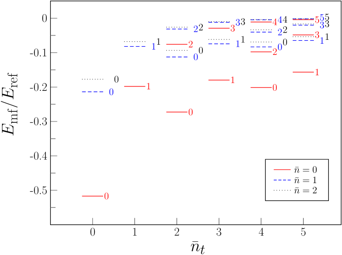
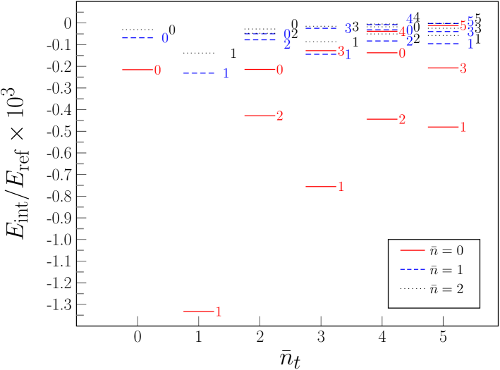
Figure 1: (Color online) Mean-field energy (33) and interaction energy (34), plotted as a function of $\bar{n}_{t}$. The number affixed to each bar denotes the value of $|\bar{m}|$.

The mean-field energy dominates the binding energy of a polaron in comparison with the interaction energy. The ground state is given by the impurity state $(\bar{n}=0,\bar{n}_{t}=0,\bar{m}=0)$, followed by the first and second excited states of $(\bar{n}=0,\bar{n}_{t}=2,\bar{m}=0)$ and $(\bar{n}=1,\bar{n}_{t}=0,\bar{m}=0)$, which can be accounted for by a larger overlap of the wave function of the BEC with those of $\bar{m}=0$ impurity states than $\bar{m}\neq 0$ (see the mean-field energy (33) with (25)). It should be noted that the interaction energy for $\bar{m}=0$ is equivalent to the second-order perturbation due to virtual boson excitations, because $f_{n,n_{t},m;u}=0$ for $m\neq 0$ (see Eq. (29) with $\left\langle\frac{1}{r^{2}}\right\rangle_{u}=\frac{m_{f}\omega_{ft}}{|\bar{m}|}$) and hence only $m=0$ states for boson excitations contribute to the summation in (34). This, in turn, leads to no drag effect $\eta=0$ for $\bar{m}=0$ via (31), as will be seen again later.

Looking into the dependence of the interaction energy on the quantum numbers $u=(\bar{n},\bar{n}_{t},\bar{m})$, we find that the states with $|\bar{m}|=1$ for $\bar{n}_{t}=1,3,5$ gain relatively larger interaction energies than others. This tendency can be understood from the fact that, in the summation over a given $m$ and $-m$ in (34), the denominator gets smaller for larger values of $|\bar{m}|$, while the overlap integral $\bar{C}_{n,n_{t},m;\bar{n},\bar{n}_{t},\bar{m}}$ in the numerator gets smaller even more rapidly. From the above observation, it turns out that the interaction between the impurity and bosons breaks the degeneracy of the single particle energy $E_{u}^{f}$ for a bare impurity state $u=(\bar{n},\bar{n}_{t},\bar{m})$ with respect to $\bar{m}$, and that the mean-field and interaction energies split for $|\bar{m}|\leq\bar{n}_{t}$, where $\bar{n}_{t}\geq 2$ (the reflection symmetry still keeps any $\bar{m}$ and $-\bar{m}$ states degenerate).

Here we should mention that experimental observations of motional coherence of trapped impurity atoms in the two lowest energy levels, in both the presence and the absence of the BEC background, has recently been achieved by motional Ramsey spectroscopy Scelle1 , which leads to the energy shift of the trapped impurity due to coupling with the BEC background, i.e., “phononic Lamb shift”, for a weakly coupled impurity-boson interaction Rentrop1 . In analyzing this experimental result, Bogoliubov phonons of the BEC in free space and impurities trapped only in a single dimension were used. In this analysis, the angular momentum is not relevant. However, such experimental techniques could be utilized also for observations of fine level splittings between different angular momenta obtained in the present study.

IV.2 Drag parameter $\eta$ and the number of excited bosons

The above observation about the $\bar{m}\neq 0$ states also reflects the drag parameter (31) and the number of excited bosons due to the interaction with the impurity, which is defined by

$$N_{\rm exc}=\sum_{s\neq 0}\langle b_{s}^{\dagger}b_{s}\rangle={\sum_{n,n_{t},m}}^{\prime}|f_{n,n_{t},m;u}|^{2}$$ (40)

with $f_{n,n_{t},m;u}$ given by (30).

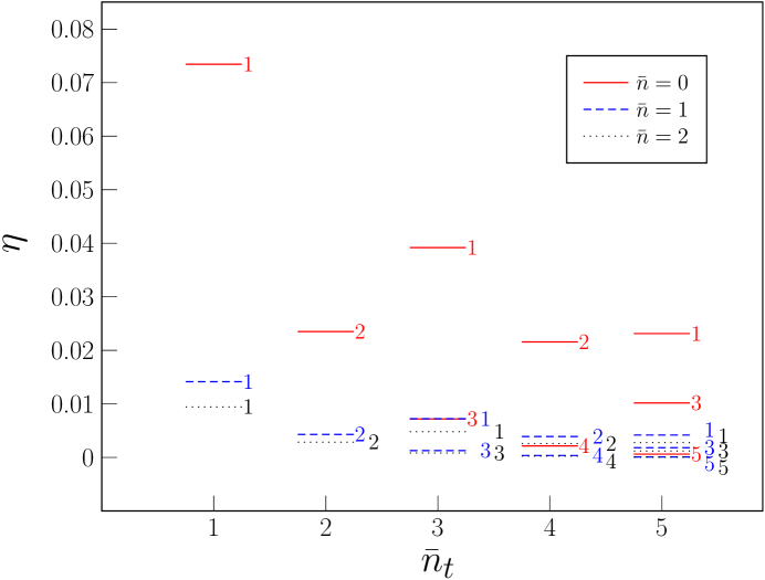
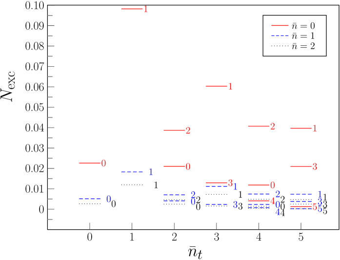
Figure 2: (Color online) Drag parameter (31) and the number of excited bosons (40), plotted as a function of $\bar{n}_{t}$. The number affixed to each bar denotes the value of $|\bar{m}|$.

As shown in Fig. 2, the drag parameter $\eta$ becomes nonzero for the $\bar{m}\neq 0$ states, which takes on an especially large value for the $|\bar{m}|=1$ states for a reason similar to the case of the interaction energy. Also, the distribution of $\eta$ has a pattern common to that of the number of excited bosons, except that the latter is nonzero even for the $\bar{m}=0$ states. This behavior is natural because $\eta$ is a fraction of the total angular momentum of a polaron carried by excited bosons.

The number of excited bosons also tells us if the present Bogoliubov-type approximation is valid. Figure 2 shows that $N_{\rm exc}$ is about $0.1$ at most. If $N_{\rm exc}$ is around unity, it obviously implies a breakdown of the present approximation, so that we need to restore the four-point residual interaction between the impurity and excited bosons, which is responsible for correlation effects such as quasibound states among the impurity and bosons.

IV.3 Extension to strong coupling regime and lighter bosons

Hitherto we have fixed the coupling strength $g$ to a constant that lies in a weak coupling regime. Now we take some typical values of the coupling strength to observe how the system transforms toward the strong coupling regime, and illustrate in Fig. 3 the coupling strength dependence of the binding energy of a polaron, which is defined by

$$E_{\rm bound}\equiv E_{\rm mf}+E_{\rm int},$$ (41)

and the number of excited bosons (40). The figure shows that the binding energy increases monotonically in magnitude and that there appears a bunch of excited states above the ground state $(\bar{n},\bar{n}_{t},\bar{m})=(0,0,0)$, which do not undergo level crossings with increasing coupling strength. Moreover, the number of excited bosons, being largest for the state of $(\bar{n},\bar{n}_{t},|\bar{m}|)=(0,1,1)$, increases above $0.5$ at $(a_{bf}k_{\rm ref})^{-1}=-2$, which implies the limitation of the present approximation where the residual boson-fermion interaction is assumed to be negligible, i.e., $b_{s^{\prime}}^{\dagger}b_{s}\ll 1$.

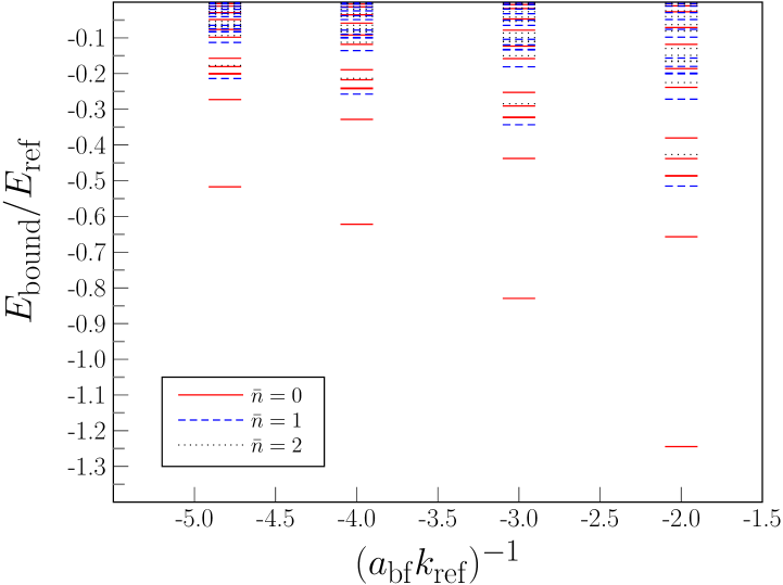
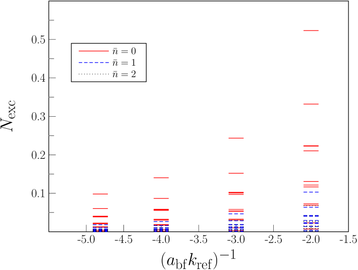
Figure 3: (Color online) The polaron’s binding energy (41) and the number of excited bosons (40) for $\bar{n}=0,1,2$, and $\bar{n}_{t}=0,1,2,3,4,5$, plotted as a function of the inverse scattering length $(a_{bf}k_{\rm ref})^{-1}=-4.813,-4,-3,-2$. Indication of the quantum numbers $(\bar{n}_{t},\bar{m})$ for each bar is omitted.

It is also interesting to see how our results are modified when bosons are significantly lighter than an impurity, since the LLP theory works better for relatively heavier impurities LLP1 ; Schweber1 . In the dimensionless expressions for the mean-field and interaction energies (see (53) and (54) in the Appendix), the dependence on the boson and fermion mass can be factored out except for rescaling factors of the boson’s coordinates in the wave functions, $z=R\zeta$ and $r=R_{t}\rho$, which propagates to the overlap integrals inherent in $\tilde{C}_{s,u}(R,R_{t})$ in (54). In the case of a heavy impurity and/or light bosons, the overlap of the wave functions of the condensed and excited bosons becomes larger at the origin in the integral, which leads to a possible enhancement of these energies.

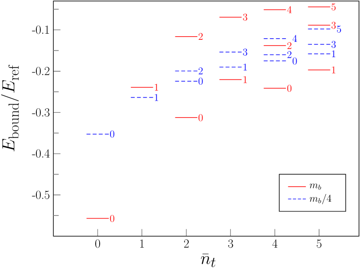
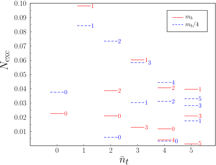
Figure 4: (Color online) The polaron’s binding energy (41) and the number of excited bosons (40) for the boson mass of $m_{b}$ and $m_{b}/4$, $(a_{bf}k_{\rm ref})^{-1}=-4.813$, $\bar{n}=0$, plotted as a function of $\bar{n}_{t}$. The number affixed to each bar denotes the value of $|\bar{m}|$.

In Fig. 4 we show the binding energy obtained by replacing the boson mass $m_{b}$ with $m_{b}/4$, which is about a half of $m_{f}$. We find from the figure that the virtual excitation of bosons is favored and that a larger binding energy is gained in comparison with the results obtained for the boson mass $m_{b}$ and the same coupling constant $1/a_{bf}k_{\rm ref}=-4.813$. It is interesting to observe that the number of excited bosons gets larger for higher angular momentum states, in contrast to the heavier boson case. This is because the overlap integrals associated with $\tilde{C}_{s,u}(R,R_{t})$ in (51) are enhanced for lighter bosons. These results imply that the salient features obtained in this study, such as the energy splitting and the drag effect for nonzero angular momentum states, become more prominent for $m_{b}\ll m_{f}$.

V Summary and Outlooks

We have investigated the properties of a single BEC polaron trapped in an axially symmetric harmonic potential in a weak to intermediate coupling regime, and for this purpose we have developed a formulation based on an LLP-type variational method LLP1 . We have obtained the mean-field energy (33) of ${\mathcal{O}}\left(g\right)$, whose magnitude is determined by the overlap of wave functions between the impurity and BEC states, and dominates the total binding energy of a polaron. We have also found that the interaction between the impurity and excited bosons breaks the level degeneracy with respect to the total angular momentum around the symmetric axis. Our result shows that the interaction energy (34) includes an overall factor of ${\mathcal{O}}\left(g^{2}\right)$ and also a non-perturbative effect through the coefficient $\eta$, the ratio of the angular momentum carried by excited bosons to the total angular momentum $\bar{m}$, but in the case of $\bar{m}=0$ the interaction energy reduces to the second-order perturbation theory involving virtual boson excitations. This situation is similar to the LLP description of spatially uniform electron-phonon systems, according to which a drag parameter $\eta$ is introduced for the total momentum of a polaron. Possible improvement beyond the present approximation to which we have simply taken a single eigenstate given by the harmonic potential for the impurity is that we can variationally determine the impurity state as well, especially for ${\bar{m}}=0$.

For elaborate comparison with experimental results in a weak to strong coupling regime, there remain several steps: When the $s$-wave scattering for boson-boson interactions is turned on, the excitation spectrum of the boson sector would be modified, e.g., in the Thomas-Fermi regime the energy dependence on the quantum numbers would be drastically changed Dalfovo1 ; Pitaevskii1 . For a microscopic description of such a semi-classical regime we need to solve, e.g., the Gross-Pitaevskii equation for the condensed and excited states, and obtain the effective low energy modes coupled to the impurity Japha1 . In the real experimental situations, impurity atoms themselves can form many-body systems and hence possible realizations of many-polaron systems if they are dilute enough for the quasiparticle picture to be valid. In such cases we need to take into account the particle statistics of impurities, e.g., Pauli blocking effect for fermionic impurities, in addition to finite temperature effects, and also effects of interaction among polarons LDB2 ; Casteels5 ; LDB3 ; NY1 ; Naidon1 , which may modify the polaron properties such as the spectral width and life time.

For strong coupling near the unitary limit of the boson-impurity interaction, or even for intermediate coupling, the present approximation seemingly breaks down. In these regimes we have to restore the four-point boson-impurity interaction, which has been discarded in the present Bogoliubov-type approximation, but is responsible for scattering processes between the impurity and excited bosons and, around the unitary limit, for quasi bound states between them Rath1 . For a smooth description of trapped systems from a weak to strong coupling regime, it might be convenient to build such few-body correlations (quasi bound states) among the impurity and bosons into the present LLP-type approximation Shchadilova2 .

Acknowledgments

E.N. is partially supported by Grants-in-Aid for Scientific Research through Grant No. 16K05349 provided by JSPS, and K.I. is partially supported by Grants-in-Aid for Scientific Research on Innovative Areas through Grant No. 24105008 provided by MEXT.

Appendix A Dimensionless variables for numerical calculations

We introduce the dimensionless variables, $\zeta\equiv\sqrt{m_{f}\omega_{f}}z$ and $\rho\equiv\sqrt{m_{f}\omega_{ft}}r$, and the normalized eigenfunctions as

$$\phi_{n,n_{t},m}(\zeta,\rho,\varphi) = \frac{1}{\sqrt{2\pi}}e^{im\varphi}\psi_{n}(\zeta)\psi_{n_{t},|m|}(\rho),$$ (42)

$$\int_{-\infty}^{\infty}{\rm d}\zeta\psi_{n}^{*}(\zeta)\psi_{n^{\prime}}(\zeta) = \delta_{n,n^{\prime}},\quad\int_{0}^{\infty}{\rm d}\rho\rho\psi_{n_{t},|m|}^{*}(\rho)\psi_{n_{t}^{\prime},|m|}(\rho)=\delta_{n_{t},n_{t}^{\prime}},$$ (43)

where

$$\psi_{n}(\zeta) := \sqrt{\frac{1}{2^{n}n!\sqrt{\pi}}}e^{-\frac{1}{2}\zeta^{2}}H_{n}\left(\zeta\right),$$ (44)

$$\psi_{n_{t},|m|}(\rho) := \sqrt{2\frac{\left(\frac{n_{t}-|m|}{2}\right)!}{\left(\frac{n_{t}+|m|}{2}\right)!}}\rho^{|m|}e^{-\frac{1}{2}\rho^{2}}L_{\frac{n_{t}-|m|}{2}}^{|m|}\left(\rho^{2}\right).$$ (45)

Relations to the normalized eigenfunctions with the original coordinates are given by

$$\Psi_{n}(z) = \left(m_{f}\omega_{f}\right)^{1/4}\psi_{n}(\sqrt{m_{f}\omega_{f}}z),$$ (46)

$$\Psi_{n_{t},m}(r) = \left(m_{f}\omega_{ft}\right)^{1/2}\psi_{n_{t},m}(\sqrt{m_{f}\omega_{ft}}r).$$ (47)

For numerical calculations, various quantities are given in terms of the corresponding dimensionless quantities:

$$\left\langle\frac{1}{r^{2}}\right\rangle_{\bar{n},\bar{n}_{t},\bar{m}} = m_{f}\omega_{ft}\int_{0}^{\infty}{\rm d}\rho\rho^{-1}|\psi_{\bar{n}_{t},\bar{m}}(\rho)|^{2}=\frac{m_{f}\omega_{ft}}{|\bar{m}|},$$ (48)

where $|\bar{m}|=\bar{n}_{t},\bar{n}_{t}-2,\bar{n}_{t}-4,\cdots,1\mbox{ or }0$,

$$\bar{C}_{n,n_{t},m;\bar{n},\bar{n}_{t},\bar{m}} \equiv \int_{\bf x}\Phi_{n,n_{t},m}({\bf x})\left|\phi^{f}_{\bar{n},\bar{n}_{t},\bar{m}}({\bf x})\right|^{2}=\sqrt{\omega_{b}m_{b}}\,\omega_{bt}m_{b}\,\tilde{C}_{n,n_{t},m;\bar{n},\bar{n}_{t},\bar{m}}\left(R,R_{t}\right),$$ (49)

where $R=\sqrt{\frac{\omega_{b}m_{b}}{\omega_{f}m_{f}}}$, $R_{t}=\sqrt{\frac{\omega_{bt}m_{b}}{\omega_{ft}m_{f}}}$, and

$$\tilde{C}_{n,n_{t},m;\bar{n},\bar{n}_{t},\bar{m}}\left(R,R_{t}\right) \equiv \frac{1}{2\pi}\int_{-\infty}^{\infty}{\rm d}\zeta\psi_{0}^{*}(R\zeta)\psi_{n}(R\zeta)\left|\psi_{\bar{n}}(\zeta)\right|^{2}$$ (50)

$$\times\int_{0}^{\infty}{\rm d}\rho\rho\psi_{0,0}^{*}(R_{t}\rho)\psi_{n_{t},m}(R_{t}\rho)\left|\psi_{\bar{n}_{t},\bar{m}}(\rho)\right|^{2}.$$

A.1 Probability amplitude

In the formula for the number of excited bosons (40), the probability amplitude squared can be rewritten in terms of the dimensionless variables as

$$|f_{n,n_{t},m;u}|^{2} = N_{0}G^{2}\frac{|\tilde{C}_{n,n_{t},m;\bar{n},\bar{n}_{t},\bar{m}}\left(R,R_{t}\right)|^{2}}{\left[\frac{\omega_{b}}{\omega_{ft}}\left(n+\frac{1}{2}\right)+\frac{\omega_{bt}}{\omega_{ft}}\left(n_{t}+1\right)+\frac{m^{2}-2\left(1-\eta\right)\bar{m}m}{2|\bar{m}|}\right]^{2}},$$ (51)

$$G \equiv \left(2\pi a_{bf}\sqrt{\omega_{b}m_{b}}\right)\left(\frac{m_{f}}{m_{b}}+1\right)R_{t}^{2}.$$ (52)

The above expression can also be used in the self-consistent Eq. (31) for $\eta$. Note that we cannot expand the right hand side of the self-consistent equation to the linear-order in $\bar{m}$, unlike the drag parameter for the polaron’s total momentum in the LLP theory for uniform systems.

A.2 Mean-field and interaction energies

The mean-field and interaction energies for the state of $u=(\bar{n},\bar{n}_{t},\bar{m})$ become

$$\frac{E_{{\rm mf},u}}{\omega_{ft}} = N_{0}G\,\tilde{C}_{0,0,0;\bar{n},\bar{n}_{t},\bar{m}}\left(R,R_{t}\right),$$ (53)

$$\frac{E_{{\rm int},u}}{\omega_{ft}} = -\frac{|\bar{m}|\eta^{2}}{2}-N_{0}G^{2}\sum_{n,n_{t}(\neq 0),m}\frac{|\tilde{C}_{n,n_{t},m;\bar{n},\bar{n}_{t},\bar{m}}\left(R,R_{t}\right)|^{2}}{\frac{\omega_{b}}{\omega_{ft}}\left(n+\frac{1}{2}\right)+\frac{\omega_{bt}}{\omega_{ft}}\left(n_{t}+1\right)+\frac{m^{2}-2\left(1-\eta\right)\bar{m}m}{2|\bar{m}|}}.$$ (54)

References

• (1) See, for instance, Gerald D.Β Mahan, Many-Particle Physics (Springer, 1990).
• (2) For instance, see, A.Β S.Β Alexandrov, J.Β T.Β Devreese, Advances in Polaron Physics, Springer Series in Solid-State Sciences Vol. 159, (Springer, 2009).
• (3) L.Β D.Β Landau, Phys.Β Z.Β Sowjetunion 3, 664 (1933); L.Β Landau and S.Β Pekar, J.Β Exptl.Β Theor.Β Phys. 18, 419 (1948); S.Β Pekar, J.Β Exptl.Β Theor.Β Phys. 19, 796 (1949).
• (4) H.Β FrΓΆhlich, Theory of Dielectrics, (Clarendon Press, Oxford, 1949); H.Β FrΓΆhlich, H.Β Pelzer, and S.Β Zienau, Phil.Β Mag. 41, 221 (1950); H.Β FrΓΆhlich, Adv.Β Phys. 3, 325 (1954).
• (5) T.Β D.Β Lee, F.Β E.Β Low, and D.Β Pines, Phys.Β Rev.Β 90, No.2, 297-302 (1953).
• (6) F.Β M.Β Cucchietti and E.Β Timmermans, Phys.Β Rev.Β Lett.Β 96, 210401 (2006).
• (7) K.Β Sacha and E.Β Timmermans, Phys.Β Rev.Β A 73, 063604 (2006).
• (8) J.Β Tempere, W.Β Casteels, M.Β K.Β Oberthaler, S.Β Knoop, E.Β Timmermans, and J.Β T.Β Devreese, Phys.Β Rev.Β B 80, 184504 (2009).
• (9) W.Β Casteels, T.Β VanΒ Cauteren, J.Β Tempere, and J.Β T.Β Devreese, Laser Physics 21, 8, pp 1480-1485 (2011).
• (10) S.Β P. Rath and R.Β Schmidt, Phys.Β Rev.Β A, 88, 053632 (2013)
• (11) A.Β Shashi, F.Β Grusdt, D.Β A.Β Abanin, and E.Β Demler, Phys.Β Rev.Β A, 89, 053617 (2014).
• (12) Jesper Levinsen, Meera M. Parish, and GeorgΒ M. Bruun, Phys.Β Rev.Β Lett.Β 115, 125302 (2015).
• (13) A.Β S.Β Dehkharghani, A.Β G.Β Volosniev, and N.Β T.Β Zinner, Phys.Β Rev.Β A 92, 031601(R) (2015).
• (14) L.Β A.Β PeΓ±aΒ Ardila and S.Β Giorgini, Phys.Β Rev.Β A 92, 033612 (2015).
• (15) T.Β Yin, D.Β Cocks and W.Β Hofstetter, Phys.Β Rev.Β A, 92, 063635 (2015).
• (16) R.Β S.Β Christensen, J.Β Levinsen, and G.Β M.Β Bruun, Phys.Β Rev.Β Lett. 115, 160401 (2015)
• (17) J.Β Vlietinck, W.Β Casteels, K.Β VanΒ Houcke, J.Β Tempere, J.Β Ryckebusch, and J.Β T.Β Devreese, New J.Β Phys.Β 17,033023 (2015).
• (18) F.Β Grusdt, Y.Β E.Β Shchadilova, A.Β N.Β Rubtsov, and E.Β Demler, Sci.Β Rep.Β 5, 12124 (2015).
• (19) F.Β Grusdt and M.Β Fleischhauer, Phys.Β Rev.Β Lett.Β 116, 053602 (2016).
• (20) Y.Β E.Β Shchadilova, F.Β Grusdt, A.Β N.Β Rubtsov, and E.Β Demler, Phys.Β Rev.Β A93, 043606 (2016)
• (21) F.Β Chevy, Phys.Β Rev.Β AΒ 74, 063628 (2006).
• (22) André Schirotzek, Cheng-HsunΒ Wu, ArielΒ Sommer, and MartinΒ W.Β Zwierlein, Phys.Β Rev.Β Lett.Β 102, 230402 (2009).
• (23) R.Β Schmidt and T.Β Enss, Phys.Β Rev.Β A 83, 063620 (2011).
• (24) C.Β Kohstall, M.Β Zaccanti, M.Β Jag, A.Β Trenkwalder, P.Β Massignan, G.Β M.Β Bruun, F.Β Schreck, and R.Β Grimm, NatureΒ 485, 615-618 (2012).
• (25) M.Β Koschorreck, D.Β Pertot, E.Β Vogt, B.Β FrΓΆhlich, M.Β Feld, and M.Β KΓΆhl, Nature 485, 619 (2012).
• (26) J.Β Vlietinck, J.Β Ryckebusch, and K.Β VanΒ Houcke, Phys.Β Rev.Β B 87, 115133 (2013).
• (27) Pietro Massignan, Matteo Zaccanti, and GeorgΒ M. Bruun, Reports on Progress in Physics, Volume 77, Number 3, (2014).
• (28) W.Β Yi and X.Β Cui Phys.Β Rev.Β A 92, 013620 (2015).
• (29) M.Β Bruderer, AlexanderΒ Klein, StephenΒ R.Β Clark, and DieterΒ Jaksch, Phys.Β Rev.Β A, 76(R):011605 (2007); NewΒ J.Β Phys.Β 10, 033015 (2008).
• (30) J.Β Catani, G.Β Lamporesi, D.Β Naik, M.Β Gring, M.Β Inguscio, F.Β Minardi, A.Β Kantian, and T.Β Giamarchi, Phys.Β Rev.Β A 85, 023623 (2012).
• (31) R.Β Scelle, T.Β Rentrop, A.Β Trautmann, T.Β Schuster, and M.Β K.Β Oberthaler, Phys.Β Rev.Β Lett.Β 111, 070401 (2013).
• (32) M.Β Hohmann, F.Β Kindermann, B.Β GΓ€nger, T.Β Lausch, D.Β Mayer, F.Β Schmidt and A.Β Widera, EPJ Quantum Technology 2:23, (2015)
• (33) Nils B.Β JΓΈrgensen, Lars Wacker, Kristoffer T.Β Skalmstang, Meera M.Β Parish, Jesper Levinsen, Rasmus S.Β Christensen, Georg M.Β Bruun, Jan J.Β Arlt, Phys.Β Rev.Β Lett.Β 117, 055302 (2016).
• (34) Ming-Guang Hu, Michael J. Van de Graaff, Dhruv Kedar, John P.Β Corson, EricΒ A.Β Cornell, and Deborah S.Β Jin, Phys.Β Rev.Β Lett.Β 117, 055301 (2016).
• (35) See, for instance, C.Β J.Β Pethick and H.Β Smith, Bose-Einstein Condensation in Dilute Gases (Cambridge University Press, Cambridge, 2008).
• (36) Franco Dalfovo, Stefano Giorgini, Lev P. Pitaevskii, and Sandro Stringari, Rev.Β Mod.Β Phys.Β 71, 463 (1999).
• (37) See, for instance, L.Β Pitaevskii and S.Β Stringari, Bose-Einstein Condensation (Oxford, New York, 2003).
• (38) ElizabethΒ A.Β Donley, NeilΒ R.Β Claussen, SimonΒ L.Β Cornish, JacobΒ L.Β Roberts, EricΒ A.Β Cornell, and CarlΒ E.Β Wieman, Nature 412, 295-299 (2001).
• (39) ThomasΒ Volz, StephanΒ DΓΌrr, SebastianΒ Ernst, AndreasΒ Marte, and GerhardΒ Rempe, Phys.Β Rev.Β A 68, 010702(R) (2003).
• (40) ErichΒ J.Β Mueller and GordonΒ Baym, Phys.Β Rev.Β A 62, 053605 (2000); arXiv:cond-mat/9908133.
• (41) Quantum mechanics in one- and two-electron atoms, HansΒ A.Β Bethe and EdwinΒ E.Β Salpeter, (Plenum Publishing Corporation, New York, 1977).
• (42) D.Β R.Β Inglis, Phys.Β Rev.Β 96, 1059 (1954) ; Β 96, 701 (1955).
• (43) D.Β J.Β Thouless and J.Β G.Β Valatin, Nucl.Β Phys.Β 31, 211-230 (1962).
• (44) Richard Schmidt and Mikhail Lemeshko, Phys.Β Rev.Β X 6, 011012 (2016).
• (45) RichardΒ Schmidt and MikhailΒ Lemeshko, Phys.Β Rev.Β Lett.Β 114, 203001 (2015).
• (46) Nicolas Spethmann, Farina Kindermann, Shincy John, Claudia Weber, Dieter Meschede, and Artur Widera, Phys.Β Rev.Β Lett.Β 109, 235301 (2012).
• (47) T.Β Rentrop, A.Β Trautmann, F.Β A.Β Olivares, F.Β Jendrzejewski, A.Β Komnik, and M.Β K.Β Oberthaler, Phys.Β Rev.Β X 6, 041041 (2016).
• (48) S.Β S.Β Schweber, An Introduction to Relativistic Quantum Field Theory, (Dover Publications, New York, 2005).
• (49) Y.Β Japha and Y.Β B.Β Band, Phys.Β  Rev.Β  A 84, 033630 (2011).
• (50) W.Β Casteels, J.Β Tempere, and J.Β T.Β Devreese, Phys.Β Rev.Β A 84, 063612 (2011).
• (51) W.Β Casteels, J.Β Tempere, and J.Β T.Β Devreese, Phys.Β Rev.Β A 88, 013613 (2013).
• (52) W.Β Casteels, J.Β Tempere and J.Β T.Β Devreese, Eur.Β Phys.Β J.Β SpecialΒ Topics 217, 163 (2013).
• (53) E.Β Nakano and H.Β Yabu, Phys.Β Rev.Β B 93, 205144 (2016).
• (54) Two impurities in a Bose-Einstein condensate, P.Β Naidon, arXiv: 1607.04507.
• (55) Yulia E.Β Shchadilova, Richard Schmidt, Fabian Grusdt, and Eugene Demler, Phys.Β Rev.Β  Lett. Β 117, 113002 (2016).