Liquid-Liquid Critical Point in 3D Many-Body Water Model

Abstract

Many-body interactions can play a relevant role in water properties. Here we study by Monte Carlo simulations a coarse-grained model for bulk water that includes many-body interactions associated to water cooperativity. The model is efficient and allows us to equilibrate water at extreme low temperatures in a wide range of pressures. We find the line of temperatures of maximum density at constant pressure and, at low temperature and high pressure, a phase transition between high-density liquid and low-density liquid phases. The liquid-liquid phase transition ends in a critical point. In the supercritical liquid region we find for each thermodynamic response function a locus of weak maxima at high temperature and a locus of strong maxima at low temperature, with both loci converging at the liquid-liquid critical point where they diverge. Comparing our results with previous works for the phase diagram of a many-body water monolayer, we observe that the weak maxima of the specific heat are less evident in bulk and appear only at negative pressures, while we find those of compressibility and thermal expansion coefficient also at positive pressures in bulk. However, the strong maxima of compressibility and thermal expansion coefficient are very sharp for the bulk case. Our results clarify fundamental properties of bulk water, possibly difficult to detect with atomistic models not accounting for many-body interactions.

I Introduction

Water models are of fundamental importance in many fields of physics, chemistry, biology and engineering. For example, it is now commonly accepted that water plays a key role in protein folding Levy and Onuchic (2004); Franzese et al. (2011); Bianco et al. (2012); Bianco and Franzese (2015); Sirovetz et al. (2015); Mallamace et al. (2016) and protein dynamics Johnson et al. (2008); Ngai et al. (2008); Mazza and et al. (2011); Schirò and et al. (2015); Fogarty and Laage (2014); Mallamace et al. (2015). Computer simulations are an important tool to study such phenomena. Nevertheless, the computational cost for full-atom simulations of large-scale biological systems with explicit water for experimentally-relevant time-scales is often prohibitive. Therefore, it is necessary to explore alternative approaches that could allow us to access mesoscopic scales and time-scales of the order of seconds. A possible solution is to develop coarse-grain models of water that could greatly reduce the simulation cost for the solvent preserving its main physical properties.

Despite the importance of water in many aspects of life, there are still open questions concerning its complex nature. Water exhibits more than 60 anomalies Chaplin (2006), like the existence of a density maximum in the liquid phase at ambient pressure and temperature $T\sim 4^{\circ}$C or the anomalous increase of the specific heat $C_{P}$, isothermal compressibility $K_{T}$, and absolute value of the thermal expansivity $\alpha_{P}$ upon cooling liquid water toward the melting line and below it, in the supercooled liquid state Debenedetti (1996). A common understanding is that all these peculiar properties of water are related to its hydrogen bonds (HBs) forming a network that orders following tetrahedral patterns at low $T$ Errington and Debenedetti (2001). A large number of classical atomistic water models have been proposed in the last decades with some performing better than others Vega et al. (2009). Nevertheless, there is still no atomistic model able to fit all the water properties Vega et al. (2009). One possible reason for it is that pair-additive potentials do not capture the effective many-body interactions due to quantum effects and polarizability Barnes and et al. (1979); Cruzan and et al. (1996); Perez and et al. (2014); Guevara-Vela and et al. (2016). Consistent with this view, the effect of these many-body interactions are stronger where the water anomalies are more evident Agapov and et al. (2015).

The origin of anomalous properties of water has been largely debated since the 80’s Kanno and Angell (1979); Angell et al. (1982); Poole et al. (1994); Tanaka (1996); Mishima and Stanley (1998); Soper and Ricci (2000); Xu et al. (2005); Liu et al. (2007); Stokely et al. (2010); Abascal and Vega (2010); Bertrand and Anisimov (2011); Holten et al. (2013); Pallares et al. (2014); Bianco and Franzese (2014); Soper (2014); Nilsson and Pettersson (2015); Sciortino et al. (2011); Liu et al. (2012); Palmer et al. (2013); Poole et al. (2013); Palmer et al. (2014); Smallenburg and Sciortino (2015) and a series of thermodynamic scenarios have been proposed Speedy (1982); Sastry et al. (1996); Poole et al. (1992); Angell (2008). In particular, Poole et al., based on molecular dynamic simulations, proposed a liquid-liquid second critical point (LLCP) in the supercooled region Poole et al. (1992). According to this scenario, the LLCP is located at the end of a first order phase transition separating two liquid metastable phases of water with different density, structure and energy Liu et al. (2012); Bianco and Franzese (2014); Palmer et al. (2014). Extrapolations from experimental data Fuentevilla and Anisimov (2006), based on the hypothesis of such a critical point, show that the maxima in response functions should be much stronger and at lower temperature than those predicted by the classical model used in Ref. Poole et al. (1992). However, equilibrate classical models at very low $T$ is extremely computationally demanding, making difficult to settle the disagreement between the simulations and the extrapolated experimental data.

We propose a coarse grained (CG) bulk water model that includes many-body interactions in a computationally effective way. Our results extend those for a previous model of a many-body water monolayer, able to reproduces the main features of water in a very efficient way and at those extreme conditions that are not easily reachable by atomistic simulations Franzese et al. (2003); Franzese and Stanley (2002, 2007a, 2007b); de los Santos and Franzese (2011); Bianco and Franzese (2014). Here we show that the bulk model exhibits a liquid-liquid phase transition (LLPT) in the supercooled region, as the monolayer. We find a relevant difference between the results for the response functions in the the bulk model and those in the monolayer. In both cases we observe a line of weak maxima and a line of strong maxima for the response functions in the pressure-temperature phase diagram, however the $C_{P}$ weak maxima in bulk water are observable only at negative pressure, at variance with the monolayer case.

The paper is organized as follows. In Section II we define the coarse-grain model for bulk water with effective many-body interactions. In Section III we describe the simulation method. In Section IV we present and discuss our results. In Section V we give our conclusions. In Appendix A we present further details of the phase diagram and in Appendix B we explain the details of the equilibration and the error calculations.

II The Many-Body Water Model

We consider a system of a constant number of molecules $N$, pressure $P$ and temperature $T$ in a variable volume $V$. We partition the total volume $V$ into a regular cubic lattice of ${\cal N}$ cells, $i\in[1,...,{\cal N}]$, each with volume $v_{i}\equiv V/{\cal N}$. For sake of simplicity we set ${\cal N}=N$ and consider the case of a homogeneous fluid, in such a way that each cell is occupied by one water molecule. Next we introduce a discretized density field $n_{i}\equiv\theta(2-v_{i}/v_{0})$, where the Heaviside step function $\theta(x)$ is 0 or 1 depending if $x<0$ or $\geq 0$, corresponding to gas-like or liquid-like local density, respectively, and $v_{0}\equiv 4/3\pi(r_{0}/2)^{3}$ is the van der Waals volume of a water molecules, with $r_{0}\equiv 2.9$ Å.

The Hamiltonian of the system is by definition the sum of three terms

$$\mathscr{H}\equiv\mathscr{H}_{\rm vdW}+\mathscr{H}_{\rm HB}+\mathscr{H}_{\rm coop},$$ (1)

corresponding to the van der Waals isotropic interaction, the directional and the cooperative contribution to the HB interaction, respectively. A detailed description and motivation for each term can be found in Ref.s Franzese and Stanley (2007a); de los Santos and Franzese (2011); Bianco and Franzese (2014).

The van der Waals Term is given by the sum over the contributions of all pairs of molecules $i$ and $j$,

$$\mathscr{H}_{\rm vdW}\equiv\sum_{<i,j>}U(r_{ij}),$$ (2)

where $U(r)$ is a Lennard-Jones potential with a hard-core (van der Waals) diameter $r_{0}$, i.e.

$$U(r)\equiv\left\{\begin{array}[]{ll}\infty&\textup{if}\ r\leq r_{0}\\ \epsilon\left[\left(\frac{r_{0}}{r}\right)^{12}-\left(\frac{r_{0}}{r}\right)^{6}\right]&\textup{if}\ r_{0}>r>r_{c}\\ 0&\textup{if}\ r_{c}<r.\end{array}\right.$$ (3)

We truncate the interaction at a distance $r_{c}\equiv 6r_{0}$.

The second terms in Eq. (1) is defined as

$$\mathscr{H}_{\rm HB}\equiv-JN_{\rm HB}\equiv-J\sum_{<ij>}n_{i}n_{j}\delta_{\sigma_{ij}\sigma_{ji}}$$ (4)

where $N_{\rm HB}$ is the total number of HB in the system. A water molecule $i$ can form up to four HBs with molecules $j$ at a distance such that $n_{i}n_{j}=1$, i.e. $v_{i}\leq 2v_{0}$ implying a water-water distance $r_{i,j}\leq 2^{1/3}r_{0}\simeq 3.7$ Å. Furthermore, to form a HB the relative orientation of the two water molecules must be such that the angle between the OH of a molecules and the O-O direction does not exceed $\pm 30^{o}$. Hence, only 1/6 of the entire range of values $[0,360^{o}]$ for this angle is associated to a bonding state. We account for this constrain introducing a bonding variable $\sigma_{ij}\in[1,q]$ of molecule $i$ with each of the six nearest molecules $j$ and setting $q=6$ to account correctly for $i)$ the contribution to the HB energy via the $\delta_{\sigma_{ij}\sigma_{ji}}\equiv 1$ if $\sigma_{ij}=\sigma_{ji}$, 0 otherwise, and $ii)$ the entropy variation due to the HB formation and breaking. We set $J/4\epsilon=0.5$, consistent with the proportion between the van der Waals interaction and the directional (covalent) part of the HB interaction.

The last term in the Hamiltonian accounts for the cooperativity of the HBs and is an effective many-body interaction between HBs due the O–O–O correlation that locally leads the molecules toward an ordered (tetrahedral) configuration

$$\mathscr{H}_{\rm coop}\equiv-J_{\sigma}N_{\rm coop}\equiv-J_{\sigma}\sum_{i}n_{i}\sum_{<kl>_{i}}\delta_{\sigma_{ik}\sigma_{il}},$$ (5)

where the sum is over the six bonding indices of the molecules $i$ with the molecules $k$ and $l$, both near $i$. By setting $J_{\sigma}/4\epsilon=0.03$, with $J_{\sigma}\ll J$, we guarantee that this term is relevant only at those temperatures below which the molecule $i$ has already formed (non-tetrahedral) HBs with the molecules $k$ and $l$, implying an effective many-body interaction of molecule $i$ with the four bounded molecules in its hydration shell.

A consequence of the formation of a network of tetrahedral HBs is the increase of proper volume associated to each molecule. The model takes this effect into account on average by adding a small increase of volume $v_{\rm HB}=0.5v_{0}$ per bond, consistent with the average volume increase between high-$\rho$ ices VI and VIII and low-$\rho$ (tetrahedral) ice Ih. Therefore, the total volume of the system with $N_{\rm HB}$ HBs is

$$V\equiv Nv_{0}+N_{\rm HB}v_{\rm HB}.$$ (6)

The tetrahedral local rearrangement does not change the average water-water distance, therefore the distance $r$ in Eq.(3) is not affected by the change in Eq.(6).

The enthalpy $H$ of the model is therefore

$$H\equiv\sum_{<i,j>}U(r_{ij})+JN_{\rm HB}+J_{\sigma}N_{\rm coop}+PV$$ (7)

and the volume contribution to the entropy is

$$S_{V}\equiv-k_{B}\ln(V/v_{0}).$$ (8)

The model presented here by definition does not include crystal phases, i.e. at any $T$ and $P$ our course grain water can be equilibrated in its fluid state after a large enough equilibration time. Furthermore in our coarse graining we neglect water translational diffusion, focusing only on the local rotational dynamics of the HBs. Formulation of the model that include translation diffusion and crystal polymorphism can be found in Ref. de los Santos and Franzese (2011) and Ref. Vilanova and Franzese (2011), respectively, for the monolayer case. Analogous formulations can be introduced also for the bulk model. It’s worth noting, however, that the present definition includes structural and densities heterogeneities associated to the HB network dynamics.

III Simulation method

We perform Monte Carlo (MC) simulations at constant $N=8000$, constant $P$ and constant $T$ in a cubic (variable) volume $V$ with periodic boundary conditions along two axis . We update the HB network with the Wolff Monte Carlo (MC) cluster algorithm adapted to the present model, as explained in Ref. Mazza et al. (2009).

We calculate the equation of state along isobars in the range of $Pv_{0}/(4\epsilon)\in[-0.5,0.95]$ separated by intervals of $\Delta P\leq 0.05(4\epsilon)/v_{0}$. The range of temperatures is $Tk_{B}/(4\epsilon)\in[0.02,1.0]$ with $\Delta T\geq 0.01(4\epsilon)/k_{B}$ if $Tk_{B}/(4\epsilon)\in(0.1,1.0]$, and $\Delta T\geq 0.001(4\epsilon)/k_{B}$, if $Tk_{B}/(4\epsilon)\in[0.02,0.1]$. We calculate each isobar by sequential annealing starting at $T=7(4\epsilon)/k_{B}$ and letting the system equilibrate, as explained in details in Appendix A. For each state point we average over $10^{6}$ MC steps after equilibration, with a number of independent configurations between $10^{2}$ – $10^{3}$ depending on the state point.

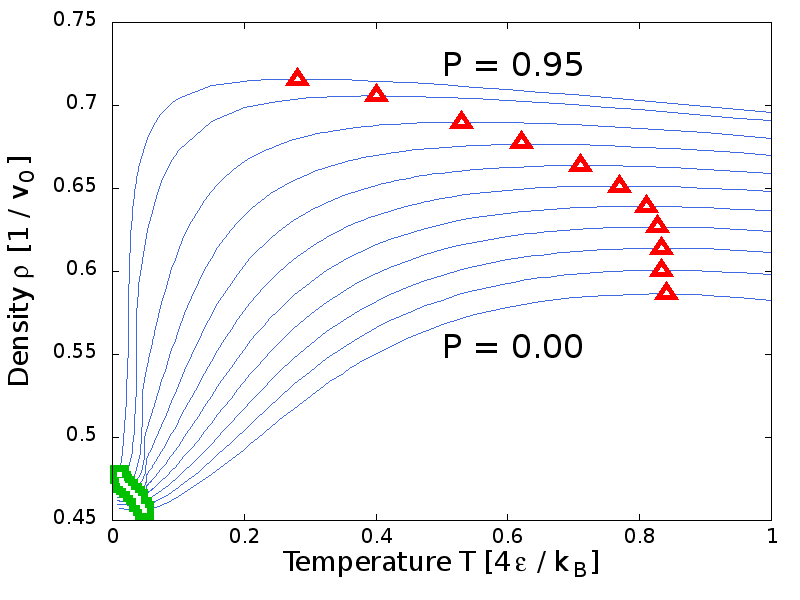
Figure 1: Density along isobars for (from bottom to top) $Pv_{0}/(4\epsilon)=0.00$, 0.10, 0.20, 0.30, 0.40, 0.50, 0.60, 0.70, 0.80, 0.90, 0.95. At each $P$ we find a temperature of maximum density, TMD (red triangles) and a temperature of minimum density, TminD (green squares). For sake of clarity we show the interpolated equation of state and do not show the calculated state points.

IV Results and discussion

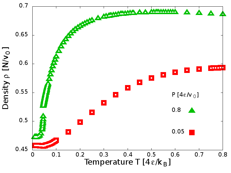
a) b)

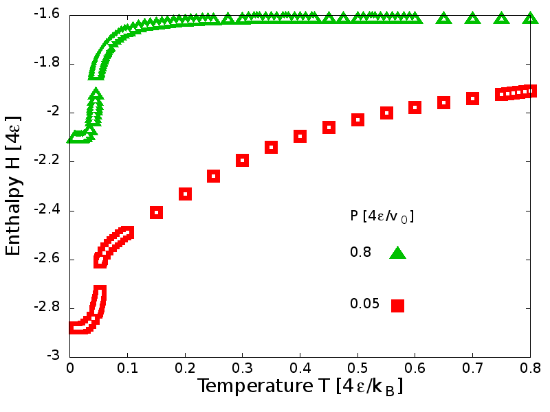
Figure 2: a) Isobaric variation of density and b) enthalpy as a function of temperature for high pressure ($Pv_{0}/(4\epsilon)=0.80$, green triangles) and low pressure ($Pv_{0}/(4\epsilon)=0.05$, red squares).

At temperatures below the gas-liquid phase transition (Appendix A), we find along isobars a temperature of maximum density (TMD) (Fig. 1) as in water. By further decreasing $T$, we observe a sharp decrease of the isobaric density $\rho\equiv N/V$ and a temperature of minimum density TminD (Fig. 1). This behavior is consistent with the LLPT between a high density liquid (HDL) and a low density liquid (LDL) as postulated for supercooled liquid water Poole et al. (1992). However, a similar behavior, but without any discontinuity, is predicted also by the “singularity free” scenario Stanley and Teixeira (1980); Sastry et al. (1996); Stokely et al. (2010). We therefore analyze the enthalpy behavior in detail.

We find that $H$ follows the density but with sharper changes at any $P$ (Fig. 2). At high $P$ both density and enthalpy display a seemingly discontinuous change, while for low $P$ the variation in density becomes much smother than the enthalpy change.

We understand the behavior of $\rho$ as a consequence of its dependence on $N_{\rm HB}$ from Eq.(6). A direct calculation shows that by decreasing $T$ the model displays a rapid increase of $N_{\rm HB}$ at high $P$, while the increase is progressive at low $P$ (Fig. 3a). In particular, we find that $N_{\rm HB}$ saturates at low $T$ to two HBs per molecule, corresponding to the case where every water molecule is involved in four HBs. At high $T$ the number $N_{\rm HB}/N$ is $\simeq 1/2$ at high $P$ and is $\simeq 0.7$ at low $P$, with each molecule forming on average one HB or less than two, respectively.

Nevertheless, the changes of $N_{\rm HB}$ are never discontinuous as in the enthalpy, clearly showing that the contribution to $H$ coming from the other terms in Eq.(7) are relevant. The explicit calculation of these terms shows that the dominant contribution comes from the behavior of $N_{\rm coop}$ (Fig. 3b). We find that $N_{\rm coop}$ has a sharp, but continuous, increase at any $P$ within the range investigated. Furthermore, at variance with what observed for $N_{\rm HB}$, the temperature of the largest increase of $N_{\rm coop}$ is almost independent on $P$. This temperature coincides with the largest variation of $H$ at any $P$ and with the large change of $\rho$ at high $P$.

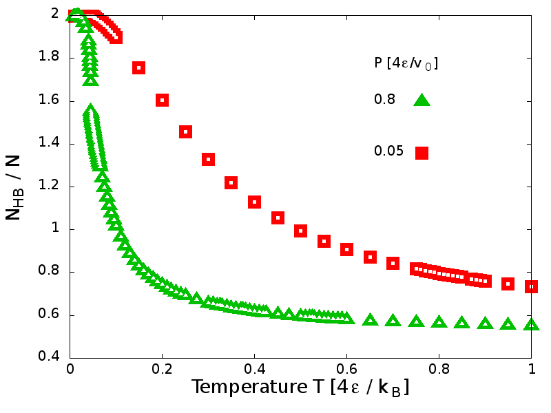
a) b)

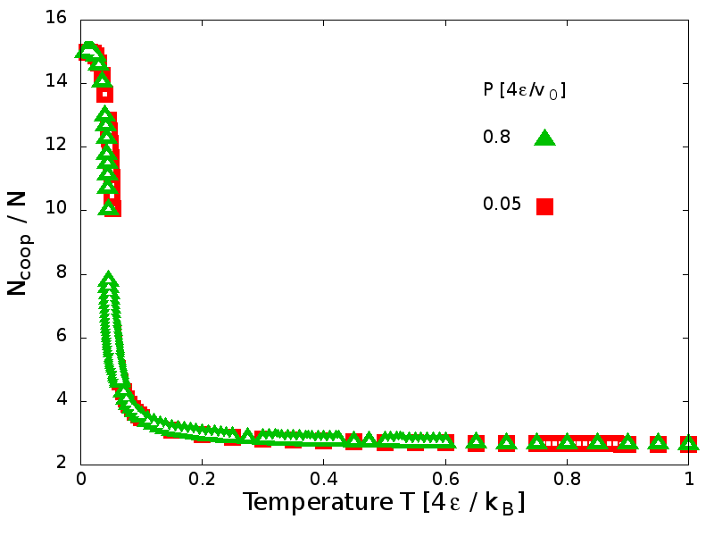
Figure 3: a) Isobaric variation of the number of HB per molecule $N_{\rm HB}/N$ and b) the number of cooperative bonds per molecule $N_{\rm coop}/N$. While $N_{\rm HB}$ strongly depend on $P$, $N_{\rm coop}$ is almost $P$-independent.

Therefore, the largest variation of $H$ is associated with the cooperative contribution that, in turns, is a consequence of a large structural rearrangement of the HBs toward a more tetrahedral configuration. However, at low $P$ this reorganization of the HBs occurs when the number $N_{\rm HB}$ of HBs is almost saturated, implying only a minor change in $\rho$. On the other hand, at high $P$ the restructuring of the HBs occurs at the same time as the formation of a large amount of them, up to saturation. Therefore, the effect on the density is large and collective, as expected at a critical phase transition.

A further way to clarify if the observed thermodynamic behavior is consistent with the occurrence of a LLPT ending in a critical point is to calculate the response functions $C_{P}$, $K_{T}$ and $\alpha_{P}$ and to study if they diverge at the hypothesized LLCP. At equilibrium all these quantities correspond to thermodynamic fluctuations. Therefore, we calculate the specific heat along isobars both by numerical derivative of $H$, $C_{P}\equiv(\partial\langle H\rangle/\partial T)_{P}$, and by the fluctuation-dissipation theorem $C_{P}=\langle H^{2}\rangle/k_{B}T^{2}$. In this way we reach a better estimate of $C_{P}$ and at the same time, by verifying the validity of fluctuation-dissipation theorem, we guarantee that the system is equilibrated (Appendix B).

We find strong maxima in $C_{P}$ at any $P$ and low $T$. For $Pv_{0}/(4\epsilon)\leq 0.85$ the maxima occur all at the same $T$ and increase as the pressure increases with an apparent divergence of $C_{P}$ at $Pv_{0}/(4\epsilon)=0.85$ (inset Fig. 4a). However, for $Pv_{0}/(4\epsilon)>0.85$ the maxima decrease in intensity and moves toward lower $T$ (Fig. 4a). This behavior is consistent with a LLCP occurring at $Pv_{0}/(4\epsilon)\simeq 0.85$ at the end of a first-order phase transition occurring at higher $P$ along a line with a negative slope in the $P$-$T$ thermodynamic plane, as expected in the LLCP scenario Poole et al. (1992).

By increasing the resolution at intermediate $T$ and exploring the metastable region of stretched water at $P<0$, we find weak maxima in $C_{P}$ at $T$ below the liquid-to-gas spinodal line (Fig. 4b). For increasing $P<0$ we find that the weak maxima occur at lower $T$ and progressively merge into the strong maxima.

The origin of these maxima was studied by Mazza et al. Mazza and et al. (2011) in the monolayer case. At any $P$ the weak maximum at high temperature is produced by the energy fluctuations during the formation of new HBs, while the strong maxima at low temperature is produced by the effect of the cooperative reordering of the HB network. This interpretation agrees with our results for the evolution along isobars of $N_{\rm HB}$ and $N_{\rm coop}$ (Fig. 3). However the weak $C_{P}$ maxima for the monolayer were observed also at $P>0$ and were slowly increasing in intensity for increasing $P$ before merging into the strong maxima Bianco and Franzese (2014), at variance with what we observe now for the bulk system.

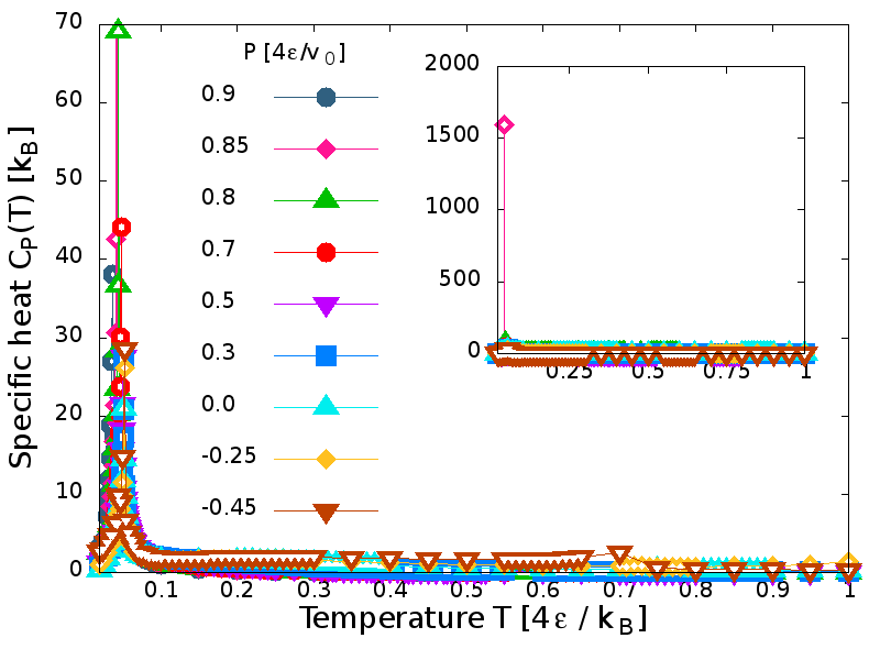
a) b)

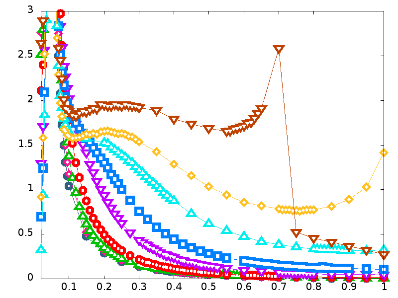
Figure 4: Isobaric specific heat $C_{P}$ calculated as function of $T$ for different $P$. For sake of clarity we show only the results from the fluctuation-dissipation theorem. a) We find strong maxima at approximately constant $T$. The maxima increase for increasing $Pv_{0}/(4\epsilon)\leq 0.85$ with an apparent divergence at $Pv_{0}/(4\epsilon)=0.85$ (inset). At higher $P$ the maxima loose intensity and occur at lower $T$. b) By zooming into the values of $C_{P}$ at intermediate $T$, we find also weak maxima at negative $P$. The weak maxima merge into the strong maxima as the pressure increases. The discontinuities found at $P<0$ and high $T$ are due to the crossing of the liquid-to-gas spinodal line.

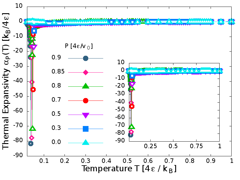
a) b)

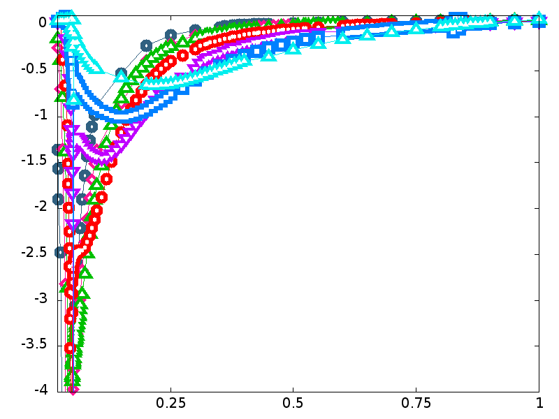
Figure 5: Isobaric thermal expansivity $\alpha_{P}$ calculated as function of $T$. a) We find strong minima at low $T$ for any $P>0$. The minima occur at approximately constant $T$ with an apparent divergence at $Pv_{0}/(4\epsilon)=0.85$ (inset). At higher $P$ the minima loose intensity and occur at lower $T$ as for the maxima of $C_{P}$ (Fig. 4). b) By zooming into the values of $\alpha_{P}$ at intermediate $T$, we find that the strong minima develop very sharp from weak minima at higher $T$. The weak minima merge into the strong minima as the pressure increases.

Next, we calculate the thermal expansivity $\alpha_{P}\equiv(1/\langle V\rangle)(\partial\langle V\rangle/\partial T)_{P}$ along isobars and find extrema (minima) whose behavior is similar to those for $C_{P}$ (Fig. 5). Specifically, we find strong minima at low $T$ and weak mimima at intermediate $T$ that merge to the strong extrema for increasing $P$ before reaching an apparent divergence for $Pv_{0}/(4\epsilon)=0.85$, consistent with the behavior observed for $C_{P}$. The main difference with the results for $C_{P}$ is that the strong extrema of $\alpha_{P}$ are very sharp in $T$. However, both strong and weak extrema of $\alpha_{P}$ occur at approximately the same temperatures as those for $C_{P}$ (Fig. 7). Furthermore, while the weak maxima of $C_{P}$ are observable only for $P<0$, the weak minima of $\alpha_{P}$ can be calculated for any $Pv_{0}/(4\epsilon)\leq 0.7$.

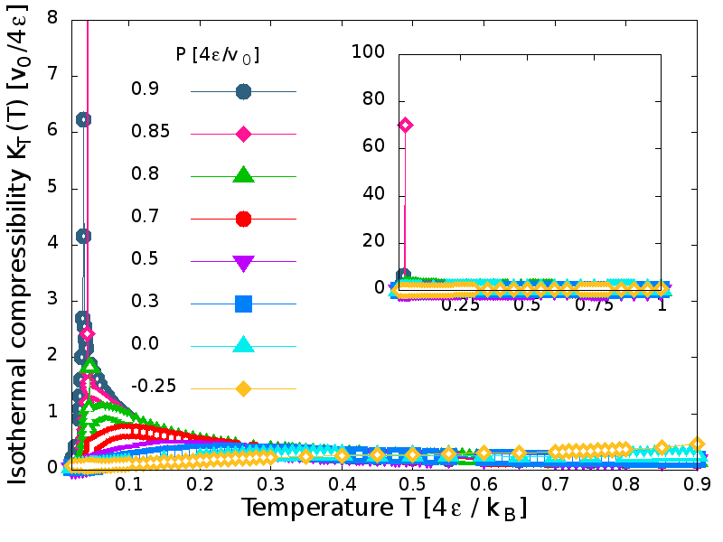
a) b)

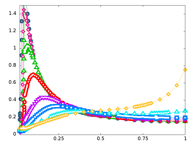
Figure 6: Isothermal compressibility $K_{T}$ calculated along isobars from the fluctuation-dissipation theorem. a) We find, at low $T$ and any $P>0$, maxima that smoothly grows and occur at lower $T$ for higher $P$. b) A closer look at intermediate values $K_{T}(4\epsilon)/v_{0}\simeq 1$ allows us to observe that, as for the case of $\alpha_{P}$ (Fig. 5), there are sharp extrema departing from the smooth (weak) extrema for $0.75\leq Pv_{0}/(4\epsilon)\leq 0.90$. The maxima occur all at approximately the same $T$ and increase in intensity as $P$ approaches $Pv_{0}/(4\epsilon)=0.85$ (inset in a). The weak maxima merge into the strong maxima at $Pv_{0}/(4\epsilon)\simeq 0.85$. Finally, at high $T$ and $0\leq Pv_{0}/(4\epsilon)\leq 0.2$, we find minima in $K_{T}$ occurring at increasing $T$ for increasing $P$.

Finally, we calculate the isothermal compressibility $K_{T}$ from the fluctuation-dissipation theorem, $K_{T}=\langle\Delta V^{2}\rangle/k_{B}TV$, along isobars (Fig. 6). We find strong maxima for $0.7<Pv_{0}/4\epsilon\leq 0.9$ with an apparent divergence at $Pv_{0}/(4\epsilon)=0.85$ and weak maxima for $P>0$. The strong maxima are sharp as for the extrema of $\alpha_{P}$. Furthermore we observe that the weak maxima of $K_{T}$ occur at $T$ higher than the weak extrema of $\alpha_{P}$ and that, approaching $P=0$, they turn into minima. The minima occur at $T$ increasing with $P>0$.

In summary, the fluctuations of enthalpy associated to $C_{P}$, the fluctuations of volume associated to $K_{T}$ and the cross fluctuations of volume and entropy associated to $\alpha_{P}$ increase when $T$ decreases at constant $P$ and display two maxima: a maximum occurring at a $P$-dependent value of $T$, and a strong maximum occurring a very low $T$ that is almost $P$-independent.

The strong maxima appear at the same $T$ where $N_{\rm coop}$ has the largest variation, i.e. where the fluctuations of $N_{\rm coop}$ are maxima. As a consequence, both the volume fluctuations for the Eq.(6), and the enthalpy fluctuation for the Eq.(7) are maxima near the same $T$ Franzese and Stanley (2007b). Therefore, the strong maxima are due to the cooperative rearrangement of the HB network.

On the other hand, the weak maxima at higher temperatures are due to weak volume fluctuations associated to the formation of single HBs, coinciding with the largest variation of $N_{\rm HB}$, as already seen for the water monolayer case Mazza et al. (2011, 2012).

The resulting phase diagram (Fig. 7) of the 3D many-body water closely resemble the one observed for the monolayer case Bianco and Franzese (2014). In the $P$-$T$ phase diagram we find the liquid-to-gas (LG) spinodal at negative pressures defined as the point where $K_{T}$ presents a huge increase and $C_{P}$ has a discontinuous decrease due to the emergence of the gas phase. Above the LG spinodal we find a retracing TMD line that converges at low $P$ toward the TminD line at low $T$, consistent with experimental data Mallamace and et al. (2007) and atomistic simulations Poole et al. (2005). Below the TMD line we find weak extrema at higher $T$ and strong extrema at lower $T$ for the response functions, $C_{P}(T)$, $K_{T}(T)$ and $\alpha_{P}(T)$. While the loci of weak extrema are $P$-dependent and merge at high $P$, the loci of strong extrema are $P$-independent and overlap. The locus of weak maxima of $K_{T}$ converges at lower $P$ toward the locus of minima of $K_{T}$ as observed in atomistic simulations Poole et al. (2005). Furthermore, as can be demonstrated by thermodynamic argument Poole et al. (2005), the locus of minima of $K_{T}$ crosses the turning point of the TMD line, showing that our results are thermodynamically consistent Bianco and Franzese (2014).

All the loci of strong and weak extrema converge toward the same high-$P$ region where they all display a large increase near $Pv_{0}/(4\epsilon)\simeq 0.85$ where they all seem to diverge. As demonstrated by finite size scaling for the case of a monolayer Bianco and Franzese (2014), this finding is consistent with the occurrence of a LLPT ending in a liquid-liquid critical point.

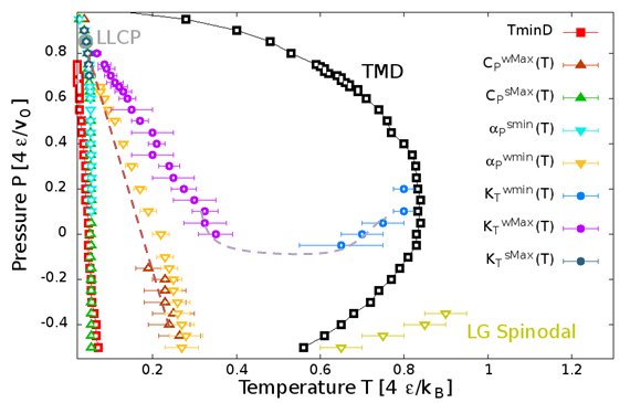
Figure 7: The 3D many-body liquid water phase diagram in the $P$-$T$ plane. Below the temperature of maximum density (TMD) line (black squares) and above the liquid-to-gas (LG) spinodal (green lower triangles) at low $P$ and the temperature of minimum density (TminD) line (red squares), the loci of isobaric weak and strong extrema of, respectively, specific heat $C_{P}^{wMax}$ (red upper triangles with dashed lines), $C_{P}^{sMax}$ (green upper triangles), thermal expansivity $\alpha_{P}^{wmin}$ (yellow lower triangles), $\alpha_{P}^{smin}$ (turquoise lower triangles), and isothermal compressibility $K_{T}^{wMax}$ (purple circles), $K_{T}^{sMax}$ (green circles) cross all at $Pv_{0}/(4\epsilon)\simeq 0.85$, where we estimate the liquid-liquid critical point (LLCP, gray circle). The locus of $K_{T}^{wMax}$ converges toward the locus of isobaric minima $K_{T}^{wmin}$ (blue circles). Dashed lines are guides for the eyes.

V Conclusions

Our analysis shows that the bulk many-body water model reproduces the fluid properties of water in a wide range of pressures and temperatures. Below the liquid gas phase transition and above the liquid-to-gas spinodal in the stretched liquid state at $P<0$, we find the TMD line and, at much lower $T$, the TminD line. The first at atmospheric pressure, corresponding to $P\simeq 0$ in our model, occurs at 277 K, while the second is estimated at a $T=203\pm 5$ K Mallamace et al. (2007). Therefore, the phase diagram we present here goes from the gas to the deep supercooled region of liquid water.

Below the TMD line, we find $P$-dependent extrema of the response functions $C_{P}$, $\alpha_{P}$ and $K_{T}$. While $\alpha_{P}$ has extrema at all the investigated $P$, $C_{P}$ displays $P$-dependent maxima only at negative $P$, while $K_{T}$ only at $P>0$. In particular, the maxima of $K_{T}$ converge toward minima for $P$ approaching 0 and these minima cross the turning point of the TMD line as expected Poole et al. (2005), showing that our results are thermodynamically consistent and similar to those of atomistic models for water Poole et al. (2005); González et al. (2016).

However, our model allows us to simulate in an efficient way supercooled liquid water even at temperatures below the TminD line, an extremely demanding task for atomistic models as a consequence of the glassy slowing down of the dynamics Kesselring et al. (2012, 2013). Thanks to this peculiar property we find that at $Tk_{B}/4\epsilon\simeq 0.035$, below the loci of the $P$-dependent maxima, all the response functions have sharp maxima that have almost no $P$ dependence up to $Pv_{0}/(4\epsilon)\simeq 0.85$. We therefore call these maxima strong and call weak the $P$-dependent maxima. We find that the weak maxima merge with the strong maxima for $Pv_{0}/(4\epsilon)\leq 0.85$.

It is interesting to observe that weak and strong maxima have been found also in the monolayer many-body water model Mazza et al. (2011, 2012); Bianco et al. (2013); Bianco and Franzese (2014) but with an important difference. For the monolayer case the strong maxima of $C_{P}$ are observed also for $P>0$, while for the bulk case they are overshadowed by the strong maxima at $P>0$.

This difference between monolayer and bulk water is consistent with the fact that in the latter the total number of accessible states is much larger. In the case of the monolayer each molecule has four bonding variables with $6^{4}$ accessible configurations de los Santos and Franzese (2011). Instead, for the bulk each molecule has six bonding variables with $6^{6}$ accessible configurations. Therefore, the entropy loss due to the formation of the HB network is much greater for the bulk with respect to the monolayer, consistent with a $C_{P}$ with broader maxima that dominate over the weak maxima.

It is worth noticing that although our prediction of strong and weak maxima for the response functions has not been directly tested in atomistic models, it is perfectly consistent, qualitatively, with the results of atomistic simulations and at the same time with the experimental results Bianco et al. (2013). Furthermore, several atomistic models give hints of more than one maxima in $C_{P}$, showing the line of $P$-dependent $C_{P}$ maxima converging toward the line of $C_{P}$ minima when crossing the point where the TMD line meets the TminD line Poole et al. (2005); González et al. (2016). This convergence of loci of $C_{P}$ maxima, TMD, TminD and $C_{P}$ minima is consistent with the results for the water monolayer Bianco and Franzese (2014) and possibly also with the present results for bulk water.

We find that all the maxima of response functions merge and diverge at $Pv_{0}/(4\epsilon)\simeq 0.85$ and $Tk_{B}/4\epsilon\simeq 0.035$. Therefore we estimate the occurrence of a LLCP at these approximate values. A finite-size analysis, as the one performed for the monolayer case Bianco and Franzese (2014), would be necessary to estimate with larger confidence the LLCP. This analysis could also allows us to study the universality class of the LLCP in bulk. However, such analysis is beyond the scope of the present work.

For $Pv_{0}/(4\epsilon)>0.85$ we find that the maxima of the response functions decrease and occur at lower $T$, consistent with a LLPT with negative slope in the $P$-$T$ plane and ending in the LLCP, as found for the water monolayer Bianco and Franzese (2014).

In conclusion, our results for the bulk many-body water model are consistent with the LLCP scenario for supercooled liquid water Poole et al. (1992). Furthermore, we find properties consistent with those demonstrated in a rigorous way for the many-body water monolayer, including the occurrence of strong and weak maxima for the response functions Bianco and Franzese (2014). Therefore, we can argue that these properties do not originate in the low-dimensionality of the monolayer system, but they are an intrinsic property of the model due to the cooperative contribution to the HB interactions. Because the cooperativity in water is a necessary implication of its peculiar properties Barnes et al. (1979); Guevara-Vela et al. (2016), we argue that our results are relevant for real water.

VI Acknowledgments

V.B. and G.F. acknowledge support from the Austrian Science Fund (FWF) project P 26253-N27 and the Spanish MINECO grant FIS2012-31025 and FIS2015-66879-C2-2-P, respectively.

Appendix A Gas-liquid phase transition

We calculate isobars by applying an annealing protocol. We first simulate a random configuration at high temperature. Next we decrease the temperature and simulate starting from the equilibrated configuration of the previous step. Before reaching the liquid phase, water undergoes a gas-liquid phase transition (Fig. 8) with an abrupt increase of density in the transition from gas to liquid phase.

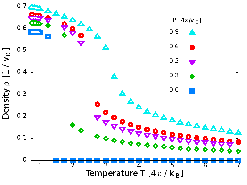
Figure 8: Isobaric variation of the density at high temperatures. There is an abrupt change in the density as the system undergoes the gas-liquid phase transition

Appendix B Error calculation in the specific heat

We made two independent calculations for the specific heat, one using the fluctuation-dissipation (FD) theorem and the other, using its definition as the temperature derivative of the enthalpy (TD). According to Statistical Physics, both results are equal under thermodynamic equilibrium conditions. For this reason, a good test to check whether the system is or is not equilibrated is to compare both results. If the system is well-equilibrated, they must overlap within their error bars.

We calculate average enthalpy $\langle H\rangle$ and fluctuations $\langle\Delta H^{2}\rangle$ from the simulations and estimate the error using the Jackknife method. The method allows us also to estimate the MC correlation time as $\tau^{MC}\sim 256$ MC Steps. As a consequence we estimate that our averages are calculated over $\simeq 400$ independent simulations (Fig. 9).

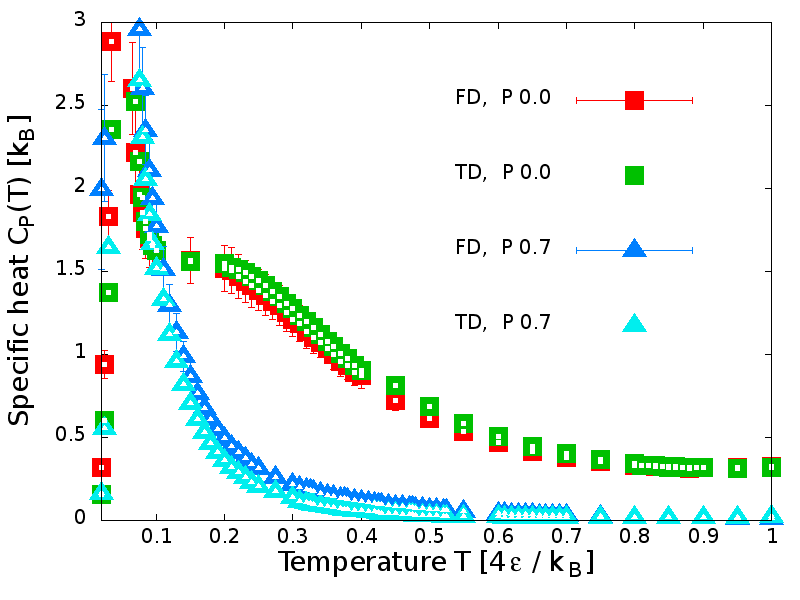
Figure 9: Isobaric specific heat for two cases of high and low pressure. The resulting $C_{P}$ obtained from TD fits within the errorbar of FD

On the one hand, the FD formula for the specific heat $C_{P}$ and its error $\delta C_{P}$ are

$$C_{P}^{FD}=\frac{<\Delta H^{2}>}{k_{B}T^{2}}$$ (9)

$$\delta C_{P}^{FD}=\left|\frac{\partial C_{P}}{\partial\langle\Delta H^{2}\rangle}\right|\delta\Delta H^{2}=\frac{\delta\Delta H^{2}}{k_{B}T^{2}}$$ (10)

On the other hand, the TD formula is

$$C_{P}^{TD}=\frac{\langle H(T)\rangle-\langle H(T-\Delta T)\rangle}{\Delta T}$$ (11)

where we have used the numerical finite differences method. The error for $C_{P}$ in the TD method is

$$\delta C_{P}^{TD}=\frac{\delta\langle H(T)\rangle+\delta\langle H(T-\Delta T)\rangle}{\Delta T}.$$ (12)

References

- Levy and Onuchic (2004) Y. Levy and J. N. Onuchic, Proceedings of the National Academy of Sciences of the United States of America 101, 3325 (2004).
- Franzese et al. (2011) G. Franzese, V. Bianco, and S. Iskrov, “Water at Interface with Proteins,” (2011).
- Bianco et al. (2012) V. Bianco, S. Iskrov, and G. Franzese, “Understanding the role of hydrogen bonds in water dynamics and protein stability,” (2012).
- Bianco and Franzese (2015) V. Bianco and G. Franzese, Phys. Rev. Lett. 115, 108101 (2015).
- Sirovetz et al. (2015) B. J. Sirovetz, N. P. Schafer, and P. G. Wolynes, J. Phys. Chem. B 119, 11416 (2015).
- Mallamace et al. (2016) F. Mallamace, C. Corsaro, D. Mallamace, S. Vasi, C. Vasi, P. Baglioni, S. V. Buldyrev, S.-H. Chen, and H. E. Stanley, Proceedings of the National Academy of Sciences of the United States of America 113, 3159 (2016).
- Johnson et al. (2008) M. E. Johnson, C. Malardier-Jugroot, R. K. Murarka, and T. Head-Gordon, The Journal of Physical Chemistry B 113, 4082 (2008).
- Ngai et al. (2008) K. L. Ngai, S. Capaccioli, and N. Shinyashiki, The Journal of Physical Chemistry B 112, 3826 (2008).
- Mazza and et al. (2011) M. Mazza and et al., Proc. Natl. Acad. Sci. USA 108 (2011).
- Schirò and et al. (2015) G. Schirò and et al., Nat. Commun. 6 (2015).
- Fogarty and Laage (2014) A. Fogarty and D. Laage, The Journal of Physical Chemistry. B 118, 7715 (2014).
- Mallamace et al. (2015) F. Mallamace, C. Corsaro, D. Mallamace, N. Cicero, S. Vasi, G. Dugo, and H. E. Stanley, Frontiers of Physics 10, 1 (2015).
- Chaplin (2006) M. Chaplin, Nature Rev. 7, 861 (2006).
- Debenedetti (1996) P. G. Debenedetti, Metastable Liquids. Concepts and Principles (Princeton University Press, Princeton, NJ, 1996).
- Errington and Debenedetti (2001) J. R. Errington and P. G. Debenedetti, Nature 409, 318 (2001).
- Vega et al. (2009) C. Vega, J. L. F. Abascal, M. M. Conde, and J. L. Aragones, Faraday Discuss 141, 251 (2009).
- Barnes and et al. (1979) P. Barnes and et al., Nature 282 (1979).
- Cruzan and et al. (1996) J. D. Cruzan and et al., Science 271, 59 (1996).
- Perez and et al. (2014) C. Perez and et al., Angew. Chem. 53, 14596 (2014).
- Guevara-Vela and et al. (2016) J. M. Guevara-Vela and et al., Phys. Chem. Chem. Phys. (2016).
- Agapov and et al. (2015) A. L. Agapov and et al., Phys. Rev. E 91, 022312 (2015).
- Kanno and Angell (1979) H. Kanno and C. A. Angell, The Journal of Chemical Physics 70, 4008 (1979).
- Angell et al. (1982) C. A. Angell, W. J. Sichina, and M. Oguni, Journal of Physical Chemistry 86, 998 (1982).
- Poole et al. (1994) P. H. Poole, F. Sciortino, T. Grande, H. E. Stanley, and C. A. Angell, Physical Review Letters 73, 1632 (1994).
- Tanaka (1996) H. Tanaka, Nature 380, 328 (1996).
- Mishima and Stanley (1998) O. Mishima and H. E. Stanley, 392, 164 (1998).
- Soper and Ricci (2000) A. K. Soper and M. A. Ricci, Physical Review Letters 84, 2881 (2000).
- Xu et al. (2005) W.-X. Xu, J. Wang, and W. Wang, Proteins-Structure Function And Genetics 61, 777 (2005).
- Liu et al. (2007) D. Liu, Y. Zhang, C.-C. Chen, C.-Y. Mou, P. H. Poole, and S.-H. Chen, Proceedings of the National Academy of Sciences 104, 9570 (2007).
- Stokely et al. (2010) K. Stokely, M. G. Mazza, H. E. Stanley, and G. Franzese, Proceedings of the National Academy of Sciences of the United States of America 107, 1301 (2010).
- Abascal and Vega (2010) J. L. F. Abascal and C. Vega, The Journal of Chemical Physics 133, 234502 (2010).
- Bertrand and Anisimov (2011) C. E. Bertrand and M. A. Anisimov, The Journal of Physical Chemistry B 115, 14099 (2011).
- Holten et al. (2013) V. Holten, D. T. Limmer, V. Molinero, and M. A. Anisimov, The Journal of Chemical Physics 138, 174501 (2013).
- Pallares et al. (2014) G. Pallares, M. El Mekki Azouzi, M. A. González, J. L. Aragones, J. L. F. Abascal, C. Valeriani, and F. Caupin, Proceedings of the National Academy of Sciences 111, 7936 (2014), http://www.pnas.org/content/111/22/7936.full.pdf .
- Bianco and Franzese (2014) V. Bianco and G. Franzese, Scientific Reports 4, 4440 (2014).
- Soper (2014) A. K. Soper, Nature materials 13, 671 (2014).
- Nilsson and Pettersson (2015) A. Nilsson and L. G. M. Pettersson, Nature communications 6, 8998 (2015).
- Sciortino et al. (2011) F. Sciortino, I. Saika-Voivod, and P. H. Poole, Phys. Chem. Chem. Phys. 13, 19759 (2011).
- Liu et al. (2012) Y. Liu, J. C. Palmer, A. Z. Panagiotopoulos, and P. G. Debenedetti, The Journal of Chemical Physics 137, 214505 (2012).
- Palmer et al. (2013) J. C. Palmer, R. Car, and P. G. Debenedetti, Faraday Discuss. 167, 77 (2013).
- Poole et al. (2013) P. H. Poole, R. K. Bowles, I. Saika-Voivod, and F. Sciortino, The Journal of Chemical Physics 138, 34505 (2013).
- Palmer et al. (2014) J. C. Palmer, F. Martelli, Y. Liu, R. Car, A. Z. Panagiotopoulos, and P. G. Debenedetti, Nature 510, 385 (2014).
- Smallenburg and Sciortino (2015) F. Smallenburg and F. Sciortino, Physical review letters 115, 015701 (2015).
- Speedy (1982) R. J. Speedy, The Journal of Physical Chemistry 86, 982 (1982).
- Sastry et al. (1996) S. Sastry, P. G. Debenedetti, F. Sciortino, and H. E. Stanley, Physical Review E 53, 6144 (1996).
- Poole et al. (1992) P. Poole, F. Sciortino, U. Essmann, and H. Stanley, Nature 360, 324 (1992).
- Angell (2008) C. A. Angell, Science 319, 582 (2008).
- Fuentevilla and Anisimov (2006) D. A. Fuentevilla and M. A. Anisimov, Phys. Rev. Lett. 97, 195702 (2006).
- Franzese et al. (2003) G. Franzese, M. I. Marqués, and H. E. Stanley, Physical Review E 67, 11103 (2003).
- Franzese and Stanley (2002) G. Franzese and H. Stanley, J. Phys. Condes. Matter 14, 2201 (2002).
- Franzese and Stanley (2007a) G. Franzese and H. Stanley, J. Phys.: Condes. Matter 19 (2007a).
- Franzese and Stanley (2007b) G. Franzese and H. E. Stanley, Journal of Physics: Condensed Matter 19, 205126 (2007b).
- de los Santos and Franzese (2011) F. de los Santos and G. Franzese, The Journal of Physical Chemistry B (2011), 10.1021/jp206197t.
- Vilanova and Franzese (2011) O. Vilanova and G. Franzese, arXiv:1102.2864 (2011).
- Note (1) We adopt two-axis periodic boundary conditions in such a way to be able to perform consistent checks with previous results for the monolayer model.
- Mazza et al. (2009) M. G. Mazza, K. Stokely, E. G. Strekalova, H. E. Stanley, and G. Franzese, Special issue based on the Conference on Computational Physics 2008 - CCP 2008, Computer Physics Communications 180, 497 (2009).
- Stanley and Teixeira (1980) H. E. Stanley and J. Teixeira, The Journal of Chemical Physics 73, 3404 (1980).
- Mazza et al. (2011) M. G. Mazza, K. Stokely, S. E. Pagnotta, F. Bruni, H. E. Stanley, and G. Franzese, Proceedings of the National Academy of Sciences 108, 19873 (2011).
- Mazza et al. (2012) M. G. Mazza, K. Stokely, H. E. Stanley, and G. Franzese, The Journal of Chemical Physics 137, 204502 (2012).
- Mallamace and et al. (2007) F. Mallamace and et al., Proc Natl Acad Sci USA 104, 18387 (2007).
- Poole et al. (2005) P. H. Poole, I. Saika-Voivod, and F. Sciortino, J. Phys.: Condens. Matter 17, L431 (2005).
- Mallamace et al. (2007) F. Mallamace, C. Branca, M. Broccio, C. Corsaro, C.-Y. Mou, and S.-H. Chen, Proceedings of the National Academy of Sciences of the United States of America 104, 18387 (2007).
- González et al. (2016) M. A. González, C. Valeriani, F. Caupin, and J. L. F. Abascal, The Journal of Chemical Physics 145, 054505 (2016), http://dx.doi.org/10.1063/1.4960185.
- Kesselring et al. (2012) T. Kesselring, G. Franzese, S. Buldyrev, H. Herrmann, and H. E. Stanley, Nature Scientific Reports 2, 474 (2012).
- Kesselring et al. (2013) T. Kesselring, E. Lascaris, G. Franzese, S. V. Buldyrev, H. Herrmann, and H. E. Stanley, Journal of Physical Chemistry 138, 244506 (2013), arXiv:1302.1894 [cond-mat.soft] .
- Bianco et al. (2013) V. Bianco, M. G. Mazza, K. Stokely, , F. Bruni, H. E. Stanley, and G. Franzese, in Proceedings of “Symposium on the Fragility of Glass-formers: A Conference in Honor of C. Austen Angell”, edited by R. Ganapathy, A. L. Greer, K. F. Kelton, and S. Sastry (2013).
- Barnes et al. (1979) P. Barnes, J. L. Finney, J. D. Nicholas, and J. E. Quinn, Nature 282, 459 (1979).
- Guevara-Vela et al. (2016) J. M. Guevara-Vela, E. Romero-Montalvo, V. A. Mora-Gomez, R. Chavez-Calvillo, M. Garcia-Revilla, E. Francisco, A. Martin Pendas, and T. Rocha-Rinza, Physical Chemistry Chemical Physics (2016), 10.1039/C6CP00763E.