Scaling of Navier-Stokes trefoil reconnection

Abstract

Perturbed, helical trefoil vortex knots and a set of anti-parallel vortices are examined numerically to identify the scaling of their helicity and vorticity norms during reconnection. For the volume-integrated enstrophy $Z=\int_{\mathbb{T}_{\ell}^{3}}\omega^{2}dV$, a new scaling regime is identified for both configurations where as the viscosity $\nu$ changes, all $\sqrt{\nu}Z(t)$ cross at $\nu$-independent times $t_{x}$, identified as when the first reconnection events end. Self-similar linear collapse of $B_{\nu}(t)=(\sqrt{\nu}Z)^{-1/2}$ can be found for $t\lesssim t_{x}$ by linearly extrapolating $B_{\nu}(t)$ to zero at critical times $T_{c}(\nu)$, then plotting $(T_{c}(\nu)-t_{x})\bigl{(}B_{\nu}(t)-B_{x}\bigr{)}$ where $B_{x}=B_{\nu}(t_{x})$. The size $\ell^{3}$ of the periodic domains must be increased as $\nu$ is decreased to maintain this scaling as implied by known Sobolev space bounds. The anti-parallel calculations show that the linear collapse of $B_{\nu}(t)$ begins with a quick, viscosity-independent exchange of the circulation $\Gamma$ between the original vortices and the new vortices. Up to and after the trefoil knots’ first reconnection at time $t_{x}$, their helicity ${\cal H}$ is preserved, validating the experimental centreline helicity observation of Scheeler et al. (2014a). Because the cubic Navier-Stokes velocity norm $\|{u}\|_{L^{3}}$ barely changes and the Navier-Stokes $\|\omega\|_{\infty}$ are bounded by the Euler values, these flows are never singular. Despite this, the Navier-Stokes $Z$ can, for a brief period, grow faster than the Euler $Z$ and the following increase in the viscous energy dissipation rate $\epsilon=\nu Z$ shows $\nu$-independent convergence at $t\approx 2t_{x}$. Taken together, these results could be a new paradigm whereby smooth solutions without singularities or roughness could generate a $\nu\to 0$ dissipation anomaly (finite dissipation in a finite time) as $\ell\to\infty$, as seen in physical turbulent flows.

1 Background

Two long-standing questions about nonlinear growth in fluid turbulence are these: Does hydrodynamic helicity have a role in controlling nonlinearity that is analogous to the role of the helicity of magnetic systems (Moffatt, 2014)? And can there be smooth nonlinear growth whose scaling is consistent with the formation of a Navier-Stokes dissipation anomaly? That is, can there be finite energy dissipation in a finite time as the viscosity $\nu\to 0$? The first question needs revisiting due to the recent vortex knot reconnection experiments of Scheeler et al. (2014a) that observed complete reconnections, indicating strong nonlinearities, while simultaneously retaining strong helicity that could have suppressed that growth. Inspired by those experiments, this paper gains insight into both questions using new high-resolution simulations of reconnecting trefoil vortex knots and anti-paralllel vortices.

The dissipation anomaly question is addressed by considering the following dichotomy. Vassilicos (2015) quotes several sources to conclude that there is a consensus that whenever an energy cascade is observed, the energy dissipation rate $\epsilon=\nu Z$ is independent of $\nu$, where $Z(t)$ is the volume-integrated enstrophy (3). This contrasts with the mathematics that shows that unless there are singularities, $\nu\to 0$ finite dissipation cannot form when the domain is fixed (Constantin, 1986). Could the unexpected preservation of helicity during the reconnection of the experimental trefoil knot of Scheeler et al. (2014a) provide clues to resolving this dichotomy?

The trefoils being simulated have the topology of a (2,3) knot, are inherently helical and evolve as self-reconnecting, doubly-looped rings. As described in section 2, to properly reproduce the single, dominant reconnection event of the experimental trefoils, perturbations are needed to break the three-fold symmetry of an ideal trefoil. The resulting initial state is given in figure 1 and once this perturbed state was generated, the first task was to establish the range of viscosities and thicknesses that could be run using comparisons of peak vorticities $\|\omega\|_{\infty}$ for different resolutions and domains as in figures 2 and evolving enstrophy spectra $Z(k,t)$ as in figure 3. This initial analysis also provided preliminary trends for how trefoil reconnnection events can be suppressed, enhanced and develop signs of self-similarity,

The next task would have been to examine whether the Scheeler et al. (2014a) claim that helicity can be preserved during the first reconnection, which is now confirmed in figure 11,

However, the helicity analysis was soon overshadowed by the identification of new self-similar scaling regime for the evolution of the volume-integrated enstrophy $Z(t)$ during the first reconnection. The kernel of this scaling regime is using $\sqrt{\nu}Z(t)$, $\nu$ viscosity, instead of the expected dissipation rate scaling of $\epsilon(t)=\nu Z(t)$, and was first identified using figure 4a. After some exploration it was found to manifests itself more completely in figure 5 as a viscosity-independent, linear collapse of $(\sqrt{\nu}Z(t))^{-1/2}$ until the first reconnection ends at $t=t_{x}$. This scaling has probably not been noticed because it requires increasing the size of the domain $\ell$ as $\nu\to 0$ due to mathematical bounds upon the growth of higher-order norms in finite periodic domains most of the fluids community is not familiar with. This behaviour could apply to all strong reconnection events as the collapse is also found for the new anti-parallel vortex reconnection calculations in figure 8. Its importance is that this scaling regime could be a precursor to the formation of a $\nu\to 0$, $\ell\to\infty$ dissipation anomaly from smooth solutions at later times, as demonstrated by the energy dissipation rates $\epsilon(t)=\nu Z(t)$ plotted in figure 4b.

It is important to place these two surprising results, helicity preservation and the new $\sqrt{\nu}Z(t)$ enstrophy scaling, in the context of what is already known from simulations about the role of helicity and known results from applied analysis of the Navier-Stokes about what could potentially bound the growth of the enstrophy $Z(t)$.

If the initial state is a collection of random large-scale helical Fourier modes, simulations show that the onset of turbulence can be delayed. However, the subsequent decay is similar to what non-helical initial conditions generate (Polifke et al., 1989). Another Fourier approach is to insert anisotropic modes or forcing at intermediate wavenumbers to determine the influence of the sign of helicity upon the energy cascade (Biferale & Kerr, 1995; Sahoo et al., 2015). Helicity is also a continuum measure of the topology of the vortices (Moffatt & Ricca, 1992), so can serve as a diagnostic for changes in the topology. However, up to now this use of helicity has been limited because the configurations that are easy to construct, such as anti-parallel and orthogonal pairs, have zero or weak helicity. The only calculations with some helicity have used skewed initial states, either random (Holm & Kerr, 2007) or vortical (Kimura & Moffatt, 2014). These have reinforced the perspective that helicity tends to suppress nonlinearity before it disappears. This question will be revisited in section 6.2 with respect to the generation of negative helicity.

Based upon that experience, the experimental observation that a trefoil’s helicity can be preserved during topology changing reconnections was unexpected. Instead, it seems that the trefoil’s self-linking helicity can be converted directly into the mutual helicity of new linked rings during reconnection, as suggested by Laing et al. (2015).

Regularity questions and results arise due to the $\nu\to 0$, viscosity-independent convergence of the scaled enstrophy $\sqrt{\nu}Z(t)$ at $t=t_{x}\approx 40$ in figure 4 and the circulation exchange $\epsilon_{\Gamma}(t)$ (29) at $t=t_{\Gamma}\approx 16.5$ in figure 8. These imply respectively that $Z(t_{x})\sim\nu^{-1/2}$ (35) and that the velocity second-derivatives (34) in $\epsilon_{\Gamma}$ go as $\nu^{-3/2}$. In contrast to these trends for growth as $\nu\to 0$, the two diagnostics primarily used for showing regularity of the Navier-Stokes equation as defined by the Clay prize problem (Fefferman, 2000), imply regularity for all time. One diagnostic is the Navier-Stokes vorticity maximum $\|\omega\|_{\infty}$ (10), whose growth is bounded by the regular Euler values in figure 2. The other diagnostic is the cubic velocity norm $\|{u}\|_{L^{3}}$ (6). By Escauriaza et al. (2003), there can be singularities of Navier-Stokes only if $\|{u}\|_{L^{3}}$ is singular and instead, figure 11c shows that $\|{u}\|_{L^{3}}$ is nearly independent of the viscosity and time. Is there mathematics that might be consistent with these opposing trends?

The mathematical result most relevant to these calculations is a proof for how regular, non-singular Euler solutions can bound Navier-Stokes solutions in fixed domains $\ell^{3}$ as $\nu\to 0$ (Constantin, 1986). What was shown is that so long as solutions under Euler are bounded, critical viscosities $\nu_{s}$ can be found for each $\|{u}\|_{H^{s}}$ norm such that, for any $\nu<\nu_{s}$, the Navier-Stokes solutions will be bounded by functions of the regular Euler solutions. This result is largely unknown in the fluids community and comes close to saying that a $\nu\to 0$ dissipation anomaly cannot form. This is because in fixed domains these bounds would preclude the viscosity-independent convergence of both $\sqrt{\nu}Z(t)$ and $\epsilon=\nu Z(t)$ in figure 4. Section 3.1 will show how this constraint can be relaxed by increasing $\ell$ as $\nu$ decreases, potentially allowing a $\nu\to 0$ dissipation anomaly to form. The remaining mathematical caveats upon that statement are discussed in sections 7 and 8.

Is the trefoil an appropriate configuration for investigating fundamental questions about the regularity of the Navier-Stokes equations? In fact, the trefoil is well-suited for these questions for the following reasons. First, a trefoil self-reconnects. Second, unlike other configurations such as initially anti-parallel or orthogonal vortices, most of a trefoil’s velocity and vorticity norms are finite in an infinite domain, including the enstrophy $Z$ (3) and the helicity ${\cal H}$ (4). Third, opposing the tendency to self-reconnect, the trefoil knots can be used to investigate how helicity suppresses nonlinearities because the initial helicity is unusually close to the upper bound defined by the energy and enstrophy, ${\cal H}\leq(2EZ)^{1/2}$. Fourth, it can be simulated in a periodic box, making detailed Fourier analysis using Sobolev norms possible.

This paper is organised as follows. After introducing the equations, diagnostics and initialisation, illustrated for the Q-trefoil in figure 1, there is a step-by-step description of how the $\sqrt{\nu}Z(t)$ scaling for the Q-trefoil in figure 4a can be transformed into a viscosity-independent, linear collapse of $(\sqrt{\nu}Z(t))^{-1/2}$ up to a time of $t=t_{x}\approx 40$ in figure 5, including the mathematics that underlies why the domain size $\ell$ must be increased as the viscosity $\nu$ is decreased. This is the first major result and is not limited to trefoils, as shown by new anti-parallel calculations where this scaling begins with a spurt of circulation exchange and ends when the first reconnection completes. For the trefoils, vorticity isosurfaces at $t=31$ and $t=45$ also show that $t_{x}\approx 40$ is when its first reconnection ends. Later in time, for $t>t_{x}$, the trefoil’s enstrophy growth increases until a finite, $\nu$-independent dissipation rate $\epsilon=\nu Z$ forms at $t\approx 2t_{x}$ in a manner consistent with the formation of a dissipation anomaly. The second major result is confirmation of the experimental preservation of the trefoil helicity ${\cal H}$ to about $1.5t_{x}$, after the first reconnection ends, including cases with a core radius similar to the latest experiments (Scheeler et al., 2014a). The two regularity diagnostics with the same dimensions as ${\cal H}^{1/2}$, $\|{u}\|_{L^{3}(\mathbb{T}_{\ell}^{3})}$ and $\|{u}\|_{\dot{H}^{1/2}(\mathbb{T}_{\ell}^{3})}$, are also plotted and discussed. Finally, figure 12 shows that the self-similar scaling of the growth of enstrophy $Z$ continues to extremely small viscosities despite the empirical evidence in figure 2 that $\|\omega\|_{\infty}$ is bounded by the regular Euler solutions.

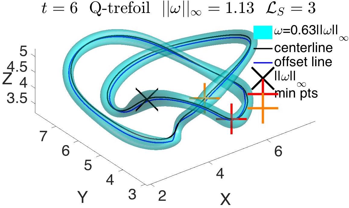
Figure 1: Vorticity isosurface plus two closed vortex lines of the perturbed trefoil vortex at $t=6$, not long after initialisation. One vortex line has been seeded at $\|\omega\|_{\infty}$ and the other a bit offset, allowing the self-linking ${\cal L}_{S}$ to be calculated using (15) giving ${\cal L}_{S}=3$, which can be split (13) into a writhe of $W\!r=3.15$ and a twist of $T\!w=-0.15$. X is the location of $\|\omega\|_{\infty}$ and the seed for the black vortex line. The red and yellow + are the points of closest approach of the two loops of the trefoil and where reconnection will begin.

1.1 Equations and continuum diagnostics

The governing equations for the simulations in this paper will be the incompressible Navier-Stokes equations on the toris $\mathbb{T}_{\ell}^{3}$, that is a periodic box with volume ($V=\ell^{3}$).

$$\begin{array}[]{r}\mbox{\boldmath$u$}_{t}-\nu\mbox{\boldmath$\triangle$}\mbox{\boldmath$u$}+(\mbox{\boldmath$u$}\mbox{\boldmath$\cdot$}\nabla)\mbox{\boldmath$u$}+\nabla p=0\\ \nabla\mbox{\boldmath$\cdot$}\mbox{\boldmath$u$}=0\end{array}\Bigr{\}}\quad{\rm in}~{}\mathbb{R}^{3}\times(-\infty,T)$$ (1)

The equations for the densities of the energy, enstrophy and helicity, $e=\mbox{$\frac{1}{2}$}|\mbox{\boldmath$u$}|^{2}$, $|\mbox{\boldmath$\omega$}|^{2}$ and $h=\mbox{\boldmath$u$}\cdot\mbox{\boldmath$\omega$}$ respectively are (with their volume-integrated norms):

$$\frac{\partial e}{\partial t}+({\mbox{\boldmath$u$}}\cdot\nabla)e=-\nabla\cdot(\mbox{\boldmath$u$}p)+\nu\triangle e-\underbrace{\nu(\nabla\mbox{\boldmath$u$})^{2}}_{\epsilon={\rm dissipation}},\qquad E=\mbox{$\frac{1}{2}$}\int\mbox{\boldmath$u$}^{2}dV\,.$$ (2)

$$\frac{\partial|\mbox{\boldmath$\omega$}|^{2}}{\partial t}+({\mbox{\boldmath$u$}}\cdot\nabla)|\mbox{\boldmath$\omega$}|^{2}=\underbrace{2\mbox{\boldmath$\omega$}\mbox{\boldmath$S$}\mbox{\boldmath$\omega$}}_{Z_{p}={\rm production}}+\nu\triangle|\mbox{\boldmath$\omega$}|^{2}-\underbrace{2\nu(\nabla\mbox{\boldmath$\omega$})^{2}}_{\epsilon_{\omega}=Z-{\rm dissipation}},\qquad Z=\int\mbox{\boldmath$\omega$}^{2}dV\,.$$ (3)

$$\frac{\partial h}{\partial t}+({\mbox{\boldmath$u$}}\cdot\nabla)h=\underbrace{-\mbox{\boldmath$\omega$}\cdot\nabla\Pi}_{\omega-{\rm transport}}+\underbrace{\nu\mbox{\boldmath$\triangle$}h}_{\nu-{\rm transport}}-\underbrace{2\nu{\rm tr}(\nabla\mbox{\boldmath$\omega$}\cdot\nabla\mbox{\boldmath$u$}^{T})}_{\epsilon_{h}={\cal H}-{\rm dissipation}}\qquad{\cal H}=\int\mbox{\boldmath$u$}\cdot\mbox{\boldmath$\omega$}dV\,,$$ (4)

where $\mbox{\boldmath$\omega$}=\nabla\times\mbox{\boldmath$u$}$ is the vorticity vector and $\Pi=p-\mbox{$\frac{1}{2}$}\mbox{\boldmath$u$}^{2}\neq p_{h}$ (pressure head $p_{h}=p+\mbox{$\frac{1}{2}$}\mbox{\boldmath$u$}^{2}$).

The numerical method will be a 2/3rds-dealiased pseudo-spectral code with a very high wavenumber cut-off filter (Kerr, 2013a).

The inviscid ($\nu=0$) invariants are the global energy $E$ and helicity ${\cal H}$ (Moffatt, 1969), plus the circulations $\Gamma_{i}$ about the vortices

$$\Gamma_{i}=\oint\mbox{\boldmath$u$}_{i}\cdot d\mbox{\boldmath$r$}_{i}\quad{\rm where}\quad\mbox{\boldmath$r$}_{i}~{}~{}\mbox{is a closed loop about trajectories}~{}~{}{\mbox{\boldmath$x$}_{i}\in\cal C}_{i}(t)\,.$$ (5)

The initial trajectories $\mbox{\boldmath$x$}_{i}\!\in\!{\cal C}_{i}(0)$ were used to map vorticity onto the mesh and for the $\nu\neq 0$ anti-parallel reconnection, figure 8 uses the symmetry plane diagnostics $\Gamma_{y}(t)$, $\Gamma_{z}(t)$ (28) and $\epsilon_{\Gamma}$ (29) to show the scaling of the reconnection as it begins.

Since the energy in all of the simulations barely decays and the circulation of the trefoil vortex is difficult to determine, changes in the global helicity ${\cal H}$, which has the same dimensional units as the circulation-squared and can be of either sign, has a greater role in characterising the temporal evolution. Furthermore, the sign of the local helicity density $h$ can grow, decrease and even change due to both the $\omega$-transport term along the vortices and the viscous terms in (4) (Biferale & Kerr, 1995). The evolution of the enstrophy $Z$ (3) is simpler as its production term $Z_{p}$ is predominantly positive and its dissipation term is strictly negative-definite.

In addition to $E$, ${\cal H}$ and $Z$, the characterisation of the temporal evolution will use a few volume-integrated versions of the Lebesgue measures and Sobolev-$\dot{H}$ norms. Volume-integrated norms $\mathbb{T}_{\ell}^{3}$ of the periodic $\ell^{3}$ computational domains are used instead of the more common volume-averaged versions so that calculations using different $\ell$ can be compared to each other and to mathematical results for whole space, that is in $\mathbb{R}^{3}=\mathbb{T}^{3}_{\infty}$. The relationships between the volume-integrated $\|{u}\|_{L^{p}(\mathbb{T}_{\ell}^{3})}$ and the volume-averaged $\|{u}\|_{L^{p}}$ Lebesgue measures are:

$$\|{u}\|_{L^{p}(\mathbb{T}_{\ell}^{3})}=\left(\int_{\mathbb{T}_{\ell}^{3}}d\Omega|\mbox{\boldmath$u$}|^{p}\right)^{1/p}=\ell^{3/p}\left(\frac{1}{V}\int_{V=\mathbb{T}_{\ell}^{3}}d\Omega|\mbox{\boldmath$u$}|^{p}\right)^{1/p}=\ell^{3/p}\|{u}\|_{L^{p}}\,.$$ (6)

Using $\hat{\mbox{\boldmath$u$}}(\mbox{\boldmath$k$})$ as the Fourier transform of $\mbox{\boldmath$u$}(\mbox{\boldmath$x$})$, the volume-integrated Sobolev-${\dot{H}}^{s}$ norms $\|{u}\|_{\dot{H}^{s}(\mathbb{T}_{\ell}^{3})}$ are summed over the $\mbox{\boldmath$k$}=\mbox{\boldmath$j$}\Delta k$, where the $\mbox{\boldmath$j$}\!\in\!\mathbb{Z}^{3}$ are the 3D integers and $\Delta k=2\pi/\ell$. The correspondence between the $\|{u}\|_{\dot{H}^{s}(\mathbb{T}_{\ell}^{3})}$ and the averaged $H^{s}$ norms is:

$$\|{u}\|_{\dot{H}^{s}(\mathbb{T}_{\ell}^{3})}=\left(\sum_{\mbox{\boldmath$j$}}\frac{|\mbox{\boldmath$k$}|^{2s}|}{\Delta k^{3}}\hat{\mbox{\boldmath$u$}}(\mbox{\boldmath$k$})|^{2}\right)^{1/2}\!=\left(\frac{\ell}{2\pi}\right)^{3/2}\left(\sum_{\mbox{\boldmath$j$}}|\mbox{\boldmath$k$}|^{2s}|\hat{\mbox{\boldmath$u$}}(\mbox{\boldmath$k$})|^{2}\right)^{1/2}\!=\left(\frac{\ell}{2\pi}\right)^{3/2}\|{u}\|_{\dot{H}^{s}}\,.$$ (7)

The standard $H^{s}$ Sobolev-norms with a pre-factor of $1+k^{2}+\dots+k^{2s}$ are not being used, except when referencing literature that uses the $H^{s}$ norms. To be dimensionally consistent this would have to be a sum of $(k/k_{0})^{m}$ with $k_{0}\sim\ell^{-1}$.

The relationships between the periodic volume-integrated norms on $\mathbb{T}_{\ell}^{3}$ as $\ell\to\infty$ and the $\mathbb{R}^{3}$ norms over whole space are

$$\lim_{\ell\to\infty}\|{u}\|_{L^{p}(\mathbb{T}_{\ell}^{3})}=\|{u}\|_{L^{p}(\mathbb{R}^{3})}=\left(\int_{\mathbb{R}^{3}}d\Omega|\mbox{\boldmath$u$}|^{p}\right)^{1/p}\quad{\rm with}\quad L^{(3)}_{\ell}=\|{u}\|_{L^{3}(\mathbb{T}^{3}_{\ell})}$$ (8)

and

$$\lim_{\ell\to\infty}\|{u}\|_{\dot{H}^{s}(\mathbb{T}_{\ell}^{3})}=\|{u}\|_{\dot{H}^{s}(\mathbb{R}^{3}_{k})}=\left(\int_{\mathbb{R}^{3}_{k}}d^{3}k|\mbox{\boldmath$k$}|^{2s}|\hat{\mbox{\boldmath$u$}}(\mbox{\boldmath$k$})|^{2}\right)^{1/2}\quad{\rm with}\quad\dot{H}^{(1/2)}_{\ell}=\|{u}\|_{\dot{H}^{1/2}(\mathbb{T}_{\ell}^{3})}\,.$$ (9)

Besides the volume-integrated enstrophy $Z=\|{\omega}\|_{L^{0}_{\ell}}^{2}=\|{u}\|_{\dot{H}^{1}}^{2}$ (3,6,7), the other significant vorticity diagnostic will be the maximum of vorticity

$$\|\mbox{\boldmath$\omega$}\|_{\infty}=\|\mbox{\boldmath$\omega$}\|_{L^{\infty}}=\sup|\mbox{\boldmath$\omega$}|\,.$$ (10)

Its time integral will bound any property (Beale et al., 1984) in the sense that:

$${\rm Given}\quad I(T)=\int_{0}^{T}\|\omega\|_{\infty}dt<\infty\quad{\rm then}\quad\|{u(T)}\|_{L^{p}}\leq\|{u(0)}\|_{L^{p}}\exp\bigl{(}C_{p}(\ell)I(T)\bigr{)}\,.$$ (11)

However, this leaves open what the $\ell$ dependence of $C_{p}$ is as $\ell$ increases. For example, if one takes the standard Hölder inequality $\|{\omega}\|_{L^{p}}\leq\tilde{C}_{p}\|{\omega}\|_{L^{p+1}}$, with $\tilde{C}_{p}$ independent of $\ell$, then by (6) and using induction to form a constant $\tilde{C}_{2\infty}$, the volume-integrated enstrophy $Z$ is bounded from above as

$$Z=\|{\omega}\|_{L^{2}(\mathbb{T}_{\ell}^{3})}^{2}=\ell^{3}\|{\omega}\|_{L^{2}}^{2}{}\leq\tilde{C}_{2\infty}\ell^{3}\|{\omega}\|_{\infty}^{2}\,,$$ (12)

which includes the volume as $\ell^{3}$.

The behaviour of the scaled helicity ${\cal H}^{(1/2)}$ (4) and its two partners, the cubic velocity norm $L^{(3)}_{\ell}$ (8) and $\dot{H}^{(1/2)}_{\ell}$ (9) are given in figure 11. All three of these diagnostics have the same units as the circulation: $[\Gamma]=[L^{2}/T]$ and both $L^{(3)}_{\ell}$ and $\dot{H}^{(1/2)}_{\ell}$ have been used to improve our understanding of the regularity of the Navier-Stokes equations (Escauriaza et al., 2003; Doering, 2009; Seregin, 2011). Section 4.1 on applications of Leray (1934) scaling discusses $L^{(3)}_{\ell}$ which is currently the most refined upper bound on Navier-Stokes regularity, along with a possible origin for the $\sqrt{\nu}Z(t)$ scaling. The norm $\dot{H}^{(1/2)}_{\ell}$ is discussed at the end of section 6.

1.2 Vortex lines and linking numbers

The role of the helicity ${\cal H}$ in understanding the trefoil calculations is two-fold. One role is as a constraint upon the growth of nonlinearity in the continuum, the other is to provide a qualitative picture of how the topology can change using the linking numbers. For the continuum equations, ${\cal H}$ is the volume-integral of the helicity density $h=\mbox{\boldmath$u$}\cdot\mbox{\boldmath$\omega$}$ and is conserved by the inviscid equations, with $h$ governed by (4). In a three-dimensional turbulent flow, the kinetic energy cascades overwhelmingly to small scales. In contrast, $h$ can move to both large and small scales.

While the global helicity ${\cal H}$ could in principle be estimated topologically by summing contributions from selected vortex trajectories, in this paper only a few of these trajectories are identified. The topological properties of these trajectories are determined to provide a qualitative picture of the changes to the vortex structures during reconnection that can be used for determining timescales for comparisons with the trefoil experiments (Kleckner & Irvine, 2013; Scheeler et al., 2014a).

When the vortices are distinct, this topological helicity ${\cal H_{L}}$ can in principle be formed using the circulations $\Gamma_{i}$ about the vortex trajectories ${\cal C}_{i}(t)$ (5), the linking numbers ${\cal L}_{ij}$ between all vortices and the integer self-linking numbers of individual closed loops

$${\cal L}_{Si}=W\!r_{i}+T\!w_{i}\,,$$ (13)

where ${\cal L}_{Si}$ is a sum of the non-integer writhe and twist $W\!r_{i}$ and $T\!w_{i}$ (Moffatt & Ricca, 1992). By assigning circulations $\Gamma_{i}$ to the vortices and summing one can determine the global helicity ${\cal H}$ (Moffatt & Ricca, 1992).

$${\cal H_{L}}=\sum_{ij}\Gamma_{i}\Gamma_{j}{\cal L}_{ij}+\sum_{i}\Gamma_{i}^{2}{\cal L}_{S_{i}}\,.$$ (14)

The tool used to determine the writhe, direct self-linking and intervortex linking for the selected vortex lines in figures 1, 9 and 10 is a regularised Gauss linking integral about two loops $\mbox{\boldmath$x$}_{i,j}\in{\cal C}_{i,j}$

$${\cal L}_{ij}=\sum_{ij}\frac{1}{4\pi}\oint_{{\cal C}_{i}}\oint_{{\cal C}_{j}}\frac{(d\mbox{\boldmath$x$}_{i}\times d\mbox{\boldmath$x$}_{j})\cdot(\mbox{\boldmath$x$}_{i}-\mbox{\boldmath$x$}_{j})}{(|\mbox{\boldmath$x$}_{i}-\mbox{\boldmath$x$}_{j}|^{2}+\delta^{2})^{1.5}}\,.$$ (15)

The regularisation of the denominator using $\delta$ has been added for determining the writhe when $i=j$ (Calugareanu, 1959; Moffatt & Ricca, 1992). The self-linking numbers ${\cal L}_{Si}$ can be determined directly using $\delta=0$ by defining the edges of vortex ribbons from two parallel trajectories within the vortex cores, as illustrated in figure 1. For determining the intervortex linking numbers with $i\neq j$, $\delta=0$.

To determine these linking numbers and provide qualitative comparisons with the experimental vortex lines (Kleckner & Irvine, 2013; Scheeler et al., 2014a), vortex lines $\mbox{\boldmath$x$}_{j}(s)$ were identified by solving the following ordinary differential equation,

$$\frac{d\mbox{\boldmath$x$}_{j}(s)}{ds}=\mbox{\boldmath$\omega$}(\mbox{\boldmath$x$}_{j}(s))\,.$$ (16)

This can be easily solved using the Matlab streamline function, which includes a function for interpolating the vorticity vector field $\mbox{\boldmath$\omega$}(\mbox{\boldmath$x$}_{j})$ from the mesh, onto the lines. The seeds for solving (16) were chosen from the positions around, but not necessarily at, local vorticity maxima.

2 Initialisation and domain

Cases	Size $\ell$	i-Mesh	$r_{0}$	$\omega_{\rm in}$	$k_{f}$	$r_{e}$	$\omega_{0}$	$Z_{0}$	$E_{0}$	$\nu$	f-mesh
P	$4\pi$	$128^{3}$	0.33	0.6	8.4	0.56	0.5	$2.68$	0.67	2.5e-4:1.25e-4	$512^{3}$
P	$4\pi$	$128^{3}$	0.33	0.6	8.4	0.56	0.5	$2.68$	0.67	6.25e-5:3.125e-5	$1024^{3}$
P	$6\pi$	$256^{3}$	0.33	0.6	8.4	0.56	0.5	$2.68$	0.72	1.56e-5:7.8e-6	$2048^{3}$
Q	$3\pi$	$128^{3}$	0.25	1.26	11.9	0.40	1	$5.48$	0.96	5e-4	$512^{3}$
Q	$3\pi$	$128^{3}$	0.25	1.26	11.9	0.40	1	$5.48$	0.96	2.5e-4:6.25e-5	$1024^{3}$
Q	$4\pi$	$128^{3}$	0.25	1.26	11.9	0.40	1	$5.29$	0.85	5e-4:1.25e-4	$1024^{3}$
Q	$4\pi$	$128^{3}$	0.25	1.26	11.9	0.40	1	$5.29$	0.85	6.25e-5	$2048^{3}$
Q	$6\pi$	$256^{3}$	0.25	1.26	11.9	0.40	1	$5.30$	0.90	3.125e-5	$2048^{3}$
Q	$9-12\pi$	$256^{3}$	0.25	1.26	11.9	0.40	1	$5.30$	0.95-0.99	1.5625e-5:2e-6	$2048^{3}$
R	$4\pi$	$128^{3}$	0.175	2.5	16.8	0.29	1.9	$10$	0.97	2.5e-4:6.25e-5	$2048^{3}$
S	$4\pi$	$128^{3}$	0.125	5	23.8	0.20	4	$17.7$	1.03	5e-4:6.25e-5	$2048^{3}$
S	$6-12\pi$	$256^{3}$	0.125	5	23.8	0.20	4	$17.8$	1.13-1.17	3.125e-5:7.8e-6	$2048^{3}$
v221	$(4\pi)^{3}/2$	$256^{3}$pts	0.75	1.43	3.1	1.26	1	25.8	19.5	2e-3	$512^{3}$
v221	$(4\pi)^{3}/2$	$256^{3}$pts	0.75	1.43	3.1	1.26	1	25.8	19.5	1e-3:5e-4	$2\!\times\!1024^{3}$
v222	$(4\pi)^{3}$	$256^{3}$pts	0.75	1.43	3.1	1.26	1	27.1	21.2	2.5e-4	$4\!\times\!1024^{3}$

Table 1: Parameters for initial conditions. i-Mesh: Initialisation mesh. $r_{0}$: Pre-filter radii in profile function (18). $\omega_{\rm in}$: Pre-filter initial peak vorticity. $k_{f}$: Filter wavenumber in (19). $r_{e}$: Empirical post-filter radii of filaments (19). $\omega_{0}$: Post-filter Initial $\|\omega\|_{\infty}$ (10). $Z_{0}$: Initial enstrophy (3). $E_{0}$: Initial kinetic energy (2). $\nu$: Viscosities. f-Mesh: Final mesh. The initial helicity for all of the calculations is ${\cal H}(t=0)=7.67\times 10^{-4}$ (14) using $\Gamma=0.505$. For anti-parallel cases (v221-v222), the symmetrised compuational domain sizes $L_{x}\!\times\!L_{y}\!\times\!L_{z}$ are listed. The periodic domain sizes would be $L_{x}\!\times\!2L_{y}\!\times\!2L_{z}$. The v221 $\nu$=2e-3 to 5e-4 cases use meshes of up to $1024\times 1024\times 2048$ points in $4\pi\times 4\pi\times 2\pi$ domains. The v222 $\nu=$2.5e-4 case uses a $2048^{3}$ mesh in a $(4\pi)^{3}$ domain. The initialisation meshes all used $128\times 256\times 512=256^{3}$ points.

The goal of the initialisation is to replicate the behaviour of the experimental trefoil knots (Kleckner & Irvine, 2013; Scheeler et al., 2014a), all of which have a single dominant initial reconnection. To do this one needs to weave a single vortex of finite diameter and fixed circulation into a perturbed (2,3) knot, a knot with a self-linking of ${\cal L}_{S}=3$ (13) due to three crossings over two loops, as shown in figure 1. To compare to the experiments, it should not generate three simultaneous weak reconnections, as found by the symmetric trefoil calculations of Kida & Takaoka (1987). Instead, it should be perturbed so that it reproduces the experimental dynamics with a single major reconnection event to allow comparisons between the simulated continuum global helicity (4) and the experimental centre-line helicity diagnostics.

The trefoil trajectory in this paper is defined by:

$$\begin{array}[]{rrl}x(\phi)=r(\phi)\cos(\alpha)&\quad y(\phi)=&r(\phi)\sin(\alpha)\qquad z(\phi)=a\cos(\alpha)\\ {\rm where}&r(\phi)=&r_{f}+r_{1}a\cos(\phi)+a\sin(w\phi+\phi_{0})\\ {\rm and}&\alpha=&\phi+a\cos(w\phi+\phi_{0})/(wr_{f})\end{array}$$ (17)

with $r_{f}=2$, $a=0.5$, $w=1.5$, $\phi_{0}=0$, $r_{1}=0.25$ and $\phi=[1:4\pi]$. This weave winds itself twice about the central deformed ring with: $x_{c}^{2}(\phi)+y_{c}^{2}(\phi)=r_{c}^{2}(\phi)$, where $r_{c}(\phi)=r_{f}+r_{1}a\cos(\phi)$ for a $r_{1}\neq 0$ perturbation. The separation through the $r=r_{c}$ ring of the two loops of the trefoil is $\delta_{a}=2a=1$. Four additional low intensity vortex rings, two moving up in $z$ and two down, provided the perturbation that breaks the three-fold symmetry of the trefoil so that it has a single major initial reconnection like the experiments.

While the $r_{1}\neq 0$ term was added with the intention of generating only one reconnection, in all cases the perturbation disappeared before any reconnections began. It was then pointed out that the platform that the trefoil model was placed upon probably generated additional independent vortices that would not have been identified by the hydrogen bubbles shed by the primary 3D-printed knot. Therefore, the four low intensity vortex rings in table 2, each propagating either in $+z$ or $-z$ were placed on the periphery of the trefoil to give it the type of external perturbation that the platform might have generated.

Profile and direction After the trajectories of the trefoil and the four auxilary rings are established, the vorticity vectors are mapped onto the computational mesh using a modification of the method described in Kerr (2013a). This starts by identifying the closest locations on each filament for every mesh point and the distances between these filament locations and the mesh points. This is used exactly for the auxilary rings.

A modification is needed for initialising a trefoil because two points on the trefoil’s core trajectory have to be identified for every point on the computational mesh, One point from each of the trefoil’s two loops, one point from $\phi=[0:2\pi]$ and one point from $\phi=[2\pi:4\pi]$ in (17). To avoid overcounting, the space perpendicular to the central $z$ axis is divided into octants. First, the octant containing the mesh point is found. Next, to find the nearest points on the two loops about the trefoil’s core to this mesh point, one restricts the search to those points on the loops that pass through that octant and the two octants on either side.

$\omega_{\rm in}$	$x$	$y$	$z$
0.075	-0.5	0.25	0.75
-0.075	0.5	0.5	-0.75
-0.075	-0.5	-0.45	0.95
0.075	0.8	-0.5	0.95

Table 2: Every trefoil used the same set of four additional rings placed around the trefoil to generate the pertubations that yielded a single, dominant initial reconnection. For each one, the ring radii were $r_{f}=2$, the core radii were $r_{0}=0.5$ and the pre-filtering $|\omega_{\rm in}|=0.075$. The table gives the signs of the $\omega_{\rm in}$ and their positions with respect to the centre of the trefoil.

Once the nearest points on the trefoil loops to a mesh point have been identified, the mapping of the trefoil vortex’s direction and profile function closely follows the method in Kerr (2013a). The profile function used for the pre-filter vorticity $\mbox{\boldmath$\omega$}_{i}(r)$ is based upon the Rosenhead regularisation of a point vortex:

$$|\mbox{\boldmath$\omega$}_{i}|(r)=\omega_{\rm in}\frac{16r_{0}^{4}}{(r^{2}+4r_{0}^{2})^{2}}\,.$$ (18)

This is followed by smoothing the resulting vector field $\mbox{\boldmath$\omega$}_{i}(t)$ using a hyperviscous Fourier filter to get the final transformed vorticity field $\mbox{\boldmath$\omega$}_{f}(k)$ using

$$\mbox{\boldmath$\omega$}_{f}(k)=\mbox{\boldmath$\omega$}_{i}(k)\exp(-k^{4}/k_{f}^{4})\quad\mbox{with resulting in filtered radii}~{}r_{e}=\bigl{(}\Gamma/(\omega_{0}/\pi)\bigr{)}^{1/2}\,.$$ (19)

The smoothing radii $r_{0}$ and filter wavenumbers $k_{f}$ are given in table 1. The parameters $\omega_{\rm in}$, $r_{0}$ and $k_{f}$ were chosen such that the circulation of all the initial trefoil vortices is $\Gamma=0.505$ and the effective radii of the vortices are $r_{e}\approx 1.6r_{0}$.

This initialisation was done on $128^{3}$ meshes for the $(3\pi)^{3}$ and $(4\pi)^{3}$ domains and on $256^{3}$ meshes for the larger domains. To get to the computational meshes, the $128^{3}$ and $256^{3}$ data was remeshed by filling higher-wavenumber modes with zeros. Figure 1 at $t=6$ shows a Q-trefoil (see table 1) shortly after the calculation began. The two diagnostics are an isosurface of 0.55$\|\omega\|_{\infty}$ and two closed filaments (16) seeded at or near the position of $\|\omega\|_{\infty}$ in the centre of the trefoil. These curves were then used in (15) to verify that the self-linking number (13) is ${\cal L}_{S}=3$.

One of the goals achieved by this mapping is that for this initial vortex state there are almost no changes ($\leq 0.5\%$) to the vorticity norms as the domain is increased. This is true for the helicity ${\cal H}$, cubic velocity norm $\|{u}\|_{L^{3}}$ (8), the initial enstrophy $Z$ and the peak vorticity $\|{\omega}\|_{\infty}$ once the domain was at least $(4\pi)^{3}$. The only property that changes appreciably as the domain is increased is the kinetic energy, which increased by 5% between each of the $(4\pi)^{3}$, $(6\pi)^{3}$, $(9\pi)^{3}$ and $(12\pi)^{3}$ domains. Because multiple properties of the initial state are independent of the size of the domain, when run in different domains, the results were nearly identical so long as the periodic boundaries did not interfere with the interactions.

2.1 Resolution and viscosity range

Once a perturbation was identified that qualitatively reproduced the experimental reconnection with a strong, single, initial reconnection, as discussed in section 6, it was realised that the growth of $\sqrt{\nu}Z(t)$ up to a common time of $t_{x}\approx 40$ was independent of $\nu$ for $\nu\geq 1.25$e-4. To go beyond that modest range of viscosities ($\nu=$5e-4 to 1.25e-4), it was then discovered that by increasing the domain size $\ell$ as $\nu$ was decreased further, the crossing at $t_{x}\approx 40$ could be continued to even smaller $\nu$. This effect places the two opposing demands upon the available resolution at small and large scales that needs to be discussed before the resulting self-similar collapse is presented in section 3

The two opposing demands stem from Constantin (1986), which provides the conditions under which small $\nu$ Navier-Stokes solutions will converge to the Euler solutions. As discussed briefly in section 3.1, these conditions apply when $\nu<\nu_{s}(\ell)$ (24), where the domain dependent critical viscosities $\nu_{s}(\ell)\to 0$ as $\ell\to\infty$, This dependence of $\nu_{s}$ upon $\ell$ means that one can relax any upper bounds on growth set by the $\nu_{s}$ by increasing $\ell$. Figure 4a, demonstrates both effects. First, how the $\nu_{s}(\ell)$ constraint for fixed $\ell$ can supress the scaling of $\sqrt{\nu}Z(t_{x})$ as $\nu$ is decreased. Then how it can be relaxed by increasing $\ell$. This is discussed further in section 3.

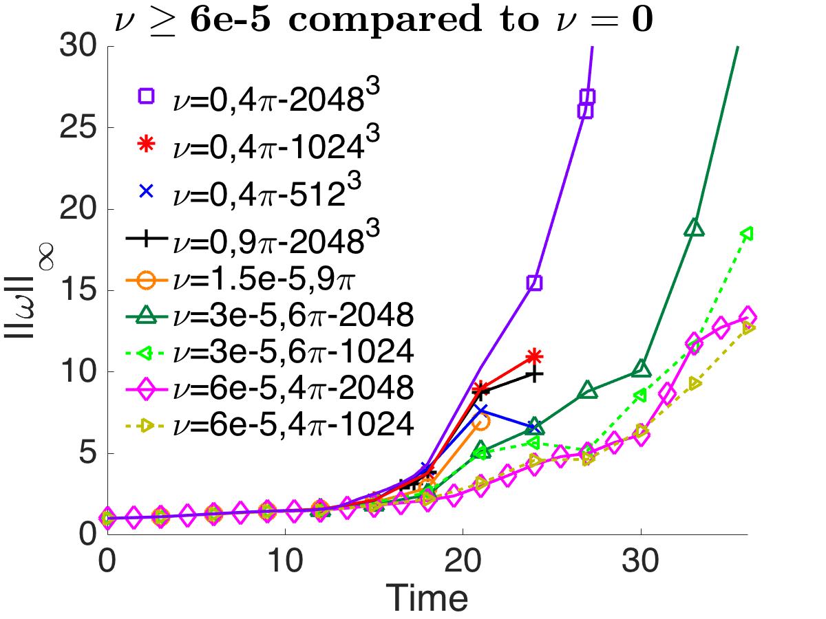
Figure 2: Early time $\|\omega\|_{\infty}$ for Euler and small $\nu$ Navier-Stokes calculations. The Navier-Stokes $\|\omega\|_{\infty}$ are used for resolution checks in section 2.1 and all of the $\|\omega\|_{\infty}$ curves are used in section 7 to address possible mathematical constraints upon the new scaling behaviour. There are four Navier-Stokes cases using two viscosities, $\nu=6.25$e-5 with $\ell=4\pi$ and $\nu=3.125$e-5 with $\ell=6\pi$, with each calculated on both $1024^{3}$ and $2048^{3}$ meshes. There are three Euler calculations in a $\ell=4\pi$ domain at resolutions of $512^{3}$, $1024^{3}$ and $2048^{3}$ and one $\ell=9\pi$, $2048^{3}$ Euler calculation.

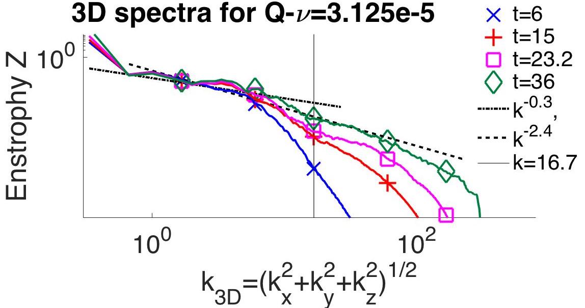
Figure 3: For provide resolution checks, Navier-Stokes enstrophy spectra for the $\nu=3.125$e-5, $2048^{3}$ calculation at $t=6$, 15, 23.2 and 36. There are two spectral regimes. A growing, nearly flat lower-wavenumber $k^{-0.3}$ regime and higher-wavenumber $Z(k)\sim k^{-2.4}$ (or energy $E(k)\sim k^{-4.4}$).

Two approaches have been used to determine the limits in time and decreasing viscosity over which the diagnostics can be believed for a given resolution and domain size. One approach, shown in figure 2, is to compare the evolution of $\|\omega\|_{\infty}$ for different resolutions and viscosities The other approach is to follow the evolution of enstrophy spectra such as those from the $\nu=3.125$e-5 case in figure 3. The Navier-Stokes comparisons will be discussed next. The discussion of the Euler calculations and the comparisons between Euler and Navier-Stokes are in section 7.

For Navier-Stokes comparisons, figure 2 uses two viscosities, $\nu=3.125$e-5 and $\nu=6.25$e-5 with two resolutions for each, $1024^{3}$ and $2048^{3}$. Of these four calculations, even though the $\nu=6.25$e-5, $\ell=4\pi$ $2048^{3}$ calculation is the only one judged to be fully resolved in terms of $\|\omega\|_{\infty}$ and spectra, all except the $\nu=3.125$e-5, $\ell=6\pi$, $1024^{3}$ case provide reliable results for the enstrophy $Z$.

The $\nu=3.125$e-5 three-dimensional enstrophy spectra shown in figure 3 can be used to assess whether calculations are adequately resolved as follows. First note that for this $\nu=3.125$e-5 case there are exponential tails to the spectra up to $t=24$, a signature that they are fully resolved. For the $\nu=6.25$e-5 $\ell=4\pi$ cases (not shown), the $2048^{3}$ spectra have exponential tails for all times, but for the $1024^{3}$ case, there are spectral tails only up to $t=24$, similar to those in figure 3. Due to this, between $t=31$ and $t=36$, the $\|\omega\|_{\infty}$ for the $1024^{3}$ case are below those for the $2048^{3}$ case in figure 2. Furthermore, at no time are there any discernible differences in the enstrophies, $Z$ for the $\nu=6.25$e-5, $1024^{3}$ and $2048^{3}$ cases.

Why doesn’t the drop in $\|\omega\|_{\infty}$ due to inadequate resolution affect the growth of the enstrophy $Z$ for the $\nu=6.25$e-5, $1024^{3}$ and $3.125$e-5, $2048^{3}$ calculations? This can be understood by noting how the growing enstrophy-containing, lower-wavenumber, approximately $Z(k)\sim k^{-0.3}$ regime gradually expands into the $Z(k)\sim k^{-2.4}$ power law regime. A regime whose magnitude increases, but slope does not, as it extends to the highest wavenumbers, as indicated for $t=36$. This $k^{-2.4}$ regime shields the $k^{-0.3}$ enstrophy-containing wavenumber regime from the high-wavenumber cutoff and small-scale errors. This effect also applies to the early-time ($t\leq 24$) very small $\nu$ enstrophies plotted in figure 12 and discussed in section 7.

Based upon these observations, because the $\nu=3.125$e-5, $\ell=6\pi$, $2048^{3}$ resolution case is mildly underresolved for a brief period after $t\approx 30$, the $\nu<3.125$e-5 cases are not among the primary rescaled enstrophy curves in figures 4 and 5. The exception in each figure is one gray, dashed $\nu=2$e-6 curve, that shows how robust the small $\nu$ scaling of $\sqrt{\nu}Z(t)$ is for small $\nu$ up to $t=t_{x}\approx 40$ and connects the early time, very small viscosity cases given in figure 12 to the higher viscosity cases.

2.2 Trefoil length and time scales

To compare these simulations to the experiments in section 6.and earlier simulations, the important length and time scales are needed. The three length scales in the initial condition (17) are the trefoil’s radius $r_{f}=2$, the separation between its loops $\delta_{a}=2a=1$ and the effective thickness of the filaments $r_{e}$. Four $r_{e}$ are simulated, designated P, Q, R and S, each halving the area of the trefoil core of the previous set of initial conditions while keeping the circulation $\Gamma$ constant. The focus will be on the Q-trefoils, with results from the S-trefoils used to demonstrate that these results do not depend strongly upon the initial core radii $r_{e}$ for $r_{e}/r_{f}$ that are close to those used by the experiments discussed in section 6.

There are a variety of timescales that can be applied to vortex reconnection events, either nonlinear, viscous or maybe a combination of the two. The results for scaled enstrophy $\sqrt{\nu}Z$ growth in figure 4 and helicity evolution in figure 11 will show that the correct dynamical timescale should not depend upon either the domain size $\ell$ or the core thickness $r_{e}$. A traditional large-eddy turnover time $t_{L}$ can be determined using the mean velocity scale of the energy and the size of the structure $r_{f}$

$$t_{L}=r_{f}/U,~{}{\rm where}\quad U=\sqrt{2E_{0}}\,.$$ (20)

Table 1 shows that $E_{0}$ is a function of domain $\ell$ and the thickness of the cores $r_{e}$, so $t_{L}$ depends upon $\ell$, $r_{e}$ and $r_{f}$ and is not an appropriate nonlinear timescale.

A better timescale for these simulations is to use the strength of the nonlinear convective motion, given by the circulation $\Gamma$ and the size of the structure. Using $\Gamma$ and either $r_{f}$ or $a$ gives the following two nonlinear timescales for the trefoils:

$$t_{f}=r_{f}^{2}/\Gamma=8\quad{\rm and}\quad t_{a}=\delta_{a}^{2}/\Gamma=t_{f}/4=2\,.$$ (21)

$t_{f}$ will be used for comparisons with the experiments and $t_{a}$, based upon the separation of the loops, will be used for comparisons between the trefoil and anti-parallel reconnection in section 4.

Furthermore, using $\Gamma$ and $r_{f}$ gives the characteristic velocity scale of

$$u_{f}=\Gamma/r_{f}=0.505/2=0.25\,.$$ (22)

The initial peak velocity and downward ($-z$) translation velocity of the position of $\|\omega\|_{\infty}$ are $\|u\|_{\infty}\approx u_{z}(\|\omega\|_{\infty})\approx-0.25=-u_{f}$. The velocities $\|u\|_{\infty}$ and $|u_{z}(\|\omega\|_{\infty})$ decrease slightly until $t=10$, then increase. The change in peak velocity behaviour at $t=10$ could be a precursor to the $(\sqrt{\nu}Z(t))^{-1/2}$ collapse for the trefoils discussed in section 3.2.

However, if the trefoils’ nonlinear timescale is $t_{f}=8$, the most important physical time is $t_{x}\approx 40=5t_{f}=20t_{a}$, which is when the $\sqrt{\nu}Z(t)$ approximately meet in figure 4 and when the first reconnection ends, as discussed in section 5. Resolving these incongruous timescales is one of the goals of this paper.

3 Scaling during first reconnection at $t_{x}$

The first indications for a new type of $\sqrt{\nu}Z(t)$ scaling for trefoil reconnection came from the $\nu$-independent crossing of $\sqrt{\nu}Z(t)$ at $t=t_{x}\approx 40$ for the first five Q-trefoils in figure 4a. The two vertical lines show $t_{x}$, the time for the $\sqrt{\nu}Z(t)$ convergence and $t_{\epsilon}\approx 2t_{x}$, a later, more approximate time when a common value for the energy dissipation rates $\epsilon=\nu Z$ is attained. Frame 4b highlights this second convergence by plotting $\epsilon$ for three viscosities.

The first four cases using a $(4\pi)^{3}$ domain cover $\nu=5$e-4 to $\nu=6.25$e-5 while the green $\nu=3.125$e-5 calculation uses a $(6\pi)^{3}$ domain. There are two additional $\sqrt{\nu}Z(t)$ evolution curves in the main frame. The gray-dashed $\nu=$2e-6 curve and the brown-marked $\nu=$3.125e-5 curve that comes from a $\nu=3.125$e-5 calculation using a smaller $\ell^{3}=(4\pi)^{3}$, domain than the $(6\pi)^{3}$ calculation whose $\sqrt{\nu}Z(t)$ crosses with the other $\nu<$3.125e-5 curves at $t_{x}=40$.

This dependence of $\sqrt{\nu}Z(t)$ on $\ell$ is general. That is, when $\nu=$6.25e-5 and a $(3\pi)^{3}$ domain was used, $\sqrt{\nu}Z(t_{x})<0.14$, but with the $(4\pi)^{3}$ domain it does cross the others in figure 4a with $\sqrt{\nu}Z(t_{x})=0.14$. As the viscosity is decreased further, to $\nu\leq 1.5625$e-5, the $\sqrt{\nu}Z(t_{x})$ converge at $t_{x}\approx 40$ only if $\ell$ is increased still further. First to $\ell=9\pi$ and then to $\ell=12\pi$, as in the $\nu=2$e-6 gray-dashed curve that is included to demonstrate the robustness of the of the convergence of $\sqrt{\nu}Z(t)$ at $t=t_{x}\approx t_{x}\approx 40$ even when the viscosity has changed by a factor of at least 256 and the calculation is clearly under-resolved in terms of $\|\omega\|_{\infty}$.

3.1 Mathematics underlying increasing $\ell$

Why must the domain be increased as the viscosity is decreased? A plausible answer comes from considering this question: As $\nu$ decreases, could there be critical viscosities $\nu_{s}$ such that for $\nu<\nu_{s}$, the Navier-Stokes norms are bounded?

This question was considered by Constantin (1986) who showed that if in a fixed periodic domain the Euler solution for a particular initial condition is regular (non-singular) up to a time $T$, then for $\nu<\nu_{s}$, a critical viscosity, the higher-order $s>5/2$ Sobolev norms (7) for the differences between the Navier-Stokes $u(t)$ and Euler $v(t)$ solutions are bounded as follows:

$$\sup_{t\in[0,T]}\|{u(t)-v(t)}\|_{H^{s}_{\ell}}\leqq\nu_{s}\gamma_{s}\,,$$ (23)

where the $\gamma_{s}$ are viscosity independent functions of the regular Euler norms and the $\nu_{s}$ depend upon $\ell$ as follows

$$\nu_{s}(\ell)\sim\ell^{-2s+5}\left\{\mbox{functions of Euler time integral}\right\}\rightarrow 0~{}~{}{\rm as}~{}~{}\ell\rightarrow\infty~{}~{}{\rm for}~{}~{}s>5/2\,.$$ (24)

Once these bounds on the higher-order $\|{u}\|_{\dot{H}^{s}_{\ell}}$ norms are established, then a chain of $\ell$ dependent Sobolev space embedding inequalities can show that these norms would in turn bound $\|{\omega}\|_{L^{\infty}}$ from above. That the early time Navier-Stokes $\|{\omega}\|_{L^{\infty}}$ are bounded at early times by the non-singular Euler $\|{\omega}\|_{L^{\infty}}$ is shown in figure 2. From this, the standard Hölder inequality will bound the volume-integrated enstrophy $Z\leq\ell^{3}\|{\omega}\|_{\infty}^{2}$ (12), with a very strong $\ell$-dependent pre-factor. $\square$

$\bullet$ Note that despite the Constantin (1986) restriction on the growth of enstrophy $Z$ as $\nu\rightarrow 0$ for fixed $\ell$, because the $\nu_{s}(\ell)$ depend inversely upon the domain size $\ell$, those restrictions can be relaxed simply by making the domain larger. Figures 4 and 5 show how that allows $\sqrt{\nu}Z(t)$ to collapse onto a self-similar curve as $\nu$ decreases. Given this, the following questions are to be addressed in the following sections:

1. How will simulations with smaller viscosities, in larger domains, behave?

   • Small viscosities will be considered in section 7.

2. What type of physical space mechanism could connect the distant periodic boundaries to the enstrophy generation mechanisms within the original trefoil?

   • A physical space mechanism will be considered with respect to the negative helicity isosurface in figure 10 at $t=45$ and in section 6.

3. Why does the growth of $\sqrt{\nu}Z$ have self-similar scaling instead of the dissipation $\epsilon=\nu Z$?

   • This and whether there could be any type of self-similar collapse in the period $0\lesssim t\leq t_{x}$ are now discussed in section 3.2.

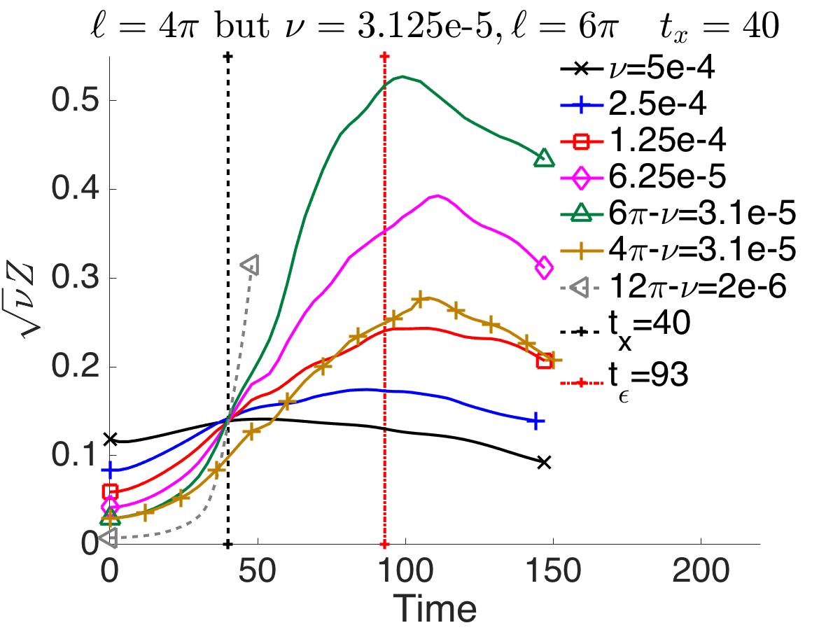
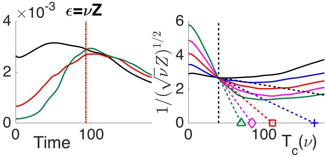
Figure 4: a: Time evolution of the scaled enstrophy $\sqrt{\nu}Z$. Note that all the curves, except the brown-+ curve, cross at $\sqrt{\nu}Z(t_{x})=0.14$, $t_{x}\approx 40$. The time $t_{x}=40$ is identified as the end of the first reconnection using graphics that includes figure 10 at $t=45$. The brown-+ curve is from a $\nu=3.125$e-5, $(4\pi)^{3}$ calculation, the same domain as the other viscous cases, but $\sqrt{\nu}Z(t=40)\neq 0.14$. Unlike the $\nu=3.125$e-5 green curve which was run in a $(6\pi)^{3}$ domain. The importance of increasing the size of the domain as the viscosity is decreased comes from the mathematical analysis of Constantin (1986) expressed by (24). The red line at $t_{\epsilon}=93$ is when plots of the dissipation rate $\epsilon=\nu Z$ cross. b: $\epsilon=\nu Z$ for three cases, $\nu=5$e-4, 1.25e-4 and 3.125e-5 that show it crossing at $t_{\epsilon}=93$. c: This shows the transitional plot that determines $T_{c}(\nu)$ for the time scaling in figure 5. $T_{c}(\nu)$ is found by plotting $B_{\nu}(t)=(\sqrt{\nu}Z(t))^{-1/2}$ (25), then drawing lines between $t_{\Gamma}=15$ and $t_{x}$ that are extended to $B_{\nu}(t)=0$, giving us the effective singular times $T_{c}(\nu)$ indicated by the symbols in the upper caption. The $\Delta t(\nu)=T_{c}(\nu)-t_{x}$ are used in the (27) scaling of $B_{\nu}(t)$ that is plotted in figure 5.

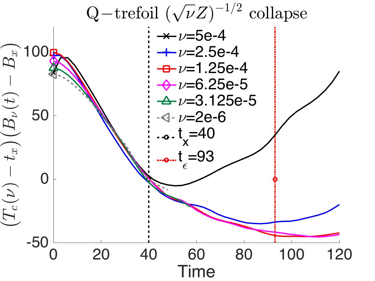
Figure 5: Evolution of the inverse, scaled enstrophy using (27) with $B_{\nu}(t)=(\sqrt{\nu}Z(t))^{-1/2}$ (26) and $B_{x}=B_{\nu}(t_{x})$. The left symbols are $t=0$ for each $\nu$ calculation. This collapse to early times indicates that the dynamics leading to the crossing of $\sqrt{\nu}Z(t)$ at $t=t_{x}$ begins relatively early and even extends to $t>t_{x}$. The collapse begins at $t_{\Gamma}=15$, an early time relative to $t_{x}=40$, begins as soon as negative helicity appears in the vicinity of the closest approach of the two loops as discussed in section 6.2. That viscosity plays a role almost immediately as discussed in section 7 using figure 12.

3.2 Self-similar scaling in time

After searching for, and not finding, any clear indications that the energy dissipation rate $\epsilon=\nu Z$ might have a direct role in the reconnection process, the $\sqrt{\nu}Z(t)$ diagnostic was explored based upon the anti-parallel circulation exchange results illustrated in figure 8 and discussed in section 4. Both the circulation exchange rate for anti-parallel reconnection $\epsilon_{\Gamma}$ (29) and the $\sqrt{\nu}Z(t)$ diagnostic have the earmarks of Leray (1934) scaling, as discussed in section 4.1.

While seeing the crossing of all the $\sqrt{\nu}Z(t)$ in figure 4a at a $\nu$-independent time $t_{x}$ is tantalising, the observation would be more significant if it could be associated with a self-similar collapse. The path to finding a self-similar collapse for $t\leq t_{x}$ is in figure 4c which, in addition to showing $t\leq t_{x}$ linearly decreasing

$$B_{\nu}(t)=\bigl{(}\sqrt{\nu}Z(t)\bigr{)}^{-1/2}=\bigl{(}\nu^{1/4}\|{\omega(t)}\|_{L^{2}(\mathbb{T}_{\ell}^{3})}\bigr{)}^{-1/2}\,,$$ (25)

shows linear extrapolations of $B_{\nu}(t)$ from the earliest time that $B_{\nu}(t)$ is linear, designated $t_{\Gamma}\approx 15$ for each Q-trefoil, through $t_{x}$ to the linearly extrapolated critical times $T_{c}(\nu)$ defined by

$$T_{c}(\nu)=\bigl{(}t_{x}-t_{\Gamma}B_{x}/B_{\nu}(t_{\Gamma})\bigr{)}/\left(1-B_{x}/B_{\nu}(t_{\Gamma})\right)$$ (26)

where $B_{x}=B_{\nu}(t_{x})=\bigl{(}\sqrt{\nu}Z(t_{x})\bigr{)}^{-1/2}$

Physically, for the Q-trefoils $t_{\Gamma}$ is roughly when negative $h<0$ helicity density first appears and for the anti-parallel cases in section 4, $t_{\Gamma}$ is when an exchange of the circulation $\Gamma$ between the vortices begins and is why this early time is designated as $t_{\Gamma}$.

Using these $T_{c}(\nu)$, $t_{x}$ and $B_{x}$, figure 5 plots the following rescaled enstrophy

$$(T_{c}(\nu)-t_{x})\bigl{(}B_{\nu}(t)-B_{x}\bigr{)}=(T_{c}(\nu)-t_{x})\left(\frac{1}{(\sqrt{\nu}Z(t))^{1/2}}-B_{x}\right)\,.$$ (27)

For the trefoils, the collapse to this form develops at early times compared to $t_{x}$, even though the rescaling was chosen empirically and does not obey the time scaling implied by the Leray analysis, as discussed in section 4.1. A side benefit of the collapse to early times given by (27) is that this justifies making a connection between the very small viscosity, early time analysis of section 7 to the crossing of the $\sqrt{\nu}Z(t)$ at $t=t_{x}=40$ in figure 4a.

4 Anti-parallel reconnection: Circulation exchange and $\sqrt{\nu}Z$ collapse

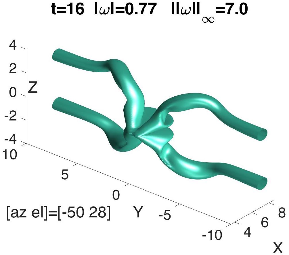
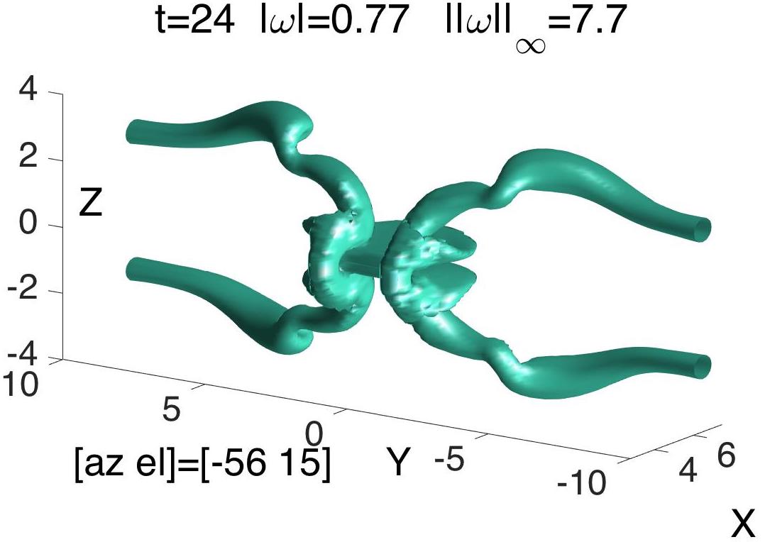
Figure 6: Anti-parallel vortex isosurfaces at $t=16\approx t_{\Gamma}=16.5$ and $t=24\approx t_{x}$. Reconnection is just beginning at $t=16$ and the structure is nearly identical to the final stage in anti-parallel Euler calculations (Kerr, 2013b). The period $t_{\Gamma}=16.5\leq t\leq t_{x}\approx 25.5$ covers the first reconnection, with the $t=24$ frame showing how the heads reconnect across the $z=0$ plane to form vertical $\omega_{z}$ bridges with gaps in the original horizontal $\omega_{y}$, whose remnants on the $y=0$ symmetry plane are concentrated in two vortex sheets.

The second set of calculations showing $(\sqrt{\nu}Z(t))^{-1/2}$ scaling are new anti-parallel calculations using the same initial state as in Kerr (2013a), but higher Reynolds numbers, shorter $y$-domains and larger $z$-domains. As then, the circulation of the initial $y$-vorticity is $\Gamma_{y}\approx 5$ and the separation of the vortices is $\delta_{a}=2a=4$ with $t_{a}=3.2$. Figure 6 shows the full periodic vortex structures as the first reconnection begins at $t=16$ and ends at $24$.

Two advantages of the anti-parallel configuration for studying the beginning of reconnection are that more resolution can be applied to the reconnection zone and how the components of vorticity are attached to one another can be easily identified. The disadvantages are that due to symmetries the global helicity is identically zero and the initial integral norms increase as the domain is increased, making comparisons to the mathematics problematic.

Between the beginning and end of reconnection in figure 6, figure 8 shows collapse using (27) of $B_{\nu}(t)$ (25) similar to that shown for the trefoil in figure 5. The anti-parallel domain size, in these cases just in $z$, must also be increased for the smaller viscosities to see the $B_{\nu}(t)$ collapse. What the anti-parallel cases can do in figure 8, that the trefoil cases have not yet done, is show how the $\sqrt{\nu}Z(t)$ scaling begins. This is with a spurt of $\nu$-independent circulation exchange between the reconnecting vortices. The properties plotted are the $y=0$ and $z=0$ symmetry-plane circulations, $\Gamma_{y}(t)$ and $\Gamma_{z}(t)$, defined as:

$$\begin{array}[]{rl}\vskip 6.0pt plus 2.0pt minus 2.0pt\Gamma_{y}(t)=\int_{y=0}\omega_{y}dx\,dz,{}&\mbox{the integral of}~{}\omega_{y}~{}\mbox{on the $x\!-\!z$ perturbation plane.}\\ \Gamma_{z}(t)=\int_{z=0}\omega_{z}dx\,dy,{}&\mbox{the integral of}~{}\omega_{z}~{}\mbox{on a $x-y$ dividing, symmetry plane,}\end{array}$$ (28)

and $\epsilon_{\Gamma}(t)$, the viscous exchange of circulation between the symmetry plane. This is defined as this integral along the $y=z=0$ $x$-line where the two symmetry planes meet:

$$\epsilon_{\Gamma}(t)=\nu\int dx\left(\frac{\partial^{2}}{\partial_{y}^{2}}+\frac{\partial^{2}}{\partial_{z}^{2}}\right)u_{x}(t)=\frac{d\Gamma_{y}}{dt}(t)=-\frac{d\Gamma_{z}}{dt}(t)\,.$$ (29)

The line integrals $x\in{\cal C}_{j}$, $j=y$ or $z$, (5) for $\Gamma_{y}(t)$ and $\Gamma_{z}(t)$ follow the perimeters of the two symmetry planes.

• Note that because $d\Gamma_{y}/dt=-d\Gamma_{z}/dt=\epsilon_{\Gamma}$ exactly, the sum $\Gamma_{y}(t)+\Gamma_{z}(t)=\Gamma_{y}(t=0)$ is constant during this process.

What figure 8 shows is that at a $\nu$-independent time of $t_{\Gamma}\approx 16.5$, the depletion of the original circulations and the generation of reconnected circulations all cross as the exchange rates $\epsilon_{\Gamma}$ collapse onto a common curve for the three smallest viscosities.

Two immediate effects of this finite circulation exchange are shown by the $t=16$ vorticity isosurfaces of figure 6. The formation of significant isosurface of nearly vertical reconnected $\omega_{z}$ and the collapse of the remaining $\omega_{y}$ from the initial state into a horizontal vortex sheet. The $t=24$ frame shows how this first reconnection ends, with almost all of circulation transferred into the new vortices and the formation of twist and helicity along the vortices.

How are the structures at these two times related to the times covered by the linearly decreasing self-similar collapse (27) in figure 8? The first time, designated $t_{\Gamma}=16$ is when both the exchange of circulation $\Gamma$ during reconnection and the self-similar collapse begin, and the second time, $t=24\approx t_{x}=25$ is when both the reconnection and self-similar collapse end.

The evidence is that by using $t_{\Gamma}=15$ and $t_{x}=40$ for the Q-trefoil that $t_{\Gamma}\leq t\leq t_{x}$ is also the period for self-similar $B_{\nu}(t)$ collapse, as discussed in section 3.2, and for the period of first reconnection, to be discussed in section 5.

What are $t_{\Gamma}$ and $t_{x}$ for the Q-trefoil and anti-parallel in terms of their respective $t_{a}$, the nonlinear timescales (21) based upon the separations of their reconnecting strands? For the anti-parallel cases, one can choose $t_{\Gamma}=16.5\approx 5t_{a}$ to represent the maximum of the circulation exchange due to reconnection. For the Q-trefoils, $t_{\Gamma}=15=7.5t_{a}$, based upon when linearly decreasing $B_{\nu}(t)$ (25) appears in figure 5 and the first appearance of negative helicity, as discussed in section 6.2. In terms of $t_{a}$, the trefoil’s helicity might be delaying the start of reconnection.

For $t_{x}$ determined by either when their respective $B_{\nu}(t)$ (25) cross or when gaps appear in their respective vorticity isosurfaces, for the anti-parallel cases $t_{x}\approx 25=7.8t_{a}$ and for the Q-trefoil, $t_{x}=40=20t_{a}$ This shows that the helicity slows the trefoil reconnection process considerably once it has started and it was the long duration of this phase that first indicated the possibility of the new scaling about $t=t_{x}$ in a way that the anti-parallel calculations did not.

Figure 7: Anti-parallel circulation exchange. Between $t=14$ and 18 there is a small, but finite, viscous exchange of circulation between the two symmetry planes. The rate of change $\epsilon_{\Gamma}$ can be predicted exactly by a line integral (29) where the $y=0$ and $z=0$ symmetry planes meet and is plotted for each case. The time of the maximum of this viscous exchange retreats back towards $t=16$.

Figure 8: Evolution of the inverse, scaled enstrophy for the new anti-parallel calculations using (27) with $B_{\nu}(t)=(\sqrt{\nu}Z(t))^{-1/2}$ (26) and $B_{x}=B_{\nu}(t_{x})$. This scaling regime begins with the brief self-similar exchange of circulation in figure 8 at $t_{\Gamma}\lesssim 16.5$. The three-dimensional structure of the reconnecting vortices at later times is given in Kerr (2013a).

4.1 Leray similarity and extensions.

For the line integral that determines $\epsilon_{\Gamma}(t)$ (29) to remain finite as the viscosity decreases, the second derivative of the velocity terms $(\partial_{y}^{2}+\partial_{z}^{2})u_{x}$ must grow in a singular manner. How it grows can be understood in terms of the Necas et al. (1996) extension of the original similarity proposal of Leray (1934).

Given the Navier-Stokes equation (1), Leray (1934) proposed the following scaling for solutions of the Navier-Stokes equation:

$$\mbox{\boldmath$u$}(\mbox{\boldmath$x$},t)=\frac{\Gamma_{L}}{\delta_{\nu}(t)}\mbox{\boldmath$f$}(\mbox{\boldmath$y$})=\frac{1}{\delta_{\nu}(t)}\mbox{\boldmath$\Gamma$}(\mbox{\boldmath$y$})\quad{\rm or}\quad\mbox{\boldmath$u$}(\mbox{\boldmath$x$},t)=U_{\nu}(t)\mbox{\boldmath$f$}(\mbox{\boldmath$y$})$$ (30)

where $\delta_{\nu}(t)\sim\sqrt{2a_{L}(T-t)}$ is a collapsing length scale, $\mbox{\boldmath$y$}=\mbox{\boldmath$x$}/\delta_{\nu}(t)$, $U_{\nu}(t)=\Gamma_{L}/\delta_{\nu}(t)\sim(\Gamma_{L}/\sqrt{2a_{L}})(T-t)^{-1/2}$ and $\mbox{\boldmath$\Gamma$}(t)=\Gamma_{L}\mbox{\boldmath$f$}(\mbox{\boldmath$y$})$ sets the spatial structure. The scalars $a_{L}$ and $\Gamma_{L}$ have the same units as the viscosity and circulation. Inserting (30) in (1) one gets

$$\begin{array}[]{r}-\nu\Delta\mbox{\boldmath$\Gamma$}+a_{L}\mbox{\boldmath$\Gamma$}+a_{L}(\mbox{\boldmath$y$}\nabla\mbox{\boldmath$\Gamma$})+(\mbox{\boldmath$\Gamma$}\mbox{\boldmath$\cdot$}\nabla)\mbox{\boldmath$\Gamma$}+\nabla P=0\\ \nabla\mbox{\boldmath$\cdot$}\mbox{\boldmath$\Gamma$}=0\end{array}\Bigr{\}}\quad{\rm in}~{}\mathbb{R}^{3}$$ (31)

The similarity predictions of some aspects the new $\sqrt{\nu}Z(t)$ regime and whether these are observed, even if only briefly, are now considered. The predictions are obtained by multiplying $U_{\nu}(t)=\Gamma_{L}/\delta_{\nu}(t)$ and $\delta_{\nu}(t)$ in the appropriate dimensional combinations. To begin, the similarity Leray prediction for $\|{\omega}\|_{\infty}$ is

$$\|{\omega}\|_{\infty}\sim U_{\nu}(t)\nabla\cdot(\mbox{\boldmath$x$}/\delta_{\nu})f’\sim U_{\nu}(t)/\delta_{\nu}(t)=\frac{\Gamma_{L}}{\nu(T_{c}-t)}\,.$$ (32)

This is not observed except for $t<20$ when the calculations are nearly Euler. That is, Navier-Stokes $1/\|{\omega}\|_{\infty}$ is briefly linear in time, but figure 2 shows that the Navier-Stokes $\|{\omega}\|_{\infty}$ are all bounded by the non-singular growth of the Euler $\|{\omega}\|_{\infty}$ for $t>20$. This is discussed further in section 7.

What is the Leray similarity prediction for the cubic velocity norm $L^{(3)}_{\ell}$ (8)? Using (30) one gets

$$L^{(3)}=L^{(3)}_{\ell=\infty}=\|{u}\|_{L^{3}(\mathbb{R}^{3})}\sim\left(U_{\nu}^{3}(t)\delta_{\nu}^{3}(t)\right)^{1/3}\sim{\cal O}(1)\,.$$ (33)

This prediction of constant $L^{(3)}$ is consistent with figure 11c which shows that for two of the trefoil calculations, $L^{(3)}_{\ell}$ is remarkably independent of both time and $\nu$ and decreases less rapidly than the kinetic energy. However, Escauriaza et al. (2003) has shown that bounded $L^{(3)}=\|{u}\|_{L^{3}}$ is the most refined restriction against singularities of the Navier-Stokes equation in a proof by contradiction that uses the scaling in (33), despite the singular assumption in (30).

One way to resolve that apparent contradiction is if one can assume that there are very large effective singular times $T$ such that transient, singular growth could be allowed for some norms, so long as the transients end long before $t=T$ is ever reached. This would be consistent with the very brief Leray growth of $\epsilon_{\Gamma}$ in figure 8. For times after that spurt in circulation exchange, it seems plausible that Leray similarity might set the scale for those norms, but their subsequent time dependence would not obey the Leray similarity prediction. The use of the linearly extrapolated singular times in the self-similar collapse (27) of $B_{\nu}(t)$ in figures 5 and 8 reflects that point of view.

• For those reasons, only the viscosity dependencies will be given for the remaining properties with elements of Leray scaling.

For the circulation exchange in (29), Necas et al. (1996) provides an estimate the second velocity derivatives in (29) where

$$\left(\partial_{x}^{2}+\partial_{y}^{2}\right)u\sim U_{\nu}/\delta_{\nu}^{2}\sim\nu^{-3/2}\,.$$ (34)

Then the Leray scaling for line integral over $\delta_{\nu}(t)$ would be $\epsilon_{\Gamma}\sim(\nu\delta_{\nu})(\nu^{-3/2})\sim{\cal O}(1)$, as observed in figure 8.

Finally, let us consider $\sqrt{\nu}Z$. The $\nu$ dependence of its Leray scaling would be

$$\sqrt{\nu}Z\sim\nu^{1/2}\delta_{\nu}^{3}(U_{\nu}/\delta_{\nu})^{2}\sim{\cal O}(1)\quad{\rm or}\quad Z\sim\nu^{-1/2}\,,$$ (35)

as observed at $t=t_{x}$ in figures 5 and 8.

5 Evolution the trefoil’s topology during reconnection

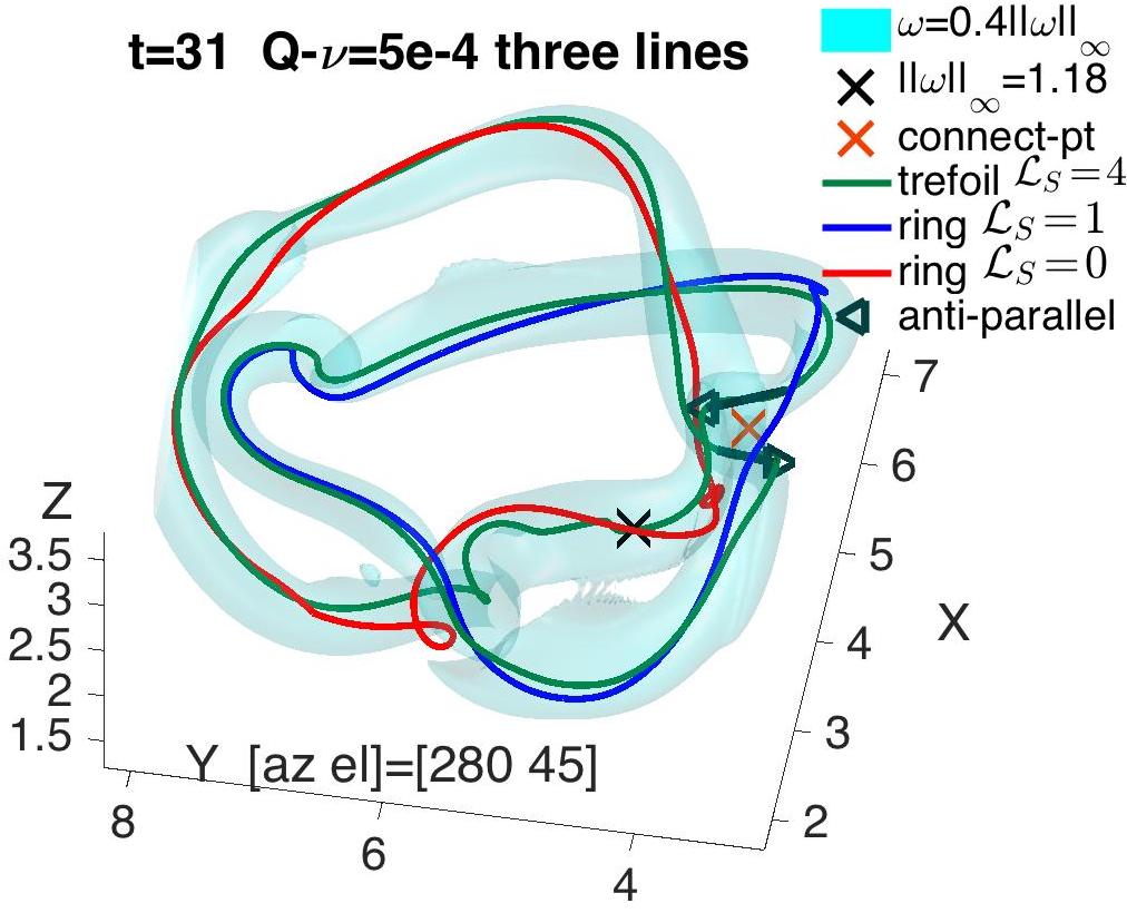
Figure 9: A single vorticity isosurface plus three closed vortex lines at $t=31$, the first time that visible reconnection is observed. The green trajectory follows a trefoil trajectory seeded near $\|{\omega}\|_{\infty}$, indicated by X. The green trajectory’s self-linking is ${\cal L}_{S}=4$, which can be split into $W\!r+T\!w=2.85+1.15=4$ At the closest approach of the trefoil’s two loops, due to an extra twist, the loops are anti-parallel, as indicated by two arrows. Between them is the reconnection zone whose mid-point is shown by the orange cross. The red ${\cal L}_{Sr}=0$ and blue ${\cal L}_{Sb}=1$ linked trajectories were seeded on either side of this point, in the direction perpendicular to the loops’ separation line. Their total linking is ${\cal L}_{t}=2{\cal L}_{rb}+{\cal L}_{Sr}+{\cal L}_{Sb}=2+0+1=3$, the linking of the original trefoil.

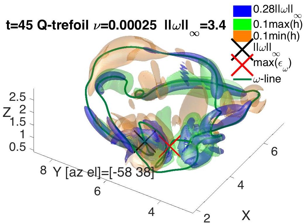
Figure 10: Isosurfaces and one vortex line at $t=45$ just after the first reconnection has ended. Vorticity isosurfaces are in blue and the helicity isosurfaces are at $0.1\max(h)$ in green and $0.1\min(h)$ in yellow, where $\max(h)=0.62$ and $\min(h)=-0.26$. A gap without strong vorticity, but twisted and bent vortices to either side, now covers the reconnection zone to the right of red X. Nonetheless, except in that zone, the vortex line seeded at the point of maximum vorticity at X still has the flavour of the original trefoil as it circumnavigates the centre twice and passes through regions with large vorticity and large helicity of both signs. Green positive helicity overlying twisted blue vorticity dominates to the right of the gap. The region between the black X and red X, to the left of where reconnection began at $t=31$, is now dominated by the negative helicity discussed in section 6.2 along with the additional regions of large negative helicity outside the reconnection zone.

The purpose of this section is to outline the temporal changes to the three-dimensional structure from the beginning of observable reconnection until just after reconnection ends using two times. The position of $\|{\omega}\|_{\infty}$ is the black X and the reconnection zone is indicated by a orange/red X. The definition of the reconnection zone changes with time, but the relative locations of these points with respect to the overall, slowly rotating trefoil structure does not change from where they sat at $t=6$ in figure 1. Figure 9 at $t=31$ was chosen to represent the beginning of reconnection because it was the first time that linked rings, rings whose trajectories originated within the trefoil’s reconnection zone, could be identified. Figure 10 at $t=45$ was chosen to represent the phase just after reconnection has ended because this is the first time that the reconnection has created a clear gap in the the blue vorticity isosurface.

Both figures show one mid-level vorticity isosurface and one green trefoil vortex trajectory with additional diagnostics in each figure highlighting those features that are particularly important for that phase of the evolution. The trefoil trajectories originate at the X, or passes this point, and both circumnavigate the central $z$ axis twice before closing almost exactly upon themselves. The perspectives are tilted so that the overall trefoil structure can be seen with the zone between the red/orange and black X’s in the foreview, a zone that slowly rotates from right to left along with the entire trefoil.

How reconnection begins is shown in figure 9 at $t=31$ using two additional linked single vortex loops in red and blue that were seeded on opposite sides of the orange X, which is the mid-point between the closest approach of the green trefoil’s two loops. Due to an acquired twist in the green trefoil, these segments of the loops are anti-parallel about the orange X, as indicated by the arrows, and define the reconnection zone because this is where anti-parallel, helicity preserving reconnection begins, as discussed further in section 6.2. Due to this twist, by using (15), the total self-linking number (13) of the green trajectory is ${\cal L}_{Sg}=4$. Since the red and blue loops are linked and the blue loop has twist+writhe whose self-linking is ${\cal L}_{Sb}=1$, the total linking number of the red and blue loops is ${\cal L}_{t}={\cal L}_{rb}+{\cal L}_{br}+{\cal L}_{Sb}=3$ using (14) with $\Gamma=1$, equal to the total linking number of the original trefoil. This demonstrates why, if helicity is simply ${\cal H}=\Gamma^{2}{\cal L}$ (14), reconnection by itself need not result in a change in the total helicity (Laing et al., 2015). However, for the continuum Navier-Stokes equations, it is not that simple, as shown by the self-linking of the green trefoil with ${\cal L}_{Sg}=4\neq 3$.

When does the reconnection finish? Figure 10 at $t=45$ tells us that this is before $t=45$ based upon the reconnection zone gap that has formed in the blue vorticity isosurfaces. This is consistent with the reconnection ending at the $t=t_{x}\approx 40$ convergence of $\sqrt{\nu}Z(t)$ in figure 4. This gap is to the right of the position of $\max(\epsilon_{\omega})$ at the red X and unlike in figure 9 at $t=31$, the green trefoil trajectory in figure 10 at $t=45$ goes around this gap, not through it. In addition, the sign and colour of the helicity density $h$ isosurfaces change across the gap. To the right of the gap, positive green helicity surrounds and covers the twisted blue vorticity isosurfaces and to the left of the gap, near the X with $\|{\omega}\|_{\infty}$, negative yellow/orange helicity dominates.

By all of these measures, it is the formation of this gap at $t\gtrsim 40=t_{x}$ that marks the end of the first reconnection and is the most relevant timescale for comparing with the experiments in the next section. Furthermore, the new twists around this gap mark the beginning of a new phase of even stronger enstrophy growth that leads to the development of finite dissipation $\epsilon=\nu Z$ at $t_{\epsilon}\approx 2t_{x}$ in figure 4b. This persists over the finite time interval that follows $t_{\epsilon}$ and would be consistent with the formation of a dissipation anomaly, that is a finite viscosity-independent loss of the total energy in a finite time.

6 Helicity

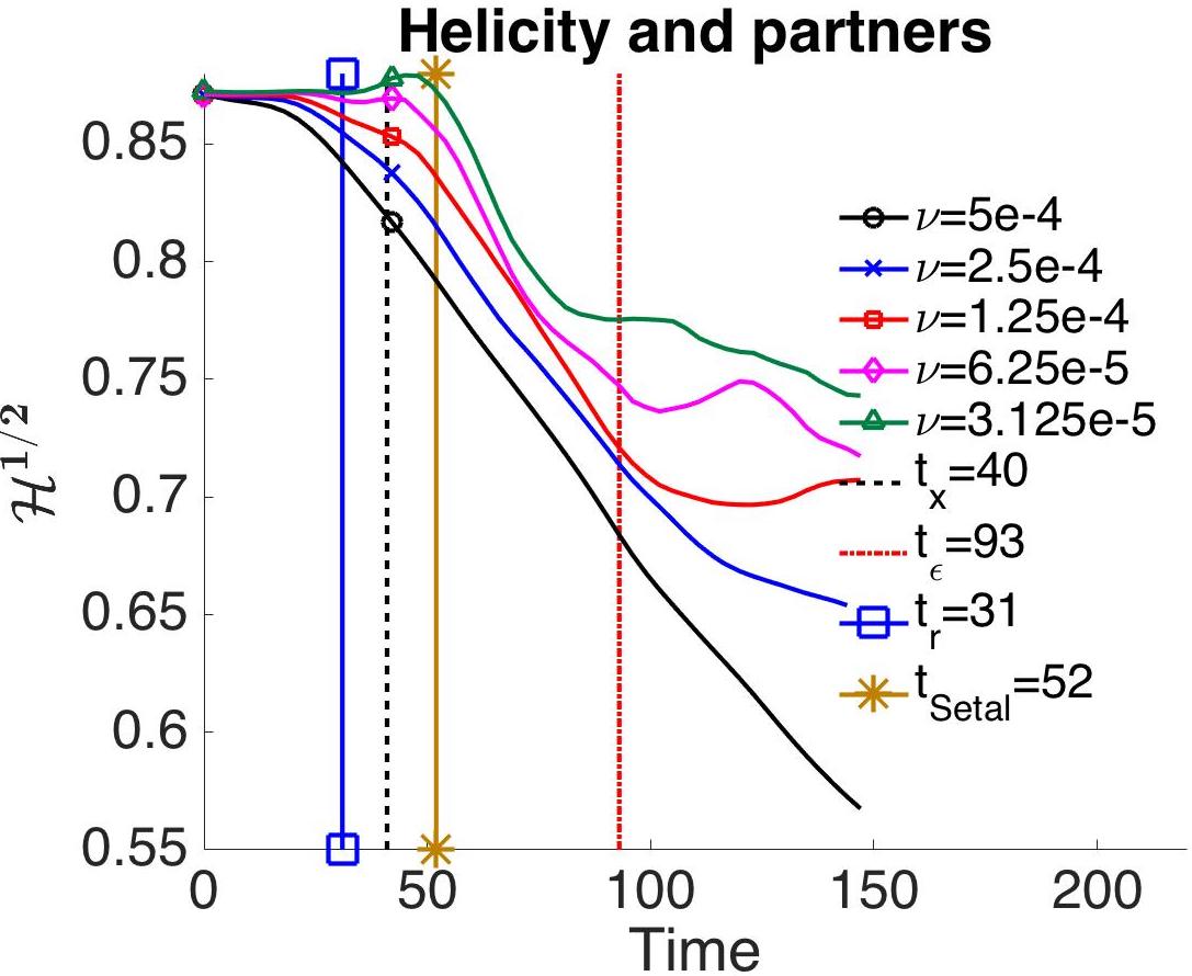
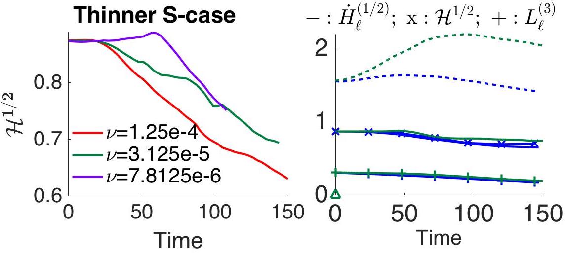
Figure 11: a: Time evolution of the helicity ${\cal H}^{1/2}$ and its partners. In the main frame are 5 viscosities for the Q-trefoils: $\nu=0.0005$ to $\nu=0.00003125$. Also given are important times during the evolution of the trefoil. The blue-$\square$ line is $t=31$, the time when the first signs of reconnection are visible as in figure 9. The dashed line is $t_{x}=40$, the time when all the $\sqrt{\nu}Z$ meet and has been designated the reconnection time. The brown-$\star$ line is $t_{Setal}=52$, roughly the equivalent time to when the Scheeler et al. (2014a) experiment probably ends. The red-dot-dash line is the time $t_{\epsilon}=93$ when the dissipations $\epsilon=\nu Z$ in figure 4 reach a common value. b: ${\cal H}^{1/2}$ for S-trefoils with thinner core radius $r_{e}$ at three viscosities, demonstrating that once the viscosity is small enough that after a long period of helicity preservation, the time when helicity decay begins $t\approx 1.25t_{x}\approx 50$ is independent of the difference in their core thicknesses. c: Comparison of global helicity ${\cal H}$ and two regularity diagnostics. From top to bottom, $\dot{H}^{(1/2)}_{\ell}=\|{u}\|_{\dot{H}^{1/2}(\mathbb{T}_{\ell}^{3})}$ (9) global helicity ${\cal H}^{1/2}$ (4) and $L^{(3)}_{\ell}=\|{u}\|_{L^{3}(\mathbb{T}_{\ell}^{3})}$ (8) for the $\nu=2.5$e-4 and $\nu=3.125$e-5 Q-trefoils. All three diagnostics have been normalised to have the units of circulation and only $\dot{H}^{(1/2)}_{\ell}$ shows a dependence upon the viscosity.

While the focus of this paper has been on comparisons of vorticity norms to mathematical bounds, the inspiration for this study came from the unexpected experimental claim that the centre-line helicity of the vortex knots in Scheeler et al. (2014a) was preserved through reconnection events and for one trefoil case was preserved until the experiment ended.

These experimental trefoil vortices and linked vortex rings were generated and observed by yanking 3D-printed knots, shaped into hydrofoil ribbons, out of a water tank, as described by Kleckner & Irvine (2013). The ribbons were covered with hydrogen bubbles that were shed as the low pressure vortex cores were generated, providing a means for observing those cores. The hydrogen bubble filaments that form within these cores were then used to define the centre-line helicity diagnostics of Scheeler et al. (2014a). Qualitative evidence for when the topology changes was provided by consecutive time-frames when the bubbles on these filaments disperse, then reform.

Many questions have been raised about their unconventional diagnostics, so a set of simulations that could either confirm or explain their results would help. To make those comparisons, common definitions of the nonlinear and reconnection timescales, $t_{f}$ (21) and $t_{x}$ are needed, where figure 4 defines $t_{x}$ for the simulations. Ideally, the definitions of both $t_{f}$ and $t_{x}$ should be related to some aspect of the trajectories of the observed vortex lines because this is the only diagnostic provided by the experiments. What properties might the experimental trajectories and the vortex lines of the simulations share? Due to the intricate and under-resolved structures that form during reconnection in both the experiments and simulations, looking for common properties at the reconnection time has been difficult.

6.1 Experimental reconnection and helicity depletion timescales

There are two routes for estimating the experimental timescales.

• An estimate for the nonlinear timescale $t_{f}$ (21) can be made using the estimated circulations $\Gamma$ of the shed vortices and the radii of the knots $r_{f}$ (17). While the radii can easily be determined for both the experiments and these simulations, the circulations $\Gamma$ given for the experiments were not measured, but estimated based upon the flat plate estimate for how flow over the hydrofoil generates $\Gamma$. This approximation neglects the camber of the trefoil ribbon. Therefore, only the order of magnitudes of the scaled times $t/t_{f}$ between the simulations and the experiments can be compared.

• A visual timescale for $t_{x}$ can be determined from the experimental reconnection figures by first identifying the first clear, visible gap in the trefoil structure. Since this is after the reconnection ends, a better estimate of the reconnection times $t_{x}$ for the experiments is the first frame before the clear gap with evidence that the topology is changing. That is consecutive frames when the bubble lines disperse, then reform.

For these simulations, the clear gap in figure 10 at $t=45$ is consistent with the reconnection being after the inferred end of reconnection at $t_{x}\approx 40$. For the largest trefoil from Kleckner & Irvine (2013), with a camber correction applied to the flat-plate method for estimating the circulation $\Gamma$, the two methods for estimating $t_{x}$ give consistent values, with a reconnection time of $t_{x}\approx 350$ms. Comparisons between Q-trefoil figures at $t=36$, 40 and 45 and the $t=300$, 350 and 400 figures from Kleckner & Irvine (2013) show the same stages in their development and are the topic of another paper (Kerr, 2017).

Detailed comparisons with the timescales and movie from Scheeler et al. (2014b) will require detailed graphics using the thinner S-trefoils, for which $t_{x}\approx 40$ and whose ${\cal H}(t)$ for several $\nu$ are given in figure 11b. For now, the visual evidence indicates that its reconnection gap is in the $t=658$ms frame, and looking earlier in the movie, the reconnection would then be at $t_{x}\approx 638$ms. This is the basis for the $t_{\rm Setal}=52$ line in figure 11 indicating when that experiment ends.

The conclusion is that even if figure 11 does not show helicity preservation for all time, it does show that the true helicity ${\cal H}$ (4) can be preserved through, and a bit after, the end of first reconnection at $t=t_{x}\approx 40$. That is, helicity does not decay at all until $t\approx 1.25t_{x}$ and does not decay significantly until $t\gtrsim 1.5t_{x}$, showing consistency with the preservation of the experimental centre-line helicity. It also supports the conclusion that these simulations are representing a physical flow, irrespective of whether any of the $\nu\rightarrow 0$ limits being proposed become accepted.

The similarities in the ${\cal H}$ timescales for the Q and S-trefoils in figure 11 demonstrates that this behaviour is independent of the core thickness $r_{e}$ once $r_{e}$ is sufficiently small. This is also observed for plots of $\sqrt{\nu}Z(t)$ and $(T_{c}(\nu)-t_{x})(B_{\nu}(t)-B(x)$ (27) for several S-trefoils, including the $\sqrt{\nu}Z(t)$ crossing at $t_{x}\approx 40$.

6.2 Negative helicity surfaces

While the experimental bubble filaments might shed light upon the evolution of the global helicity, they cannot tell us what the sign of the helicity along the filaments is or what the helicity is off of the vortex cores. The change in the sign, and colour, of the helicity isosurfaces have already been used to highlight the gap in the reconnection zone in figure 10 at $t=45$ marked by a red X. What are the relationships between the different signs of the helicity and the vorticity isosurfaces outside of the reconnection zone? In particular, how do the $h<0$ zones form and what is their role?

The following is a summary of the evolution of negative helicity using figures 1, 9 and 10 at $t=6$, 31 and 45. Further details, with more figures, are in an additional submitted paper (Kerr, 2017). To relate to later times, three points are marked along the trefoil centreline vortex in figure 1. The vorticity maximum $\|\omega\|_{\infty}$ at the black X plus the red and yellow + points marking the closest approach of the trefoil’s loops and where reconnection will begin.

Noticeable $h<0$ forms very early, growing to the left of the red + point in figure 1 towards the vorticity maximum at the black X. Growth of local negative $h<0$ becomes stronger starting at $t_{\Gamma}=15$ as the linear scaling of $B_{\nu}(t)=(\sqrt{\nu}Z)^{-1/2}$ begins in figure 5. Up until $t=31$, this zone of $h<0$ continues to grow between the now locally anti-parallel loop segments and the position of $\|\omega\|_{\infty}$. The knot on the red trajectory just below the orange-X reconnection point covers this zone of $h<0$. Above the orange X, $h>0$ grows as it envelopes the vorticity isosurfaces. At this stage, the separation of the $h<0$ and $h>0$ zones is largely due to the $\omega$-transport term in (4).

In the next $t>31$ stage, due to locally anti-parallel reconnection, zones of equal magnitude and oppositely signed viscous dissipation form, as predicted by Laing et al. (2015), which leads to the strong $h<0$ yellow zone to the left of the red X, a gap in the vorticity isosurfaces in figure 10 at $t=45$ and a strong green $h>0$ isosurface to the right. This $h<0$ yellow zone is between, but not on, the sharp bends in the blue vorticity isosurfaces. The strongest and most distant $h<0$ yellow isosurface along the top loop of remaining branch of trefoil vortex and is most likely due to the $\omega$-transport term in (4). The $h<0$ zones between this outer loop and the red X can all be associated with velocity advection out of the reconnection zone.

Note that almost all of the green $h>0$ isosurfaces envelope blue vorticity isosurfaces and for the zone to the right of the red X, there are extra twists in the blue vorticity isosurfaces within the green $h>0$ isosurface. These twists show how smaller vorticity scales, enstrophy and $h>0$ can be generated, without increasing the global helicity ${\cal H}$ due to the generation of $h<0$ elsewhere.

Can this simultaneous growth of positive and negative helicity density $h$, an integral of the form $\int|h|d\Omega$, be expressed by one of the global helicity’s two partner norms, $L^{(3)}_{\ell}$ (8) and $H^{(1/2)}_{\ell}$ (9)?

The cubic velocity norm $L^{(3)}_{\ell}$, as discussed in section 4.1, is virtually constant and cannot represent the integral growth of $|h|$. However, $H^{(1/2)}_{\ell}$ does increase, although less rapidly than its upper bound of $\sqrt{2EZ}$, and could represent this growth as $\nu$ decreases as shown in figure 11. Especially when compared with the relatively constant global helicity ${\cal H}^{1/2}$. This suggests that $H^{(1/2)}_{\ell}$ might be the best property to investigate further for what controls (bounds from above) the Navier-Stokes equation, with both applied analysis and numerically.

7 Small or zero viscosity at early times.

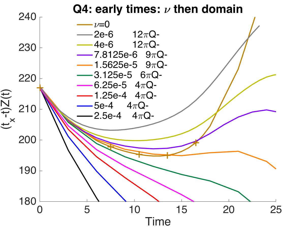
Figure 12: $(t_{x}-t)Z$ at early times when the enstrophies of the Euler and very small $\nu$ calculations are not affected by under-resolution of $\|\omega\|_{\infty}$. The purpose of this figure is to show that as the viscosity continues to decrease, the Navier-Stokes enstrophies can exceed the Euler enstrophy as late as $t=24$. At later times, $\sqrt{\nu}Z$ for the smallest viscosity case, $\nu=2$e-6 in a $(12\pi)^{3}$ domain, joins its continuation in figure 4.

To complement the five $\nu\geq 3.125$e-5 cases in figures 4 and 5, Euler calculations in several different domains and several Navier-Stokes calculations with $\nu\leq 1.5625$e-5 have been run. While all of the $\nu\geq 3.125$e-5 Navier-Stokes calculations are resolved in terms of $Z$ through $t=40$, all of the Euler calculations and the additional $\nu<3.125$e-5 calculations are under-resolved in terms of $\|{\omega}\|_{\infty}$ and spectra for $t>25$. Despite this, these additional calculations are reliable at early times and therefore can address questions that the $\nu\geq 3.125$e-5 calculations cannot.

Questions The first goal for the Euler cases was to determine which of these calculations would be the most representative of later times run in large domains. This included determining whether $\|{\omega}\|_{\infty}$ and $Z$ for fine-resolution calculations would grow in a manner that is consistent with the exponential of exponential Euler growth identified in Kerr (2013b). The second question was whether these Euler norms bound the growth of the equivalent norms for the $\nu\geq 3.125$e-5 Navier-Stokes cases. The Euler norms do bound the norms from the $\nu\geq 3.125$e-5 cases, which is why the additional $2e-6\leq\nu\leq 1.5625$e-5 Navier-Stokes cases were run.

Could the Navier-Stokes $Z$, including the $\nu\leq 1.5625$e-5 cases, be bounded by strong, but finite, Euler enstrophy growth? If so, this would make it less likely that a $\nu\rightarrow 0$ dissipation anomaly could form at $t\approx 2t_{x}$. Or can the enstrophy continue to grow as $\nu$ decreases such that $Z\rightarrow\infty$ as $\nu\rightarrow 0$? First as $Z\sim 1/(\sqrt{\nu}B_{x}^{2})$ at $t=t_{x}$ and then as $Z\sim\epsilon\nu^{-1}$ at $t_{\epsilon}\approx 2t_{x}$ as in figure 4

Euler results Four Euler cases were run, three in a $\ell=\pi$ domain with resolutions of $512^{3}$, $1024^{3}$ and $2048^{3}$, and a fourth case in a $(9\pi)^{3}$ domain using $2048^{3}$ grid points. Figure 2 compares the Euler and Navier-Stokes $\|{\omega}\|_{\infty}$.

While the $\|{\omega}\|_{\infty}$ for the three $\ell=4\pi$ Euler calculations agree up to $t=18$, after $t=18$ the $\|{\omega}\|_{\infty}$ increase as the resolution is improved in a manner consistent with the exponential of exponential growth found for anti-parallel interactions (Kerr, 2013b). The effect of the domain size upon the Euler norms is indicated by the $(9\pi)^{3}$, $2048^{3}$ calculation, with its $\|{\omega}\|_{\infty}$ closely following $\|{\omega}\|_{\infty}$ from the $1024^{3}$ $(4\pi)^{3}$ case, two calculations with roughly the same local resolution. Therefore, using a $(4\pi)^{3}$ is sufficient for determining Euler regularity properties, implying that for $\|{\omega}\|_{\infty}$, the $(4\pi)^{3}$, $2048^{3}$ calculation that is resolved until $t=24$ is the best for comparing to all the Navier-Stokes calculations.

Navier-Stokes comparisons. Next, we want to compare $\|\omega(t)\|_{\infty}$ from the very low viscosity, early time Navier-Stokes calculations to the $(4\pi)^{3}$, $2048^{3}$, Euler values. Up to $t=24$ for the two resolved Navier-Stokes calculations, and even for the $\nu=1.5625$e-5 case up to $t=19$, the $\|\omega(t)\|_{\infty}$ are bounded by the Euler values. This suggests that the superexponential, non-singular growth of $\|\omega\|_{\infty}$ from the $\ell=4\pi$ Euler evolution should bound $\|\omega\|_{\infty}$ for all the viscous cases. Preliminary tests using higher-order $\|{u}\|_{\dot{H}^{s}(\mathbb{T}_{\ell}^{3})}$ show that the $s=2$ and $s=5/2$ Euler norms are also bounding their Navier-Stokes counterparts.

However, the situation is different for the scaled enstrophies $(t_{x}-t)Z$ in figure 12. The Navier-Stokes values do exceed the Euler values over an increasing timespan in a consistent manner as $\nu$ decreases, especially for $\nu\leq 3.125$e-5. The scaling with an extra factor of $(t_{x}-t)$ helps highlight these differences in the Navier-Stokes enstrophy growth at early times. For the lowest viscosity case, $\nu=2$e-6 in a $(12\pi)^{3}$ domain, its $(t_{x}-t)Z$ exceeds the Euler values until $t=21$ and in figures 4 and 5, the grey-dashed curve shows that this eventually connects to the convergence of $\sqrt{\nu}Z$ at $t=t_{x}\approx 40$. $\|{u}\|_{\dot{H}^{s}(\mathbb{T}_{\ell}^{3})}$, for $s=3/2$ and $\nu\geq 1.5625$e-5 shows similar, but much weaker, signs of exceeding its Euler values.

8 Summary and unanswered questions

The trefoil calculations and conclusions presented in this paper have relied upon two types of weaves. One weave generates the perturbed trefoil vortices with a single, dominant initial reconnection.

The second weave shows how restrictions upon the growth of enstrophy can be avoided so that the new scaling regime given in figures 4, 5 and 8 can be identified. A regime that might lead to the formation of a Navier-Stokes dissipation anomaly at later times. That is, $\nu\to 0$ smooth solutions, that generate finite energy dissipation in a finite time without singularities or additional roughness terms,

It was the long, temporal extent of the trefoils’ $\sqrt{\nu}Z(t)$ growth that first indicated the existence of this new scaling regime, with the last step provided by new anti-parallel calculations that provide a mechanism for how the $(\sqrt{\nu}Z(t))^{-1/2}$ scaling regime begins. A useful way to summarise the avoidance steps is to first list them in the order found, then restate them in terms of the forwards-in-time steps of the evolution.

The following steps in the evolution of the trefoil’s enstrophy have been identified,

1. First, as illustrated in figure 4a, it was noticed that for each core radius, all of the $\sqrt{\nu}Z(t)$ crossed at a common time $t_{x}$ so long as the domain size $\ell$ increased appropriately as the viscosity $\nu$ decreased. The $\nu=3.125$e-5 curves in different computational domains show why increasing $\ell$ is needed for maintaining the convergence of $\sqrt{\nu}Z(t)$ at $t=t_{x}$.

2. The large-scale growth of $h<0$, negative helicity, in figure 10 could be providing a mechanism that allows small-scale $h>0$ and enstrophy $Z$ to grow, a mechanism that can be suppressed if the periodic boundaries are too close.

3. Linearly decreasing $(\sqrt{\nu}Z(t))^{-1/2}=B_{\nu}(t)$ (25) for $t\lesssim t_{x}$ was then identified using figure 4c, from which the $T_{c}(\nu)$ needed for the next step were identified.

4. Using these $T_{c}(\nu)$ and $B_{x}$, the $t\leq t_{x}$ linear collapse regimes were identified by determining and plotting $(T_{c}(\nu)-t_{x})\bigl{(}B_{\nu}(t)-B_{x}\bigr{)}$ (27) for both the Q-trefoil and anti-parallel calculations, as shown in figures 5 and 8 respectively.

5. What physical event determines the end of the linear $(\sqrt{\nu}Z(t))^{-1/2}$ collapse? This is identified as the end of the first reconnection using figure 10 and figure 6 for the trefoil and anti-parallel respectively.

6. What determines the beginning of the linear $(\sqrt{\nu}Z(t))^{-1/2}$ collapse? The anti-parallel reconnection calculations identify the beginning of the linear collapse as when the vortices first meet with a brief spurt of circulation exchange that converts a finite fraction of the original $\Gamma_{y}$ into the $\Gamma_{z}$ of the new vortices at $t\approx t_{\Gamma}$.

By reversing these steps the multi-step origins of the new reconnection scaling are these: Inviscid evolution from $t=0$ until the vortices touch, from which a viscous $(\sqrt{\nu}Z(t))^{-1/2}$ scaling regime forms that lasts until the first reconnection ends at $t_{x}$. Figure 10 at $t\!=\!45>t_{x}\!=\!40$ shows that the necessary increase in the enstrophy is associated with local increases in positive helicity and to preserve the global helicity ${\cal H}$, the $h\!>\!0$ increases are balanced by the generation of $h\!<\!0$ at larger scales. The $t\leq t_{x}$ phase is followed a slow decay of the global helicity ${\cal H}(t)$ and further growth in the enstrophy until a there is a finite rate of energy dissipation at $t=t_{\epsilon}$, as shown in figure 4b. As this continues, a dissipation anomaly forms. That is, finite energy dissipation in a finite time is generated.

Further constraints on growth. Let us consider the ways that this progression of increasing $Z$ could be disrupted, and the evidence that it is not.

While increasing the domain skirted around the Constantin (1986) restrictions, since Euler $\|{\omega}\|_{\infty}$ seems to bound the growth of all Navier-Stokes vorticity maxima, could this lead to an upper bound upon the Navier-Stokes enstrophies $Z$? Especially since for Euler both $\|{\omega}\|_{\infty}$ and $Z=\|{\omega}\|_{H^{0}(\mathbb{T}_{\ell})}^{2}=\|{u}\|_{H^{1}(\mathbb{T}_{\ell})}^{2}$ are bounded.

Figure 12 addresses this possibility using early time results from very small viscosity calculations with $\nu\leq 1.5625$e-5. These show that the growth of the Navier-Stokes enstrophies exceeds the growth of the Euler enstrophy in a manner that connects the early growth of $Z$ to the convergence of $\sqrt{\nu}Z(t)$ at $t=t_{x}\approx 40$ in figure 4. For these periodic calculations, the Navier-Stokes enstrophy growth rates are bounded by the $\|{\omega}\|_{\infty}$ only in the sense that $Z(t)\leq\ell^{3}(\nu)\|{\omega}\|_{\infty}$.

Despite these observations, is there mathematics that can identify lower bounds for $\nu_{s}(\infty)$ as $\ell\rightarrow\infty$? Constantin (1986) points out that there are whole space $\mathbb{R}^{3}$ versions of the $\mathbb{T}^{3}_{\ell}$ inequalities used to bound convergence of the Navier-Stokes solutions to the Euler solutions (23) that can be used to show the existence of critical $\nu_{s}(\ell=\infty)$ ($\mathbb{R}^{3}$). Some implications of this have been discussed by Masmoudi (2007) and the empirical evidence in section 7 is consistent with the existence of $\nu_{s}(\infty)$ in the sense that the Navier-Stokes $\|{\omega}\|_{\infty}$ are bounded by the Euler $\|{\omega}\|_{\infty}$, but not in the sense that $\|{\nabla\times(u(t)-v(t))}\|_{\infty}\to 0$ as $\nu\to 0$.

However, it should be pointed out that an explicit description of the inequalities needed to extend the bounds in Constantin (1986) to $\mathbb{R}^{3}$ has never been given and should be provided. And even if the $s>5/2$ higher-order, whole space Sobolev norms $\|{u}\|_{H^{s}(\mathbb{R}^{3})}$ are bounded, it is possible that the dependence of the embedding theorems for $Z=\|{u}\|_{H^{1}(\mathbb{R}^{3})}^{2}$ upon $\nu^{-1}$ would still allow unbounded growth of $Z$ as $\nu\to 0$. Growth that could still allow finite $\epsilon=\nu Z$ to form.

Future work A topic for later work is to properly identify the large-scale dynamical mechanism that allows the distant boundaries to constrain the growth of enstrophy within the original envelope as $\nu$ decreases. Once this mechanism is known, we would not only understand how this constraint can be relaxed by increasing $\ell$, the domain size, but also how the large length scales of a turbulent flow can interact with the small, dissipation scales. The negative helicity identified in the outer loop of figure 10 could be important clue because the transport of negative helicity to the large scales would allow the positive helicity within the trefoil to increase as the vorticity cascades to small scales.

Further evidence for the existence of large-scale negative helicity comes from preliminary analysis of helicity spectra that shows that the post-reconnection low wavenumbers, that is large physical scales, are dominated by ${\cal H}(k)<0$. However, it will be a challenge to identify the associated tendrils of ${\cal H}(x)<0$ in the outer reaches of the $(6\pi)^{3}$, $(9\pi)^{3}$ and maybe $(12\pi)^{3}$ simulation data and see physically what blocks their continued growth, and how that affects the dynamics within the trefoils.

Is the $(\sqrt{\nu}Z(t))^{-1/2}$ scaling regime unique to these isolated vortex reconnection events? To demonstrate that this regime is not unique to these calculations, let us consider the $D_{m}$ hierarchy of rescaled higher-order vorticity moments identified by the nonlinear time inequality analysis of Gibbon (2010).

$$D_{m}(t)=\varpi^{-\alpha_{m}}\|{\omega}\|_{L^{2m}}^{\alpha_{m}}\quad{\rm with}\varpi=\ell^{2}/\nu\quad{\rm and}\quad\alpha_{m}=2m/(4m-3)$$ (36)

In Donzis et al. (2013) it was shown that $D_{m}(t)\geq D_{m+1}(t)$ for several sets of simulations, including one of the earlier anti-parallel cases (Kerr, 2013a) with the same initial condition as used here. Because the $D_{m}(t)\geq D_{m+1}(t)$ was particularly strong exactly over the time span of the $(\sqrt{\nu}Z(t))^{-1/2}$ scaling regime in figure 8, this suggests investigating additional turbulence data sets, including all those used in Donzis et al. (2013), to determine whether the new $(\sqrt{\nu}Z(t))^{-1/2}$ scaling and the $D_{m}(t)\geq D_{m+1}(t)$ hierarchy are ubiquitious during strong reconnection events.

References

- Beale et al. (1984) Beale, JT, Kato, T, & Majda, A 1984 Remarks on the breakdown of smooth solutions of the 3-D Euler equations. Commun. Math. Phys. 94, 61.
- Biferale & Kerr (1995) Biferale, L., & Kerr, R.M. 1995 On the role of inviscid invariants in shell models of turbulence. Phys. Rev. E 52, 6113–6122.
- Calugareanu (1959) Calugareanu, G. 1959 L’intégral de Gauss et l’analyse des noeuds tridimensionels. Res. Math. Pures Appl. 4, 5–20.
- Constantin (1986) Constantin, P. 1986 Note on Loss of Regularity for Solutions of the 3—D Incompressible Euler and Related Equations. Commun. Math. Phys. 104, 311–326.
- Doering (2009) Doering, CR 2009 The 3D Navier-Stokes Problem. Ann. Rev. Fluid. Mech. 41, 109128.
- Donzis et al. (2013) Donzis, D., Gibbon, J.D., Gupta, A., Kerr, R. M., Pandit, R., & Vincenzi., D. 2013 Vorticity moments in four numerical simulations of the 3D Navier-Stokes equations. J. Fluid Mech. 732, 316331.
- Escauriaza et al. (2003) Escauriaza, L., Seregin, G., & Sverák, V. 2003 -solutions to the Navier-Stokes equations and backward uniqueness. Russian Math. Surveys 58, 211–250. translation from Uspekhi Mat. Nauk, 58 (2003), 3–44 (Russian);
- Fefferman (2000) Fefferman, C.I. 2000 Existence and smoothness of the Navier-Stokes equation. Clay Mathematical Institute, Cambridge MA , 57–67.
- Gibbon (2010) Gibbon, JD 2010 Regularity and singularity in solutions of the three-dimensional Navier–Stokes equations. Proc. R. Soc. A 466, 2587–2604.
- Gibbon et al. (2014) Gibbon, J.D., Donzis, D., Gupta, A., Kerr, R. M., Pandit, R., & Vincenzi., D. 2014 Regimes of nonlinear depletion and regularity in the 3D Navier-Stokes equations. Nonlinearity 27, 1–19. Also: 2014 arXiv:1402.1080v1[nlin.CD] .
- Holm & Kerr (2007) Holm, D., & Kerr, R.M. 2007 Helicity in the formation of turbulence. Phys Fluids 19, 025101.
- Kerr (2013a) Kerr, R.M. 2013a Swirling, turbulent vortex rings formed from a chain reaction of reconnection events. Phys. Fluids 25, 065101.
- Kerr (2013b) Kerr, R.M. 2013b Bounds for Euler from vorticity moments and line divergence.. J. Fluid Mech. 729, R2.
- Kerr (2017) Kerr, R.M. 2017 Trefoil knot structure during reconnection. arXiv 1703.01676, [physics.flu-dyn]. Submitted:Fluid Dynamics Res.
- Kida & Takaoka (1987) Kida, S., & Takaoka, M. 1987 Bridging in vortex reconnection. Phys. Fluids 30, 29112914.
- Kimura & Moffatt (2014) Kimura, Y., & Moffatt, H.K. 2014 Reconnection of skewed vortices. J. Fluid Mech. 751, 329–345.
- Kleckner & Irvine (2013) Kleckner, D., & Irvine, W.T.M 2013 Creation and dynamics of knotted vortices. Nature Phys. 9, 253–258.
- Laing et al. (2015) Laing, C. E., Ricca, R.L, & Sumners, D.W.L. 2015 Conservation of writhe helicity under anti-parallel reconnection.. Sci. Rep. 5, 9224.
- Masmoudi (2007) Masmoudi, N. 2007 Remarks about the inviscid limit of the Navier-Stokes system.. Commun. Math. Phys. 270, 777–788.
- Moffatt (1969) Moffatt, H.K. 1969 Degree of knottedness of tangled vortex lines. J. Fluid Mech. 35, 117–129.
- Moffatt (2014) Moffatt, H.K. 2014 Helicity and singular structures in fluid dynamics. Proc. Nat. Acad. Sci. 111, 3663–3670.
- Moffatt & Ricca (1992) Moffatt, H.K., & Ricca, R. 1992 Helicity and the Calugareanu invariant. Proc. Roy. Soc. Math. Phys. Eng. Sci. 439(1906), 411-–429.
- Leray (1934) Leray, J. 1934 Sur le mouvement d’un liquide visqueux emplissant l’espace.. Acta Math. 63, 193–248.
- Necas et al. (1996) Necas, J., Ruzicka, M, & Sverák, V. 1996 On Leray’s self-similar solutions of the Navier-Stokes equations. Acta Math. 176, 283–294.
- Polifke et al. (1989) Polifke, , & Shtilman, 1989 The dynamics of helical decaying turbulence. Phys. Fluids A 1, 2025–2033.
- Sahoo et al. (2015) Sahoo, G., Bonaccorso, F., & Biferale, L. 2015 Role of helicity for large- and small-scales turbulent fluctuations. Phys. Rev. E 92, 051002.
- Scheeler et al. (2014a) Scheeler, M. W., Kleckner, D., Proment, D., Kindlmann, G. L., & Irvine, W.T.M. 2014 Helicity conservation by flow across scales in reconnecting vortex links and knots.. Proc. Nat. Acac. Sci. 111, 15350–15355.
- Scheeler et al. (2014b) Scheeler, M. W., Kleckner, D., Proment, D., Kindlmann, G. L., & Irvine, W.T.M. Supporting information for Scheeler et al. (2014a). www.pnas.org/cgi/content/short/1407232111.
- Seregin (2011) Seregin, G.A. 2011 Necessary conditions of a potential blow-up for Navier-Stokes equations. J. Math. Sci. 178, 345–352.
- Vassilicos (2015) Vassilicos, J. C. 2015 . Ann. Rev. Fluid Mech. 47, 95114. Dissipation in turbulent flows