When is the growth index constant?
The growth index is an interesting tool to assess the phenomenology of dark energy (DE) models, in particular of those beyond general relativity (GR). We investigate the possibility for DE models to allow for a constant during the entire matter and DE dominated stages. It is shown that if DE is described by quintessence (a scalar field minimally coupled to gravity), this behaviour of is excluded either because it would require a transition to a phantom behaviour at some finite moment of time, or, in the case of tracking DE at the matter dominated stage, because the relative matter density appears to be too small. An infinite number of solutions, with and both constant, are found with corresponding to Einstein-de Sitter universes. For all modified gravity DE models satisfying , among them the DE models suggested in the literature, the condition to have a constant is strongly violated at the present epoch. In contrast, DE tracking dust-like matter deep in the matter era, but with , requires and an example is given using scalar-tensor gravity for a range of admissible values of . For constant inside GR, departure from a quasi-constant value is limited until today. Even a large variation of may not result in a clear signature in the change of . The change however is substantial in the future and the asymptotic value of is found while its slope with respect to (and with respect to ) diverges and tends to .
PACS Numbers: 98.80.-k, 95.36.+x
1 Introduction
The present accelerated expansion of the universe remains a theoretical challenge. A wealth of theoretical models and mechanisms were put forward in order to explain it, see the reviews [1]. Remarkably, the simplest model based on GR with a cosmological constant provides a very good fit to all existing observational data, especially on large cosmic scales. Hence this model, apart from the unsolved problem of theoretical derivation of from quantum field theory, provides a benchmark for the assessment of other dark energy (DE) models. One way to make progress is to explore carefully the phenomenology of the proposed models and to compare it with observations [2]. It is important then to find tools which can efficiently discriminate between models, or between classes of models (e.g. [3]). The growth index , which gives a way to parametrize the growth of density perturbations in non-relativistic matter component (cold dark matter and baryons), is an example of such phenomenological tool. This approach was pioneered long time ago in order to discriminate spatially open from spatially flat universes [4] and then generalized to other cases [5]. It was later revived in the context of dark energy [6], with the additional promise to single out models formulated outside GR. A crucial property is that the growth index has a clear signature in the presence of : the growth index at very low redshifts lies around and it is quasi-constant. This behaviour can be extended to smooth noninteracting DE models inside GR with a constant equation of state , while a strictly constant is very peculiar [7]. Such behaviour is strongly violated in some models beyond GR, see e.g. [8, 9]. In order to gain more understanding, it is interesting to investigate mathematically for which models of DE the growth index can be exactly constant, whether inside or outside GR, to see if such models are physical and distinguished in some way. That is why this inverse dynamical problem is solved below.
2 The growth index
Let us consider the evolution of linear scalar (density) perturbations in the dust-like matter component in the Universe. Deep inside the Hubble radius their dynamics is given by the equation
| (1) |
where the Hubble parameter and is the scale factor of a Friedmann-Lemaıt̂re-Robertson-Walker (FLRW) universe filled by standard dust-like matter and DE components (we neglect radiation at the matter and DE dominated stages). In the absence of spatial curvature, the evolution of the Hubble parameter as a function of the redshift at reads
| (2) |
with and . Equality (2) will hold for all FLRW models inside GR. Taking into account that the relative density of matter component in terms of the critical one , the useful relation follows:
| (3) |
Instead of working with the quantity , it may be convenient to introduce the growth function . Then using (3), it is straightforward to show that the equation (1) leads to the following nonlinear first order equation [10]
| (4) |
with . The quantity is easily recovered from , viz.
| (5) |
Clearly if (with constant). In particular in CDM for large and in the Einstein-de Sitter universe.
In order to characterize the growth of perturbations, the following parametrization has been intensively used and investigated in the context of dark energy
| (6) |
where is the growth index. The characterization of the growth of matter perturbations using a parametrization of the form (6) has attracted a lot of interest with the aim to discriminate between DE models based on modified gravity theories and the CDM paradigm.
We will keep this definition in the general case whenever the growth of matter perturbations has no explicit scale dependence and when neither , nor are constants:
| (7) |
Maybe rather unexpectedly since no “conservation law” for exists, it appears that the growth index is quasi-constant for the standard CDM, and we will return to this point later. Such a behaviour holds for smooth non-interacting DE models when is constant, too [7]. That is why it is important to investigate whether, and when, the growth index can be exactly constant. We will address this question and review some of the results already obtained. An additional interesting point is to investigate whether and how these results are affected when the evolution of matter perturbations is modified. It is known that the behaviour of can substantially differ from its behaviour in CDM in some modified gravity DE models.
In many DE models outside GR the modified evolution of matter perturbations has the following form
| (8) |
where is some effective gravitational coupling appearing in the model. For example, for effectively massless scalar-tensor models [11], is varying with time but it has no scale dependence while its value today is equal to the usual Newton’s constant . Introducing for convenience the quantity
| (9) |
eq.(8) is straightforwardly recast into the modified version of Eq. (4), viz.
| (10) |
Note that in (10), we keep the same GR definition in models beyond GR, i.e. using the Newton gravitational constant , and not . As as result, defined in this way may exceed unity and then becomes negative. Then, from (10) it is straightforward to deduce the following equality
| (11) |
The case reduces to GR. Below for any quantity , , resp. , will denote its (limiting) value for in the DE dominated era (), resp. ( unless we have early dark energy, see below). In the sequel we will consider models with a constant growth index . Note that in the opposite case, the first term of the numerator in (11) whose magnitude is a priori unknown could become significant. In order to remain finite, deep in the DE domination ().
3 A constant growth index inside GR
Important results can be derived assuming is constant. We start our analysis with models inside GR for which one has
| (12) | |||||
| (13) |
We see immediately from (12) that constant is incompatible with a constant growth index inside GR.
The function introduced in (13) encodes the evolution of as a function of from the asymptotic future with
| (14) |
to the asymptotic past with
| (15) |
in case of non-tracking DE in the past (). Hence we have in the asymptotic future ()
| (16) |
The conditions , and nonsingular, yield the allowed interval
| (17) |
Though later on the interval (17) will be refined due to other physical considerations, the interesting interval for viable models will remain inside (17). We note further that is obtained for which differs substantially from the value realized in CDM around the present epoch.
In the asymptotic past (), we obtain
| (18) |
As we require , from (18) and (17) we must have , and we obtain the refined bounds
| (19) |
substantially reducing the allowed interval (17). For , DE behaves like dust in the asymptotic past.
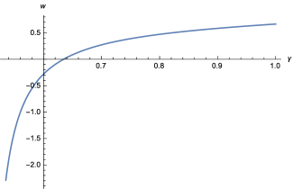
We can find a good estimate of the interval yielding a viable EoS at the present time. Assuming which covers more than present observational bounds, we get
| (20) |
where we have used and and we take , see Figure 1.
Actually for a constant , all background quantities are given in parametric form as follows
| (21) | |||||
| (22) |
with
| (23) |
For in the interval (19), the following consistent limits are indeed obtained
| (24) | |||||
| (25) |
Note that integrability of the problem involved is not restricted to the case of a constant . As was shown in [12], the inverse problem of the determination of the scale factor , the relative Hubble function and the corresponding can be solved explicitly for any given behaviour of .
Inside the interval a phantom behaviour is obtained, with for . Hence for quintessence (a minimally coupled scalar field), for which strong and null energy conditions may not be violated, the interval is excluded and the allowed interval for quintessence reduces to
| (26) |
The value corresponds to . As for , phantom behaviour is unavoidable in the future for the interval (26).
For the specific case , we have , however with . Thus, there are no viable non-tracking quintessence models for which is exactly constant [13].
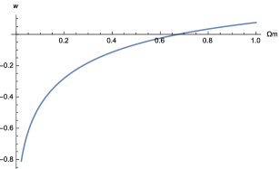
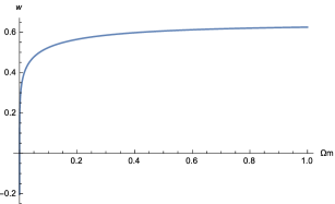
But more interesting cases do exist in the case of tracking DE in the past when . Indeed the roots of the equation determine the cases when DE has a zero pressure deep inside the matter dominated stage so that it is tracking at this stage. This can occur for if . In particular we have the solutions (see Figures 2)
| (27) | |||||
| (28) | |||||
| (29) |
However, while only the upper case (27) is consistent with the strong observational constraints requiring [14], such universes would nevertheless lead to a phantom behaviour in the future, so that quintessence still cannot play the role of DE in (27). This is avoided for (28)-(29), so these solutions are in principle allowed for quintessence. Interestingly, for (28) DE tends to a cosmological constant behaviour in the future, but this model is not viable because would be too small at the matter dominated stage. As increases, this problem becomes sharper. As a corollary, universes with a constant driven by dust and quintessence are mathematically possible but excluded by observations.
Finally, the only way that both and are constant at all times is that be always constant as well. This can only be achieved with which obviously cannot describe our universe dynamics at all times. These universes correspond to the roots of , their expansion is that of Einstein-de Sitter universes. Note that these solutions are unstable, the slightest deviation of , keeping constant, will lead to a varying . To summarize, a constant growth index during the entire evolution of our universe is ruled out for constant and for quintessence.
4 Solving for the evolution of inside GR
While we are mainly interested in a constant and generically cannot be strictly constant forever, it is interesting that many models actually produce a quasi-constant until today. We now turn to the evolution of for some of these models inside GR. Let us consider first the equation governing its dynamics. The simplest way is to write it using the variable . Then we obtain
| (30) |
where we have set
| (31) |
The entire possible evolution of the universe lies in the interval .
Let us start with models having a constant . In this case a constant is obtained numerically in the past starting actually from some low redshifts on. Hence in the past we are in the regime where is constant and we can use (18) in order to relate the initial value with the constant factor . We obtain straightforwardly
| (32) |
Hence the natural thing to do from a mathematical point of view is to solve the exact equation (30) with the initial condition taken at (the asymptotic past). The solution shows a limited departure from around the present-day value . The Taylor expansion around up to second order is given by
| (33) | |||||
The above expression is remarkably accurate. Actually its accuracy is below the percent level already at first order for the present value . This means that we happen to live at the epoch where starts to deviate from a constant behaviour. In order to use the quantity to constrain cosmological models, it will be more convenient to use the redshift , or some other variable closely related to it, instead of . We will return to this point later. Before doing that we will find the value of in the asymptotic future (). This is a mathematically interesting issue. Solving equation (30) in the regime , namely
| (34) |
the following leading order solution is obtained in the future
| (35) |
where is some constant. Hence, tends to the constant value
| (36) |
which corresponds to the particular constant solution of the inhomegeneous equation (34). Obviously, for a non constant with , we simply substitute in (36).
When this value is substituted in (16), corresponding to a constant is recovered. Hence for a given value , the same asymptotic value is obtained in the future whether we assume to be constant or not, viz.
| (37) |
where the left hand side corresponds to a constant and a varying while the right hand side corresponds to the opposite case.
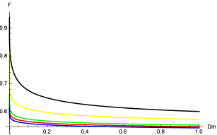
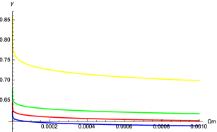
The slope however diverges with
| (38) |
This behaviour is illustrated in Figures 3. The derivative with respect to diverges also. Note that (38) implies that for , as it was emphasized at the end of Section 2 for the quantity to remain finite.
The same procedure can be applied to the asymptotic past . We write (30) in this limit and the solution is then
| (39) |
where is some integration constant. To avoid a singular behaviour, must be set to zero. Here too, corresponds to the particular constant solution of (30) in the limit .
From a practical point of view the use of the redshift rather than is more useful. It is straightforward to rewrite the equation for the evolution of in terms of the variable which yields
| (40) |
Eq.(40) can be solved for models where is known in function of and is dynamical, provided its dynamics in terms of is known as well. Actually, if is known, then the background evolution, and hence , is completely specified.
Let us start with a constant . We can follow the same procedure as before, taking the initial condition (32). Of primary interest for the confrontation with observations is the evolution of around the present time, i.e. around . Written in terms of this expansion becomes
| (41) |
with
| (42) |
The present-day value must be found numerically using Eq.(40). Like for the expansion (33), (41) has an accuracy below the percent level already at first order up to . We stress that is a known function of the underlying parameters and , not an additional free parameter, and in particular that it depends also on .
The useful expansion is really in terms of the variable . The advantages of this variable is well-known in the cosmographic approach, and this variable is actually used for the definition of the (CPL) parametrization [15]
| (43) |
Next step is to consider dynamical dark energy models. Eq.(40) is readily applied to any parametrized model . The motivation here is to use a parametrised expression for the underlying equation of state , and then to use the accurate result (41) instead of looking for some parametrized form for .
It is straightforward to find the first two terms of the expansion (41) for the CPL model. The value has to be found numerically and will depend on both parameters. We can use the same procedure as for a constant EoS in order to find the initial value because in the past tends to a constant value so that we get now
| (44) |
The quantities and depend on both parameters and . In contrast, the coefficient is again given by (42) and does not depend explicitly on (). Indeed the coefficient does not appear explicitly at first order of the expansion (41) for the parametrization (43). The expression (41) here too is very accurate already at first order up to . For example, for and , we obtain numerically . If we use the expansion (41) with (42), one obtains with obtained numerically. One should compare these numbers to the value and we note that is already very close to this value. A variation of the EoS will hardly be observable for a modest change in .
5 A constant growth index beyond GR
As modified gravity DE models are known to allow for an effective DE component of the phantom type [11, 16], they cannot be ruled out for the same reason as quintessence. One could expect that these models offer better prospects to accommodate a constant , possibly with a constant or with tracking DE and we turn now our attention to these questions.
For constant and our starting point is
| (45) |
We see that is again given by (16) with in the interval (17). Looking at the asymptotic past, we obtain
| (46) |
where we have defined
| (47) |
Clearly to avoid that diverges. We have therefore . The condition together with (17) yields
| (48) |
with . For , we have for . As expected, the allowed interval (19) is re-obtained for and for (48) shrinks to zero when . Hence the interval (17) is not necessarily reduced by constraints from the past universe. Further is no longer of the phantom type if , which is possible for .
5.1 A constant
We derive now the condition for to be constant. It is easy to see that this is achieved provided the following equality hold
| (49) |
which constrains the evolution of as follows
| (50) |
As a result of (50) we have for and again when . A powerful constraint on is implied by (50), viz.
| (51) |
In the DE domination it is clear that (50) would be strongly violated for and this violation will be even stronger for . According to Eq.(50), would eventually vanish in a DE dominated universe. We recover in particular the result that a constant growth index is not possible inside GR for a constant equation of state . Interestingly, a value would also increase the r.h.s. of (50) at the present epoch, but cannot have this value during the entire evolution of the universe.
We can also use (50) in a different perspective: knowing that is constant, is it possible to have a constant ? We see from (50) that this is possible for and . So a constant is compatible with a constant inside GR deep in the matter era with and the corresponding is found from eq.(18). It is interesting to relate this result to CDM. On very low redshifts, , we obtain to high accuracy [7] with depending on . While in the DE dominated stage, CDM would violate (50) (with ), on larger redshifts tends to the slightly lower asymptotic value which is essentially reached for confirming our results.
It is also interesting to consider a situation where is constant (but ) on a restricted part of the expansion only which we take around the present time. Then during that stage, the relation (50) taken at the present time is generalized to
| (52) |
where we have defined . Eq.(50) taken today is recovered for . Then again (52) would be generically strongly violated if a constant is kept around the present time. This is particularly interesting for all modified gravity DE models which are known to produce at the present epoch. For example, for , , and , we obtain , still significantly less than one. This is to be compared with for .
We want to comment finally on a possible scale dependence of the growth index. In many modified gravity DE models [16] the appearance of a fifth force, and its effective screening on small scales where this fifth force should not be felt, implies generically a scale dependence of and therefore of the perturbation growth on large cosmic scales. In that case we can still use (45), however for each scale separately and the growth index , though constant in time, will differ for different scales. All the results derived above hold for each scale separately.
Let us now apply our results to some concrete models outside GR. We choose one model, a model based on scalar-tensor gravity where the growth of perturbations deep inside the Hubble radius is scale-independent and another family of models, DE models, where the growth is scale-dependent, too.
a) We consider first the scalar-tensor (ST) DE model considered in [11] with Lagrangian
| (53) |
with a version of this model which is essentially massless on cosmic scales 111One should not confuse with the function introduced in Eq. (13), nor with the growth function introduced in Eq. (4).. In this unscreened version of the model, the quantity affecting the perturbations growth through (8) corresponds also to the gravitational coupling between two test masses in a laboratory experiment and it is given by the expression . Hence its value today is equal to the Newton constant , and we have today . By having today a very large Brans-Dicke parameter , these models obey laboratory and Solar system constraints [17] with . For , Eq.(50) is grossly violated today, so this model cannot accommodate a constant growth index with a constant .
b) An interesting generalization can be given for some modified gravity models like f(R) DE models (see e.g. the review [18]). These models comply with laboratory and Solar system constraints due to screening of the fifth force for scales that are larger than some critical scale . This scale is the Compton length of the scalaron – a scalar degree of freedom, or particle in quantum language, appearing in gravity – which depends on the Ricci scalar and finally on the matter density 222This behaviour is well known in plasma physics (plasmon) and in elementary particle physics, still in cosmology the special term ”chameleon” is often introduced.. Then the growth of matter density perturbations obeys Eq. (8), with being both time and scale dependent. Due to this screening mechanism, reduces to in high curvature regions. Let us see explicitly how this works for viable DE models suggested in the literature. We then have [19, 20]:
| (54) |
In viable models of present DE, all relevant cosmic scales satisfy at the matter era with to high accuracy. In this way the standard growth of perturbations is regained. At low redshifts however, as the critical length increases significantly with the decrease of matter density and the Ricci scalar , for cosmic scales smaller than we will have and matter perturbations on these scales will experience a modified (boosted) growth. As [21, 22] (otherwise a weak curvature singularity appears in solutions), the factor in front of the brackets in (54) increases as the universe expands and it becomes larger than one. So we have for these models for any scale at any time. The quantity becomes as large as in the present era on scales where the growth of matter perturbations is boosted, so that (50) gets strongly violated. Actually, for any modified gravity model with and for in the DE domination, (50) or (52) is strongly violated at the present time. It is interesting in this respect that generalized Proca DE models were recently suggested for which seems possible [23].
5.2 Tracking dark energy in the matter era
While modified gravity DE models with cannot accommodate a constant , let us consider if they allow DE to scale like dust-like matter deep in the matter era with . From (45), the following equation should be satisfied
| (55) |
Equation (55) has solutions only for . It is seen that in this case is no longer constrained to be equal to one. If we take any realistic , but close to , and , a can be found which solves (55)
| (56) |
It is also seen from (56) that is not unique but depends on the model parameters and . In case is scale dependent, (56) should be considered for each scale separately.
We will show now how this can be realized using ST gravity. As was shown in [17], one can construct a so-called asymptotically safe version for which tends in the past to a constant value . So we have in the asymptotic past
| (57) |
the model tends to GR in the past however with the gravitational constant (57) different from its present-day value which is used in the definition of the relative densities . Matter perturbations on scales deep enough inside the Hubble radius in the past obey eq.(8) with a constant given by (57). In this scenario one has deep in the matter era
| (58) |
We get from the modified Friedmann equations
| (59) |
where . Note that Big-Bang nucleosynthesis bound constraints to be close to and we take . So we have in particular
| (60) |
So we see that a constant (56) can be found which is a solution of Eq.(55). Hence on those scales for which matter perturbations satisfy the modified growth of perturbations with constant given by (57), a constant is compatible with DE behaving like dust while .
Interestingly, a second family of tracking solutions are allowed in this model. Indeed, if we take (but again not too much larger), so that now and , (55) will have solutions corresponding to this case too leading to new tracking solutions.
6 Conclusion
In this work we have studied the conditions under which the growth index of scalar (density) perturbations in the non-relativistic matter component in the Universe (cold dark matter and baryons) can be constant in the presence of DE not interacting directly with matter 333For complementary approaches to the growth index and its use, see e.g. [24].. We emphasize that we mean by that the condition for to be strictly constant during the entire evolution of the Universe after the end of the radiation dominated stage. We have also investigated the possibility for DE models to accommodate for both a constant and a constant DE equation of state . It appears that if DE is described by quintessence (a scalar field minimally coupled to gravity) in the GR framework, this behaviour of is excluded either because it would require transition to phantom behaviour of DE at some finite moment of time (which is not possible for quintessence), or, in the case of early (tracking) DE at the matter dominated stage, because the relative matter density appears to be too small. Thus, it seems to be nothing more deep in being exactly constant, and its quasi-constant behaviour in the standard CDM and the simplest quintessence models of DE is simply a consequence of a narrow allowed interval for its variation, Eq. (26), even with adding the case Eq. (27) for early DE. We have found that this is also ruled out in many modified gravity models. We have shown it explicitly for massless scalar-tensor DE models and for the DE models suggested in the literature. In all these models, the condition (50) would be strongly violated at the DE domination, and even stronger on cosmic scales where the growth of matter perturbations is boosted. Assuming around the present time only would still lead to a strong violation of (50) today. It is interesting that in DE models beyond GR allowing , like generalized Proca models, violation of (50) today could be milder. Of course, around the present time is possible in these models if is substantially non constant. We believe that the results obtained here, which relate the behaviour of with the effective gravitational coupling, shed a new light on earlier findings for models [8, 9] where the growth index showed substantial variation already on very low with . This is interesting in particular as a nonstandard behaviour of the growth index could be one of the smoking guns of DE models beyond GR.
Acknowledgments
A.A.S. was partially supported by the grant RFBR 14-02-00894 and by the Scientific Program P-7 of the Presidium of the Russian Academy of Sciences. D.P. acknowledges useful discussions with Stefan Auclair.
References
- [1] V. Sahni and A. A. Starobinsky, Int. J. Mod. Phys. D 9, 373 (2000); P. J. E. Peebles and B. Ratra, Rev. Mod. Phys. 75, 559 (2003); E. J. Copeland, M. Sami and S. Tsujikawa, Int. J. Mod. Phys. D 15, 1753 (2006); V. Sahni and A. A. Starobinsky, Int. J. Mod. Phys. 15, 2105 (2006); M. Li, X.-D. Li, S. Wang and Y. Wang, Commun. Theor. Phys. 56, 525 (2011).
- [2] D. H. Weinberg, M. J. Mortonson, D. J. Eisenstein, C. Hirata, A. G. Riess and E. Rozo, Phys. Rept. 530, 87 (2013); L. Amendola et al., Living Rev. Rel. 16, 6 (2013); P. Bull et al., Phys. Dark Univ. 12, 56 (2016).
- [3] V. Sahni, A. Shafieloo and A. A. Starobinsky, Astrophys. J. 793, L40 (2014).
- [4] P. J. E. Peebles, Astrophys. J. 284, 439 (1984).
- [5] O. Lahav, P. B. Lilje, J. R. Primack and M. J. Rees, MNRAS 251, 128 (1991).
- [6] E. V. Linder and R. N. Cahn, Astropart. Phys. 28 481 (2007).
- [7] D. Polarski and R. Gannouji, Phys. Lett. B 660, 439 (2008).
- [8] R. Gannouji, B. Moraes and D. Polarski, JCAP 0902, 034 (2009).
- [9] H. Motohashi, A. A. Starobinsky and J. Yokoyama, Progr. Theor. Phys. 123, 887 (2010).
- [10] L. Wang and P. J. Steinhardt, Astrophys. J. 508, 483 (1998).
- [11] B. Boisseau, G. Esposito-Farèse, D. Polarski and A. A. Starobinsky, Phys. Rev. Lett. 85, 2236 (2000).
- [12] A. A. Starobinsky, JETP Lett. 68, 757 (1998) [arXiv:astro-ph/9810431].
- [13] A. A. Starobinsky, invited talks at the conferences Cosmology Workshop Montpellier11 (Montpellier, 03.11.2011) and HEA-2011 (Moscow, 14.12.2011), unpublished.
- [14] P. A R. Ade et al., Astron. Astroph. 594, A13 (2016).
- [15] M. Chevallier and D. Polarski, Int. J. Mod. Phys. D10, 213 (2001); E. V. Linder, Phys. Rev. Lett. 90, 091301 (2003).
- [16] T. Clifton, P. G. Ferreira, A. Padilla and C. Skordis, Phys. Rept. 513, 1 (2012); A. Joyce, B. Jain, J. Khoury and M. Trodden, Phys. Rept. 568, 1 (2015).
- [17] R. Gannouji, D. Polarski, A. Ranquet and A. A. Starobinsky, JCAP 0609, 016 (2006).
- [18] A. De Felice and S. Tsujikawa, Living Rev. Rel. 13, 3 (2010).
- [19] P. Zhang, Phys. Rev. D 73, 123504 (2006).
- [20] S. Tsujikawa, Phys. Rev. D 76, 023514 (2007).
- [21] A. A. Starobinsky, JETP Lett.86, 157 (2007).
- [22] S. A. Appleby, R. A. Battye and A. A. Starobinsky, JCAP 1006, 005 (2010).
- [23] A. De Felice, L. Heisenberg, R. Kase, S. Mukohyama, S. Tsujikawa and Y. Zhang, Phys. Rev. D 94, 044024 (2016).
-
[24]
M. Malekjani, S. Basilakos, Z. Davari, A. Mehrabi, M. Rezaei,
Mon. Not. Roy. Astron. Soc. 464, 1192 (2017);
Alberto Bailoni, Alessio Spurio Mancini, Luca Amendola, arXiv:1608.00458;
Xiao-Wei Duan, Min Zhou, Tong-Jie Zhang, arXiv:1605.03947;
B. Wang, E. Abdalla, F. Atrio-Barandela, D. Pavon, Rept. Prog. Phys. 79, no.9, 096901 (2016);
N. Nazari-Pooya, M. Malekjani, F. Pace, D. Mohammad-Zadeh Jassur, Mon. Not. Roy. Astron. Soc. 458, no.4, 3795 (2016);
S. Basilakos, J. Solà, Phys. Rev. D92, no.12, 123501 (2015);
I. de Martino, M. De Laurentis, S. Capozziello, Universe 1, no.2, 123 (2015);
J. N. Dossett, M. Ishak, D. Parkinson, T. Davis, Phys.Rev. D92, no.2, 023003 (2015);
A. B. Mantz et al., Mon. Not. Roy. Astron. Soc. 446, 2205 (2015);
S. Nesseris, S. Basilakos, E.N. Saridakis, L. Perivolaropoulos, Phys. Rev. D88 103010 (2013);
K. Bamba, Antonio Lopez-Revelles, R. Myrzakulov, S.D. Odintsov, L. Sebastiani, Class. Quant. Grav. 30 015008 (2013);
A. Bueno belloso, J. Garcia-Bellido, D. Sapone, JCAP 1110, 010 (2011);
R. Bean, M Tangmatitham, Phys. Rev. D81, 083534 (2010);
Puxun Wu, Hong Wei Yu, Xiangyun Fu, JCAP 0906, 019 (2009);
Seokcheon Lee, Kin-Wang Ng, Phys. Lett. B688, 1 (2010);
Yungui Gong, Phys.Rev. D78, 123010 (2008);
V. Acquaviva, A. Hajian, D. N. Spergel, S. Das, Phys. Rev. D78 043514 (2008);
Hao Wei, Phys. Lett. B664 1 (2008);
S. Nesseris, L. Perivolaropoulos, Phys. Rev. D77, 023504 (2008).