Formation of the helium EUV resonance lines

Abstract

Context. While classical models successfully reproduce intensities of many transition region lines, they predict helium EUV line intensities roughly an order of magnitude lower than the observed value.

Aims. To determine the relevant formation mechanism(s) of the helium EUV resonance lines, capable of explaining the high intensities under quiet sun conditions.

Methods. We synthesise and study the emergent spectra from a 3D radiation-magnetohydrodynamics simulation model. The effects of coronal illumination and non-equilibrium ionisation of hydrogen and helium are included self-consistently in the numerical simulation.

Results. Radiative transfer calculations result in helium EUV line intensities that are an order of magnitude larger than the intensities calculated under the classical assumptions. The enhanced intensity of He I $\lambda 584$ is primarily caused by He II recombination cascades. The enhanced intensity of He II $\lambda 304$ and He II $\lambda 256$ is caused primarily by non-equilibrium helium ionisation.

Conclusions. The analysis shows that the long standing problem of the high helium EUV line intensities disappears when taking into account optically thick radiative transfer and non-equilibrium ionisation effects.

1 Introduction

The formation mechanism of the He i and He ii EUV resonance lines is a topic that has been discussed for many decades. Some of the first calibrated spectral observations of the EUV helium lines, and the EUV wavelength range in general, became available in the sixties around the time when the Orbiting Solar Observatory series of satellites were launched. While models were capable of explaining the intensities of many transition region lines, they did not explain the helium intensities that were observed. In particular, Jordan (1975) found that the observed intensity of these lines were an order of magnitude larger than derived values based on emission measure models. Values in similar ranges have been confirmed also by more recent studies (MacPherson & Jordan, 1999; Pietarila & Judge, 2004; Giunta et al., 2015) using classical modelling similar to that of Jordan (1975). Pinning down the relevant formation mechanism(s) of the helium lines is important because it will help guide interpretations of observations.

A possible intensity enhancement mechanism was suggested already by Jordan (1975). The collisional excitation rate of the helium resonance lines are highly sensitive to temperature. She therefore proposed that if cold ions in some way got mixed with hot electrons, more photons would be produced. One possible physical mechanism that would create such a mix is particle diffusion. This was added by Fontenla et al. (1990, 1991, 1993) in a semi-empirical 1D model, and gave enough intensity in the hydrogen Lyman-$\alpha$ without the need to for the temperature plateau at 20 kK present in the Vernazza et al. (1981) models. Another mechanism is the so called velocity redistribution (VR) (Jordan, 1980) which was also investigated by Andretta et al. (2000) who invented the term VR, Smith & Jordan (2002), and Pietarila & Judge (2004). The driver of the latter mechanism is turbulent fluid motions that transport cold atoms into hotter regions. While both the particle diffusion and the VR mechanisms do enhance the helium EUV line intensities, they affect only the photon production due to collisional excitation.

Another suggested mechanism is the photoionisation-recombination (PR) mechanism (Zirin, 1975, 1996). In short; half of the EUV photons emitted in transition region and coronal lines will be lost into space and the other half will constitute a coronal illumination of the chromosphere and be absorbed in the continua of either helium or hydrogen. The resulting photoionised helium atoms will recombine and de-excite through a cascade event, and ultimately emit a helium resonance photon. In such a scenario more EUV photons emitted from the corona would increase the number of helium resonance line photons produced. Andretta & Jones (1997) investigated this idea and found that incident radiation from the corona could enhance the line intensity of He i $\lambda$584 in very quiet regions, but had a marginal effect on more active regions. Later he also found that the PR mechanism can not be the primary formation mechanism of He ii $\lambda$304 in quiet regions (Andretta et al., 2003). The subordinate helium lines, however, have been shown to be sensitive to coronal illumination (Wahlstrom & Carlsson, 1994; Avrett et al., 1994; Andretta & Jones, 1997; Mauas et al., 2005; Centeno et al., 2008; Leenaarts et al., 2016).

In this paper we study the formation of the helium EUV resonance lines by exploiting state-of-the-art 3D numerical models and 3D non-LTE radiative transfer including the effects of non-equilibrium ionisation. The paper is laid out as follows: in Sec. 2 we describe our method of computing the line intensities, in Sec. 3–4 we describe our model atom and model atmosphere, in Sec. 5 we follow a classical approach and assess the helium line enhancement calculated from our model, in Sec. 6 we describe how the helium resonance lines are formed in the model, and in Sec. 7 we discuss our results. Finally, in Sec. 8 we summarise and draw conclusions.

2 Method

We compare and investigate line intensities from the solar atmosphere at disc centre ($\mu=1$). The line intensity, $I$, is given by the frequency integral over the specific intensity emerging from the atmosphere, $I_{\nu}(\mu)$,

$$I=\int_{D}I_{\nu}(\mu=1)\,\mathrm{d}\nu,$$ (1)

where $\nu$ is frequency and $D$ denotes the frequency domain relevant for the line under consideration. $I_{\nu}(\mu)$ is the solution of the equation of radiative transfer

$$\frac{\mathrm{d}I_{\nu}}{\mathrm{d}s}=\eta_{\nu}-I_{\nu}\chi_{\nu},$$ (2)

where $s$ is the distance along a ray, $\eta_{\nu}$ and $\chi_{\nu}$ are the frequency dependent emissivity and opacity, respectively. In Sec. 2.1 and 2.2 we describe how we solve Eq. 2.

2.1 Non-equilibrium radiative transfer with Multi3d

We use Multi3d (Leenaarts & Carlsson, 2009) to solve the equation of radiative transfer coupled to a particle conservation equation and a set of equilibrium rate equations. The transfer equation is solved using an extremum-preserving third order Hermite interpolation scheme (e.g. Ibgui et al., 2013). The code solves the rate equations using the formulation of Rybicki & Hummer (1991, 1992)

Given a model atom with $N$ atomic states constituting $M$ ion stages and a set of transitions, the statistical equilibrium rate equations take the form

$$\sum_{j=1,j\neq i}^{N}n_{j}P_{ji}-n_{i}\sum_{j=1,j\neq i}^{N}P_{ij}=0,$$ (3)

where $P_{ij}$ is the rate coefficient giving the probability per unit time of a transition from the $i$-th to the $j$-th state. In principle it is possible to express $N$ equilibrium rate equations, but they constitute a linearly dependent set of equations which is why we replace one of them by the particle conservation equation,

$$\sum_{i=1}^{N}n_{i}=n,$$ (4)

where $n$ is proportional to the mass density by an abundance dependent factor. We refer to the intensity calculated with this setup, solving the radiative transfer equation (Eq. 2) together with $N-1$ rate equations (Eq. 3) and one particle conservation equation (Eq. 4), as the non-LTE solution (NLTE).

We know that non-equilibrium effects on the helium lines are lost in the NLTE solution (Golding et al., 2014). In that paper we also showed that the processes that affect the ionisation state of helium are slow compared to the processes that populate the excited states. We can therefore approximate non-equilibrium effects by constraining the radiative transfer solution by non-equilibrium ion fractions (for an analysis of the time-dependent rate equations in evolving plasmas see Judge, 2005). We do this by solving the equilibrium rate equations (Eq. 3) for the $N-M$ excited states of the atom. The $M$ ion fraction equations replace the ground state rate equations. Let $f_{j}$ denote the fraction of atoms in the $j$-th ion stage. The ion fraction equations then take the form

$$\sum_{i=1}^{N}n_{i}d_{ji}=f_{j}n$$ (5)

where $d_{ij}=1$ if $i$ is a state in the $j$-th ion stage and $d_{ij}=0$ if $i$ is not a state in the $j$-th ion stage. We modify Multi3d so that it solves this alternative set of equations when ion fractions are given as input. We refer to the solution of this set of equations as the non-equilibrium non-LTE solution (NE-NLTE).

2.1.1 Test of the non-equilibrium non-LTE radiative transfer

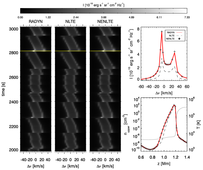
Figure 1: Emergent He I $\lambda 584$ line profiles from the Radyn simulation compared to the NLTE and NE-NLTE radiative transfer solutions from Multi (three left panels). The top right panel shows the line profile in the three approaches for the snapshot indicated by the yellow lines. The bottom right panel shows the number density of the upper level of the transition in the three approaches. The grey line shows the temperature with scale to the right.

We now check whether the method described in Sec. 2.1 for computing the NE-NLTE solution matches the emergent intensity of a dynamic solar atmosphere model. Such a test can only be carried out in a 1D geometry because it is not possible with contemporary computer resources to construct a dynamic 3D model with a self-consistent time dependent non-LTE description of the radiative transfer.

The dynamic solar atmosphere model is computed with the radiation-hydrodynamics code Radyn (Carlsson & Stein, 1992, 1995, 1997, 2002). Radyn solves the conservation equations of mass, momentum, charge, and energy, as well as the radiative transfer equation (Eq. 2) and a set of non-equilibrium rate equations for the atomic number densitites.

$$\frac{\mathrm{d}n_{i}}{\mathrm{d}t}+\nabla\cdot(\mathbf{v}n_{i})=\sum_{j=1,j\neq i}^{N}n_{j}P_{ji}-n_{i}\sum_{j=1,j\neq i}^{N}P_{ij},$$ (6)

where $\mathbf{v}$ is the bulk velocity.

We use the NE-run from Golding et al. (2014) as a reference model. Each snapshot of the reference model describes the state of the atmosphere at a given time. For each snapshot we write input files for the 1D radiative transfer code Multi (Carlsson, 1986) and compute the NLTE solution. The modifications made to Multi3d are made also in Multi. Non-equilibrium ion fractions, $f_{j}$, are available from the reference Radyn model. We use these as input together with the Multi input files and for each snapshot compute the NE-NLTE solution with the modified version of Multi.

In Fig. 1 we compare the time dependent emergent intensity of the He I $\lambda 584$ resonance line with the results from the NLTE and NE-NLTE solutions. The sawtooth pattern due to shocks is evident in all three intensities. The NE-NLTE solution reproduces the intensity brightenings occurring at the onset of some of shocks. This is a non-equilibrium effect and it is not recovered in the NLTE solution. The He II $\lambda 304$ line has brightenings as well (shown in Figure 8 of Golding et al. (2014)), and also these are reproduced in the NE-NLTE solution and lost in the NLTE solution (not shown here).

From this we conclude that the NE-NLTE method implemented in Multi3d will produce relevant non-equilibrium effects on the helium spectrum, given the appropriate non-equilibrium ionisation state as input.

2.2 Optically thin line formation

Assuming optically thin conditions we neglect the last term of Eq. 2. In this case the line intensity becomes a simple line-of-sight integral along the ray $S$,

$$I_{\mathrm{th}}=\int_{S}\eta\ \mathrm{d}s,$$ (7)

where $\eta$ is the frequency-integrated line emissivity given by $\eta=\int_{D}\eta_{\nu}\ d\nu$. The frequency integrated emissivity can be expressed as

$$\eta=A_{ul}\left(\frac{h\nu_{0}}{4\pi}\right)\left(\frac{n_{u}}{n_{\mathrm{ion}}}\right)\left(\frac{n_{\mathrm{ion}}}{n_{\mathrm{el}}}\right)\left(\frac{n_{\mathrm{el}}}{n_{\mathrm{H}}}\right)n_{\mathrm{H}},$$ (8)

where $A_{ul}$ is the Einstein coefficient for spontaneous radiative de-excitation, $h$ is Planck’s constant, $\nu_{0}$ is the frequency of the line, $n_{u}$ is the number density of atoms in the upper level of the line, $n_{\mathrm{ion}}$ is the number density of atoms in the ion stage, $n_{\mathrm{el}}$ is the number density of atoms of the element, and $n_{\mathrm{H}}$ is the number density of hydrogen atoms. This expression is general; $n_{u}$ is dependent on the intensity, as well as $n_{\mathrm{e}}$ and $T$. However, under optically thin conditions $n_{u}$ looses its dependency on the intensity. If we in addition assume that

• the processes that are affecting $n_{\mathrm{ion}}$ are independent of the processes affecting the number densities of the excited states within an ion stage,

• the system is in a steady state condition,

then the evaluation of Eq. 8 becomes simple. We will refer to these three assumptions collectively as the optically thin equilibrium approximation. The fraction $(n_{u}/n_{\mathrm{ion}})$ is then found by solving a set of equilibrium rate equations (Eq. 3) and a normalised particle conservation equation (Eq. 5 divided by $n_{\mathrm{ion}}$). The transition rate coefficients are only made up of terms involving collisional excitation, collisional de-excitation and spontaneous radiative de-excitation. The collisional terms are expressed by $n_{\mathrm{e}}q(T)$, where $q(T)$ is dependent on the specific transition. The radiative spontaneous de-excitation rate is given by the Einstein $A_{ul}$ coefficient. The ionisation equilibrium fraction, $(n_{\mathrm{ion}}/n_{\mathrm{el}})$, is found in a similar way. The transition rate coefficients are in this case made up of terms made up of collisional ionisation, di-electronic recombination and spontaneous radiative recombination. All of these terms are linear in $n_{\mathrm{e}}$, and this makes $(n_{\mathrm{ion}}/n_{\mathrm{el}})$ dependent on temperature only. Under the optically thin equilibrium approximation we denote these two fraction as $(n_{\mathrm{u}}/n_{\mathrm{ion}})_{\mathrm{eq}}$ and $(n_{\mathrm{ion}}/n_{\mathrm{el}})_{\mathrm{eq}}$. The optically thin equilibrium emissivity, $\eta_{\mathrm{eq}}$, is then expressed as

$$\eta_{\mathrm{eq}}=G(T,n_{\mathrm{e}})\,n_{\mathrm{e}}n_{\mathrm{H}},$$ (9)

where $G(T,n_{\mathrm{e}})$ is defined as

$$G(T,n_{\mathrm{e}})=\left(\frac{A_{ul}}{n_{\mathrm{e}}}\right)\left(\frac{h\nu_{0}}{4\pi}\right)\left(\frac{n_{u}}{n_{\mathrm{ion}}}\right)_{\mathrm{eq}}\left(\frac{n_{\mathrm{ion}}}{n_{\mathrm{el}}}\right)_{\mathrm{eq}}\left(\frac{n_{\mathrm{el}}}{n_{\mathrm{H}}}\right).$$ (10)

This function will typically have only a weak dependence on $n_{\mathrm{e}}$ and be sharply peaked in temperature. We will refer to the temperature where $G$ peaks as the formation temperature of the line.

2.2.1 Differential emission measure modelling

A differential emission measure distribution (DEM), $\Phi(T)$, gives an indication of how much radiating material is present at different temperatures of a solar region or feature. It is defined as,

$$\Phi(T)=n_{\mathrm{H}}n_{\mathrm{e}}\frac{\mathrm{d}z}{\mathrm{d}T}.$$ (11)

It can be used to compute the thin line intensities under equilibrium conditions,

$$I_{\mathrm{DEM}}=\int_{T}G(T,n_{\mathrm{e}})\Phi(T)\ \mathrm{d}T$$ (12)

When a set of line intensities are known, it is possible to invert this equation and obtain an estimate of $\Phi(T)$ (see for example Cheung et al., 2015, and references therein). Since $G$ is also a (weak) function of $n_{\mathrm{e}}$ this requires an assumption about the electron density as function of temperature. A common assumption is to use a constant electron pressure, $P_{\mathrm{e}}=k_{\mathrm{B}}n_{\mathrm{e}}T$, where $k_{\mathrm{B}}$ is Boltzmann’s constant.

3 Helium model atom

We use a 13 level helium model atom to perform radiative transfer calculations. It has nine He i states, three He ii states and the fully ionised state He iii. To construct the 13 level model atom we used the 33 level helium model atom from Golding et al. (2014) as a basis. For He i we kept the ground state $n=1$ and six $n=2$ excited states unchanged. All singlet $n=3$ states were merged to one representative state. This was also done for all triplet $n=3$ states. All the He i excited states with $n\geq 4$ were neglected. For He ii we kept the ground state $n=1$ unchanged. All the $n=2$ states were merged to one representative state, and all the $n=3$ states were merged to one representative state. He ii excited states with $n\geq 4$ were neglected. The helium abundance is set to 0.1 helium atoms per hydrogen atom.

4 Model atmosphere

As our model atmosphere we use a snapshot from a 3D radiation-magnetohydrodynamic simulation. The simulation was run with the code Bifrost (Gudiksen et al., 2011) and features non-equilibrium ionisation of hydrogen (Leenaarts et al., 2007) and helium (Golding et al., 2016). The ionisation state of helium is strongly dependent on the radiative losses from the transition region and corona (EUV photons) which leads to photoionisation in the chromosphere. The radiative losses are taken into account in the simulation and they self-consistently give rise to the coronal illumination. Other than the non-equilibrium helium ionisation the simulation has the same setup as the enhanced network simulation described in Carlsson et al. (2016). The spatial domain of the simulation is $24\times 24\times 17$ Mm³, spanning from the convection zone at $z=-2.5$ Mm to the corona at $z=14.5$ Mm. $z=0$ Mm is defined as the average height where the the optical depth at 5000 Å is unity. The simulation has a resolution of $504\times 504\times 496$ grid points. The snapshot we use as the model atmosphere represents the physical state of the atmosphere about 20 minutes after the non-equilibrium ionisation was switched on. This is long enough for potential startup effects to have vanished. According to figures shown in Golding et al. (2016), the ionisation state of helium relaxes to chromospheric conditions on timescales of about 10-15 minutes. The simulation provides all the quantities that we need ($\rho$, $\mathbf{v}$, $T$, $n_{\mathrm{e}}$, $n_{i}$ of hydrogen, and $f_{j}$ of helium) at each grid point of the snapshot.

5 Enhancement factors and the classical approach

Table 1: Helium line enhancement factors from different studies.

Study	He i $\lambda$584	He ii $\lambda$304	He ii $\lambda$256
Jordan (1975)	15	5.5
MacPherson & Jordan (1999)	10-14	13-25
Pietarila & Judge (2004)	2-10	27
Giunta et al. (2015)	0.5-2	13	5
This work	7	10	7

We will follow a similar procedure to that of Giunta et al. (2015). In short, they observed a set of lines with formation temperatures in the range ¹⁰log$(T)=4.3$ to 6.25, including resonance lines of He i and He ii. Line intensities were spatially and temporally averaged. Based on a subset of these line intensities they inverted Eq. 12 to obtain a DEM. Then they used the derived DEM to compute the intensities of all the observed lines, $I_{\mathrm{DEM}}$ (also with Eq. 12). The discrepancy between observed and modelled line intensities was quantified by an enhancement factor defined as the ratio of the observed intensity to the DEM-modelled intensity. For most of the lines the enhancement was around one, except for a few lines including the resonance lines of He ii. Similar studies have have been conducted also by others (Jordan, 1975; MacPherson & Jordan, 1999; Pietarila & Judge, 2004). In Table 1 we sum up their resulting enhancement factors for the helium lines.

The lines observed by Giunta et al. (2015) are listed in their Table 2, 3, and 4. We compute the line intensities for all of the listed lines assuming optically thin equilibrium conditions (defined in Section 2.2). For He I $\lambda 584$, He II $\lambda 304$, and He II $\lambda 256$ we also compute the NE-NLTE thick line intensities.

5.1 Thin calculations

We assume optically thin equilibrium conditions and compute the EUV line intensities with Eq. 7 from all the columns of the model atmosphere. To obtain the equilibrium line emissivities, $\eta_{\mathrm{eq}}$, of the various lines on each point of the model atmosphere we exploit the atomic database and software tools from the Chianti package (Dere et al., 1997; Del Zanna et al., 2015). We use the chianti.ioneq ionisation equilibrium file and coronal abundances from Schmelz et al. (2012). For He I $\lambda 584$, He II $\lambda 304$, and He II $\lambda 256$ we use the helium model atom described in Section 3 to calculate $\eta_{\mathrm{eq}}$. These thin intensities are denoted $I_{\mathrm{th}}$.

5.2 Thick calculations

We run the NE-NLTE mode of Multi3d to compute the non-equilibrium helium line intensities from the model atmosphere. To make the problem computationally tractable we halved the horizontal resolution of the model atmosphere so that it is given on a $252\times 252\times 496$ grid. The line intensities computed are He i $\lambda$584, He ii $\lambda$304, and the He ii $\lambda$256. These line intensities are denoted $I_{\mathrm{RT}}$.

5.3 Verification of the model atmosphere

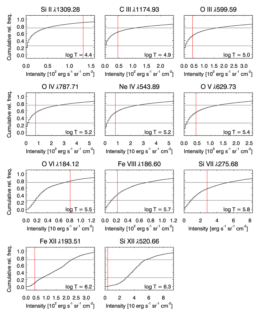
Figure 2: Cumulative distributions of thin line intensities, $I_{\mathrm{th}}$, computed from the model atmosphere. Horizontal lines in each panel indicate the location of the first and third quartile. Red vertical lines indicate the observed values.

To assess how well our model atmosphere represents solar transition region and coronal conditions we compare our intensity, $I_{\mathrm{th}}$, with observed values. The selection of lines and their observed values are listed in Table 7 of Giunta et al. (2015). These are the lines they used to derive their DEM distribution, and they are selected to span a large temperature range. The observed values are of a quiet sun region.

Figure 2 shows the cumulative distribution of $I_{\mathrm{th}}$ for the selected lines. The red vertical line in each panel indicates the observed value, and the horizontal grey lines show the first and third quartile. Our model seem to produce reasonable intensities compared to the observations in most of the lines shown. There are exceptions in the low and high temperature ends. The synthetic intensities of the low temperature Si ii $\lambda$1309 line are likely not very realistic since this line does not form under optical thin conditions (Lanzafame, 1994). The observed intensity of the high-temperature Si xii $\lambda$520 line is far below the interquartile range of the synthetic intensity distribution. However, since the model atmosphere represents an enhanced network region, we expect there to be more hot plasma present than what is the case for quiet sun conditions, and thus higher synthetic intensities of the hot lines.

The model atmosphere produces transition region and coronal line intensities of the same order of magnitude as what is observed in quiet sun regions. We therefore conclude that our model is suitable for a study of the helium EUV resonance lines under quiet sun conditions.

5.4 Deriving the DEM from the model atmosphere

Table 2: Line ratios used to estimate the electron pressure.

Lines	${}^{10}\log{T_{\mathrm{max}}}$	Ratio	$n_{\mathrm{e}}$	$n_{\mathrm{e}}T$
	(K)		(1010 cm-3)	(1015 cm-3K)
O v 762.0 / 629.7	5.4	0.02	1.3	3.12
Si vii 275.3 / 275.7	5.8	5.6	0.3	1.61
Fe xii 193.5 / 186.9	6.2	1.9	0.1	1.67

Figure 3: Differential emission measure derived from the model atmosphere. The DEM is derived from the intensities of the lines shown in Fig. 2

We follow Giunta et al. (2015) and derive a DEM based on a spatial average of our computed line intensities, $\langle I_{\mathrm{th}}\rangle$. We use three density-sensitive line ratios to estimate the electron density at three different temperatures. The density sensitive line ratios and their values are listed in Table 2. These are the same line ratios as the ones used by Giunta et al. (2015). The electron pressure varies less than the electron density over the temperature range. For this reason we use the average electron pressure of $P_{e}/k_{\mathrm{B}}=n_{\mathrm{e}}T=2\times 10^{15}$ cm^-3 K to derive the DEM. The line intensities we use to derive the DEM are the eleven lines shown in Figure 2. To perform the inversion we use the XRT inversion code included in the Chianti package (Dere et al., 1997; Del Zanna et al., 2015). The resulting DEM is shown in Fig. 3.

5.5 Enhancement factors

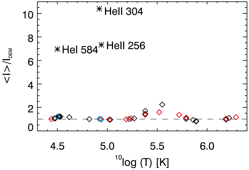
Figure 4: Enhancement factors for all the modelled lines. The lines selected for DEM inversion are indicated by red diamonds. The helium lines are indicated by the black stars. The blue diamonds show the enhancement factors for the helium lines if we use their optically thin equilibrium intensity as the ’observation’. The black diamonds show the enhancement factor for all the other lines included in the study.

We calculate the modelled line intensities, $I_{\mathrm{DEM}}$, with Eq. 12 assuming a constant electron pressure (equal to the pressure used to derive the DEM). Figure 4 shows the synthetic enhancement factor, $\langle I_{\mathrm{th}}\rangle/I_{\mathrm{DEM}}$, for all our included lines, except the helium lines where the enhancement factor is computed by $\langle I_{\mathrm{RT}}\rangle/I_{\mathrm{DEM}}$. They are given as a function of formation temperature. Our DEM distribution successfully reproduces the observed intensities for most of the lines, also those not included for the DEM inversion (indicated by the black diamonds). The helium lines stand out with enhancement factors of about 7 for He i $\lambda$584 and He ii $\lambda$256, and 10 for He ii $\lambda$304. These values are comparable to values reported in earlier studies (see Table 1). We therefore consider the long standing problem of the anomalous helium line intensities in the quiet sun as solved. The helium enhancement factors are caused by optically-thick radiative transfer effects and/or the effects of non-equilibrium ionisation. In the next section we investigate which effects are important for the formation of He I $\lambda 584$, He II $\lambda 256$, and He II $\lambda 304$.

6 Relevant effects for the line intensities

Table 3: Ratios of average line intensities illustrating the effect of thick radiative transfer.

Ratio	He i $\lambda$584	He ii $\lambda$304	He ii $\lambda$256
$R_{\mathrm{DEM}}$	0.14	0.096	0.14
$R_{\mathrm{th}}$	0.18	0.097	0.14
$R_{\mathrm{th,NE}}$	0.097	0.31	0.61

We found in the previous section that the spatially averaged intensity, $\langle I_{\mathrm{RT}}\rangle$, is higher than what we obtain from the DEM distribution. Compared to the simple 1D DEM thin line formation, we are including much more physics in the full NE-NLTE radiative transfer case. Among these ingredients are multidimensional atmospheric structure and a non-equilibrium ionisation state. Ignoring radiative transfer effects, we begin this analysis by testing whether the enhanced intensity can be due to these two ingredients.

First we asses how the 3D atmospheric structure alters the helium line intensity. The intensities computed by line-of-sight integration (Eq. 7) assuming optically thin equilibrium conditions include possible effects of such structure since the emissivity is calculated for each grid point in the model atmosphere based on the local values of temperature and electron density. To quantify the effect we define the line intensity ratios,

$$R_{\mathrm{DEM}} = \frac{I_{\mathrm{DEM}}}{\langle I_{\mathrm{RT}}\rangle}$$ (13)

$$R_{\mathrm{th}} = \frac{\langle I_{\mathrm{th}}\rangle}{\langle I_{\mathrm{RT}}\rangle}.$$ (14)

The values of the ratios for the helium lines are given in Table 3. $R_{\mathrm{DEM}}$ is the inverse of the enhancement factor, and it has a value lower than 1 for the three helium lines considered. The values of $R_{\mathrm{th}}$ are very similar to the values of $R_{\mathrm{DEM}}$. This means that the helium line intensities derived from the DEM approximately reproduce the spatial average of the helium line intensities under optically thin equilibrium conditions. Or in other words, the multidimensional atmospheric structure does not explain the enhanced intensity.

Next we check the effect of non-equilibrium helium ionisation. To do this we compute the optically thin non-equilibrium intensities, $I_{\mathrm{th,NE}}$. These intensities are calculated using the line-of-sight integration in Eq. 7 of the thin non-equilibrium emissivity, $\eta_{\mathrm{neq}}$, which features the same excitation mechanism as the thin equilibrium emissivity, $(n_{\mathrm{u}}/n_{\mathrm{ion}})_{\mathrm{eq}}$, but we let the ion fraction be given by the non-equilibrium value from the model atmosphere, $(n_{\mathrm{ion}}/n_{\mathrm{el}})_{\mathrm{neq}}$. Then we can express the emissivity,

$$\eta_{\mathrm{neq}}=\frac{(n_{\mathrm{ion}}/n_{\mathrm{el}})_{\mathrm{neq}}}{(n_{\mathrm{ion}}/n_{\mathrm{el}})_{\mathrm{eq}}}\ \eta_{\mathrm{eq}}$$ (15)

We are interested in how the spatial average of the thin non-equilibrium line intensity differs from its equilibrium counterpart. We therefore define the ratio

$$R_{\mathrm{th,NE}}=\frac{\langle I_{\mathrm{th,NE}}\rangle}{\langle I_{\mathrm{RT}}\rangle}.$$ (16)

The values of this ratio are given in Table 3.

Figure 5: Details on the thin line formation of He i $\lambda$584 (left column) and He ii $\lambda$304 (right column). Upper panels: line emissivities (solid, scale to the left) and temperature (dashed, scale to the right). Bottom panels: ion fractions (solid, scale to the left) and temperature (dashed, scale to the right). The black lines show the values corresponding to ionisation equilibrium and the blue lines show the values corresponding to non-equilibrium ionisation.

Compared to $R_{\mathrm{th}}$, $R_{\mathrm{th,NE}}$ is halved for the He I line and increased by a factor of three for the He II lines. In other words, if the lines are only excited by collisions, taking the non-equilibrium ionisation state into account results in fewer He I $\lambda 584$ photons and more He II $\lambda 304$ and He II $\lambda 256$ photons than what is predicted by assuming ionisation equilibrium (as described in Section 2.2). Figure 5 shows the ion fractions and corresponding emissivities for the He I $\lambda 584$ and He II $\lambda 304$ lines in a network region column. We choose a network region column because the network regions feature the strongest emission and contribute the most to the averages that goes into $R_{\mathrm{th}}$, and $R_{\mathrm{th,NE}}$. We inspected a representative sample of columns in the snapshot, and they all behave qualitatively the same. The non-equilibrium He I ion fraction is lower than the ionisation equilibrium value, and this makes the non-equilibrium He I $\lambda 584$  emissivity lower. It is opposite for the He II $\lambda 304$ emissivity; the non-equilibrium He ii ion fraction has a tail that reaches into the high temperature transition region (at roughly $z=2.68$ Mm) which results in a non-equilibrium emissivity higher than the corresponding equilibrium value.

$I_{\mathrm{RT}}$ and $I_{\mathrm{th,NE}}$ are computed from an identical atmosphere model and with identical ion fractions. Optically-thick radiative transfer effects therefore remain the only reason why $R_{\mathrm{th,NE}}$ is not equal to one. The ratio is closer to one for the He ii lines than for the He i line. This suggests that the radiative transfer effects are more important for the latter.

6.1 Radiative transfer effects on the He EUV lines

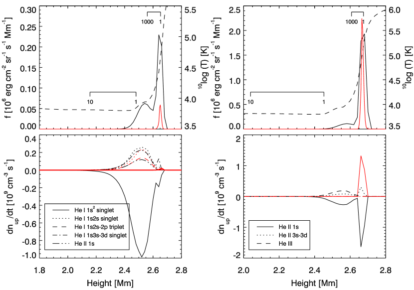
Figure 6: Comparison of the NE-NLTE thick and non-equilibrium thin line formation of He i $\lambda$584 (left column) and He ii $\lambda$304 (right column). Upper panels: contribution functions (scale to the left) for thick formation (solid black) and thin formation (solid red). For context the temperature is also shown (dashed curve, scale to the right). Two additional scales are drawn in each of the two upper panels. The upper scale shows the optical depth at line center. The lower scale shows the optical depth for the continuum. Bottom panels: net rates into the upper level of the transition. Collisional processes are indicated by red lines and radiative transitions are indicated by black lines.

We now turn to the optically thick formation of the helium EUV line intensities. Fig. 6 shows the details for a network column (the same one as in Fig. 5). Here we display a contribution function, $f(z)$. It represents the contribution to the total line intensity as a function of height. We define it by using the formal solution of Eq. 2 (Mihalas, 1978, page 38) to rewrite Eq. 1,

$$I = \int_{D}I_{\nu}\ \mathrm{d}\nu$$ (17)

$$= \int_{D}\int_{\tau_{\nu}}S_{\nu}e^{-\tau_{\nu}}\ \mathrm{d}\tau_{\nu}\ \mathrm{d}\nu$$

$$= \int_{D}\int_{z}\eta_{\nu}e^{-\tau_{\nu}}\ \mathrm{d}z\ \mathrm{d}\nu$$

$$= \int_{z}\int_{D}\eta_{\nu}e^{-\tau_{\nu}}\ \mathrm{d}\nu\ \mathrm{d}z$$

$$= \int_{z}f(z)\ \mathrm{d}z$$

The contribution function is equal to the emissivity (Eq. 8) when the line formation is thin.

First we consider the He I $\lambda 584$ line. The thick contribution function has a larger value than the thin contribution function at all depths where it is significant. It is also more extended in space. The number of photons released in the transition is closely related to the number density of atoms in the excited state (Eq. 8). In the lower panel we therefore show which processes populate the upper level of the transition in the thick calculation. Practically all of the transitions into the upper level are balanced by a radiative de-excitation releasing a He I $\lambda 584$ photon. There is some collisional excitation in the transition region above $z=2.6$ Mm (which causes all of the emission in the thin calculation). The dominant processes in the chromosphere below are radiative transitions from higher energy singlet states and collisional transitions from the triplet states. There is also a significant net radiative rate into the upper state from the lower energy singlet state 1s2s. The singlet state 1s2s is populated mainly by collisions from the triplet states (not shown in figure). In the chromosphere the triplet states are populated mainly by recombinations from He ii 1s (e.g., Andretta & Jones, 1997; Centeno et al., 2008). This means that a significant amount of the He I $\lambda 584$ photons are due to recombination from singly ionised helium followed by a cascade down to the upper level of the line transition, either through the singlet system or the triplet system. Recombination into excited states is not included in thin modelling. A DEM analysis would therefore never account for these photons.

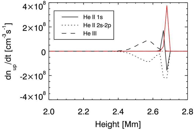
Figure 7: Net rates into upper level of the He ii $\lambda$256 line transition. The red lines indicate collisional transitions. The black lines indicate radiative transitions.

Next we consider the He II $\lambda 304$ line. The thick contribution function is more extended in height than the thin contribution. But both the thin and thick contribution functions peak in the transition region. The thin $f$ has a higher peak than the thick $f$ because it is not depressed by optical depth effects. The dominant process populating the upper level of the transition where the contribution function is significant, is collisional excitation from the He ii ground state. There is a smaller contribution to the total He II $\lambda 304$ line intensity that comes from the chromosphere. Here recombination of He iii dominates in populating the excited state.

For the He II $\lambda 304$ line there are two radiative transfer effects at play: The first one is backscattering of photons. When a collisionnally excited He ii ion de-excites, it releases a photon that travels either up into space or down towards the chromosphere. The line opacity in the chromosphere is high and the photon destruction probability is low. The photon will thus be scattered around. Since the destruction probability is low, a large fraction of the downward-emitted photons will eventually escape upwards into space.

Under idealised conditions, where the photon production happens in a truly thin layer and the destruction probability is zero, all photons eventually escape, and therefore $\langle I_{\mathrm{RT}}\rangle=2\langle I_{\mathrm{th,NE}}\rangle$ and $R_{\mathrm{th,NE}}=0.5$ . Under realistic conditions, the proportionality constant is smaller than two.

The calculated value of $R_{\mathrm{th,NE}}$ is lower than 0.5, or equivalently $\langle I_{\mathrm{RT}}\rangle>2\langle I_{\mathrm{th,NE}}\rangle$, which means that backscattering alone is not sufficient. We explain this by the second effect which is the recombination from He iii. The last step of the recombination cascade produces a He II $\lambda 304$ photon. These photons are primarily created in the optically thick chromosphere. They are released into space after a sequence of scattering steps and add to the thick line intensity.

Turning finally to the He ii $\lambda$256 we have $R_{\mathrm{th,NE}}=0.61$. This line is also optically thick in the chromosphere so we expect that the backscattering effect is important. Since $R_{\mathrm{th,NE}}$ is significantly higher than 0.5, a fraction of the line photons must be destroyed. Figure 7 shows the net rates into to excited state of the line in the same network column as shown in Figure 6. Indeed, He II $\lambda 256$ photons are absorbed and transformed into He ii Balmer-$\alpha$ (and later 304) photons. The dominant processes populating the upper level of the line are otherwise very similar to those populating the excited state of the He II $\lambda 304$ line, with the recombination of He iii in the chromosphere. However, this recombination is the beginning of the downward cascade and the production of a He ii Balmer-$\alpha$ photon and a He II $\lambda 304$ photon.

To sum up we find that the He i $\lambda$584 line is in large part formed by recombination cascades and that the resonance lines of He ii are mostly collisionally excited. We have found this based on radiative transfer modelling where we have taken time dependent ionisation driven by coronal illumination into account. Next we evaluate the effect of how time dependence and coronal illumination affect the intensities of the helium EUV resonance lines.

6.2 Non-equilibrium effects

Table 4: Ratios of average line intensities illustrating the effect of non-equilibrium ionisation.

Ratio	He i $\lambda$584	He ii $\lambda$304	He ii $\lambda$256
$R_{\mathrm{RTE}}$	0.88	0.52	0.57

Figure 8: Details on the He ii $\lambda$304 thick line formation under equilibrium and non-equilibrium conditions. Upper panel: contribution functions (solid lines, scale to the left) and temperature (dashed line, scales to the right). Lower panel: Fraction of He as He ii (solid lines, scale to the left) and temperature (dashed line, scales to the right).

To identify the non-equilibrium effects inherent in $I_{\mathrm{RT}}$ we compute an equilibrium solution $I_{\mathrm{RTE}}$ and compare the two. The equilibrium solution is computed by using equilibrium ion fractions as constraints in the NE-NLTE mode of Multi3d. The equilibrium ion fraction are computed on the basis of the coronal illumination present in the Bifrost simulation. The simulation uses a 3-level helium model atom. To advance the atomic populations, Bifrost computes the radiative and collisional ionisation and recombination transition rate coefficients for every time step. The radiative ionisation coefficient indirectly contains the coronal illumination. We obtain the equilibrium ion fractions by using the radiative and collisional transition coefficients from the Bifrost simulation to solve two equilibrium rate equations (eq. 3) and one particle conservation equation (eq. 4). This way both $I_{\mathrm{RT}}$ and $I_{\mathrm{RTE}}$ include the effects of coronal illumination, but all non-equilibrium effects are removed from $I_{\mathrm{RTE}}$. The equilibrium line intensities, $I_{\mathrm{RTE}}$, are in principle comparable to line intensities computed from a radiative transfer statistical equilibrium setup where coronal illumination is taken into account, either as an incoming EUV radiation field in the upper boundary (Avrett et al., 1994; Wahlstrom & Carlsson, 1994; Andretta & Jones, 1997; Pietarila & Judge, 2004; Mauas et al., 2005; Centeno et al., 2008), or as an extra emissivity included in the calculations (Leenaarts et al., 2016).

Table 4 shows the ratios of the spatially averaged line intensities,

$$R_{\mathrm{RTE}} = \frac{\langle I_{\mathrm{RTE}}\rangle}{\langle I_{\mathrm{RT}}\rangle}$$ (18)

Roughly a tenth of the He i $\lambda$584 photons and half of the He ii $\lambda$304 and $\lambda$256 photons can be attributed to non-equilibrium effects. Figure 8 shows the difference of equilibrium and non-equilibrium He ii $\lambda$304 line formation in the same column as the column featured in Fig. 6. In the transition region, where the line is collissionally excited, the non-equilibrium contribution function is higher than the equilibrium contribution function. This is consistent with the differences in the He ii fraction. In the high temperature transition region the equilibrium ion fraction is lower than the non-equilibrium ion fraction. In other words, time dependent ionisation permits He ii to exist in a hotter environment than what is permitted under equilibrium conditions. The result is more collisional excitation and a higher line intensity. This applies to both of the He ii lines.

6.3 Effects of coronal illumination

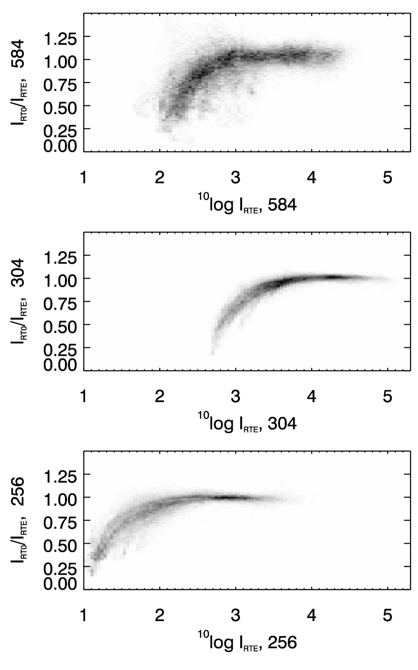
Figure 9: Joint probabilty distributions of the ratio $R_{\mathrm{CI}}=I_{\mathrm{RT0}}/I_{\mathrm{RTE}}$ as a function of $I_{\mathrm{RTE}}$. Tops to bottom panels show the relations for He I $\lambda 584$, He II $\lambda 304$, and He II $\lambda 256$.

Table 5: Ratios of average line intensities illustrating the effect of coronal illumination.

Ratio	He i $\lambda$584	He ii $\lambda$304	He ii $\lambda$256
$R_{\mathrm{CI}}$	1.01	0.98	0.97

Next we assess the effects of coronal illumination. To remove this effect, and this effect alone, we need to run a new Bifrost simulation including non-equilibrium ionisation but with the photoionisation switched off, and with a snapshot from this simulation calculate the NE-NLTE radiative transfer solution with the new ion fractions. This costs more than we can afford. Instead we compare the equilibrium line intensities, $I_{\mathrm{RTE}}$, with non-LTE line intensities, $I_{\mathrm{RT0}}$. The former includes the effect of coronal illumination, the latter does not.

Table 5 gives the ratio

$$R_{\mathrm{CI}}=\frac{\langle I_{\mathrm{RT0}}\rangle}{\langle I_{\mathrm{RTE}}\rangle}$$ (19)

for the three resonance lines. The value is approximately one for all of them. This suggests that the effect of coronal illumination is negligible for the mean quantities. Andretta & Jones (1997) found that the effect of an incident EUV radiation field influenced the line intensity of He I $\lambda 584$ only for their models featuring a low density transition region. Their models with a high density transition region had a low sensitivity to the coronal illumination. The high intensity network regions in our model correspond to the high density transition region models of Andretta & Jones (1997). These regions dominate in the line intensity averages, and this explains why the values of $R_{\mathrm{CI}}$ are approximately equal to one. To verify this explanation we visualise the effect of coronal illumination for all columns of our model in Figure 9, which shows the distribution of $I_{\mathrm{RT0}}/I_{\mathrm{RTE}}$ as a function of $I_{\mathrm{RTE}}$. For the He I $\lambda 584$ line the ratio is lower than one in low intensity regions and approximately one in high intensity regions. This is the trend also for the He II $\lambda 304$ and He II $\lambda 256$ lines showing that the effect of the coronal illumination is more important in low intensity regions.

7 Discussion

Figure 10: Average line profiles based on the NE-NLTE intensity of the whole model atmosphere.

Suggestions on various enhancement mechanisms have been made in the past. Particle diffusion (Fontenla et al., 1993) and velocity redistribution (Andretta et al., 2000) are examples that would both lead to a mixing of hot electrons and cold ions. Presence of a macroscopic velocity field across the transition region will have a qualitatively similar effect, as was shown by Fontenla et al. (2002) in static 1D models. Our model atmosphere and radiative transfer calculations take time dependent 3D flows and non-equilibrium ionization into account, and we end up with another scenario of hot electrons exciting cold atoms (shown in Fig. 8). While we will not rule out possible effects due to particle diffusion and velocity redistribution, we can safely say that non-equilibrium effects enhance the intensities.

The calculated intensities are dependent on the ionization state, and the ionization state is dependent on the 3D structure and 3D radiation of the atmosphere. Modelling the radiation field in 1D will potentially lead to erroneous ion fractions and therefore erroneous intensities. For instance, a chromospheric structure may be exposed to EUV radiation from the sides as well as from the top. Modelling the the radiation in 1D would expose such a structure to EUV radiation only from the top which would result in a lower photoionization rate and fewer ions. An example of this is given in Figure 7 of Leenaarts et al. (2016) where a comparison between 1D and 3D radiative transfer shows that an exposed chromospheric structure has a higher number density of He II in the 3D case than in the 1D case.

Another enhancement mechanism that has been suggested is the PR-mechanism. We have shown that a significant amount of the He i $\lambda$584 photons are created in recombination cascades. This is valid in both network and internetwork regions of our model. According to Milkey (1975) the PR-mechanism should lead to a central reversal in the line profile. Figure 10 shows the average profiles of all three of the studied resonance lines, where the intensity is from NE-NLTE radiative transfer calculation. The He I $\lambda 584$ profile clearly has a central reversal, even after averaging over all the columns. We found that the coronal illumination is important for the 584 line intensity in the low-intensity internetwork regions, but less so in the high intensity network regions. The column shown in Figure 6 is from such a high intensity network column, and the figure shows the effect of recombination cascades. This suggests that the photoionisation in the network is dominated by internal sources of EUV photons - not an externally set coronal illumination. The possible internal sources of photons capable of ionising He i included in the calculations are He II $\lambda 304$, He II $\lambda 256$, and the two helium continua. Also photons from the hydrogen Lyman continuum shortward of 504 Å are capable of ionising He i. The hydrogen Lyman continuum is included as a background element, and the contribution is determined by the non-equilibrium hydrogen populations from the Bifrost simulation. An investigation of the relative importance of these internal photon sources is beyond the scope of the present study.

These findings are consistent with Andretta & Jones (1997), who found that the resonance line of neutral helium has a low sensitivity to coronal illumination in models with a high density transition region. The question is then: have He I $\lambda 584$ central reversals been observed? A central reversal was measured by Phillips et al. (1982). Wilhelm et al. (1997) reported single peaked average profiles based on observations from SOHO/SUMER (Wilhelm et al., 1995). Later both Peter (1999) and Judge & Pietarila (2004) found indications of central reversals, also based on observations from SOHO/SUMER. The line was also observed with SOHO/CDS (Harrison et al., 1995), but since the CDS instrument response function is broad, any double-peaked He I $\lambda 584$ profiles would have been washed out as was shown by Mauas et al. (2005). Our results can be brought into doubt if central reversals are uncommon features for the He I $\lambda 584$ profile. They have been observed, but not everywhere. However, the observation of narrow double-peaked profiles may have been prevented by a too low spectral resolution of the relevant instruments. We believe therefore that the central reversal present in our modelled He I $\lambda 584$ profiles is not in conflict with observations. However, further studies on this issue are merited.

We found that the resonance lines of He ii are primarily excited by collisions. The role of PR is moderate for He II $\lambda 304$ and marginal for He II $\lambda 256$. This is also reflected in the average profiles shown in figure 10: the He II $\lambda 304$ profile has a slightly flattened peak and the He II $\lambda 256$ profile appears Gaussian. Our finding that the He ii lines are collisionnally excited in the quiet sun is in agreement with what has been concluded in earlier studies (Jordan et al., 1993; Andretta et al., 2003; Jordan & Brosius, 2007).

8 Summary and conclusion

We use the code Multi3d to solve the radiation transfer problem for helium on a radiation-MHD simulation snapshot. By constraining the radiative transfer solution with the non-equilibrium helium ion fractions, we are able to obtain non-equilibrium non-LTE atomic spectra. The EUV resonance lines He I $\lambda 584$, He II $\lambda 304$, and He II $\lambda 256$ have intensities an order of magnitude higher than what we get by assuming optically thin equilibrium conditions. This difference is in line with the difference between observed and modelled intensities reported in the literature.

The high NE-NLTE intensity of He I $\lambda 584$ is explained by large contributions from recombination cascades. The high NE-NLTE intensity of He II $\lambda 304$ and He II $\lambda 256$ is explained primarily by non-equilibrium effects. A higher number of He II ions are present in the high temperature transition region that what is permitted under equilibrium conditions. The collisional excitation rates of the He II line transitions are increasing with temperature. Thus there is more collisional excitation and more photons are produced in the lines when non-equilibrium ionisation is taken into account.

We conclude that the problem of the anomalously high helium EUV line intensities disappears when taking into account optically thick radiative transfer and non-equilibrium ionisation effects.