Chaos and correlated avalanches
in excitatory neural networks with synaptic plasticity

Abstract

A collective chaotic phase with power law scaling of activity events is observed in a disordered mean field network of purely excitatory leaky integrate-and-fire neurons with short-term synaptic plasticity. The dynamical phase diagram exhibits two transitions from quasi-synchronous and asynchronous regimes to the nontrivial, collective, bursty regime with avalanches. In the homogeneous case without disorder, the system synchronizes and the bursty behavior is reflected into a period doubling transition to chaos for a two dimensional discrete map. Numerical simulations show that the bursty chaotic phase with avalanches exhibits a spontaneous emergence of persistent time correlations and enhanced Kolmogorov complexity. Our analysis reveals a mechanism for the generation of irregular avalanches that emerges from the combination of disorder and deterministic underlying chaotic dynamics.

Networks of spiking neurons feature a wide range of dynamical collective behaviors, that are believed to be crucial for brain functioning Vogels et al. (2005). Next to uncorrelated and asynchronous dynamics, quasi-synchronous phases and regimes of irregular activity have been observed, showing a still unexplained degree of correlation that could encode part of the neural function Hulata et al. (2005); Shu et al. (2003); Wang (2010); Destexhe et al. (2007); Hesse and Gross (2014); Sanchez-Vives and McCormick (2000). Understanding the mechanisms that generate such experimentally observed collective behaviors and the transition between them is a major goal in theoretical neuroscience Vogels et al. (2005); Abbott and van Vreeswijk (1993); van Vreeswijk (1996); Kadmon and Sompolinsky (2015); Brunel (2000); Kirst et al. (2009); Montbrió et al. (2015); Hansel and Mato (2003); Panzeri et al. (2001). A particularly interesting dynamical signature of collective irregular regimes are avalanches or bursts of spiking neurons with heavy-tailed distributions of activity Hesse and Gross (2014); Mejias et al. (2010); Livi (2013). Interestingly, in cortical networks, irregular activity at the collective level Burns and Webb (1976); London et al. (2010) and avalanches characterized by power law distributions have been widely observed both in vitro and in vivo Beggs and Plenz (2003); Segev et al. (2001); Petermann et al. (2009); El Boustani et al. (2009). These regimes are thought to be closely related to information processing in the cortex Kinouchi and Copelli (2006); Ostojic (2014); Monteforte and Wolf (2012) and to adaptive Chialvo (2010) and healthy Massobrio et al. (2015) behavior.

Several mechanisms leading to irregular dynamics and bursts in networks of spiking neurons have been proposed. Irregular dynamical phases have been related to a balance between excitatory and inhibitory inputs Amit and Brunel (1997); van Vreeswijk and Sompolinsky (1996) or to a disorder in the network or in the couplings Brunel (2000); Cortes et al. (2013) as crucial ingredients. Power law distributed avalanches have been attributed to synaptic plasticity with a stochastic noise in the charging Levina et al. (2007); Bonachela and Muñoz (2009); Bonachela et al. (2010); Millman et al. (2010); Volman et al. (2004) or to dynamical mechanisms inspired by self organized criticality (SOC) de Arcangelis et al. (2006); Chialvo (2010); di Santo et al. (2016). The balance between excitation and inhibition plays an important role in the latter dynamical regime as well Lombardi et al. (2012), and a relation between uncorrelated dynamics in a network of stochastic units and power law scaling has been proposed Touboul and Destexhe (2010, ).

In this Letter we show that correlated irregular dynamics can be observed in homogeneous deterministic networks of $N$ identical purely excitatory spiking neurons endowed with synaptic plasticity, coupled by an all to all, mean field (MF), interaction. In this case, all neurons are synchronized but, for small enough synaptic decay time, the system displays a period doubling transition from a periodic phase to synchronous chaos ding et al. (1980); heagy . Such a transition is determined by the competition among the system time scales in the strong and weak coupling limits. For vanishing synaptic decay time, the dynamics can be reduced to a one dimensional map.

In the presence of disorder in the couplings, we show that the dynamics exhibits three phases, depending on the interaction strength and synaptic decay time. In particular, next to the quasi-synchronous and the asynchronous regimes Burioni et al. (2014), a phase characterized by power law distributed avalanches emerges in correspondence to the chaotic phase of the homogeneous MF model. Chaos is preserved in this dynamical phase, as confirmed by the computation of the Lyapunov exponents, and it is characterized by the onset of strong temporal correlations and high complexity. Our analysis uncovers a connection between dynamical stability and emergent avalanche activity in the presence of short-term synaptic plasticity, that may go beyond our particular case of study.

We consider a disordered random network of leaky integrate-and-fire (LIF) neurons Izhikevich (2004) connected via the Tsodyks-Uziel-Markram (TUM) model for short term synaptic plasticity Tsodyks et al. (2000). Within a Degree based Mean Field approximation (DMF), for each neuron $i=1\dots N$ the dynamics is defined by three differential equations:

$$\dot{v}_{i}(t) = a-v_{i}(t)+gk_{i}Y(t)$$ (1)

$$\dot{y}_{i}(t) = -\frac{y_{i}(t)}{\tau_{in}}+u(1-y_{i}(t)-z_{i}(t))S_{i}(t)$$ (2)

$$\dot{z}_{i}(t) = \frac{y_{i}(t)}{\tau_{in}}-\frac{z_{i}(t)}{\tau_{R}},$$ (3)

where $v_{i}(t)$ is the membrane potential of neuron $i$ while $y_{i}(t)$, $z_{i}(t)$ and $x_{i}(t)=1-y_{i}(t)-z_{i}(t)$ represent the active, inactive and available fraction of resources of the corresponding synapses. The potential $v_{i}(t)$ is reset to $0$ at times $t_{i}(m)$ when it reaches the threshold $v_{i}(t_{i}(m))=1$. At $t_{i}(m)$, a spike activates a fraction $u$ of the available resources, and the activation is modeled as a spike train $S_{i}(t)=\sum_{m}\delta(t-t_{i}(m))$. Neurons are characterized by the coupling constant $gk_{i}$, randomly extracted from the distribution $P(k_{i})$. $Nk_{i}$ can be interpreted as the effective number of neural synapses interacting with neuron $i$, i.e its in-degree Burioni et al. (2014). In this framework, $k_{i}$ is the only relevant topological feature of the neural network and it justifies the DMF name. In a mean field description, the incoming synaptic current can be written as the average of the active resources $Y(t)=N^{-1}\sum_{i=1}^{N}y_{i}(t)$.

By introducing an event driven map Brette (2007), the DMF approach allows for very effective numerical simulations and it has been shown to reproduce the relevant collective dynamics for networks with large finite connectivity and metrical features di Volo et al. (2014) (see Supplemental Material (SM) supp ).

Eqs. (1-3) are characterized by three time scales: the period of the oscillating non interacting neuron $T=\log(a/(a-1))$, the recovery time $\tau_{R}$ and the synaptic decay time $\tau_{in}$. The regime $\tau_{in}\lesssim T$ has been studied in detail in Burioni et al. (2014); di Volo et al. (2014, 2013); PhysRevE.90.042918 , and it features a transition from a quasi-synchronous to an asynchronous phase as a function of $g$ and of the shape of $P(k_{i})$. Here we will focus instead on the regime $\tau_{in}\ll T\ll\tau_{R}$, setting $a=1.3$, $\tau_{R}=10$ and varying $\tau_{in}$ between $10^{-1}$ and $10^{-5}$. These parameters are consistent with those selected in Tsodyks et al. (2000), where they have been chosen on the basis of biological motivations.

Mean Field. The presence of a further non trivial phase can be put into evidence by considering the simple in-degree distribution $P(k_{i})=\delta(k_{i}-k_{0})$. In this fully MF case, where all the coupling constants are equal, all neurons become completely synchronized after an initial transient state, as shown in the SM. Hence, Eqs. (1-3) reduce to the equations of a single neuron with coupling $k_{0}$ and $Y(t)=y(t).$ The dynamics can be rewritten as an event driven Poincaré map in $z_{n}$ and $y_{n}$, representing the inactive and active resources before the $n$-th synchronous spiking event (see SM):

$$y_{n+1} = e^{-\frac{\Delta_{n}}{\tau_{in}}}(y_{n}+u(1-y_{n}-z_{n}))$$ (4)

$$z_{n+1} = -e^{-\frac{\Delta_{n}}{\tau_{in}}}\frac{y_{n}+u(1-y_{n}-z_{n})}{1-\tau_{in}/\tau_{R}}$$ (5)

$$+e^{-\frac{\Delta_{n}}{\tau_{R}}}\left(z_{n}+\frac{y_{n}+u(1-y_{n}-z_{n})}{1-\tau_{in}/\tau_{R}}\right),$$

where the time interval $\Delta_{n}$ between the $n$-th and the ($n+1$)-th spiking event is obtained from:

$$1 = a-e^{-\frac{\Delta_{n}}{\tau_{in}}}\frac{g\tau_{in}k_{0}(y_{n}+u(1-y_{n}-z_{n}))}{1-\tau_{in}}$$

$$-e^{-\Delta_{n}}\left(a-\frac{g\tau_{in}k_{0}(y_{n}+u(1-y_{n}-z_{n}))}{1-\tau_{in}}\right).$$

When $\tau_{in}\ll T\ll\tau_{R}$, an insight on the dynamics can be achieved by considering the opposite regimes of weak and strong interaction, i.e. when $gk_{0}Y(t)$ or $a-v_{k_{0}}(t)$ are negligible in Eq. (1), respectively. In both extreme regimes, the map in Eqs. (4-Chaos and correlated avalanches in excitatory neural networks with synaptic plasticity) can be solved, and it features a fixed point corresponding to a periodic solution in the continuous dynamics (see SM for details). In particular, in the weak coupling regime, the periodicity is trivially $T$, and the interaction term remains negligible if $gk_{0}\tau_{in}\ll\tau_{R}/T$. On the other hand, if the $a-v_{k_{0}}(t)$ term can be ignored, the system displays a much faster periodicity: $T_{f}=\tau_{R}/(gk_{0}\tau_{in})$ and the approximations holds only if $gk_{0}\tau_{in}\gg\tau_{R}/\tau_{in}$.

If $\tau_{R}/T\ll gk_{0}\tau_{in}\ll\tau_{R}/\tau_{in}$, neither the weak nor the strong coupling conditions are satisfied, and the competition between the terms with a slow and a fast dynamics plays a non trivial role, destroying the presence of a periodic evolution. Such a behavior can be analyzed by means of the bifurcation diagram ott of $\Delta_{n}$ as a function of $g$ at fixed $\tau_{in}$. Fig. 1 shows the presence of a stable fixed point for small and large values of $g$, describing a slow and a fast periodic regime, respectively. For an intermediate value, a period doubling appears first; then, at $g>g^{\prime}(\tau_{in})$, the distribution of $\Delta_{n}$ becomes continuous. The $\Delta_{n}$ becomes again delta-distributed for $g>g^{\prime\prime}(\tau_{in})$. In the SM we show that for $g^{\prime}(\tau_{in})<g<g^{\prime\prime}(\tau_{in})$ the maximum Lyapunov exponent Benettin et al. (1980) becomes positive, a signature of the presence of chaos. In the fully MF system with $N$ neurons, this is an example of synchronous chaos ding et al. (1980); heagy . The phase diagram in Fig. 2 shows that the $\tau_{in}$-dependence of the boundaries of the chaotic phase (squares) is consistent with the continuous lines, obtained by the weak and strong coupling limit arguments. The critical values for $g$ and $\tau_{in}$ depend on $a$, i.e. the intrinsic period of the neuron; the chaotic dynamics is observed at higher $\tau_{in}$ by considering smaller $a$ (see SM). Taking the limit $\tau_{in}\to 0$ with $g_{\rm eff}=gk_{0}\tau_{in}$ constant in Eqs. (4-Chaos and correlated avalanches in excitatory neural networks with synaptic plasticity), one obtains a single variable map as a function of $g_{\rm eff}$, $a$ and $\tau_{R}$ only, that can be studied analytically (see SM). This simpler map confirms the presence of a genuine chaotic dynamical phase.

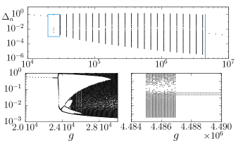
Figure 1: Feigenbaum bifurcation diagram for the MF TUM model in Eqs. (4-5) with $\tau_{in}=10^{-3}$. The attractor for the interspike interval of the network $\Delta_{n}$ is showed as a function of the coupling $g$. Upper panel: bifurcation diagram in the full relevant range of the parameter $g$. Lower-left panel: magnification on the period doubling cascade at the first transition. Lower-right panel: magnification on the second transition. The blue rectangles in the upper panel indicate the zooming regions of the lower panels.

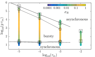
Figure 2: (Color online) Dynamical phase diagram of the MF and DMF models in terms of the coupling constants $g$ and of the synaptic time scale $\tau_{\rm in}$. MF model: The squares indicate the $g$ values at which the transition to chaos (along with the discontinuity of the interspike time standard deviation) takes place (see SM). The black lines are linear fits. DMF model: Each colored point corresponds to a simulation, the color code indicating $\sigma_{R}$ at the corresponding value of $(g,\tau_{\rm in})$. The intervals of $g$ containing the discontinuity (c.f. Fig. 3) are signaled with black circles.

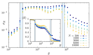
Figure 3: (Color online) Standard deviation of the Kuramoto parameter, $\sigma_{R}$ versus $g$ for the DMF model with $\tau_{in}=10^{-3}$ and five values of $N$. In the quasi-synchronous and bursty phases the data corresponding to the two larger values of $N$ overlap within their statistical errors, indicating convergence in size, while deep in the asynchronous phase they decrease as $\sim N^{-1/2}$. Inset: temporal average of $R(t)$, showing that the larger sizes have attained their asymptotic value in all the phases. The vertical stripes are common to all the figures in the article and indicate the apparent discontinuity of $\langle R\rangle$ for the largest sizes.

Degree based Mean Field. Let us now focus on the multi-site DMF model with heterogeneous couplings extracted from the distribution $P(k_{i})$. We consider a Gaussian $P(k_{i})$ with average $\mu=0.7$ and standard deviation $\sigma=0.077$, although our results are robust for different distributions (see SM for a discussion). A relevant quantity describing the level of synchronization of the neurons is the Kuramoto parameter Acebrón et al. (2005): $R\left(t\right)=\frac{1}{N}\left|\sum_{i=1}^{N}\textrm{e}^{\imath\phi_{i}\left(t\right)}\right|$ where $\phi_{i}(t)$ is the phase of neuron $i$ at time $t$:

$$\phi_{i}(t)=2\pi\frac{t-t_{i}(m)}{t_{i}(m+1)-t_{i}(m)},$$ (7)

where $t_{i}(m)$ is the $m$-th spike of neuron $i$ and $t\in[t_{i}(m),\,t_{i}(m+1)]$. In Fig. 3 the time average $\langle R\rangle$ of the Kuramoto parameter and its fluctuations $\sigma_{R}$ are displayed as a function of $g$. At small couplings, $\langle R\rangle\approx 1$ and the fluctuations are small, as the systems is in a quasi-synchronous phase. At large $g$, $\langle R\rangle$ becomes very small ($\langle R\rangle\rightarrow 0$ with increasing $N$), consistently with a periodic asynchronous phase. In the irregular, bursty, regime, $\langle R\rangle$ exhibits moderate values and, more significantly, its fluctuations grow abruptly by an order of magnitude; this is a signal of a complex dynamical phase, illustrated in the raster plot in the inset of Fig. 4 (each dot corresponds to a spike of neuron $i$ at time $t$). The fluctuations of $\langle R\rangle$ originate from the alternations of synchronous events with asynchronous phases characterized by smaller bursts where only a subset of the neurons fires simultaneously. The main plot of Fig. 4 shows that the size $s$ of such bursts, or avalanches, is broadly distributed (see SM for a detailed definition of burst size). Interestingly, the distribution is compatible with a power law $h(s)\sim s^{-\gamma}$ followed by a bump. The power $\gamma$, close to $2$ (see SM), does not depend significantly on $N$, nor on $g$ for a wide $g$-range in the bursty phase. Finally, the peaks at large $s$ in the distributions correspond to synchronous events where all neurons fire quasi-simultaneously, and their position scales with the system size.

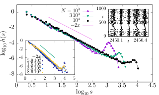
Figure 4: (Color online) Avalanche size histogram $h(s)$ of the DMF model, $\tau_{in}=10^{-3}$ and $g=3.5\cdot 10^{5}$ in the bursty regime, for several values of $N$. Upper inset: a fragment of the raster plot for the same system. Lower inset: $\log_{10}h(s)$ for $N=10^{4}$ and various values of $g$ across the bursty phase.

The natural issue is the relation between the chaotic phase in the single site MF model and the bursty-avalanche regime of the multi-site DMF approach. In the SM we show that also the bursty phase is characterized by a chaotic dynamics with positive Lyapunov exponents. In Fig. 2 we have superimposed the dynamical phase diagrams of the MF and DMF models. In the DMF, the transitions points (circles) are set at the $g$ intervals at which the abrupt increments of the fluctuations of the Kuramoto parameter take place (c.f. Fig. 3). In the MF case, the squares indicate the values of $g$ at which the transitions to chaos occur. While the phase diagrams slightly differ, the phase diagram of the DMF model converges continuously to that of the MF model in the limit of vanishing width of the distribution $P(k_{i})$, as illustrated in the SM. This scenario suggests that the bursty regime arises from the introduction of disorder on a system with synchronous chaos, so that neurons with different coupling $k_{i}$ do not fire simultaneously and the synchronous solution loses stability.

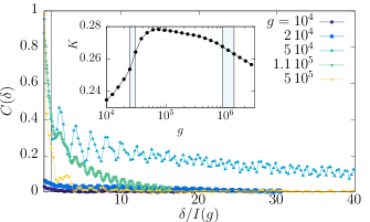
Figure 5: (Color online) Main plot: connected correlation function $C$ as a function of the time difference $\delta$ in units of the average interspike time $I(g)$, for several values of $g$ in the DMF model with $\tau_{in}=10^{-3}$, $N=800$. For values of $g$ in the bursty phase, the correlation remains high even after large time differences. Inset: Kolmogorov Complexity of the DMF model, $\tau_{in}=10^{-3}$, $N=10^{3}$, and the spike time differences $\Delta_{n}$ stored with 14 digits of precision.

In the DMF model, the transition to the bursty collective behavior also corresponds to the presence of large temporal correlations. We define the time dependent complex correlation, $c(\delta,t)=(1/N)\sum_{i=1}^{N}{e^{\imath\phi_{i}(t)}e^{-\imath\phi_{i}(t+\delta)}}$, where $\phi_{i}(t)$ is the Kuramoto phase (7), along with the connected correlation function, $C(\delta)=|\langle c(\delta,t)\rangle_{t}|-|\langle c({\cal T},t)\rangle_{t}|$, as the temporal average $\langle\cdot\rangle_{t}$ of $c$ over a sufficiently large interval of times $t$, minus its stationary value at a sufficiently large time difference, $\delta={\cal T}$ (for details at this regard see the SM section). $C(\delta)$ measures in this way the average amount of correlation between spike configurations separated by a time delay $\delta$. The quantity $C(\delta)$ (see Fig. 5, main panel) reveals the existence of large correlations for times $\delta$ much larger than the average interspike time, $I(g)$, only in the bursty regime (for $3\cdot 10^{4}\lesssim g\lesssim 10^{5}$ at $\tau_{in}=10^{-3}$), while in the synchronous and asynchronous regimes, $C(\delta)$ decays faster to its asymptotic value.

Another interesting quantity in temporal series of neural firing patterns is the amount of information they can sustain. In information theory, the Kolmogorov Complexity (KC) of a data sequence determines the length of the minimum computer program generating it, hence being a measure of the sequence predictability Li and Vitányi (1993). KC has been related to the computational power of artificial neural networks Balcazar et al. (1997), and used in the quantitative characterization of epileptic EEG recordings Petrosian (1995). We consider the KC of the raster plot, interpreting it as an estimation of the amount of information that can be codified in the dynamical signal (see the details of the KC estimation in the SM section). The numerical results for the DMF model reveal that the KC as a function of $g$ (see the inset of Fig. 5) presents a maximum in the bursty regime (around $g\simeq 6\,10^{4}$ for ${\tau_{in}=10^{-3}}$).

In summary, we have reported the existence of a dynamical phase occurring in a network of purely excitatory LIF neurons connected with synaptic plasticity. This phase, identified by average statistical properties of the Kuramoto parameter, is strongly chaotic and it differs from previously known irregular phases for similar models, e.g. phases with chaotic transient dynamics Cortes et al. (2013); Zillmer et al. (2006). The chaotic phase must also be distinguished from previous irregular regimes observed in spiking neural models, namely weak chaos in purely excitatory disordered networks Olmi et al. (2010) or stable chaos in inhibitory ones Zillmer et al. (2009); Ullner and Politi (2016); Pazó and Montbrió (2016). The emergent dynamical regime occurs in a large region of the phase diagram, and it is separated by two dynamical transitions from the quasi-synchronous and asynchronous regimes. Chaos is preserved in the presence of disordered couplings. In that case, interestingly, the chaotic phase also features characteristic power law distributed avalanches. By properly defining temporal correlations and tools from information theory, we show that the additional bursty phase is strongly correlated and it carries a relevant amount of information compared to the quasi-synchronous and the asynchronous phases.

in 1,…,26