Positivity for convective semi-discretizations

Abstract

We propose a technique for investigating stability properties like positivity and forward invariance of an interval for method-of-lines discretizations, and apply the technique to study positivity preservation for a class of TVD semi-discretizations of 1D scalar hyperbolic conservation laws. This technique is a generalization of the approach suggested in [12]. We give more relaxed conditions on the time-step for positivity preservation for slope-limited semi-discretizations integrated in time with explicit Runge–Kutta methods. We show that the step-size restrictions derived are sharp in a certain sense, and that many higher-order explicit Runge–Kutta methods, including the classical 4th-order method and all non-confluent methods with a negative Butcher coefficient, cannot generally maintain positivity for these semi-discretizations under any positive step size. We also apply the proposed technique to centered finite difference discretizations of scalar hyperbolic and parabolic problems.

1 Introduction

A number of important PDE models have the property that they preserve positivity of the initial data:

$$U(x,t_{0}) \geq 0\implies U(x,t)\geq 0 \forall\ \ t\geq t_{0},$$ (1)

or (more strongly) that they preserve the interval containing the initial data:

$$U_{\text{min}}\leq U(x,t_{0}) \leq U_{\text{max}}\implies U_{\text{min}}\leq U(x,t)\leq U_{\text{max}} \forall\ \ t\geq t_{0}.$$ (2)

Examples of such PDEs include scalar hyperbolic conservation laws in one spatial dimension, as well as the heat equation and some of its generalizations. In this work we study a technique that was first used in [12, 13] for determining whether a certain class of numerical discretizations satisfies the discrete analog of (1) or (2).

We focus on the application of this technique to the initial-boundary-value problem given by the hyperbolic conservation law (6) below, together with positive initial and boundary data. A common approach to solving hyperbolic conservation laws numerically is to discretize in space with a slope or flux limiter, and in time with an explicit Runge–Kutta (explicit RK, or ERK) method. It is natural to ask whether the positivity property is retained under this discretization. This question is usually analyzed by using Harten’s theorem [7, Lemma 2.2] to show positivity under explicit Euler integration, and then applying a higher-order strong stability preserving (SSP) method in time [6]. This can be thought of as a method-of-lines positivity analysis, in which the spatial and temporal discretizations are analyzed separately. In the present work, we perform a direct positivity analysis of fully discretized schemes, obtaining stronger results than what can be achieved by considering only Harten’s theorem and SSP methods. These results provide a theoretical basis for some empirical observations in [9, 11], wherein various Runge–Kutta integrators preserved strong stability properties under step sizes much larger than those suggested by the existing theory.

Following the usual terminology, the term positivity in the context of positivity preservation is always meant herein in the weak sense; i.e., it means non-negativity. Although we focus on positivity to simplify the presentation, the conditions we derive are necessary and sufficient for forward invariance of an interval; see Theorem 1.

Our paper is organized as follows. In Section 1.1, we review a widely-used class of total-variation-diminishing (TVD) semi-discretizations for hyperbolic conservation laws (6), resulting in a system of ODEs with a specific structure. In Section 2, we introduce the concept of (positivity) step-size coefficient, and present our main theoretical results, showing sufficient or necessary conditions for positivity preservation for this system of ODEs when integrated with an explicit Runge–Kutta method. In the rest of the paper we investigate the step-size coefficients in some classes of ERK methods. In Section 3, we summarize the results of [12] on the optimal SSP coefficient and positivity step-size coefficient for two-stage, second-order ERK methods. In Section 4, we present our main computational results for three-stage, third-order ERK methods. We determine the optimal step-size coefficient in each of the three subclasses: methods with optimal step-size coefficient are essentially characterized in the two-parameter subclass, whereas optimal methods in the two, one-parameter subclasses are completely described. We also discover that the unique three-stage, third-order ERK method having the minimum truncation-error coefficient also belongs to the set of methods with maximum step-size coefficient. In the proofs we are to find certain maximal hypercubes over which some multivariable polynomials are simultaneously non-negative. Section 5 extends our analysis to higher-order ERK methods with more stages, and shows many negative results. Throughout Sections 3-5, the ERK methods have been applied to the upwind semi-discretization of the advection equation. In Section 6, we illustrate the applicability of the proposed ideas to the centered spatial discretization of the advection equation and to the heat equation. Finally, in Appendix A we present some Mathematica code to generate the multivariable polynomials corresponding to an ERK method, and test their non-negativity in hypercubes.

1.1 TVD semi-discretizations under Runge–Kutta integration

Semi-discretizations with a slope limiter can be analyzed as follows [10, Chapter III, Section 1.1-1.3]—below $U$ will denote the PDE solution, while the corresponding lower-case letter is used in semi-discretized ODEs. For concreteness we first consider the advection equation

$$U_{t}+a(t)U_{x} =0$$ (3)

with $a>0$; the following analysis can be extended to arbitrary variations in $a$. We discretize in space by

$$u^{\prime}_{k}(t)=\frac{1}{\Delta x}\left(f_{k-\frac{1}{2}}-f_{k+\frac{1}{2}}\right),$$ (4)

where $\Delta x$ is the spatial mesh width, and the fluxes are given by

$$f_{k+\frac{1}{2}}:=a(t)\left(u_{k}+\psi(\theta_{k})\left(u_{k+1}-u_{k}\right)\right).$$

Here $\psi$ is known as the limiter function and $\theta_{k}$ is a ratio of divided differences. This discretization leads to the form

$$u_{k}^{\prime}(t)=\frac{a(t)}{\Delta x}\left(1-\psi(\theta_{k-1})+\frac{1}{\theta_{k}}\psi(\theta_{k})\right)(u_{k-1}(t)-u_{k}(t)).$$ (5)

More generally, we consider the scalar nonlinear conservation law

$$U_{t}+f(U)_{x} =0,$$ (6)

where for simplicity we assume $f^{\prime}\geq 0$. The flux-differencing semi-discretization (4) is again used, with the flux now given by $f_{k+\frac{1}{2}}:=f(u_{k+\frac{1}{2}})$ where

$$u_{k+\frac{1}{2}}:=u_{k}+\psi(\theta_{k})(u_{k+1}-u_{k}).$$ (7)

By using the mean-value theorem, this can be written as

$$u_{k}^{\prime}(t)=\frac{f^{\prime}(\eta_{k})}{\Delta x}\left(1-\psi(\theta_{k-1})+\frac{1}{\theta_{k}}\psi(\theta_{k})\right)(u_{k-1}(t)-u_{k}(t)),$$

for some $\eta_{k}\in[u_{k-\frac{1}{2}},u_{k+\frac{1}{2}}]$.

It can be proved that non-negativity of (4) is ensured in either case if

$$1-\psi(\theta)+\frac{1}{\tilde{\theta}}\psi(\tilde{\theta})\geq 0$$ (8)

for all $\theta\in\mathbb{R}$ and $\tilde{\theta}\in\mathbb{R}\setminus\{0\}$. A sufficient condition for (8) is that

$$0\leq\psi(\theta)\leq 1\ \ (\theta\in\mathbb{R}),\quad\mathrm{and}\quad 0\leq\frac{1}{\theta}\psi(\theta)\leq\mu\ \ (\theta\in\mathbb{R}\setminus\{0\})$$ (9)

for some value of $\mu$. The upper bound $\mu$ will be important below when we discretize in time. Some well-known limiters satisfying conditions (9) include

• the minmod limiter [17], with $\psi(\theta)=\max\left(0,\min\left(1,\theta\right)\right)$ and $\mu=1$;

• the Koren limiter [14], with $\psi(\theta)=\max\left(0,\min\left(1,\frac{1}{3}+\frac{1}{6}\theta,\theta\right)\right)$ and $\mu=1$;

• the monotonized central limiter [19], with $\psi(\theta)=\max\left(0,\min\left(2\theta,\frac{1+\theta}{2},2\right)\right)$ and $\mu=2$.

In this work we do not deal with the influence of boundary conditions, so for simplicity we consider periodic boundaries. The initial-boundary-value problem corresponding to (4) can thus be written, with some suitable functions $q_{k}$, in the form

$$\begin{cases}u^{\prime}_{k}(t)\ =\displaystyle\ q_{k}(u(t),t)\ \frac{u_{k-1}(t)-u_{k}(t)}{\Delta x},&\quad k=1,\ldots,N,\\ u_{0}(\cdot)\ :=u_{N}(\cdot),&\\ u_{k}(t_{0}):=u_{k}^{0}&\quad k=1,\ldots,N.\\ \end{cases}$$ (10a)

We assume that the initial conditions are non-negative

$$u_{k}^{0}\geq\ 0, \quad k=1,\ldots,N$$ (10b)

and that (9) is satisfied, so that

$$0\leq q_{k}(v,t)\leq\lambda_{k}(\mu+1)$$ (10c)

holds for all $v,t$, with $\lambda_{k}:=\sup_{u\in[u_{k-\frac{1}{2}},u_{k+\frac{1}{2}}]}f^{\prime}(u)$. Under these assumptions, it can be shown that if the solution $u$ exists (which can be guaranteed, for instance, by assuming that $q_{k}$ is Lipschitz), then it is positive [12]: we have $u_{k}(t)\geq 0$ for $1\leq k\leq N$.

Suppose now that we discretize (10) in time with a given explicit Runge–Kutta method, and we want to preserve positivity. To achieve this, we aim to determine a value $\Delta t_{0}>0$ such that the RK solution and stage values are non-negative when applied to any problem of the form (10), under some step-size restriction $\Delta t\leq\Delta t_{0}$.

In the following examples we use the simplest RK method and give a suitable value for $\Delta t_{0}$.

Example 1 (Advection equation).

The forward Euler (FE) method preserves positivity for (10) whenever

$$\Delta t\leq\frac{\Delta x}{(\mu+1)\sup a(\cdot)}=:\tau_{0}.$$

In other words, if $v$ denotes the vector $(v_{1},\ldots,v_{N})$ and we set $v_{0}:=v_{N}$, then

$$v_{k}+\Delta t\cdot q_{k}(v,t)\ \frac{v_{k-1}-v_{k}}{\Delta x}\geq 0\ \text{for all}\ 0<\Delta t\leq\tau_{0},\ v\geq 0\textrm{ and }t\in[t_{0},T],$$

where $v\geq 0$ is understood componentwise.

Example 2 (Scalar conservation law).

The FE method preserves positivity for (10) whenever

$$\Delta t\leq\frac{\Delta x}{(\mu+1)\sup f^{\prime}(U(\cdot,t_{0}))}=:\tau_{0}.$$

Given an ERK method, it is natural to consider the factorization

$$\Delta t\leq\Delta t_{0}\equiv\gamma\tau_{0}$$ (11)

of the maximum allowed step size $\Delta t_{0}$, with $\tau_{0}$ appearing in Example 1 or 2, because (i) this product structure naturally arises during the computations (see (13)), and (ii) the factor $\gamma$, referred to as the (positivity) step-size coefficient, will depend only on the chosen ERK method, whereas $\tau_{0}$ depends on the right-hand side of the problem (10). We will sometimes write $\gamma(A,b)$, where $(A,b)$ refer to the Butcher coefficients of the RK method, to emphasize that the step-size coefficient depends on the method coefficients. Our general goal in this paper is to find the maximum value of $\gamma\geq 0$.

From (11) it is also apparent that $\gamma$ plays a role similar to that of the SSP coefficient of the RK method, denoted by ${\mathcal{C}}$, see [6]. Specifically, an RK method is guaranteed to preserve positivity for any positive system of ODEs with a general right-hand side $f(u(t),t)$, under the step-size restriction $\Delta t\leq{\mathcal{C}}\Delta t_{\textup{FE}}$, where $\Delta t_{\textup{FE}}$ is the positivity step-size threshold for the forward Euler method. We will see that, for many RK methods, $\gamma$ is strictly larger than the SSP coefficient, because in determining a value $\gamma$ we consider only problems of the form (10).

The present work is related to that presented in [8], in that it proves less restrictive step sizes for positivity of a particular class of problems. However, the class of problems considered herein is different from the class of problems considered there.

2 Positivity of the Runge–Kutta approximations

In this section we generalize and make systematic an approach that was introduced in [12, 13]. Applying an explicit RK method to (10) we obtain

$$y^{i}_{k}= u^{n}_{k}+\sum_{j=1}^{i-1}a_{ij}\xi_{k}^{j}\left(y^{j}_{k-1}-y^{j}_{k}\right),\quad k=1,\ldots,N,\ i=1,\ldots,m,$$ (12a)

$$u^{n+1}_{k}= u^{n}_{k}+\sum_{i=1}^{m}b_{i}\xi_{k}^{i}\left(y^{i}_{k-1}-y^{i}_{k}\right),\quad k=1,\ldots,N,$$ (12b)

where $u^{n}\approx u(t_{n})$, $t_{n}=n\Delta t$ and

$$\xi_{k}^{j}:=\frac{\Delta t}{\Delta x}q_{k}(y^{j},t_{n}+c_{j}\Delta t),\quad j=1,\ldots,m.$$ (13)

Here and throughout this work, superscripts on $y$, $u$ and $\xi$ denote indices rather than exponents. The coefficients $a_{ij}$ and $b_{j}$ can be conveniently represented by an $m\times m$ strictly lower-triangular matrix $A$ and an $m\times 1$ vector $b$, respectively (referred to as the Butcher tableau $(A,b)$).

The idea is to express each component of the stages and of the new solution as a combination of the previous solution values in the form

$$u^{n+1}_{k}=\sum_{i=0}^{m}P_{i}(\xi)u^{n}_{k-i},$$ (14)

where the functions $P_{i}$ are multivariable polynomials depending only on the method coefficients $(A,b)$, and $\xi$ is proportional to the time step size. These polynomials are independent of $k$ since the method is translation-invariant (though the values of $\xi$ do depend on $k$, in general). We then aim to compute the largest step size that ensures non-negativity of these polynomials.

Given a strictly lower-triangular matrix $A\in\mathbb{R}^{m\times m}$ and vector $b\in\mathbb{R}^{m}$, it can be shown (see Section 2.1) that the polynomials $P_{i}$ in (14) are multilinear functions of the variables $\xi^{j}_{\ell}$, and there are $m+1$ polynomials and $m(m+1)/2$ variables. Throughout this work we use the following ordering of the components of the vector $\xi$:

$$\xi=(\xi^{1}_{k-(m-1)},\xi^{1}_{k-(m-2)},\ldots,\xi^{1}_{k-1},\xi^{1}_{k};\xi^{2}_{k-(m-2)},\xi^{2}_{k-(m-3)},\ldots,\xi^{2}_{k-1},\xi^{2}_{k};\ldots;\xi^{m-1}_{k-1},\xi^{m-1}_{k};\xi^{m}_{k}).$$

2.1 Computation of the multivariable polynomials

The polynomials $P_{i}$ can be obtained directly from (12). To anticipate their structure, we rewrite (12) in matrix form. We begin by rewriting (12a) as

$$Y=e\otimes u^{n}+(A\otimes I_{N})Q_{mN}(I_{m}\otimes D_{N})Y,$$ (15)

where the vector $e:=(1,\ldots,1)\in\mathbb{R}^{m}$, $I$ is the identity matrix, the symbol $\otimes$ denotes the Kronecker product and subscripts denote the dimensions of each matrix. The matrix $D_{N}$ is the $N\times N$ cyclic tridiagonal matrix with entries $1,-1,0$ such that $[D_{N}]_{1,N}=1$, and $Q_{mN}$ is the $mN\times mN$ diagonal matrix with entries $\xi^{1}_{1},\xi^{1}_{2},\dots,\xi^{1}_{N},\dots,\dots,\xi^{m}_{N}$. Let

$$M:=(A\otimes I_{N})Q_{mN}(I_{m}\otimes D_{N}),$$

so that (15) becomes

$$Y=(I_{mN}-M)^{-1}(e\otimes u^{n}).$$

Since $A$ is now strictly lower-triangular, the matrix $M$ is strictly block lower-triangular, and we can write

$$Y=\sum_{i=0}^{\infty}M^{i}\left(e\otimes u^{n}\right)=\sum_{i=0}^{m-1}M^{i}\left(e\otimes u^{n}\right).$$

Thus (12b) becomes

$$u^{n+1}=\left(I_{N}+(b^{\top}\otimes I_{N})Q_{mN}(I_{m}\otimes D_{N})\sum_{i=0}^{m-1}M^{i}(e\otimes I_{N})\right)u^{n}.$$ (16)

Remark. By using the relation

$$M^{i}=(A\otimes I_{N})Q_{mN}\left((A\otimes D_{N})Q_{mN}\right)^{i-1}(I_{m}\otimes D_{N}),$$

we can also write (16) as

$$u^{n+1}=\left(I_{N}+(b^{\top}\otimes I_{N})Q_{mN}\sum_{i=0}^{m-1}\left((A\otimes D_{N})Q_{mN}\right)^{i}(e\otimes D_{N})\right)u^{n}.$$

2.2 A sufficient condition for non-negativity

In the present work we focus on positivity preservation, but—as we will see in Theorem 1 below—the step-size restrictions derived preserve a stronger property.

First notice that, by consistency, for any RK method we have

$$\sum_{i=0}^{m}P_{i}(\xi)=1.$$

Thus if $P_{i}(\xi)\geq 0$, then (14) shows that each solution value is a convex combination of solution values from the previous step. This motivates the following definition.

Definition 1.

Let an explicit Runge–Kutta method be given with coefficients $A,b$, and let $P_{i}$ denote polynomials defined implicitly by (14) when the method is applied to (10) and $\xi$ is defined by (13). The (positivity) step-size coefficient of the method is

$$\gamma(A,b):=\sup\{\delta\geq 0:P_{i}(\xi)\geq 0\textrm{ for each }0\leq i\leq m\textrm{ and all }\xi\in[0,\delta]^{m(m+1)/2}\}.$$

We sometimes write simply $\gamma$, omitting the dependence on the method coefficients when there is no potential for ambiguity. If the set appearing in the $\sup$ above is empty, we set $\gamma:=0$.

Geometrically, the step-size coefficient is the edge length of the largest hypercube in the non-negative orthant over which the polynomials $P_{i}$ are all non-negative.

From the above considerations it is clear that we have the following theorem.

Theorem 1.

Let an $m$-stage ERK method be given and let the polynomials $P_{0},\dots,P_{m}$ be such that application of the method to (10) yields (14). Suppose that the time and space step sizes are chosen so that

$$0\leq\Delta t\frac{q_{k}(u,t)}{\Delta x}\leq\gamma,\quad k=1,\ldots,N,$$ (17)

for all values $u,t$. Let $u_{\text{max}}=\max_{k}(u_{k}(t_{0}))$, $u_{\text{min}}=\min_{k}(u_{k}(t_{0}))$. Then the solution given by the Runge–Kutta method applied to (10) remains in the interval $[u_{\text{min}},u_{\text{max}}]$.

The invariance property appearing in Theorem 1—that is, preservation of the interval containing the initial data—is the discrete analog of a property known to hold for the exact solution of (6). As a special case, when $u_{\text{min}}\geq 0$ we have the property of positivity preservation.

2.3 Necessary conditions for non-negativity

Given a Runge–Kutta method $(A,b)$ and corresponding coefficient $\gamma(A,b)$, we may ask whether taking the step size larger than that permitted by (17) will always lead to negative solution values. The answer is “no”, but we can construct particular problems of the form (10) such that negative values will be obtained.

The following theorems apply to non-confluent methods. A Runge–Kutta method is said to be non-confluent if the stage approximations all correspond to distinct times; i.e., if there are no distinct $i,j$ such that $c_{i}=c_{j}$.

Theorem 2.

Let an explicit non-confluent Runge–Kutta method $(A,b)$ be given and let $\gamma(A,b)$ denote its step-size coefficient. Then for any $\tilde{\gamma}>\gamma$, there exists a problem (10), a function $q=q(t)$ and a step size satisfying

$$0<\Delta t\leq\tilde{\gamma}\frac{\Delta x}{\max_{k,t}q_{k}}$$

such that the prescribed method leads to a negative solution at the first step.

Proof.

By our assumptions, there exist $\tilde{\xi}\in[0,\tilde{\gamma}]^{m(m+1)/2}$ and an integer $j$ such that $P_{j}(\tilde{\xi})<0$.

Take $N=m$ and

$$u^{0}_{k}:=u_{k}(t_{0})=\begin{cases}1&\text{if }k=N-j\\ 0&\text{otherwise.}\end{cases}$$

Set $\Delta x=1$, $\Delta t=1$, and $q(\cdot,t_{0}+c_{j}\Delta t)=\tilde{\xi}^{j}$ for each $j$. Then direct computation reveals that $u_{N}^{1}=P_{j}(\tilde{\xi})u_{N-j}^{0}=P_{j}(\tilde{\xi})<0.$ ∎

Corollary 1.

Let an explicit non-confluent Runge–Kutta method be given. Then the time-step restriction (17) is sharp; i.e., it is the largest step size that guarantees positivity for all problems of the form (10).

The next result involves the concept of DJ-reducibility; see e.g. [3] for a definition. Note that any reducible method is equivalent to a method with fewer stages, so the irreducibility assumption here is no essential restriction.

Theorem 3.

Let an explicit non-confluent DJ-irreducible Runge–Kutta method $(A,b)$ be given such that at least one entry in the matrix $A$ or vector $b$ is negative. Then there exist initial data and a choice of $q$ such that the numerical solution of (10) obtained with the method includes a negative value. Therefore $\gamma(A,b)=0$.

Proof.

Let a RK method be given as in the theorem. We take initial data vector $v$ with $v_{p-1}=1$ where $p$ is an arbitrary grid index and $v_{k}=0$ for all $k\neq p-1$. To simplify the presentation, in this proof only we define $a_{m+1,j}:=b_{j}$ and $y_{m+1}:=u^{n+1}$. Let $i$ be the index of the first RK stage with a negative coefficient and suppose that $a_{iJ}<0$. We have

$$y^{i}_{p} =v_{p}+\sum_{j=1}^{m}a_{ij}q_{p}(y^{j},t_{0}+c_{j}\Delta t)\frac{\Delta t}{\Delta x}(y^{j}_{p-1}-y^{j}_{p}).$$

We let

$$q_{p}(u,t)=\begin{cases}0&t\neq t_{0}+c_{J}\Delta t\\ 1&t=t_{0}+c_{J}\Delta t,\end{cases}$$

so that

$$y^{i}_{p} =v_{p}+a_{iJ}\frac{\Delta t}{\Delta x}(y^{J}_{p-1}-y^{J}_{p}).$$

Furthermore, for all $j\leq J$ we have $y^{j}=v$; in particular, $y^{J}=v$. Thus

$$y^{i}_{p} =v_{p}+a_{iJ}\frac{\Delta t}{\Delta x}(v_{p-1}-v_{p})=a_{iJ}\frac{\Delta t}{\Delta x}<0.$$

If $i=m+1$ (i.e., if there is some $i$ such that $b_{i}<0$), then we are done.

Suppose to the contrary that $b_{j}\geq 0$ for all $j$. Suppose further that $b_{i}\neq 0$. Then by letting

$$q_{p+1}(u,t)=\begin{cases}0&t\neq t_{0}+c_{i}\Delta t\\ 1&t=t_{0}+c_{i}\Delta t,\end{cases}$$

we obtain

$$u^{n+1}_{p+1}=b_{i}\frac{\Delta t}{\Delta x}(y^{i}_{p}-y^{i}_{p+1})<0.$$

The last inequality follows by deducing from the construction above that $y^{i}_{p+1}=0$.

Finally, suppose that $b_{i}=0$, so that stage $i$ is not used directly to compute the new solution. Since the method is DJ-reducible, there exists some sequence of indices $i_{1},i_{2},\dots,i_{r}=m+1$ such that $a_{i,i_{1}}a_{i_{1},i_{2}}\cdots b_{r}\neq 0$, and by a similar construction we can ensure that each of the stages $y_{i_{1}},y_{i_{2}},\dots,y_{i_{r}}=u^{n+1}$ has a negative entry. ∎

2.4 Upper bounds for the step-size coefficient

The step-size coefficient $\gamma$—depending only on the chosen RK method—is a constant that guarantees non-negativity of the RK recursion under the time-step restriction (17) for the whole class of problems (10). We can find upper bounds for it by considering more restricted problem sets.

First we consider the constant-coefficient linear advection equation $U_{t}+U_{x}=0$ semi-discretized with first-order upwind differences, leading to an ODE system $u^{\prime}(t)=Lu(t)$ that is a special case of (10) with $q=1$. A Runge–Kutta method applied to this problem results in the iteration

$$u^{n+1}=\varphi_{A,b}(\Delta tL)u^{n},$$

where $(A,b)$ are the coefficients of the Runge–Kutta method and $\varphi_{A,b}$ is the stability function of the method. It can be shown (see [6, Theorem 4.2]; this result is also a straightforward adaptation of the seminal result in [1]) that the matrix $\varphi_{A,b}(\Delta tL)$ is non-negative if and only if $\Delta t\leq R(\varphi)\Delta x,$ where $R(\varphi)$ is the radius of absolute monotonicity of $\varphi$ (also known as the threshold factor; see the citations above). This leads to

Proposition 1.

The step-size coefficient $\gamma{(A,b)}$ is no larger than $R(\varphi_{A,b})$.

Our step-size coefficient is also upper-bounded by the modified threshold factor $R_{\mathcal{M}}(A,b)$ described in [8]. This can be seen by considering an advection equation with time-dependent advection speed, which leads to a semi-discretization that fits in the class of problems considered in [8]. This second bound is in general sharper, but its value is known only for a small number of methods (see [8, Table 2]).

3 Step-size coefficients for second-order methods

In this section we summarize and comment on the results of [12] about comparing the optimal SSP coefficient ${\mathcal{C}}$ and the optimal step-size coefficient $\gamma$ within the class of two-stage second-order ERK methods (ERK(2,2)). It is known [2, Section 32] that all ERK(2,2) methods can be described by a one-parameter family with Butcher tableau

$$A=\begin{pmatrix}0&0\\ \alpha&0\end{pmatrix},\quad b^{\top}=\begin{pmatrix}1-\frac{1}{2\alpha},\frac{1}{2\alpha}\end{pmatrix},$$ (18)

where $\alpha\in\mathbb{R}\setminus\{0\}$.

The SSP coefficient of an ERK(2,2) method with parameter $\alpha$ is determined in [12] as

$${\mathcal{C}}_{\alpha}=\begin{cases}0,&0\neq\alpha<\frac{1}{2}\\ 2-\frac{1}{\alpha},&\frac{1}{2}\leq\alpha\leq 1\\ \frac{1}{\alpha},&\alpha>1.\end{cases}$$ (19)

This means that we have the maximum SSP coefficient ${\mathcal{C}}_{\alpha}=1$ within the ERK(2,2) family if and only if $\alpha=1$. The corresponding RK method is known as the improved Euler’s method, explicit trapezoidal rule, or Heun’s method.

Now we turn our attention to the optimal step-size coefficient. When a two-stage ERK method with (strictly lower-triangular) Butcher matrix $A=(a_{jk})$ and vector $b=(b_{j})$ is applied to (10), the $k^{\textrm{th}}$ component of the solution in (16) becomes

$$u^{n+1}_{k}=P_{0}(\xi)u^{n}_{k}+P_{1}(\xi)u^{n}_{k-1}+P_{2}(\xi)u^{n}_{k-2}$$

with

$$P_{0}(\xi)=\ 1-b_{1}\xi_{k}^{1}-b_{2}\xi_{k}^{2}+a_{21}b_{2}\xi_{k}^{1}\xi_{k}^{2},$$

$$P_{1}(\xi)=\ b_{1}\xi_{k}^{1}+b_{2}\xi_{k}^{2}-a_{21}b_{2}\xi_{k-1}^{1}\xi_{k}^{2}-a_{21}b_{2}\xi_{k}^{1}\xi_{k}^{2},$$ (20a)

$$P_{2}(\xi)=\ a_{21}b_{2}\xi_{k-1}^{1}\xi_{k}^{2}.$$

By using (18), for ERK(2,2) methods we obtain

$$P_{0}\left(\xi_{k-1}^{1},\xi_{k}^{1},\xi_{k}^{2}\right)=\ 1-\left(1-\frac{1}{2\alpha}\right)\xi_{k}^{1}-\frac{1}{2\alpha}\xi_{k}^{2}+\frac{1}{2}\xi_{k}^{1}\xi_{k}^{2},$$

$$P_{1}\left(\xi_{k-1}^{1},\xi_{k}^{1},\xi_{k}^{2}\right)=\ \left(1-\frac{1}{2\alpha}\right)\xi_{k}^{1}+\frac{1}{2\alpha}\xi_{k}^{2}-\frac{1}{2}\xi_{k-1}^{1}\xi_{k}^{2}-\frac{1}{2}\xi_{k}^{1}\xi_{k}^{2},$$ (20b)

$$P_{2}\left(\xi_{k-1}^{1},\xi_{k}^{1},\xi_{k}^{2}\right)=\ \frac{1}{2}\xi_{k-1}^{1}\xi_{k}^{2}.$$

The following proposition improves on [12, Theorem 1] by establishing the sharpness of the step-size coefficient.

Proposition 2.

The positivity step-size coefficient for the family of methods (18) is given by

$$\gamma_{\alpha}=\begin{cases}0,&0\neq\alpha<\frac{1}{2}\\ 1,&\frac{1}{2}\leq\alpha\leq 1\\ \frac{1}{\alpha},&\alpha>1.\end{cases}$$ (21)

Proof.

Regarding the $\alpha<0$ case (not appearing explicitly in [12, Theorem 1]), we observe that

$$P_{1}\left(0,0,\varepsilon\right)=\frac{\varepsilon}{2\alpha}<0\quad\textrm{for any }\alpha<0\textrm{ and }\varepsilon>0,$$

implying $\gamma_{\alpha}=0$ for $\alpha<0$.

For $0<\alpha<1/2$ we have $\gamma_{\alpha}=0$ because

$$P_{1}\left(\varepsilon,\varepsilon,0\right)=\frac{(2\alpha-1)\varepsilon}{2\alpha}<0\quad\textrm{for any }\alpha\in\left(0,\frac{1}{2}\right)\textrm{ and }\varepsilon>0.$$

For $1/2\leq\alpha\leq 1$, [12, Theorem 1] shows that $P_{i}\geq 0$ ($i=0,1,2$) for any $\xi\in[0,1]^{3}$, implying $\gamma_{\alpha}\leq 1$ here. By noticing that

$$2P_{1}(1,1+\varepsilon,1+\varepsilon)=-\varepsilon(1+\varepsilon)<0\quad\textrm{for any }\alpha\in[1/2,1]\textrm{ and }\varepsilon>0,$$

we see that $\gamma_{\alpha}=1$ for $\alpha\in[1/2,1]$.

Finally, for $\alpha>1$, [12, Theorem 1] proves that $P_{i}(\xi)\geq 0$ ($i=0,1,2$) for any $\xi\in[0,1/\alpha]^{3}$, implying $\gamma_{\alpha}\leq 1/\alpha$. By considering the inequality

$$P_{1}\left(\frac{1}{\alpha}+\frac{3\varepsilon}{4},\frac{\varepsilon(\alpha\varepsilon+2)}{2(4\alpha-4-\alpha\varepsilon)},\frac{1}{\alpha}+\frac{\varepsilon}{2}\right)=-\frac{\varepsilon(\alpha\varepsilon+2)}{16\alpha}<0\quad\textrm{for any }\alpha>1\textrm{ and }\varepsilon\in\left(0,1-\frac{1}{\alpha}\right),$$

and taking into account that here all three arguments of $P_{1}$ are located in the interval $\left(0,\frac{1}{\alpha}+\varepsilon\right)$, and that $\varepsilon>0$ can be chosen arbitrarily close to 0, we conclude that $\gamma_{\alpha}=1/\alpha$. ∎

Remark 1.

Proposition 2 provides a theoretical basis for observations in [9], where the methods (18) with $\alpha=1$ and $\alpha=1/2$ were observed to behave identically with respect to positivity. Similar observations were made in [11] regarding total variation.

Remark 2.

Proposition 1 directly yields that $\gamma_{\alpha}>1$ cannot hold for any $\alpha\neq 0$, since the radius of absolute monotonicity of the stability function of any ERK(2,2) method is at most 1 (see [6, Section 4.8]).

As a conclusion, by comparing (19) and (21), it is seen that the step-size coefficient is strictly larger than the SSP coefficient for ERK(2,2) methods with $\alpha\in[1/2,1)$.

4 Step-size coefficients for third-order methods

In this section we consider the class of three-stage third-order ERK methods (ERK(3,3)), and compare their optimal SSP and step-size coefficients. The ERK(3,3) class is a disjoint union of three subclasses, referred to as Cases I, II and III in [2, Section 32]. Case I is a two-parameter family of methods, while any of Cases II and III is a one-parameter family of methods.

It is known [6, Section 2.4.2] that any ERK(3,3) method satisfies ${\mathcal{C}}_{\alpha,\beta}\leq 1$, and the optimal value ${\mathcal{C}}=1$ is achieved only by the Case I method with parameters $\alpha=1$ and $\beta=1/2$.

Regarding the optimum value of the step-size coefficient $\gamma$, Proposition 1 shows that $\gamma\leq 1$ should hold for any ERK(3,3) method, because the radius of absolute monotonicity of the stability function of any ERK(3,3) method is at most 1 (cf. Remark 2).

In the rest of this section we investigate whether $\gamma=1$ can be achieved in the ERK(3,3) family. To this end, we first generate the multivariable polynomials appearing in Definition 1 (cf. (20a)). On applying a three-stage ERK method to problem (10), the $k^{\mathrm{th}}$ component of the step solution in (16) is

$$u^{n+1}_{k}=P_{0}(\xi)u^{n}_{k}+P_{1}(\xi)u^{n}_{k-1}+P_{2}(\xi)u^{n}_{k-2}+P_{3}(\xi)u^{n}_{k-3},$$

where

$$P_{0}(\xi)= \ 1-b_{1}\xi_{k}^{1}-b_{2}\xi_{k}^{2}+a_{21}b_{2}\xi_{k}^{1}\xi_{k}^{2}-b_{3}\xi_{k}^{3}+a_{31}b_{3}\xi_{k}^{1}\xi_{k}^{3}+a_{32}b_{3}\xi_{k}^{2}\xi_{k}^{3}-$$

$$a_{32}a_{21}b_{3}\xi_{k}^{1}\xi_{k}^{2}\xi_{k}^{3},$$

$$P_{1}(\xi)= \ b_{1}\xi_{k}^{1}+b_{2}\xi_{k}^{2}-a_{21}b_{2}\xi_{k-1}^{1}\xi_{k}^{2}-a_{21}b_{2}\xi_{k}^{1}\xi_{k}^{2}+b_{3}\xi_{k}^{3}-a_{31}b_{3}\xi_{k-1}^{1}\xi_{k}^{3}-$$

$$a_{32}b_{3}\xi_{k-1}^{2}\xi_{k}^{3}+a_{32}a_{21}b_{3}\xi_{k-1}^{1}\xi_{k-1}^{2}\xi_{k}^{3}-a_{31}b_{3}\xi_{k}^{1}\xi_{k}^{3}-a_{32}b_{3}\xi_{k}^{2}\xi_{k}^{3}+$$

$$a_{32}a_{21}b_{3}\xi_{k-1}^{1}\xi_{k}^{2}\xi_{k}^{3}+a_{32}a_{21}b_{3}\xi_{k}^{1}\xi_{k}^{2}\xi_{k}^{3},$$ (22)

$$P_{2}(\xi)= \ a_{21}b_{2}\xi_{k-1}^{1}\xi_{k}^{2}+a_{31}b_{3}\xi_{k-1}^{1}\xi_{k}^{3}+a_{32}b_{3}\xi_{k-1}^{2}\xi_{k}^{3}-a_{32}a_{21}b_{3}\xi_{k-2}^{1}\xi_{k-1}^{2}\xi_{k}^{3}-$$

$$a_{32}a_{21}b_{3}\xi_{k-1}^{1}\xi_{k-1}^{2}\xi_{k}^{3}-a_{32}a_{21}b_{3}\xi_{k-1}^{1}\xi_{k}^{2}\xi_{k}^{3},$$

$$P_{3}(\xi)= \ a_{32}a_{21}b_{3}\xi_{k-2}^{1}\xi_{k-1}^{2}\xi_{k}^{3}.$$

For readability we define

$$x:=\xi_{k-2}^{1},\ y:=\xi_{k-1}^{1},\ z:=\xi_{k}^{1},\ u:=\xi_{k-1}^{2},\ v:=\xi_{k}^{2},\ w:=\xi_{k}^{3}.$$ (23)

4.1 Case I

In this subsection we focus on Case I, referred to as generic ERK(3,3) methods. Their corresponding Butcher tableau with real parameters $\alpha$ and $\beta$ satisfying

$$\alpha,\beta\in\mathbb{R}\setminus\{0\}\quad\mathrm{and}\quad\frac{2}{3}\neq\alpha\neq\beta$$ (24)

is given by

$$A=\left(\begin{array}[]{ccc}0&0&0\\ \alpha&0&0\\ \beta-\frac{(\alpha-\beta)\beta}{\alpha(3\alpha-2)}&\frac{(\alpha-\beta)\beta}{\alpha(3\alpha-2)}&0\\ \end{array}\right),\quad b^{\top}=\left(\frac{6\alpha\beta-3\alpha-3\beta+2}{6\alpha\beta},\frac{2-3\beta}{6\alpha(\alpha-\beta)},\frac{3\alpha-2}{6\beta(\alpha-\beta)}\right).$$ (25)

By replacing $a_{ij}$ and $b_{j}$ in (22) with their corresponding parametrizations in (25), we get

$$P_{0}(x,y,z,u,v,w)=\ \frac{1}{6\alpha\beta(\alpha-\beta)}\biggl{[}-\alpha^{2}\beta(vwz-3wz+6z-6)+\alpha\beta^{2}(vwz-3vz+6z-6)+$$

$$\alpha\beta(vw+2vz-3wz)-\beta^{2}(w-3)(v-z)-2\beta(v-z)-3\alpha^{2}(w-z)+2\alpha(w-z)\biggr{]},$$

$$P_{1}(x,y,z,u,v,w)=\ \frac{1}{6\alpha\beta(\alpha-\beta)}\biggl{[}\alpha^{2}\beta(uwy+vwy+vwz-3wy-3wz+6z)-$$

$$\alpha\beta^{2}[uwy+v(w-3)(y+z)+6z]-\alpha\beta(uw+vw+2vy+2vz-3wy-3wz)+$$

$$\beta^{2}[uw+v(w-3)-wy-wz+3z]+2\beta(v-z)+3\alpha^{2}(w-z)-2\alpha(w-z)\biggr{]},$$

$$P_{2}(x,y,z,u,v,w)=\ \frac{1}{6\alpha(\alpha-\beta)}\biggl{[}-\alpha^{2}w[u(x+y)+(v-3)y]+$$

$$\alpha\beta[uw(x+y)+vy(w-3)]+\alpha(uw+2vy-3wy)+\beta w(y-u)\bigg{]},$$

$$P_{3}(x,y,z,u,v,w)=\ \frac{1}{6}xuw.$$

To emphasize the dependence on the parameters, we will write $P_{i,\alpha,\beta}$ instead of $P_{i}$.

To characterize all methods in the generic ERK(3,3) family having the maximum step-size coefficient $\gamma=1$, we try and find (possibly all) pairs $(\alpha,\beta)\in\mathbb{R}^{2}$ satisfying (24) such that for any $i=0,1,2,3$ we have

$$P_{i,\alpha,\beta}\geq 0\quad\textrm{in }[0,1]^{6}.$$ (26)

The polynomial $P_{3,\alpha,\beta}$ is clearly non-negative, so it is sufficient to deal with the indices $i=0,1,2$.

Remark. Compared to Section 3, the computations are now much more involved. This explains why we will not attempt to compute the step-size coefficient $\gamma_{\alpha,\beta}$ for each generic ERK(3,3) method $(\alpha,\beta)$ (but cf. (31) and (34)).

First we formulate some necessary conditions on the parameters $(\alpha,\beta)$ for (26) to hold. Observe that

$$P_{2,\alpha,\beta}(0,0,1,1,1,1)=\frac{1}{6\alpha},$$

implying $\alpha>0$. Then

$$P_{2,\alpha,\beta}(1,0,1,1,1,1)=\frac{1}{6}\left(\frac{1}{\alpha}-1\right)$$

shows that $\alpha\leq 1$ should also hold. Next we consider

$$P_{2,\alpha,\beta}(0,1,0,0,1,1)=\frac{2\alpha-1}{6\alpha},$$

so $\alpha\geq 1/2$. Now we take into account that the non-negativity of

$$P_{2,\alpha,\beta}(1,1,1,1,1,0)=\frac{2-3\beta}{6(\alpha-\beta)}\quad\textrm{and}\quad P_{2,\alpha,\beta}(1,1,0,1,0,1)=\frac{\alpha+2\beta-2}{6(\alpha-\beta)}$$

together with (24) and $\alpha\in[1/2,1]\setminus\{2/3\}$ imply that

$$(\alpha,\beta)\in{\cal{B}}:=\left\{(\alpha,\beta)\in\mathbb{R}^{2}:\left(\frac{1}{2}\leq\alpha<\frac{2}{3}\land\frac{2}{3}\leq\beta\leq 1-\frac{\alpha}{2}\right)\lor\left(\frac{2}{3}<\alpha\leq 1\land 1-\frac{\alpha}{2}\leq\beta\leq\frac{2}{3}\right)\right\}$$ (27)

is necessary for (26) to hold ($i=0,1,2$), see Figure 1. In fact, we have systematically evaluated the polynomials $P_{0,\alpha,\beta}$, $P_{1,\alpha,\beta}$ and $P_{2,\alpha,\beta}$ at each of the 64 vertices of the hypercube $[0,1]^{6}$ to choose the relevant polynomial and vertices presented above (see also Appendix A.2).

We now claim that (27) is also sufficient for (26).

Conjecture 1.

All methods (25) with $(\alpha,\beta)\in{\cal{B}}$ have $\gamma=1$.

The conjecture is based on the following computations. We sampled the parameter set ${\cal{B}}$ at the grid points ${\cal{G}}\subset{\cal{B}}$ shown in Figure 1, and verified that (26) holds for each $i=0,1,2$ and $(\alpha,\beta)\in{\cal{G}}$. The Mathematica commands Reduce and FindInstance were key to formulating the above conjecture. Proving the full conjecture would require a significant amount of work.

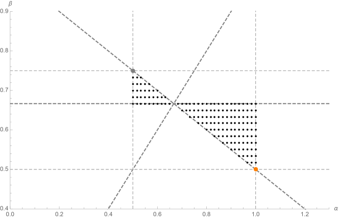
Figure 1: The figure shows the bowtie-shaped region ${\cal{B}}$ (see (27)) together with the grid ${\cal{G}}\subset{\cal{B}}$ in the parameter plane. The line $\beta=\alpha$ is also displayed (cf. (24)). The orange dot at $(\alpha,\beta)=(1,1/2)$ corresponds to the unique optimal ERK(3,3) method with ${\mathcal{C}}=1$. The gray dot at $(\alpha,\beta)=(1/2,3/4)$ corresponds to the unique ERK(3,3) method with minimum truncation-error coefficient.

In particular, Conjecture 1 means that there are infinitely many ERK(3,3) methods with step-size coefficient $\gamma=1$ in the present Case I (but see also Proposition 5, where we are going to actually prove that there are infinitely many ERK(3,3) methods with step-size coefficient $\gamma=1$ in Case II). In contrast, as stated earlier, there is only one ERK(3,3) method with SSP coefficient ${\mathcal{C}}=1$ (denoted by the orange dot in Figure 1).

It is a nice coincidence that the method with $(\alpha,\beta)=(1/2,3/4)$ (depicted as the gray vertex of ${\cal{B}}$ in Figure 1), that is, the one with tableau

$$A=\left(\begin{array}[]{ccc}0&0&0\\ \frac{1}{2}&0&0\\ 0&\frac{3}{4}&0\\ \end{array}\right),\quad b^{\top}=\left(\frac{2}{9},\frac{1}{3},\frac{4}{9}\right)$$ (28)

is also an element of ${\cal{B}}$: in the full ERK(3,3) family (i.e., in Cases I-III) this is the unique method having the minimum truncation-error coefficient [16, p. 433]. Therefore, for problems of type (10), the method (28) satisfies two optimality criteria simultaneously. The following proposition shows that this method indeed has the optimal step-size coefficient $\gamma=1$.

Proposition 3.

For each $i=0,1,2$ and all $(x,y,z,u,v,w)\in[0,1]^{6}$ we have

$$P_{i,1/2,3/4}(x,y,z,u,v,w)\geq 0.$$

Proof.

For any $(x,y,z,u,v,w)\in[0,1]^{6}$ we have

$$18P_{0,1/2,3/4}(x,y,z,u,v,w)=18-8w-4z+3v(1-w)(z-2)\geq 6+3v(1-w)(z-2)\geq 6-6=0,$$

$$18P_{1,1/2,3/4}(x,y,z,u,v,w)=3v(1-w)(2-y-z)+4z+w(8+3u(y-2))\geq w(8+3u(y-2))\geq 2w\geq 0,$$

and

$$6P_{2,1/2,3/4}(x,y,z,u,v,w)=uw(2-x-y)+yv(1-w)\geq 0.$$

∎

Remark 3.

The present approach does not fully explain results in [9] regarding 3rd-order methods. Therein, the method with $\alpha=1/3,\beta=2/3$ was found to give good results, but investigation of this method using the present technique yields that $\gamma=0$.

4.2 Case II

For any $\alpha\in\mathbb{R}\setminus\{0\}$, these ERK(3,3) methods are described by the tableau

$$A=\left(\begin{array}[]{ccc}0&0&0\\ \frac{2}{3}&0&0\\ \frac{2}{3}-\frac{1}{4\alpha}&\frac{1}{4\alpha}&0\\ \end{array}\right),\quad b^{\top}=\left(\frac{1}{4},\frac{3}{4}-\alpha,\alpha\right).$$ (29)

Regarding the SSP coefficient in this family, we have the following result (whose proof details are omitted here).

Proposition 4.

The SSP coefficient satisfies

$${\mathcal{C}}_{\alpha}=\begin{cases}0,&0\neq\alpha<\frac{3}{8}\\ \frac{8\alpha-3}{2},&\frac{3}{8}\leq\alpha\leq\frac{9}{16}\\ 3-4\alpha,&\frac{9}{16}<\alpha\leq\frac{3}{4}\\ 0,&\alpha>\frac{3}{4},\end{cases}$$ (30)

hence the unique maximum of the SSP coefficient occurs at ${\mathcal{C}}_{9/16}=3/4$.

Proposition 5.

The step-size coefficient in this family is given by

$$\gamma_{\alpha}=\begin{cases}0,&0\neq\alpha<\frac{3}{8}\\ 2\alpha,&\frac{3}{8}\leq\alpha<\frac{1}{2}\\ 1,&\frac{1}{2}\leq\alpha\leq\frac{3}{4}\\ 0,&\alpha>\frac{3}{4}.\end{cases}$$ (31)

Proof.

We use the polynomials and variables given by (22)-(23) now with (29).

For any fixed $0\neq\alpha<\frac{3}{8}$ and arbitrary $\varepsilon>0$ we have

$$12P_{2,\alpha}(0,\varepsilon,0,0,0,\varepsilon)=\varepsilon^{2}(8\alpha-3)<0,$$

showing that $\gamma_{\alpha}=0$ here.

For any fixed $\alpha>\frac{3}{4}$ and arbitrary $\varepsilon>0$ we have

$$6P_{2,\alpha}(\varepsilon,\varepsilon,\varepsilon,\varepsilon,\varepsilon,0)=\varepsilon^{2}(3-4\alpha)<0,$$

hence $\gamma_{\alpha}=0$ also holds for these values of $\alpha$.

For any fixed $\frac{3}{8}\leq\alpha<\frac{1}{2}$ and arbitrary $\varepsilon>0$ we have

$$3P_{2,\alpha}(2\alpha+\varepsilon,2\alpha+\varepsilon,2\alpha+\varepsilon,2\alpha+\varepsilon,0,2\alpha+\varepsilon)=-\varepsilon(2\alpha+\varepsilon)^{2}<0,$$

so $\gamma_{\alpha}\leq 2\alpha$ for these values of $\alpha$.

For any fixed $\frac{1}{2}\leq\alpha\leq\frac{3}{4}$ and arbitrary $\varepsilon>0$ we have

$$2P_{2,\alpha}(1+\varepsilon,1+\varepsilon,1+\varepsilon,1+\varepsilon,1+\varepsilon,1+\varepsilon)=-\varepsilon(1+\varepsilon)^{2}<0,$$

therefore $\gamma_{\alpha}\leq 1$ for these values of $\alpha$.

Since $P_{3}(x,y,z,u,v,w)=\frac{1}{6}xuw\geq 0$ for any non-negative choice of the arguments, to finish the proof of the proposition, we need to establish that

$$P_{0,\alpha}(x,y,z,u,v,w)\geq 0,\quad P_{1,\alpha}(x,y,z,u,v,w)\geq 0\quad\text{and}\quad P_{2,\alpha}(x,y,z,u,v,w)\geq 0$$

hold

• for any $\alpha\in\left[\frac{3}{8},\frac{1}{2}\right)$ and $(x,y,z,u,v,w)\in[0,2\alpha]^{6}$, implying $\gamma_{\alpha}\geq 2\alpha$;

• for any $\alpha\in\left[\frac{1}{2},\frac{3}{4}\right]$ and $(x,y,z,u,v,w)\in[0,1]^{6}$, implying $\gamma_{\alpha}\geq 1$.

Here we present the proof only for the case $\alpha\in\left[\frac{1}{2},\frac{3}{4}\right]$—yielding the maximum possible value of $\gamma_{\alpha}=1$ for infinitely many ERK(3,3) methods; the proof details in the other case (for $\alpha\in\left[\frac{3}{8},\frac{1}{2}\right)$) are analogous.

$\bullet$ Non-negativity of $P_{0,\alpha}$. We first show that $P_{0,\alpha}(x,y,z,u,v,w)\geq 0$ holds for any $\alpha\in\left[\frac{1}{2},\frac{3}{4}\right]$ and $(x,y,z,u,v,w)\in[0,1]^{6}$. Indeed,

$$12P_{0,\alpha}(x,y,z,u,v,w)=12\alpha v-2vwz+3vw-8\alpha vz+6vz-9v-12\alpha w+8\alpha wz-3wz-3z+12=$$

$$(12\alpha-9)v+vw(3-2z)+2(3-4\alpha)vz-12\alpha w+8\alpha wz-3(w+1)z+12\geq$$

$$\left(12\cdot\frac{1}{2}-9\right)\cdot 1+0+0-12\alpha w+8\alpha wz-3(1+1)z+12=-12\alpha w+8\alpha wz-6z+9=$$

$$(3-2z)(3-4\alpha w)\geq 0.$$

$\bullet$ Non-negativity of $P_{1,\alpha}$. Next we show that $P_{1,\alpha}(x,y,z,u,v,w)\geq 0$ holds for any $\alpha\in\left[\frac{1}{2},\frac{3}{4}\right]$ and $(x,y,z,u,v,w)\in[0,1]^{6}$. This time we have

$$12P_{1,\alpha}(x,y,z,u,v,w)=\big{[}-12\alpha v+8\alpha vy-6vy+8\alpha vz-6vz+9v+3z\big{]}+$$

$$w\big{[}12\alpha+2uy-3u+2vy+2vz-3v-8\alpha y+3y-8\alpha z+3z\big{]}.$$

We prove that both pairs of brackets $[\ldots]$ above contain non-negative quantities.

As for the first pair of brackets, notice that

$$-12\alpha v+8\alpha vy-6vy+8\alpha vz-6vz+9v+3z=-12\alpha v+8\alpha vy-6vy+8\alpha vz-3vz+3(1-v)z+9v\geq$$

$$-12\alpha v+8\alpha vy-6vy+8\alpha vz-3vz+0+9v=v(-12\alpha+(8\alpha-6)y+(8\alpha-3)z+9)\geq$$

$$v(-12\alpha+(8\alpha-6)y+0+9)=v(3-4\alpha)(3-2y)\geq 0.$$

As for the second pair of brackets, we have

$$12\alpha+2uy-3u+2vy+2vz-3v-8\alpha y+3y-8\alpha z+3z\geq$$

$$12\alpha+0\cdot uy-3\cdot 1+2vy+2vz-3v-8\alpha y+3y-8\alpha z+3z.$$

Now, by introducing $\rho:=2\alpha-1\in\left[0,\frac{1}{2}\right]$ and $\sigma:=y+z\in[0,2]=\left[0,\frac{3}{2}\right)\cup\left[\frac{3}{2},2\right]$, we get that the last expression above is equal to

$$3-\sigma+(2\sigma-3)(v-2\rho).$$

For $\sigma\in\left[0,\frac{3}{2}\right)$ we are done because

$$3-\sigma+(2\sigma-3)(v-2\rho)=3-\sigma+(2\rho-v)(3-2\sigma)\geq 3-\sigma+(0-1)(3-2\sigma)=\sigma\geq 0.$$

For $\sigma\in\left[\frac{3}{2},2\right]$ we are also done because

$$3-\sigma+(2\sigma-3)(v-2\rho)\geq 3-\sigma+(2\sigma-3)(v-1)\geq$$

$$1+(2\sigma-3)(v-1)\geq 1+(2\cdot 2-3)(v-1)=v\geq 0.$$

$\bullet$ Non-negativity of $P_{2,\alpha}$. Finally we show that $P_{2,\alpha}(x,y,z,u,v,w)\geq 0$ holds for any $\alpha\in\left[\frac{1}{2},\frac{3}{4}\right]$ and $(x,y,z,u,v,w)\in[0,1]^{6}$. We now have

$$12P_{2,\alpha}(x,y,z,u,v,w)=(3-2x)uw-2uwy-2vwy-8\alpha vy+6vy+8\alpha wy-3wy\geq$$

$$1\cdot uw-2uwy-2vwy-8\alpha vy+6vy+8\alpha wy-3wy=$$

$$uw(1-y)-uwy-2vwy-8\alpha vy+6vy+8\alpha wy-3wy\geq$$

$$0-uwy-2vwy-8\alpha vy+6vy+8\alpha wy-3wy=$$

$$y(-uw-2vw-8\alpha v+6v+8\alpha w-3w)\geq y(-1\cdot w-2vw-8\alpha v+6v+8\alpha w-3w)=$$

$$y(-8\alpha v-2vw+6v+8\alpha w-4w).$$

Clearly, to finish the proof, it is enough to show that

$$-8\alpha v-2vw+6v+8\alpha w-4w\geq 0.$$

By introducing $\rho:=2\alpha-1\in\left[0,\frac{1}{2}\right]$, the left-hand side of this last expression above becomes

$$-4(\rho+1)v-2vw+6v+4(\rho+1)w-4w.$$

If $w-v\geq 0$, then we are done, since

$$-4(\rho+1)v-2vw+6v+4(\rho+1)w-4w=4\rho(w-v)+2v(1-w)\geq 0.$$

If $w-v<0$, then we are also done, since

$$-4(\rho+1)v-2vw+6v+4(\rho+1)w-4w=4\rho(w-v)+2v(1-w)\geq$$

$$4\cdot\frac{1}{2}\cdot(w-v)+2v(1-w)=2(1-v)w\geq 0.$$

∎

Figure 2 displays the coefficients ${\mathcal{C}}_{\alpha}$ and $\gamma_{\alpha}$.

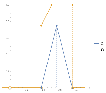
Figure 2: The SSP coefficient (30) and the step-size coefficient (31) in Case II

4.3 Case III

For any $\alpha\in\mathbb{R}\setminus\{0\}$, the ERK(3,3) methods within this family have the tableau

$$A=\left(\begin{array}[]{ccc}0&0&0\\ \frac{2}{3}&0&0\\ -\frac{1}{4\alpha}&\frac{1}{4\alpha}&0\\ \end{array}\right),\quad b^{\top}=\left(\frac{1}{4}-\alpha,\frac{3}{4},\alpha\right).$$ (32)

It can be proved that their SSP coefficient is trivial, that is,

$${\mathcal{C}}_{\alpha}=0\textrm{ for any }\alpha\neq 0.$$ (33)

As for the step-size coefficient, by using the polynomials and variables given in (22)-(23) with (32), we get for any $\varepsilon>0$ that

$$4P_{2,\alpha}(0,\varepsilon,0,0,0,\varepsilon)=-\varepsilon^{2}<0,$$

implying

$$\gamma_{\alpha}=0\textrm{ for any }\alpha\neq 0.$$ (34)

5 Step-size coefficients for higher-order methods

In this section we investigate the non-negativity of higher-order ERK methods and show some negative results.

It is known [6, Section 2.4.3] that the SSP coefficient for any ERK(4,4) method is ${\mathcal{C}}=0$. The question naturally arises whether it is possible to find an ERK(4,4) method with positive step-size coefficient.

First we recall the following result; see the proof of [15, Theorem 9.6], and of [6, Theorem 2.4].

Proposition 6.

A 4-stage 4th-order explicit Runge–Kutta method has non-negative Butcher tableau $(A,b)$ if and only if the method is the classical RK4 method (appearing in Appendix A.1).

Proposition 6 and Theorem 3 yield the following.

Proposition 7.

Any non-confluent ERK(4,4) method has step-size coefficient $\gamma=0$.

The previous result cannot be applied to the classical ERK(4,4) method, for example, which is confluent. For this method we have the following construction.

Proposition 8.

There is no positive step-size coefficient $\gamma$ such that the classical ERK(4,4) method preserves positivity for all problems of the form (10).

Proof.

We prove the proposition by constructing an ODE system (10) such that the method gives a negative solution value for any positive step size.

First we determine (for example, by using the code in Appendix A.1) that the polynomial $P_{3}$ for this method appearing in (14) is

$$P_{3}(x_{1},x_{2},x_{3},x_{4},x_{5},x_{6},x_{7},x_{8},x_{9},x_{10})=$$

$$\frac{1}{24}\left(2x_{2}x_{6}x_{9}+2x_{5}x_{8}x_{10}-x_{1}x_{5}x_{8}x_{10}-x_{2}x_{5}x_{8}x_{10}-x_{2}x_{6}x_{8}x_{10}-x_{2}x_{6}x_{9}x_{10}\right),$$

where, for better readability, we have relabeled the variables according to

$$(x_{1},x_{2},\ldots,x_{10}):=(\xi^{1}_{k-3},\xi^{1}_{k-2},\xi^{1}_{k-1},\xi^{1}_{k},\xi^{2}_{k-2},\xi^{2}_{k-1},\xi^{2}_{k},\xi^{3}_{k-1},\xi^{3}_{k},\xi^{4}_{k}).$$

We observe that this polynomial is negative in any hypercube $[0,\varepsilon]^{10}$ with $\varepsilon>0$, since

$$P_{3}(0,\varepsilon,0,0,0,\varepsilon,0,\varepsilon,0,\varepsilon)=-\varepsilon^{4}/24<0.$$

We now let $N=4$, $\varepsilon=\Delta t/\Delta x$, and as initial data take $v:=u(t_{0})=(1,0,0,0)$. Then $P_{3}(\xi)=-\varepsilon^{4}/24$ if $\xi_{k-2}^{1}=\xi_{k-1}^{2}=\xi_{k-1}^{3}=\xi_{k}^{4}=\varepsilon$ and the remaining values of $\xi$ are zero. Thus it remains only to choose a definition of the functions $q_{k}$ such that the aforementioned $\xi$ values result.

We can write the first step of the method as

$$y^{1} =v$$

$$y^{2}_{k} =v_{k}+\frac{\varepsilon}{2}q_{k}(y^{1})(y^{1}_{k-1}-y^{1}_{k})$$

$$y^{3}_{k} =v_{k}+\frac{\varepsilon}{2}q_{k}(y^{2})(y^{2}_{k-1}-y^{2}_{k})$$

$$y^{4}_{k} =v_{k}+\varepsilon q_{k}(y^{3})(y^{3}_{k-1}-y^{3}_{k})$$

$$u^{1}_{k} =v_{k}+\frac{\varepsilon}{6}\left(q_{k}(y^{1})(y^{1}_{k-1}-y^{1}_{k})+2q_{k}(y^{2})(y^{2}_{k-1}-y^{2}_{k})+2q_{k}(y^{3})(y^{3}_{k-1}-y^{3}_{k})+q_{k}(y^{4})(y^{4}_{k-1}-y^{4}_{k})\right).$$

We have $y^{1}=u(t_{0})=(1,0,0,0)$, and we define $q_{2}(y^{1})=1$, while $q_{1}(y^{1})=q_{3}(y^{1})=q_{4}(y^{1})=0$. This leads to $y^{2}=(1,\varepsilon/2,0,0)$, and we define $q_{3}(y^{2})=1$, while $q_{1}(y^{2})=q_{2}(y^{2})=q_{4}(y^{2})=0$. This leads to $y^{3}=(1,0,\varepsilon^{2}/4,0)$, and we define $q_{3}(y^{3})=1$, while $q_{1}(y^{3})=q_{2}(y^{3})=q_{4}(y^{3})=0$. This leads to $y^{4}=(1,0,-\varepsilon^{3}/4,0)$, and we define $q_{4}(y^{4})=1$, while $q_{1}(y^{4})=q_{2}(y^{4})=q_{3}(y^{4})=0$. This leads to $u^{1}=(1,\varepsilon/6,(2\varepsilon^{2}-\varepsilon^{3})/12,-\varepsilon^{4}/24)$. The last entry is negative for any positive step size, and the proof is complete. ∎

Some well-known ERK methods of higher order or with more stages—e.g., the methods of Fehlberg [5] or Dormand-Prince [4]—contain negative entries in their Butcher tableau, so Theorem 3 shows that their step-size coefficient is 0. Nevertheless, we have constructed some ERK(5,7) methods with non-negative tableau (see [18] also). For these methods however the approach described in Section 2.2 becomes practically unmanageable with our current tools: one would need to test the non-negativity of multivariable polynomials with several hundred terms in high-dimensional hypercubes.

6 Discussion and further applications

The method described and applied herein can be employed to study positivity and related properties for any semi-discretization that can be written in the form

$$u^{\prime}_{k}(t) =q_{k}(u(t),t)\sum_{j=-r}^{r}c_{j}u_{k-j}(t),$$

where $q_{k}\geq 0$. Given this form, we can determine polynomials such that

$$u_{k}^{n+1} =\sum_{i=-rm}^{rm}P_{i}(\xi)u_{k-i}^{n},$$ (35)

following the approach in Section 2.1; only the structure of the matrix $D$ changes in (15).

The computationally expensive step in the analysis is the determination of a hypercube—in the non-negative orthant, and preferably having the maximum edge length—in which the polynomials $P_{i}$ (depending on parameters if we are to optimize in parametric families of ERK methods) are simultaneously non-negative. The limiting factor is the dimension of the hypercubes, as it grows quadratically with the number of stages of the method. With current tools, methods with more than five stages cannot easily be studied in this manner. Nevertheless, the necessary condition for non-negativity obtained by evaluating the polynomials $P_{i}$ at the hypercube vertices often turns out to be sufficient as well (sufficiency can be proved by examining the critical points and the boundaries). Moreover, Theorem 3 immediately provides negative conclusions regarding many high-order methods.

It is worthwhile to return to a comparison of this approach with that of strong stability preserving methods. The essential differences are the following.

• In the current approach, we consider a more restricted class of problems; however, this class contains the principal class of problems for which SSP theory was developed.

• In the current approach, it is not necessary that the forward Euler method be positive in order to prove positivity for higher-order methods. Nevertheless, in all cases studied so far, we have obtained positive step sizes only for semi-discretizations that are stable under forward Euler integration.

• The current approach gives larger step sizes than the SSP approach for many methods.

Both approaches are still overly pessimistic for certain methods of interest, such as the classical 4-stage 4th-order method, which cannot be guaranteed positive with either approach but yields good results in practice. It may be possible to obtain sharper step-size restrictions for such methods by either restricting the allowed initial data or invoking some assumption of consistency on values of $q$ generated from one stage to the next (both approaches would lead to consideration of positivity of the polynomials $P_{i}$ on sets other than hypercubes).

In the remainder of this section, we demonstrate the application of these techniques to some additional semi-discretizations.

6.1 Centered discretizations of hyperbolic problems

Let us consider centered semi-discretizations of the form

$$u^{\prime}(t)=Q(u(t),t)Du(t),$$ (36)

where $Q$ is diagonal and $D$ is skew-symmetric. Such discretizations arise when centered finite differences are applied to a hyperbolic problem. For example,

$$u^{\prime}_{k}(t) =q_{k}(u(t),t)\frac{u_{k-1}(t)-u_{k+1}(t)}{2\Delta x},\quad k=1,\ldots,N$$ (37)

with $q=1$ is a common semi-discretization of the advection equation $U_{t}+U_{x}=0$. Since the exact solution of this system of ODEs does not preserve positivity, any consistent semi-discretization will also not be positivity-preserving for sufficiently small step sizes. Below, we show how this conclusion can be reached directly using the present technique.

For such discretizations, we have the following result, which follows from the fact that odd powers of $D$ are skew-symmetric while even powers are symmetric.

Lemma 1.

Let a semi-discretization (36) be given with $Q$ diagonal and $D$ skew symmetric. Define the vector $\hat{\xi}$ such that $\hat{\xi}_{k+i}^{j}:=\xi_{k-i}^{j}$. For any Runge–Kutta method applied to this semi-discretization, we have an iteration of the form (35), where

$$P_{j}(\xi) =P_{-j}(\hat{\xi}) j$$ for even;

$$P_{j}(\xi) =-P_{-j}(\hat{\xi}) j$$ for odd.

The latter equality for the odd-numbered polynomials generally implies that no positive step-size coefficient exists.

6.2 The heat equation

As a next example, we consider the scalar heat equation $U_{t}=\kappa(x)U_{xx}$ and its semi-discretization in the form

$$u^{\prime}_{k}(t)=\displaystyle q_{k}\ \frac{u_{k-1}(t)-2u_{k}(t)+u_{k+1}(t)}{(\Delta x)^{2}},\quad k=1,\ldots,N,$$ (38)

where $u_{0}:=u_{N},\ u_{N+1}:=u_{1}$, and $q_{k}=\kappa(x_{k})\geq 0$. The matrix $D_{N}$ in (16) is now the $N\times N$ tridiagonal matrix with entries $(1,-2,1)$ such that $[D_{N}]_{1,N}=[D_{N}]_{N,1}=1$.

When, for example, a two-stage ERK method is applied to (38), the $k^{\textrm{th}}$ component of the step solution in (16) becomes

$$u^{n+1}_{k}=P_{-2}(\xi)u^{n}_{k+2}+P_{-1}(\xi)u^{n}_{k+1}+P_{0}(\xi)u^{n}_{k}+P_{1}(\xi)u^{n}_{k-1}+P_{2}(\xi)u^{n}_{k-2},$$

where

$$P_{-2}(\xi)=\ a_{21}b_{2}\xi_{k+1}^{1}\xi_{k}^{2},$$

$$P_{-1}(\xi)=\ b_{1}\xi_{k}^{1}+b_{2}\xi_{k}^{2}-2a_{21}b_{2}\xi_{k}^{1}\xi_{k}^{2}-2a_{21}b_{2}\xi_{k+1}^{1}\xi_{k}^{2},$$

$$P_{0}(\xi)=\ 1-2b_{1}\xi_{k}^{1}-2b_{2}\xi_{k}^{2}+a_{21}b_{2}\xi_{k-1}^{1}\xi_{k}^{2}+4a_{21}b_{2}\xi_{k}^{1}\xi_{k}^{2}+a_{21}b_{2}\xi_{k+1}^{1}\xi_{k}^{2},$$

$$P_{1}(\xi)=\ b_{1}\xi_{k}^{1}+b_{2}\xi_{k}^{2}-2a_{21}b_{2}\xi_{k-1}^{1}\xi_{k}^{2}-2a_{21}b_{2}\xi_{k}^{1}\xi_{k}^{2},$$

$$P_{2}(\xi)=\ a_{21}b_{2}\xi_{k-1}^{1}\xi_{k}^{2}$$

and

$$\xi_{k}^{j}=\frac{\Delta t}{(\Delta x)^{2}}q_{k},\quad j=1,\ldots,m.$$

By introducing the variables

$$x:=\xi_{k-1}^{1},\ y:=\xi_{k}^{1},\ z:=\xi_{k+1}^{1},\ u:=\xi_{k}^{2}$$

and using (18), the multivariable polynomials corresponding to the ERK(2,2) family are now

$$P_{-2}(x,y,z,u)=\ \frac{uz}{2},$$

$$P_{-1}(x,y,z,u)=\ \frac{u-y-2\alpha(yu+uz-y)}{2\alpha},$$

$$P_{0}(x,y,z,u)=\ \frac{u(\alpha x+4\alpha y+\alpha z-2)+2(\alpha-2\alpha y+y)}{2\alpha},$$

$$P_{1}(x,y,z,u)=\ \frac{u-y-2\alpha(xu+yu-y)}{2\alpha},$$

$$P_{2}(x,y,z,u)=\ \frac{xu}{2}.$$

This time, unlike in Section 6.1, we get non-trivial step-size coefficients in the ERK(2,2) family.

Proposition 9.

We have

$$\gamma_{\alpha}\begin{cases}=1/2,&\alpha\in[1/2,1]\\ <1/2,&0\neq\alpha<1/2\textrm{ or }\alpha>1.\end{cases}$$

Proof.

For any fixed $\alpha\neq 0$, we are looking for some $\varepsilon\equiv\varepsilon(\alpha)>0$ such that the inequalities $P_{i}\geq 0$ for $-2\leq i\leq 2$ hold in $[0,\varepsilon]^{4}$. Clearly, it is enough to consider the indices $i=-1,0,1$. By again investigating the vertices of the hypercube $[0,\varepsilon]^{4}$ (see Appendix A.2), we derive the necessary conditions

$$\left(\frac{1}{2}\leq\alpha\leq 1\text{ and }0<\varepsilon\leq\frac{1}{2}\right)\text{ or }\left(\alpha>1\text{ and }0<\varepsilon\leq\frac{1}{2\alpha}\right).$$

By considering the maximum value $\varepsilon=1/2$, we can then prove that for any $\alpha\in[1/2,1]$ and any $(x,y,z,u)\in[0,1/2]^{4}$ we indeed have $P_{-1}\geq 0$, $P_{0}\geq 0$ and $P_{1}\geq 0$. ∎

Appendix A Some Mathematica code

A.1 Generating the multivariable polynomials

The first cell below contains the definition of a Mathematica function ERKpolynomials for generating the multivariable polynomials in (14). The two arguments $A$ and $b$ correspond to the Butcher tableau of the ERK method, and the output is a list of the $m+1$ polynomials $P_{0}$, …, $P_{m}$ in the variables $\xi_{\ell}^{j}$. Note that the superscripts in $\xi_{\ell}^{j}$ are not exponents; the symbols $\xi_{\ell}^{j}$ with different sub- or superscripts denote different variables.

The second cell illustrates how to obtain the $4+1=5$ polynomials in $\frac{4\cdot(4+1)}{2}=10$ variables corresponding to the classical ERK(4,4) method.

 

ERKpolynomials[A_,b_]:= Module[{m=Length@b,xi,S},ClearAll[\[Xi],k];
   xi=DiagonalMatrix@Table[Subsuperscript[\[Xi],k,i],{i,m}];
   CoefficientList[1+First[
   b.xi.Total@NestList[A.(DiscreteShift[S xi.#,{k,-1}]-xi.#)&,IdentityMatrix[m],m-1].
   ConstantArray[S-1,{m,1}]],S]]

 

ERKpolynomials[{{0,0,0,0},{1/2,0,0,0},{0,1/2,0,0},{0,0,1,0}},{1/6,1/3,1/3,1/6}]

 

A.2 Non-negativity of polynomials at the vertices of a hypercube

Here we provide a simple Mathematica code to test the non-negativity of a multivariable polynomial by evaluating it at each vertex of a hypercube. In this particular example, the polynomial $P_{-1}(x,y,z,u)$ from Section 6.2 is evaluated at the $2^{4}$ vertices of the hypercube $[0,\varepsilon]^{4}$ with some $\varepsilon>0$, and the resulting system of 16 inequalities $P_{-1}\geq 0$ is solved.

   $\texttt{Reduce\Big{[}}\varepsilon>0\texttt{\,\&\&\,And\,@@}\Big{(}{\displaystyle 0\leq\frac{u-y-2\alpha(y\ u+u\ z-y)}{2\alpha}}\texttt{/.}$

  $\texttt{Thread\,/@\,Table\big{[}}{\displaystyle\{x,y,z,u\}\to}\texttt{\,Tuples[}\{0,\varepsilon\}\texttt{,4][[k]],}\{\texttt{k},1,2^{4}\}\texttt{\big{]}}\Big{)}\texttt{\Big{]}}$
 

Acknowledgement. We are indebted to the referees of the manuscript for their suggestions that helped us improving the presentation of the material.

References

- [1] C. Bolley and M. Crouzeix. Conservation de la positivité lors de la discrétisation des problémes d’évolution paraboliques. R.A.I.R.O. Analyse Numérique, 12(3):237–245, 1978.
- [2] J. C. Butcher. Numerical methods for ordinary differential equations. John Wiley & Sons, Ltd., Chichester, second edition, 2008.
- [3] G. Dahlquist and R. Jeltsch. Reducibility and contractivity of Runge–Kutta methods revisited. Bit Numerical Mathematics, 46:567–587, 2006.
- [4] J. R. Dormand and P. J. Prince. A family of embedded Runge–Kutta formulae. Journal of Computational and Applied Mathematics, 6(1):19–26, 1980.
- [5] E. Fehlberg. Klassische Runge–Kutta-Formeln fünfter und siebenter Ordnung mit Schrittweiten-Kontrolle. Computing, 4(2):93–106, 1969.
- [6] S. Gottlieb, D. Ketcheson, and C.-W. Shu. Strong stability preserving Runge–Kutta and multistep time discretizations. World Scientific Publishing Co. Pte. Ltd., Hackensack, NJ, 2011.
- [7] A. Harten. High resolution schemes for hyperbolic conservation laws. Journal of Computational Physics, 49:357–393, 1983.
- [8] I. Higueras. Strong stability for Runge–Kutta schemes on a class of nonlinear problems. J. Sci. Comput., 57(3):518–535, 2013.
- [9] W. Hundsdorfer, B. Koren, M. van Loon, and J. G. Verwer. A positive finite-difference advection scheme. Journal of Computational Physics, 117(1):35–46, 1995.
- [10] W. Hundsdorfer and J. Verwer. Numerical solution of time-dependent advection-diffusion-reaction equations, volume 33 of Springer Series in Computational Mathematics. Springer-Verlag, Berlin, 2003.
- [11] D. I. Ketcheson and A. C. Robinson. On the practical importance of the SSP property for Runge–Kutta time integrators for some common Godunov-type schemes. International Journal for Numerical Methods in Fluids, 48(3):271–303, May 2005.
- [12] M. M. Khalsaraei. An improvement on the positivity results for 2-stage explicit Runge–Kutta methods. J. Comput. Appl. Math., 235(1):137–143, 2010.
- [13] M. M. Khalsaraei. Positivity of an explicit Runge–Kutta method. Ain Shams Engineering Journal, 6(4):1217–1223, 2015.
- [14] B. Koren. A robust upwind discretization method for advection, diffusion and source terms. In Numerical methods for advection-diffusion problems, volume 45 of Notes Numer. Fluid Mech., pages 117–138. Vieweg, Braunschweig, 1993.
- [15] J. F. B. M. Kraaijevanger. Contractivity of Runge–Kutta methods. BIT, 31(3):482–528, 1991.
- [16] A. Ralston. Runge–Kutta methods with minimum error bounds. Math. Comp., 16:431–437, 1962.
- [17] P. L. Roe. Characteristic-based schemes for the Euler equations. In Annual review of fluid mechanics, Vol. 18, pages 337–365. Annual Reviews, Palo Alto, CA, 1986.
- [18] S. J. Ruuth and R. J. Spiteri. Two barriers on strong-stability-preserving time discretization methods. In Proceedings of the Fifth International Conference on Spectral and High Order Methods (ICOSAHOM-01) (Uppsala), volume 17, pages 211–220, 2002.
- [19] B. van Leer. Towards the ultimate conservative difference scheme. III - Upstream-centered finite-difference schemes for ideal compressible flow. IV - A new approach to numerical convection. Journal of Computational Physics, 23:263–299, March 1977.