Optomechanical dual-beam backaction-evading measurement
beyond the rotating-wave approximation

Abstract

We present the exact analytical solution of the explicitly time-periodic quantum Langevin equation describing the dual-beam backaction-evasion measurement of a single mechanical oscillator quadrature due to Braginsky, Vorontsov and Thorne beyond the commonly used rotating-wave approximation. We show that counterrotating terms lead to extra sidebands in the optical and mechanical spectra and to a modification of the main peak. Physically, the backaction of the measurement is due to periodic coupling of the mechanical resonator to a light field quadrature that only contains cavity-filtered shot noise. Since this fact is independent of other degrees of freedom the resonator might be coupled to, our solution can be generalized, including to dissipatively or parametrically squeezed oscillators, as well as recent two-mode backaction evasion measurements.

I Introduction

A continuous measurement of the position of a harmonic oscillator is subject to the “standard quantum limit” (SQL), a limit directly imposed by Heisenberg’s uncertainty relation Caves et al. (1980); Clerk et al. (2010). An observable that can be monitored without precision limit is called “quantum non-demolition” (QND) variable, such that its continuous measurement can avoid the measurement backaction (BA) Braginsky et al. (1980) and thus open the way to the detection of weak forces, such as those due to gravitational waves Abbott and Others (2016).

There has been continued interest to implement backaction-evading (BAE) measurements Bocko and Onofrio (1996). Following a detailed theoretical proposal, the first demonstration with a sensitivity beyond the SQL was in optomechanics Clerk et al. (2008); Hertzberg et al. (2010) and they have since proven very useful Suh et al. (2014); Lecocq et al. (2015); Lei et al. (2016); Polzik and Hammerer (2014). Despite the importance of such measurements, Ref. Clerk et al. (2008) discusses only lowest-order corrections to the rotating-wave approximation (RWA).

Here, using the recently developed Floquet approach Malz and Nunnenkamp (2016), we derive the exact solution to the equations describing a BAE measurement. Due to the presence of CR terms, this constitutes a solution to genuinely explicitly time-dependent quantum Langevin equations, as there is no frame in which they become stationary. The solution is possible because the mechanical oscillator couples solely to a light quadrature that is independent of the mechanical oscillator, and only contains filtered shot noise. The coupling is periodic, which leads to two-time correlators that are not time-translation invariant. In such a situation, the power spectrum is a time average of the Fourier transform of the autocorrelator Malz and Nunnenkamp (2016).

In the following, after introducing our model in Section II, we briefly remind the reader of results in RWA in Section III. Then, we present all aspects of the solution, from the Floquet framework to the resulting spectra and backaction in Section IV. Finally, in Section V, we show how to generalize our solution to the important cases of dissipative and parametric squeezing, as well as two-mode BAE measurements (with explicit calculations in Appendices D, A, B and C). We conclude in Section VI.

II Model

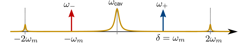
Figure 1: The dual-beam backaction-evading (BAE) measurement scheme proposed in Ref. Braginsky et al. (1980); Clerk et al. (2008). Two lasers of equal strength drive the cavity at frequencies $\omega_{\pm}=\omega_{\text{cav}}\pm\delta$, where $\delta=\omega_{m}$ such that their sidebands overlap at the cavity frequency $\omega_{\text{cav}}$. Counterrotating (CR) terms cause peaks at $\omega_{\text{cav}}\pm 2\omega_{m}$ to appear. The output light will be an approximate BAE measurement of a rotating quadrature of the mechanical oscillator, the CR terms being responsible for the finite backaction.

In cavity optomechanics, the photons in a cavity couple to the motion of a mirror via radiation pressure. A BAE measurement of one of the quadratures of the oscillator can be implemented by applying two drives of equal strength at frequencies $\omega_{\text{cav}}\pm\omega_{m}$ (see Fig. 1). Here, $\omega_{\text{cav}}(\omega_{m})$ is the frequency of a cavity (mechanical) mode. Originally due to Braginsky et al. Braginsky et al. (1980), the first detailed analysis in the context of cavity optomechanics was given in Ref. Clerk et al. (2008).

We consider the Hamiltonian of a standard cavity optomechanical system

$$H=H_{\text{OM}}+H_{\text{rest}}+H_{\text{drives}}+H_{\text{baths}},$$ (1)

where ($\hbar=1$)

$$H_{\text{OM}} =\omega_{\text{cav}}a^{\dagger}a+\omega_{m}b^{\dagger}b-g_{0}a^{\dagger}a(b^{\dagger}+b),$$ (2a)

$$H_{\text{drives}} =\alpha(e^{-i\omega_{+}t}+e^{-i\omega_{-}t})a^{\dagger}+\text{h.c.}$$ (2b)

$a,b$ are the bosonic annihilation operators of the cavity mode and the mechanical oscillator, respectively. The cavity mode frequency is $\omega_{\text{cav}}$, the mechanical frequency $\omega_{m}$, the coupling strength via radiation pressure $g_{0}$, and the driving strength of the drives with frequencies $\omega_{\pm}=\omega_{\text{cav}}\pm\delta$ is $\alpha$, where we have left $\delta$ unspecified for now (Fig. 1). The BAE measurement is realized for $\delta=\omega_{m}$. A detailed derivation of the optomechanical Hamiltonian can be found for instance in Ref. Aspelmeyer et al. (2014). $H_{\text{baths}}$ couples the oscillator and cavity modes to baths at finite and zero temperature, respectively. $H_{\text{rest}}$ will remain unspecified for now, it can contain terms that couple the harmonic oscillator to other degrees of freedom. The only requirement is that $[H_{\text{rest}},a+a^{\dagger}]=0$, i.e., that the other degrees of freedom do not couple to this measurement cavity quadrature.

To proceed, we split the light field into a coherent part and fluctuations, go into a rotating frame, $a=\bar{a}e^{-i\omega_{\text{cav}}t}(e^{i\delta t}+e^{-i\delta t}+d)$, and linearize the Hamiltonian. Without loss of generality, $\delta>0$. Under the usual assumptions of Markovian baths and a one-sided cavity, the resulting Hamiltonian

$$H=\omega_{m}b^{\dagger}b-2G\cos(\delta t)(b+b^{\dagger})(d+d^{\dagger})$$ (3)

gives rise to Langevin equations Gardiner and Zoller (2004); Clerk et al. (2010) that are periodic in time

$$\dot{d} =-\frac{\kappa}{2}d+\sqrt{\kappa}d_{\text{in}}+2iG\cos(\delta t)(b+b^{\dagger}),$$ (4a)

$$\dot{b} =\left(-i\omega_{m}-\frac{\gamma}{2}\right)b+\sqrt{\gamma}b_{\text{in}}$$

$$\qquad+2iG\cos(\delta t)(d+d^{\dagger})+i[H_{\text{rest}},b].$$ (4b)

Here, we have defined the enhanced optomechanical coupling constant $G=g_{0}\bar{a}$, and the mechanical (optical) dissipation rate $\gamma$ ($\kappa$). $b_{\text{in}},d_{\text{in}}$ are input noise operators with $\langle d_{\text{in}}(t)d_{\text{in}}^{\dagger}(t^{\prime})\rangle=\delta(t-t^{\prime})$, $\langle d_{\text{in}}^{\dagger}(t)d_{\text{in}}(t^{\prime})\rangle=0$, $\langle b_{\text{in}}(t)b_{\text{in}}^{\dagger}(t^{\prime})\rangle=(n_{\text{th}}+1)\delta(t-t^{\prime})$, and $\langle b_{\text{in}}^{\dagger}(t)b_{\text{in}}(t^{\prime})\rangle=n_{\text{th}}\delta(t-t^{\prime})$.

In Section IV.1, we solve Eqs. 4a and 4b without further approximations, in particular without the rotating wave approximation (RWA).

III Backaction evasion in RWA

As a reminder, we first consider a BAE measurement within RWA. We define a quadrature rotating a frequency $\delta$ as

$$X_{\delta}=be^{i\delta t}+b^{\dagger}e^{-i\delta t}.$$ (5)

The cavity equation of motion is (cf. Eq. 4a)

$$\dot{d}=-\frac{\kappa}{2}d+\sqrt{\kappa}d_{\text{in}}+iG\left(be^{i\delta t}+b^{\dagger}e^{-i\delta t}\right).$$ (6)

The cavity couples only to one quadrature of the mechanical oscillator $X_{\delta}$ (set by the phase relation of the external drives). The equation of motion for that quadrature can be obtained from Eq. 4b (here also in RWA)

$$\dot{X_{\delta}}=-\frac{\gamma}{2}X_{\delta}+\sqrt{\gamma}X_{\delta,\text{in}}+i[H_{\text{rest}},X_{\delta}]\\ +iG\left[d\left(e^{i(\omega_{m}-\delta)t}-e^{i(\delta-\omega_{m})t}\right)-\text{h.c.}\right].$$ (7)

If $\delta=\omega_{m}$, the term in square brackets in the second line vanishes, and $X_{\omega_{m}}$ is entirely unaffected by the cavity. We can readily solve the equation of motion for $d$, Eq. 6

$$d(\omega)=\chi_{c}(\omega)\left[\sqrt{\kappa}d_{\text{in}}(\omega)+iGX_{\delta}(\omega)\right],$$ (8)

with cavity response function $\chi_{c}(\omega)=(\kappa/2-i\omega)^{-1}$. Thus the optical spectrum is directly related to the quadrature spectrum

$$S_{d^{\dagger}d}(\omega)=|\chi_{c}(\omega)|^{2}G^{2}S_{X_{\delta}X_{\delta}}(\omega),$$ (9)

where for a stationary process the Wiener-Khinchin theorem ensures that the Fourier transform

$$S_{AB}(\omega)=\int_{-\infty}^{\infty}\differential{t}e^{i\omega t}\expectationvalue{A(t)B(0)}$$ (10)

is the quantum noise spectral density. The scheme corresponds to a true BAE measurement, if the mechanical quadrature rotating with frequency $\delta$ is a QND variable. Here, this is the case for $\delta=\omega_{m}$ (or, if applicable, $\delta=\omega_{m,\text{eff}}$, the effective mechanical frequency). Independent of RWA, the input-output relation $d_{\text{out}}=d_{\text{in}}-\sqrt{\kappa}d$ can be used to the obtain the output spectrum $S_{d_{\text{out}}^{\dagger}d_{\text{out}}}(\omega)=\kappa S_{d^{\dagger}d}(\omega).$ For details on how to measure and interpret the output spectrum, see Ref. Weinstein et al. (2014).

IV Floquet framework

The analysis in Section III above breaks down if we include counterrotating (CR) terms. Using the framework developed in Ref. Malz and Nunnenkamp (2016), it is possible to find the stationary state of the explicitly time-periodic quantum Langevin equations exactly, which gives us the opportunity to precisely determine the backaction of the BAE measurement.

First, we split system operators into Fourier components

$$d(t) =\sum_{n=-\infty}^{\infty}e^{in\delta t}d^{(n)}(t),$$ (11a)

$$d^{\dagger}(t) =\sum_{n=-\infty}^{\infty}e^{in\delta t}d^{(n){\dagger}}(t),$$ (11b)

and define

$$d^{(n)}(\omega) =\int_{-\infty}^{\infty}\differential{t}e^{i\omega t}d^{(n)}(t),$$ (12a)

$$d^{(n){\dagger}}(\omega) =\int_{-\infty}^{\infty}\differential{t}e^{i\omega t}d^{(n){\dagger}}(t).$$ (12b)

Note that this convention results in $[d^{(n)}(\omega)]^{\dagger}=d^{(-n){\dagger}}(-\omega)$. The reason for doing this is that Eqs. 4a and 4b can now be written as an infinite set of coupled, stationary Langevin equations

$$\dot{d}^{(n)}=\left(-in\delta-\frac{\kappa}{2}\right)d^{(n)}+\delta_{n,0}\sqrt{\kappa}d_{\text{in}}\\ +iG\left(b^{(n-1)}+b^{(n+1){\dagger}}+\lambda b^{(n+1)}+\lambda b^{(n-1){\dagger}}\right),$$ (13a)

$$\dot{b}^{(n)}=\left(-i\omega_{m}-in\delta-\frac{\gamma}{2}\right)b^{(n)}+\delta_{n,0}\sqrt{\gamma}b_{\text{in}}\\ +iG\left(I^{(n+1)}+\lambda I^{(n-1)}\right)+i[H_{\text{rest}},b]^{(n)}.$$ (13b)

where $x^{(n)}\equiv b^{(n)}+b^{(n){\dagger}}$, $I^{(n)}\equiv d^{(n)}+d^{(n){\dagger}}$, $\delta_{n,0}$ is the Kronecker delta, and $[H_{\text{rest}},b]^{(n)}$ is the $n$th Fourier component of the commutator. Where feasible, here and in the following, we will mark counterrotating (i.e., off-resonance) terms by a $\lambda$ (note that this only makes sense when $\delta$ is close to $\omega_{m}$), such that RWA corresponds to $\lambda=0$ and the full solution to $\lambda=1$. To further guide the intuition, we remark that the second line of Eq. 13a equals $iG(x^{(n-1)}+x^{(n+1)})$. One can think of the two laser drives to result in two separate couplings to the position $x$ of the resonator.

We define the “spectrum”

$$S_{A^{\dagger}A}(\omega,t)\equiv\int_{-\infty}^{\infty}\differential{\tau}e^{i\omega\tau}C_{AA}(\tau,t),$$ (14)

with $C_{AA}(\tau,t)\equiv\expectationvalue{A^{\dagger}(t+\tau)A(t)}$. The time dependence of $S_{A^{\dagger}A}(\omega,t)$ can be expressed as a Fourier series Malz and Nunnenkamp (2016)

$$S_{A^{\dagger}A}(\omega,t)=\sum_{n=-\infty}^{\infty}e^{i\delta nt}S_{A^{\dagger}A}^{(n)}(\omega)$$ (15)

with components

$$S_{A^{\dagger}A}^{(m)}(\omega)=\sum_{n}\int\frac{\differential{\omega^{\prime}}}{2\pi}\expectationvalue{A^{(n){\dagger}}(\omega+n\delta)A^{(m-n)}(\omega^{\prime})}.$$ (16)

It can be shown that the zeroth Fourier component, which at the same time is the time average of $S(\omega,t)$, is the measured power spectrum Malz and Nunnenkamp (2016).

IV.1 Solution beyond RWA

To solve Eqs. 4a and 4b, we define the optical quadratures $I=d+d^{\dagger}$ and $Q=-i(d-d^{\dagger})$. From Eq. 4a we obtain

$$\dot{I} =-\frac{\kappa}{2}I+\sqrt{\kappa}I_{\text{in}},$$ (17a)

$$\dot{Q} =-\frac{\kappa}{2}Q+\sqrt{\kappa}Q_{\text{in}}+4G\cos(\delta t)x.$$ (17b)

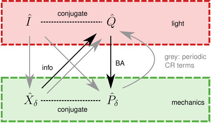
Figure 2: Coupling of quadratures. $\hat{Q}$ records the desired information (info) about $\hat{X}_{\delta}$. The measurement backaction (BA) is acting on $\hat{P}_{\delta}$. Marked in gray are coupling due to counterrotating (CR) terms that are neglected in RWA.

For an illustration how the mechanical and optical quadratures couple together, see Fig. 2. For example, the arrow from $X_{\delta}$ to $Q$ indicates that $X_{\delta}$ appears in the equation of motion of $Q$ and that the latter therefore is influenced by the former. Since $I$ commutes with the system Hamiltonian (3), $[H,I]=0$, there are no arrows pointing toward it in Fig. 2 and we can solve its equation of motion (17a) directly

$$I(\omega)=\sqrt{\kappa}\chi_{c}(\omega)I_{\text{in}}(\omega),\quad\text{and}\quad I^{(n)}(\omega)=\delta_{n,0}I(\omega).$$ (18)

Thus $\expectationvalue{I(\omega)I(\omega^{\prime})}=2\pi\delta(\omega+\omega^{\prime})|\chi_{c}(\omega)|^{2}$ and $\expectationvalue{I(\omega)}=0$. Equations 17a and 18 imply that $I$ is shot noise, filtered by the cavity, and is independent of the mechanics. Furthermore, this result does not depend on $H_{\text{rest}}$, as long as $[H_{\text{rest}},I]=0$. The coupling to $I$ is periodic (cf. Eq. 4b), a consequence of amplitude beating of the coherent state in the cavity. Therefore, the measurement has the same effect on the mechanical resonator as a time-periodic coupling to filtered shot noise.

With Eq. 18 we can solve Eq. 13b in the case $H_{\text{rest}}=0$ by going into frequency space

$$b^{(n)}(\omega) =\chi_{m}(\omega-n\delta)\left[\delta_{n,0}\sqrt{\gamma}b_{\text{in}}+2\sqrt{\kappa}Gf_{\text{in}}^{(n)}\right],$$ (19a)

$$b^{(n){\dagger}}(\omega) =\chi_{m}^{*}(-\omega+n\delta)\left[\delta_{n,0}\sqrt{\gamma}b_{\text{in}}^{\dagger}-2\sqrt{\kappa}Gf_{\text{in}}^{(n)}\right],$$ (19b)

where the new bath noise operators

$$f_{\text{in}}^{(n)}(\omega)=i\chi_{c}(\omega)(\delta_{n,1}+\lambda\delta_{n,-1})I_{\text{in}}(\omega)/2.$$ (20)

They obey $f_{\text{in}}^{(n){\dagger}}=-f_{\text{in}}^{(n)}$, $f_{\text{in}}^{(-n)}=f_{\text{in}}^{(n)}$, and $\expectationvalue{f_{\text{in}}}=0$. The time-dependence is best seen in the time domain, where

$$f_{\text{in}}(t)=i\cos(\delta t)I(t)/\sqrt{\kappa}.$$ (21)

This expression explicitly contains the time-dependent coupling and the filtered shot noise $I(t)$. The correlator is

$$\expectationvalue{f_{\text{in}}(t)f_{\text{in}}(t^{\prime})}=-e^{-\kappa|t-t^{\prime}|/2}\cos(\delta t)\cos(\delta t^{\prime}).$$ (22)

For stationary noise, the RHS of Eq. 22 would have to depend solely on the difference $t-t^{\prime}$.

We can rewrite the equation of motion for $b$ in terms of the new input $f_{\text{in}}$

$$\dot{b}=\left(-i\omega_{m}-\frac{\gamma}{2}\right)b+\sqrt{\gamma}b_{\text{in}}+2\sqrt{\kappa}Gf_{\text{in}}+i[H_{\text{rest}},b].$$ (23)

From this equation it is clear that we are always able to pass from the “unmeasured system” ($G=0$) to the “measured” one ($G\neq 0$) by substituting

$$\sqrt{\gamma}b_{\text{in}}\to\sqrt{\gamma}b_{\text{in}}+2\sqrt{\kappa}Gf_{\text{in}}.$$ (24)

We use this to generalize the solution in Section V.

IV.2 Importance of Floquet framework

At this point it is useful to reflect on the advantage of the Floquet approach. It might appear as if it were unnecessary, since with Eqs. 17a and 18, we can already write down

$$\dot{b}=\left(-i\omega_{m}-\frac{\gamma}{2}\right)b+\sqrt{\gamma}b_{\text{in}}+2iG\cos(\delta t)I(t)+i[H_{\text{rest}},b],$$ (25)

which for $H_{\text{rest}}=0$ has the solution

$$b(\omega)=\chi_{m}(\omega)\left\{\sqrt{\gamma}b_{\text{in}}(\omega)+iG\left[I(\omega-\delta)+I(\omega+\delta)\right]\right\}.$$ (26)

Since $x(\omega)=b(\omega)+b^{\dagger}(\omega)$, this might prompt us to derive the “power spectrum”

$$S_{xx}(\omega)=\int\frac{\differential\omega^{\prime}}{2\pi}\expectationvalue{x(\omega)x(\omega^{\prime})}.$$ (27)

This, however, is not the correct power spectrum, since $x(t)$ does not describe a stationary stochastic process. It is possible to remove the non-stationary terms manually (above they will be $\expectationvalue{I(\omega-\delta)I(\omega^{\prime}-\delta)}$ and $\expectationvalue{I(\omega+\delta)I(\omega^{\prime}+\delta)}$) and thus obtain the stationary part, which is the power spectrum Malz and Nunnenkamp (2016). In contrast, the systematic solution via Fourier components, which all obey stationary Langevin equations, is well-defined. In addition, the Fourier components are more versatile, and allow writing down the spectrum in arbitrary rotating frames Malz and Nunnenkamp (2016). They also provide more intuition, since different Fourier components tend to have different physical origins. Finally, if no exact solution is viable, they simplify the process of approximating to desired order.

IV.3 Mechanical quadrature spectrum

We define a rotating quadrature as before (see Eq. 5). Its spectrum is Malz and Nunnenkamp (2016)

$$S_{X_{\delta}X_{\delta}}^{(0)}(\omega)=S_{bb}^{(-2)}(\omega+\delta)+S_{bb^{\dagger}}^{(0)}(\omega+\delta)\\ +S_{b^{\dagger}b^{\dagger}}^{(2)}(\omega-\delta)+S_{b^{\dagger}b}^{(0)}(\omega-\delta),$$ (28)

where $S_{AB}$ is defined through Eq. 16. We have only written down the zeroth Fourier component (the stationary part), because that is the part of the spectrum that will be measured. We can split it up into two parts

$$S_{X_{\delta}X_{\delta}}^{(0)}(\omega)=S^{\text{RWA}}_{X_{\delta}X_{\delta}}(\omega)+S^{\text{CR}}_{X_{\delta}X_{\delta}}(\omega),$$ (29)

with $S_{X_{\delta}X_{\delta}}^{\text{RWA}}$ being the result in RWA (dependent on $H_{\text{rest}}$), and $S_{X_{\delta}X_{\delta}}^{\text{CR}}$ being due to CR terms. Note that $S_{X_{\delta}X_{\delta}}^{\text{RWA}}$ is unchanged from the unmeasured case, since this is the essence of a BAE measurement. For $H_{\text{rest}}=0$, we obtain our first major result

$$S_{X_{\delta}X_{\delta}}^{\text{CR}}(\omega)=\kappa\lambda^{2}G^{2}\left(|\chi_{m}(\omega+\delta)\chi_{c}(\omega+2\delta)|^{2}\right.\\ \left.+|\chi_{m}(-\omega+\delta)\chi_{c}(-\omega+2\delta)|^{2}\right).$$ (30)

If $H_{\text{rest}}$ is nonzero, but couples weakly, such that its effect is well approximated by introducing an effective damping constant and mechanical frequency, the analysis is unchanged, such that the correction takes the same form

$$S_{X_{\delta}X_{\delta}}^{\text{CR}}(\omega)=\kappa\lambda^{2}G^{2}\left\{|\chi_{m,\text{eff}}(\omega+\delta)\chi_{c}(\omega+2\delta)|^{2}\right.\\ +\left.|\chi_{m,\text{eff}}(-\omega+\delta)\chi_{c}(-\omega+2\delta)|^{2}\right\},$$ (31)

but with an effective susceptibility $\chi_{m,\text{eff}}(\omega)=[\Gamma_{\text{eff}}-i(\omega-\omega_{m,\text{eff}})]^{-1}$. Note that if $\delta\neq\omega_{m,\text{eff}}$, the measured quadrature rotates at a different frequency than the natural oscillator quadratures and thus the measurement backaction (BA) will contaminate the measurement at later times, even in RWA. Only the case $\delta=\omega_{m,\text{eff}}$ is backaction-evading (BAE). Since this is our main interest, we will fix $\delta=\omega_{m,\text{eff}}$ in the following. For the general case $\delta\neq\omega_{m,\text{eff}}$, see Eq. 82. The change in the spectrum Eq. 31 includes a modification of the main peak, and new peaks corresponding to the upper sideband of the blue drive and the lower sideband of the red drive.

IV.4 Optical spectrum

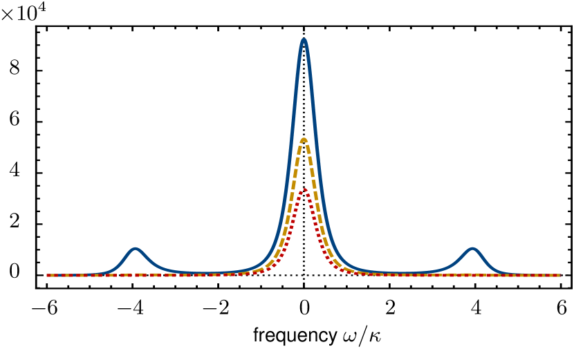
Figure 3: Exact optical output spectrum $\kappa S_{d^{\dagger}d}^{(0)}$ Eq. 32 (blue, solid) in comparison to a perfect BAE measurement of the modified mechanical spectrum (31) from Section IV.3 (yellow, dashed), and the RWA result Eq. 9 (red, dotted). The full spectrum (blue, solid) is calculated via Eq. 32, where additional terms due to the counterrotating quadrature $X_{-\delta}$ appear. The sidepeaks of the modified mechanical spectrum do not show in the yellow curve, as they are suppressed by $|\chi_{c}(\omega)|^{2}$. Parameters $\Gamma_{\text{eff}}/\kappa=1,\omega_{m}/\kappa=2,n_{\text{eff}}=10,G/\kappa=10,\delta=\omega_{m}$ (thus $\mathcal{C}=400$). Note that the large value of $\Gamma_{\text{eff}}$ is chosen for visibility.

As we have seen, CR terms modify the mechanical quadrature spectrum, which is reflected in the optical spectrum

$$S_{d^{\dagger}d}^{(0)}(\omega) =G^{2}|\chi_{c}(\omega)|^{2}\left[S_{xx}^{(0)}(\omega-\delta)+S_{xx}^{(0)}(\omega+\delta)\right.$$ (32)

$$\qquad\left.+S_{xx}^{(2)}(\omega-\delta)+S_{xx}^{(-2)}(\omega+\delta)\right]$$

$$=G^{2}|\chi_{c}(\omega)|^{2}\left[S_{X_{\delta}X_{\delta}}^{(0)}(\omega)+\lambda^{2}S_{X_{-\delta}X_{-\delta}}^{(0)}(\omega)\right.$$

$$\qquad\left.+\lambda\left(S_{X_{\delta}X_{-\delta}}^{(0)}(\omega)+S_{X_{-\delta}X_{\delta}}^{(0)}(\omega)\right)\right].$$

Comparing the second line of Eq. 32 to Eq. 9, we notice that there are extra terms present, namely those with at least one $\lambda$ out front. They are due to additional terms containing $X_{\delta}$ and $P_{\delta}$ on the RHS of the equation of motion for $Q$. In Fig. 2, they are denoted by the two gray arrows pointing to $Q$. Thus, this is an imperfection of the BAE measurement.

In fact, the additional contributions stem from the spectrum of the counterrotating quadrature $X_{-\delta}$ (i.e., with frequency $-\delta$) and correlations of that quadrature with $X_{\delta}$. That prompts a remarkably literal interpretation of “counterrotating terms”. It also clarifies the origin of the measurement BA. The CR quadrature can be written

$$X_{-\delta}(t)=\cos(2\delta t)X_{\delta}(t)+\sin(2\delta t)P_{\delta}(t),$$ (33)

which makes it apparent that the measurement picks up some information about $P_{\delta}$, the quadrature conjugate to $X_{\delta}$.

In contrast, the measurement backaction, as discussed in Section IV.3, arises from the gray arrows emanating from $I$. This correction is contained within $S_{X_{\delta}X_{\delta}}$ in Eq. 32.

In order to distinguish the two contributions (the imperfection and BA), we plot three functions in Fig. 3. The full optical spectrum (32) in blue (solid) encompasses both contributions. A perfect BAE measurement of the modified mechanical spectrum Eqs. 9 and 31 is shown in yellow (dashed), it picks up the thermal contribution and the BA. Finally, the expected result in RWA is red (dotted), which corresponds to a perfect BAE measurement of an otherwise undriven mechanical oscillator. The sidepeaks of the modified mechanical spectrum do not show in the yellow curve, as they are suppressed by $|\chi_{c}(\omega)|^{2}$.

IV.5 Mechanical and optical variances

An important application of BAE measurements is determining the quadrature variance, necessary for the verification of quantum squeezing. The BA imperils this by increasing the variance to

$$\expectationvalue{X_{\delta}^{2}}=\expectationvalue{X_{\text{RWA}}^{2}}+2n_{\text{CR}},$$ (34)

where $\expectationvalue{X_{\text{RWA}}^{2}}=\expectationvalue{X_{\text{unmeasured}}^{2}}$ is the result calculated without CR terms and (cf. (31))

$$2n_{\text{CR}}\equiv\int\frac{\differential\omega}{2\pi}S_{X_{\delta}X_{\delta}}^{\text{CR}}(\omega)=\frac{8G^{2}(\kappa/\Gamma_{\text{eff}}+1)}{(\Gamma_{\text{eff}}+\kappa)^{2}+16\omega_{m,\text{eff}}^{2}}.$$ (35)

Perhaps the most surprising aspect about this result is that $n_{\text{CR}}$ is independent of the temperature of the mechanical bath, whether it is squeezed or not, and what quadrature we measure. This fact is already realized on the level of the spectrum correction Eq. 31. The reason, as we have noted above, is that the optical quadrature $I$ in the measurement cavity is independent of the mechanics and that the BA is solely due to this quadrature (see Fig. 2). Note that although we have written the change in terms of a number of phonons $2n_{\text{CR}}$, it is not thermal heating that causes this effect, but rather the extraction of information about the conjugate quadrature.

In the optical spectrum, we saw that sidepeaks appear (cf. Fig. 3). To get an approximation to the variance of the measured mechanical quadrature, we integrate over the main peak of Eq. 32. Here, we calculate the error of this method, which can be used for underdamped oscillators $\Gamma_{\text{eff}}\ll\omega_{m,\text{eff}}$. The weight of the main peak is

$$\expectationvalue{X_{\text{meas}}^{2}}=\expectationvalue{X_{\text{RWA}}^{2}}+2n_{\text{CR}}\frac{16\omega_{m,\text{eff}}^{2}(2\Gamma_{\text{eff}}+\kappa)}{(\Gamma_{\text{eff}}+\kappa)(\Gamma_{\text{eff}}^{2}+16\omega_{m,\text{eff}}^{2})},$$ (36)

with $n_{\text{CR}}$ given by Eq. 35. It can be experimentally accessed by integrating $S_{d_{\text{out}}^{\dagger}d_{\text{out}}}^{(0)}(\omega)/(\kappa G^{2}|\chi_{c}(\omega)|^{2})$ from $-\omega_{m,\text{eff}}$ to $\omega_{m,\text{eff}}$, see Appendix E. The second term is the BA. For example, if $\Gamma_{\text{eff}}/\kappa=10^{-4}$, $G/\kappa=0.05$, and $\omega_{m}/\kappa=5$ (i.e., $\mathcal{C}=10^{6}$), the variance increases by $0.5$ (in units of the zero-point fluctuations of the mechanical oscillator). Since $n_{\text{CR}}\propto G^{2}$, stronger driving quickly makes this effect noticeable. In typical experimental regimes, where $\Gamma_{\text{eff}}\ll(\omega_{m},\kappa)$, the BA in Eq. 36 is well approximated by $2n_{\text{CR}}$, such that $\expectationvalue{X_{\text{meas}}^{2}}\approx\expectationvalue{X_{\delta}^{2}}$ (34), as desired.

Finally, we would like to gain some insights about the good and bad cavity limits of Eqs. 35 and 36. To give some intuition what these limits imply for the optical spectrum, consider the solution of Eq. 4a

$$d(t)=\int_{-\infty}^{t}\differential{\tau}e^{\frac{\kappa(\tau-t)}{2}}\left[2iG\cos(\omega_{m}\tau)x(\tau)+d_{\text{in}}(\tau)\right].$$ (37)

In the good cavity limit ($\omega_{m}\gg\kappa$), the exponential decay is negligible over a period $2\pi/\omega_{m}$. Thus

$$\int_{0}^{\frac{2\pi}{\omega_{m}}}\differential{\tau}\cos(\omega_{m}\tau)[\cos(\omega_{m}\tau)X_{\delta}(\tau)+\sin(\omega_{m}\tau)P_{\delta}(\tau)]\\ \approx(1/2)\int_{0}^{\frac{2\pi}{\omega_{m}}}\differential{\tau}X_{\delta}(\tau),$$ (38)

since $X_{\delta}(\omega)$ and $P_{\delta}(\omega)$ are centered around $\omega=0$. On the other hand, in the bad cavity limit $\kappa>\omega_{m}$ the photons leave the cavity faster than the change in coupling parameter, such that no averaging takes place. A simple argument then shows that the contribution from $X_{\delta}$ is roughly three times as big as the contribution from $P_{\delta}$.

These properties are reflected in the variances Eqs. 35 and 36. In the bad cavity limit, where $\kappa\gg\omega_{m,\text{eff}}$, the number of added phonons is

$$2n_{\text{CR}}\to\frac{8G^{2}}{\Gamma_{\text{eff}}(\Gamma_{\text{eff}}+\kappa)}.$$ (39)

In this regime the separation of the two drives is small compared to the bandwidth of the cavity, and therefore the BA becomes significant ($n_{\text{CR}}\sim 1$) at a cooperativity $\mathcal{C}\sim 1$, where $\mathcal{C}\equiv 4G^{2}/\kappa\Gamma_{\text{eff}}$. As we have seen, the reason is that resonant and CR terms couple with equal strength.

In contrast, the good cavity limit is $\kappa\gg\Gamma_{\text{eff}}$ and $\omega_{m,\text{eff}}\gg\kappa$, where Eq. 35 reduces to

$$2n_{\text{CR}}\to\frac{\kappa G^{2}}{2\Gamma_{\text{eff}}\omega_{m,\text{eff}}^{2}}.$$ (40)

This agrees with the perturbative result in Ref. Clerk et al. (2008). Equation 40 tells us that the BA depends inversely on the effective mechanical dissipation rate. Physically, this is because $\Gamma_{\text{eff}}$, the rate at which the mechanical oscillator relaxes to its steady state, competes with the BA rate due to CR terms, which is independent of $\Gamma_{\text{eff}}$. The BA also decreases with increasing $\omega_{m}$, as CR terms become less resonant. We find that the BA becomes significant ($n_{\text{CR}}\sim 1$) for a cooperativity $\mathcal{C}\sim 16\omega_{m}^{2}/\kappa^{2}$. Therefore, in the good cavity regime, the CR terms are suppressed by a factor ${\sim}16\omega_{m}^{2}/\kappa^{2}$ in comparison to resonant terms, due to the mechanism described above.

V Generalization

Above, we have taken $H_{\text{rest}}=0$ for simplicity, but we can in fact take any $H_{\text{rest}}$ and write down the solution, as long as we know the steady state of $H_{\text{OM}}+H_{\text{rest}}+H_{\text{baths}}$, i.e., without the BAE measurement ($G=0$). Furthermore, we need

$$[H_{\text{rest}},I]=0.$$ (41)

If the unmeasured solution is also periodic, the consideration in Malz and Nunnenkamp (2016) applies: For incommensurate periods, only the stationary part will be picked up by the measurement, but if they are commensurate, some other Fourier components may enter the output spectrum.

To formulate a general theory, we collect all system (input) operators into a vector $\vec{F}$ ($\vec{F}_{\text{in}}$). The Langevin equations read

$$\dot{\vec{F}}(t)=\bm{A}(t)\vec{F}(t)+\bm{L}\vec{F}_{\text{in}}(t).$$ (42)

For a time-independent $\bm{A}(t)=\bm{A}$, a Fourier transform yields

$$\vec{F}(\omega)=\bm{\chi}(\omega)\bm{L}\vec{F}_{\text{in}}(\omega),$$ (43)

with susceptibility matrix $\bm{\chi}(\omega)=(-i\omega-\bm{A})^{-1}$. We can do the same for a time-periodic $\bm{A}(t)=\bm{A}(t+T)$ once we have reformulated the problem in terms of Fourier components. Then

$$\vec{F}^{(n)}(\omega)=\sum_{m=-\infty}^{\infty}\bm{\chi}^{(n-m)}(\omega-n\delta)\bm{L}\vec{F}^{(m)}_{\text{in}}(\omega).$$ (44)

If we know how to solve the unmeasured system ($G=0$), we know how to find $\bm{\chi}^{(n)}$ in that case. Importantly, Eq. 44 does not make any assumption about the noise $\vec{F}_{\text{in}}^{(n)}$, apart from stationarity. For this reason, the replacement in Eq. 24 above will leave the susceptibility matrix $\bm{\chi}^{(n)}(\omega)$ unchanged and therefore can be used to calculate the measurement BA for all systems with suitable $H_{\text{rest}}$. In the end, we can write down the scattering matrix in terms of the susceptibility matrix

$$\bm{S}^{(n)}(\omega)=\delta_{0,n}\bm{1}-\bm{L}\bm{\chi}^{(n)}(\omega)\bm{L},$$ (45)

which can be use to calculate the output fields

$$\vec{F}_{\text{out}}^{(n)}(\omega)=\sum_{m}\bm{S}^{(n-m)}(\omega-n\delta)\vec{F}_{\text{in}}^{(m)}(\omega).$$ (46)

For examples how $\bm{\chi}$ can look like, see the detailed calculations in Appendices B, A, C and D. Appendix A contains the setup used to produce bichromatic squeezing Mari and Eisert (2009); Kronwald et al. (2013); Lecocq et al. (2015); Pirkkalainen et al. (2015); Wollman et al. (2015); Malz and Nunnenkamp (2016); Lei et al. (2016), Appendix B discusses a weak-coupling version of the former, which is easily adapted to other weakly coupled systems, and Appendix C contains the parametric squeezing case, which is an example with more than one independent, relevant component in $\bm{\chi}$. Last is Appendix D, which extends the method here to two mechanical modes, and covers a recently developed two-mode BAE measurement Woolley and Clerk (2013); Ockeloen-Korppi et al. (2016).

VI Conclusion

Using the framework from Ref. Malz and Nunnenkamp (2016), we derived the full solution of an optomechanical system subject to a dual-beam BAE measurement Bocko and Onofrio (1996); Hertzberg et al. (2010); Suh et al. (2014); Lecocq et al. (2015); Lei et al. (2016). This enables us to calculate the modification of the spectrum and quantify the measurement backaction precisely. Furthermore, we demonstrate that our technique is versatile, by showing how to generalize the calculation to systems where the mechanical resonator is additionally coupled to other degrees of freedom and illustrate the technique with several examples.

Appendix A Dissipative bichromatic squeezing

An important application of the type of BAE measurement discussed in this article is the verification of quantum squeezing in mechanical resonators, e.g., Refs. Lecocq et al. (2015); Lei et al. (2016). Here we generalize our method to this squeezing scheme, proposed in Mari and Eisert (2009); Kronwald et al. (2013), which has successfully produced quantum squeezing of the resonator Wollman et al. (2015); Pirkkalainen et al. (2015); Lecocq et al. (2015); Lei et al. (2016). In this case

$$H_{\text{rest}}=-\Delta c^{\dagger}c-\left[c\left(G_{+}e^{2i\delta t}b+G_{-}b^{\dagger}\right)+\text{h.c.}\right],$$ (47)

where we have already displaced and linearized. $c$ is the annihilation operator of another cavity in a frame rotating with the lower-frequency drive. Furthermore, we have applied the RWA to $H_{\text{rest}}$. The governing Langevin equations are

$$\dot{c} =\left(i\Delta-\frac{\kappa_{2}}{2}\right)c+\sqrt{\kappa_{2}}c_{\text{in}}+i\left(G_{-}b+G_{+}e^{-2i\delta t}b^{\dagger}\right),$$ (48a)

$$\dot{b} =\left(-i\omega_{m}-\frac{\gamma}{2}\right)b+\sqrt{\gamma}b_{\text{in}}+i\left(G_{-}c+G_{+}e^{-2i\delta t}c^{\dagger}\right),$$ (48b)

where $c_{\text{in}}$ corresponds to a vacuum (zero temperature) bath, and $b_{\text{in}}$ to a finite temperature bath with mean occupation $n_{\text{th}}$, so $\expectationvalue{c_{\text{in}}(t)c_{\text{in}}(t^{\prime})^{\dagger}}=\delta(t-t^{\prime})$, $\expectationvalue{b_{\text{in}}(t)^{\dagger}b_{\text{in}}(t^{\prime})}=\delta(t-t^{\prime})n_{\text{th}}$, $\expectationvalue{b_{\text{in}}(t)b_{\text{in}}(t^{\prime})^{\dagger}}=\delta(t-t^{\prime})(1+n_{\text{th}})$ (other correlators are zero).

In the Floquet ansatz, Eq. 48 can be expressed in terms of a block-diagonal infinite matrix Malz and Nunnenkamp (2016) with blocks

$$\begin{pmatrix}\chi_{\text{opt}}^{-1}(\omega-n\delta)&-iG_{-}&0&-iG_{+}\\ -iG_{-}&\chi_{m}^{-1}(\omega-n\delta)&-iG_{+}&0\\ 0&iG_{+}&\chi_{\text{opt}}^{-1*}(-\omega+(n+2)\delta)&iG_{-}\\ iG_{+}&0&iG_{-}&\chi_{m}^{-1*}(-\omega+(n+2)\delta)\end{pmatrix}\begin{pmatrix}c^{(n)}(\omega)\\ b^{(n)}(\omega)\\ c^{(n+2){\dagger}}(\omega)\\ b^{(n+2){\dagger}}(\omega)\end{pmatrix}=\begin{pmatrix}\sqrt{\kappa}c_{\text{in}}^{(n)}(\omega)\\ \sqrt{\gamma}b_{\text{in}}^{(n)}(\omega)\\ \sqrt{\kappa}c_{\text{in}}^{(n+2){\dagger}}(\omega)\\ \sqrt{\gamma}b_{\text{in}}^{(n+2){\dagger}}(\omega)\end{pmatrix},$$ (49)

where the cavity and mechanical response functions read $\chi_{\text{opt}}(\omega)=[\kappa/2-i(\omega+\Delta)]^{-1}\neq\chi_{c}$ and $\chi_{m}(\omega)=[\gamma/2-i(\omega-\omega_{m})]^{-1}$, respectively.

Blocks with zero input will vanish in the steady state. Since the noise resides entirely in the zeroth Fourier component (it describes a stationary process),

$$c_{\text{in}}^{(n)}=b_{\text{in}}^{(n)}=0,\qquad\forall n\neq 0.$$ (50)

Although the result for general $\delta$ and $\Delta$ is available Malz and Nunnenkamp (2016), we focus on the simple and relevant case $\delta=-\Delta=\omega_{m}$, where

$$\begin{pmatrix}b^{(0)}(\omega)\\ b^{(2){\dagger}}(\omega)\end{pmatrix}=J(\omega)\begin{pmatrix}1&iG_{-}\chi_{\text{opt}}(\omega)\\ 0&iG_{+}\chi_{\text{opt}}(\omega)\end{pmatrix}\begin{pmatrix}\sqrt{\gamma}b_{\text{in}}\\ \sqrt{\kappa_{2}}c_{\text{in}}\end{pmatrix},$$ (51)

with $J(\omega)=\left[\chi_{m}^{-1}(\omega)+\mathcal{G}^{2}\chi_{\text{opt}}(\omega)\right]^{-1}.$

Now we include the noise of a BAE measurement as per Section V. The measurement requires another cavity mode coupled to the mechanical oscillator. We define

$$\vec{F}=\begin{pmatrix}b&b^{\dagger}&c&c^{\dagger}\end{pmatrix},\quad\vec{F}_{\text{in}}=\begin{pmatrix}b_{\text{in}}&b_{\text{in}}^{\dagger}&c_{\text{in}}&c_{\text{in}}^{\dagger}\end{pmatrix}.$$ (52)

From Eq. 51, we can directly infer the elements

$$\begin{pmatrix}\bm{\chi}_{11}^{(0)}(\omega)&\bm{\chi}_{13}^{(0)}(\omega)\\ \bm{\chi}_{21}^{(2)}(\omega-2\delta)&\bm{\chi}_{23}^{(2)}(\omega-2\delta)\end{pmatrix}=J(\omega)\begin{pmatrix}1&iG_{-}\chi_{\text{opt}}(\omega)\\ 0&iG_{+}\chi_{\text{opt}}(\omega)\end{pmatrix}.$$ (53)

Furthermore, the elements of $\bm{\chi}$ are not all independent. In general,

$$\chi_{ij}^{(n)*}(\omega)=\chi_{\bar{i}\bar{j}}^{(-n)}(-\omega),$$ (54)

where $\bar{i}$ is the index for the operator that is the hermitian conjugate of the operator indexed by $i$ (so $\bar{1}=2$, $\bar{3}=4$, and vice versa).

We are only interested in the elements that connect the system operators with the mechanical bath, as those will determine the susceptibility to the measurement noise. Fortunately, the only non-zero ones are

$$\bm{\chi}_{11}^{(0)}(\omega)=J(\omega)=\bm{\chi}_{22}^{(0)*}(-\omega).$$ (55)

This gives the problem exactly the same structure as the case with $H_{\text{rest}}=0$, except that here $\chi_{m}(\omega)$ is replaced by $J(\omega)$.

Nevertheless, we give the general formula for the added contribution due to the measurement

$$b_{\text{add}}^{(n)}(\omega) =2\sqrt{\kappa}G\sum_{m}K^{(n-m)}(\omega-n\delta)f_{\text{in}}^{(m)}(\omega),$$ (56a)

$$b_{\text{add}}^{(n){\dagger}}(\omega) =2\sqrt{\kappa}G\sum_{m}K^{(-n+m)*}(-\omega+n\delta)f_{\text{in}}^{(m)}(\omega),$$ (56b)

where

$$K^{(n)}(\omega)\equiv\bm{\chi}_{11}^{(n)}(\omega)-\bm{\chi}_{12}^{(n)}(\omega).$$ (57)

This gives (note similarity with Eq. 19)

$$b^{(n)}_{\text{add}}=2\sqrt{\kappa}GJ(\omega-n\delta)f_{\text{in}}^{(n)}(\omega).$$ (58)

and hermitian conjugate. The CR correction can be calculated as before and looks very familiar (cf. Eq. 31)

$$S_{X_{\delta}X_{\delta}}^{\text{CR}}(\omega)=\kappa\lambda^{2}G^{2}\left(|J(\omega+\delta)\chi_{c}(\omega+2\delta)|^{2}\right.\\ \left.+|J(-\omega+\delta)\chi_{c}(-\omega+2\delta)|^{2}\right).$$ (59)

The reason why it is so simple is that here $b^{(0)}(\omega)$ only couples to $b_{\text{in}}$ and not to $b_{\text{in}}^{\dagger}$. This ceases to be the case for $\Delta\neq-\omega_{m}$, or in parametric squeezing in Appendix C.

Appendix B Dissipative bichromatic squeezing in the absence of strong-coupling effects

As a relevant example for how a weakly coupled $H_{\text{rest}}$ can lead to effective parameters in the mechanical susceptibility, we consider the weak-coupling version of Appendix A. We place the red-detuned drive on the red sideband $\Delta=-\omega_{m}$, but allow the other to vary. To second order in $G_{\pm}$, the effective quantum Langevin equation is (in a frame rotating with frequency $\delta$)

$$\dot{b}=-\left[i(\omega_{m,\text{eff}}-\delta)+\frac{\Gamma_{\text{eff}}}{2}\right]b+\sqrt{\gamma}b_{\text{in}}+\frac{2i\mathcal{G}}{\sqrt{\kappa}}s_{\text{in}},$$ (60)

with Malz and Nunnenkamp (2016)

$$\Gamma_{\text{eff}} =\gamma+\frac{4}{\kappa}\left(G_{-}^{2}-\frac{G_{+}^{2}}{1+4\varepsilon^{2}/\kappa^{2}}\right),$$ (61a)

$$\omega_{m,\text{eff}} =\omega_{m}+\frac{G_{+}^{2}\varepsilon}{(\kappa/2)^{2}+\varepsilon^{2}},$$ (61b)

$$s_{\text{in}} =\frac{G_{-}d_{\text{in}}+G_{+}d_{\text{in}}^{\dagger}}{\mathcal{G}}.$$ (61c)

Here, $\varepsilon\equiv 2(\delta-\omega_{m})$ and $\mathcal{G}\equiv\sqrt{G_{-}^{2}-G_{+}^{2}}$. $s_{\text{in}}$ is a Bogoliubov rotation of the original optical bath operators, and is therefore a squeezed, vacuum bath with nonzero anomalous correlators, such as $\expectationvalue{s_{\text{in}}(\omega)s_{\text{in}}(\omega^{\prime})}=-2\pi\delta(\omega+\omega^{\prime})G_{+}G_{-}/\mathcal{G}^{2}$.

The equivalent master equation (generalization of Ref. Kronwald et al. (2013) to general drive detuning $\delta$) is

$$\dot{\rho}=-i[(\omega_{m,\text{eff}}-\delta)b^{\dagger}b,{\rho}]+\left\{\Gamma_{\text{eff}}(n_{\text{eff}}+1)\mathcal{D}[b]\right.\\ \left.+\Gamma_{\text{eff}}n_{\text{eff}}\mathcal{D}[b^{\dagger}]+\frac{4\mathcal{G}^{2}}{\kappa}\mathcal{D}[\beta]\right\}{\rho},$$ (62)

where $\mathcal{D}[a]{\rho}\equiv a{\rho}a^{\dagger}-\frac{1}{2}(a^{\dagger}a{\rho}+{\rho}a^{\dagger}a)$ is the Lindblad superoperator.

In order to include the measurement noise, it is easier to work in the laboratory frame, where

$$\dot{b}=-\left(i\omega_{m,\text{eff}}+\frac{\Gamma_{\text{eff}}}{2}\right)b+\sqrt{\gamma}b_{\text{in}}+2\sqrt{\kappa}Gf_{\text{in}}+\frac{2i\mathcal{G}}{\sqrt{\kappa}}s_{\text{in}}.$$ (63)

There is a subtlety here, as the anomalous averages of $s_{\text{in}}$, will become rotating in the transition from a rotating frame into the laboratory frame. We can ignore this difficulty, because we are only interested in the correction. Rewriting Eq. 63 in Fourier components, we find that the only independent nonzero element of the susceptibility matrix is

$$\bm{\chi}_{11}^{(0)}(\omega)=\chi_{m,\text{eff}}(\omega)\equiv[\Gamma_{\text{eff}}/2-i(\omega-\omega_{m,\text{eff}})]^{-1}.$$ (64)

We could have obtained this from Eq. 55 by setting $\mathcal{G}=0$ (weak coupling) and replacing $\omega_{m}$ and $\gamma$ by their modified values. Thus we can use the result Eq. 59 with $J\to\chi_{m,\text{eff}}$. Therefore, the results in the article are valid in the weak coupling case as well, with $\gamma\to\Gamma_{\text{eff}}$ and $\omega_{m}\to\omega_{m,\text{eff}}$.

Optionally, we can remain in a rotating frame, but that means we have to rotate the added measurement noise to $\tilde{f}_{\text{in}}\equiv e^{i\delta t}f_{\text{in}}$. This implies $\tilde{f}_{\text{in}}^{(n)}=f_{\text{in}}^{(n-1)}$. Solving the Langevin equation gives $\chi_{11}^{(0)}(\omega)=[\Gamma_{\text{eff}}/2-i(\omega-\omega_{m,\text{eff}}+\delta)]^{-1}$. Consulting Eq. 56, we find that the new set of Fourier components $\tilde{b}_{\text{add}}^{(n)}(\omega)=b_{\text{add}}^{(n-1)}(\omega)$. It is straightforward to check that in the end $\tilde{b}_{\text{add}}(t)=e^{i\delta t}b_{\text{add}}(t)$.

This result can be adapted to a wide variety of cases, as long as they can be approximated by coupling the harmonic oscillators to baths only (and potentially modify its effective parameters).

Appendix C Parametric squeezing

Squeezing is induced naturally in a degenerate parametric amplifier Walls and Milburn (2008). Whilst it is limited to 3 dB of squeezing, its solution has other interesting aspects. Here,

$$H_{\text{rest}}=\omega_{m}b^{\dagger}b+(\mu b^{2}e^{2i\omega_{m}t}+\text{h.c.}),$$ (65)

where $\mu$ is the parametric driving strength. Without the BAE measurement $(G=0$), the quantum Langevin equation is

$$\dot{b}=-i\omega_{m}b-i\mu b^{\dagger}e^{-2i\omega_{m}t}-\frac{\gamma}{2}b+\sqrt{\gamma}b_{\text{in}}.$$ (66)

In Fourier components,

$$\begin{pmatrix}\chi_{m}^{-1}(\omega-n\omega_{m})&i\mu\\ -i\mu&\chi_{m}^{-1}(\omega-n\omega_{m})\end{pmatrix}\begin{pmatrix}b^{(n)}(\omega)\\ b^{(n+2){\dagger}}(\omega)\end{pmatrix}\\ =\sqrt{\gamma}\begin{pmatrix}\delta_{n,0}b_{\text{in}}\\ \delta_{n,2}b_{\text{in}}^{\dagger}\end{pmatrix},$$ (67)

where $\chi_{m}(\omega)\equiv\left[\gamma/2-i(\omega-\omega_{m})\right]^{-1}$. Inverting leads to

$$\begin{pmatrix}b^{(n)}(\omega)\\ b^{(n+2){\dagger}}(\omega)\end{pmatrix}=A(\omega-n\omega_{m})\\ \times\begin{pmatrix}\chi_{m}^{-1}(\omega-n\omega_{m})&-i\mu\\ i\mu&\chi_{m}^{-1}(\omega-n\omega_{m})\end{pmatrix}\begin{pmatrix}\sqrt{\gamma}\delta_{n,0}b_{\text{in}}\\ \sqrt{\gamma}\delta_{n,2}b_{\text{in}}^{\dagger}\end{pmatrix},$$ (68)

where

$$A(\omega)\equiv\left[\chi_{m}^{-2}(\omega-n\omega_{m})-\mu^{2}\right]^{-1}.$$ (69)

It is again enough to consider only one block (the other nonzero block is the hermitian conjugate)

$$\begin{pmatrix}b^{(0)}(\omega)\\ b^{(2){\dagger}}(\omega)\end{pmatrix}=A(\omega)\begin{pmatrix}\chi_{m}^{-1}(\omega)&-i\mu\\ i\mu&\chi_{m}^{-1}(\omega)\end{pmatrix}\begin{pmatrix}\sqrt{\gamma}b_{\text{in}}\\ 0\end{pmatrix}.$$ (70)

To make the discussion as simple as possible, we choose $\delta=\omega_{m}$ for the measurement scheme. Then the same analysis as above can be applied to obtain

$$\bm{\chi}^{(0)}_{11}(\omega) =A(\omega)\chi_{m}^{-1}(\omega),$$ (71a)

$$\bm{\chi}^{(2)}_{12}(\omega-2\omega_{m}) =-i\mu A(\omega),$$ (71b)

$$\bm{\chi}^{(-2)*}_{12}(-\omega+2\omega_{m}) =i\mu A^{*}(\omega).$$ (71c)

In order to evaluate the added noise due to the BAE measurement, we have to add the noise Eq. 20 and use Eq. 56. We find ($\lambda$ labels terms with CR origin)

$$b_{\text{add}}^{(n)} (\omega)=i\sqrt{\kappa}G\chi_{c}(\omega)I_{\text{in}}(\omega)$$ (72)

$$\times\begin{cases}i\mu A(\omega-\delta)&\text{if }n=3\\ i\mu\lambda A(\omega+\delta)+A(\omega-\delta)\chi_{m}^{-1}(\omega-\delta)&\text{if }n=1\\ \lambda A(\omega+\delta)\chi_{m}^{-1}(\omega+\delta)&\text{if }n=-1\end{cases}$$

This reverts to Eq. 19 when we set $\mu=0$. Using Eq. 28 with the spectra calculated from Eq. 72, we obtain the correction to the quadrature spectrum. The resulting spectra have terms rotating at multiples of $\delta$. They could be measured by coupling to another suitably driven cavity mode Malz and Nunnenkamp (2016), but tend to be very small.

Appendix D Two-mode BAE

In this section, we consider another recently experimentally demonstrated QND scheme Woolley and Clerk (2013); Ockeloen-Korppi et al. (2016). The goal here is to measure a collective quadrature of two mechanical oscillators, in order to eventually measure both quadratures of an external force with the same device. Whilst the overall theory is more general Tsang and Caves (2012), in the specific experiment we consider here, both mechanical resonators couple to the same cavity and the problem has the Hamiltonian Woolley and Clerk (2013)

$$H =(\omega_{m}+\Omega)b_{1}^{\dagger}b_{1}+(\omega_{m}-\Omega)b_{2}^{\dagger}b_{2}+\omega_{\text{cav}}a^{\dagger}a$$ (73)

$$+g_{1}(b_{1}+b_{1}^{\dagger})a^{\dagger}a+g_{2}(b_{2}+b_{2}^{\dagger})a^{\dagger}a+H_{\text{drive}}+H_{\text{diss}}$$

Note that in Ref. Woolley and Clerk (2013) the mechanical oscillators have annihilation operators $a$ and $b$, and the cavity $c$, whereas here, they are $b_{1},b_{2}$, and $a$, respectively. As before, bichromatic driving leads to a coherent state

$$\hat{a}=2\cos(\Omega t)\bar{a}+\hat{d},$$ (74)

where $\bar{a}$ is a real number, and $\langle\hat{d}\rangle=0$.

Our generic solution is applicable, because Eq. 41 is fulfilled after linearizing, no matter which of the oscillators we put into $H_{\text{rest}}$. For example, we could chose

$$H_{\text{rest,1}}=(\omega_{m}+\Omega)b_{1}^{\dagger}b_{1}+g_{1}(b_{1}+b_{1}^{\dagger})2\cos(\Omega t)\bar{a}(d+d^{\dagger}),$$ (75)

but the choice with $1\to 2$ is equally valid. Our result for the backaction on the mechanical oscillators (all of Section IV, particularly Eq. 31) thus applies to both resonators individually.

The correction to the cavity spectrum is slightly more tricky to find, since the fluctuations in the two resonators are correlated, leading to cross terms. Instead of Eq. 4a we have

$$\dot{d}=-\frac{\kappa}{2}d+\sqrt{\kappa}d_{\text{in}}+2i\cos(\Omega t)\left(G_{1}x_{1}+G_{2}x_{2}\right),$$ (76)

where $x_{1,2}$ are the position operators for the two oscillators, and $G_{1,2}\equiv g_{1,2}\bar{a}$. $x_{1,2}$ are both given through Eq. 19, but with the respective parameters for each resonator.

To calculate the optical spectrum, first note that there is a cross correlation. For $m,n\in\{1,-1\}$, we have

$$\int\frac{\differential{\omega^{\prime}}}{2\pi}\expectationvalue{x_{1}^{(m)}(\omega+m\delta)x_{2}^{(n)}(\omega^{\prime})}=-\kappa G_{1}G_{2}$$ (77)

$$\times|\chi_{c}(\omega+m\delta)|^{2}\chi_{x_{1}}(\omega)\chi_{x_{2}}(-\omega-(m+n)\delta),$$

with $\chi_{x_{1,2}}$ defined analogously to $\chi_{x}$ in Appendix G. Then $S_{d^{\dagger}d}^{(0)}$ contains two copies of Eq. 32 (one for each resonator), in addition to

$$4G^{2}|\chi_{c}(\omega)|^{2}\mathrm{Re}\left[S_{x_{1}x_{2}}^{(0)}(\omega-\delta)+S_{x_{1}x_{2}}^{(0)}(\omega+\delta)\right.$$ (78)

$$\qquad+\left.S_{x_{1}x_{2}}^{(2)}(\omega-\delta)+S_{x_{1}x_{2}}^{(-2)}(\omega+\delta)\right],$$

where $S_{x_{1}x_{2}}$ are given through Eqs. 16 and 77. Here, we used the property $[S_{AB}^{(n)}(\omega)]^{\dagger}=S_{B^{\dagger}A^{\dagger}}^{(-n)}(\omega+n\delta)$ Malz and Nunnenkamp (2016).

This demonstrates that our technique can also be applied for multiple modes coupled to the cavity, as long as $[H_{\text{rest}},I]=0$.

Appendix E Integration of the main peak

One goal of a BAE measurement of a mechanical oscillator quadrature is to extract the quadrature variance. We show that the weight of the main peak of the optical spectrum

$$\frac{S_{d^{\dagger}d}^{(0)}(\omega)}{G^{2}|\chi_{c}(\omega)|^{2}}=S_{xx}^{(0)}(\omega-\delta)+S_{xx}^{(0)}(\omega+\delta)$$ (79)

$$\qquad+S_{xx}^{(2)}(\omega-\delta)+S_{xx}^{(-2)}(\omega+\delta)$$

is a good measure for the quadrature variance. The weight of its middle peak at $\omega=0$ is

$$W=\int_{-\infty}^{\infty}\frac{\differential{\omega}}{2\pi}S_{xx}^{(0)}(\omega)+2\mathrm{Re}[S_{xx}^{(2)}(\omega)].$$ (80)

Equation 80 can be evaluated with the formulae in Appendix G. Given the output spectrum $\kappa S_{d^{\dagger}d}^{(0)}(\omega)$, the weight can be approximated by integrating from $-\omega_{m}$ to $\omega_{m}$

$$W\approx\expectationvalue{X_{\text{meas}}^{2}}\equiv\int_{-\omega_{m}}^{\omega_{m}}\frac{\differential{\omega}}{2\pi}\frac{S_{d_{\text{out}}^{\dagger}d_{\text{out}}}^{(0)}(\omega)}{\kappa G^{2}|\chi_{c}(\omega)|^{2}}.$$ (81)

Appendix F Full quadrature spectrum

Here we present the full expression for the spectrum of the rotating quadrature $X_{\delta}$

$$S_{X_{\delta}X_{\delta}}^{(0)}(\omega) =\gamma\left(|\chi_{m}(\omega+\delta)|^{2}(n_{\text{th}}+1)+|\chi_{m}(-\omega+\delta)|^{2}n_{\text{th}}\right)+\kappa G^{2}\left\{-2|\chi_{c}(\omega)|^{2}\mathrm{Re}\left[\chi_{m}(\omega+\delta)\chi_{m}(-\omega+\delta)\right]\right.$$ (82)

$$+\left.|\chi_{m}(\omega+\delta)|^{2}\left(|\chi_{c}(\omega)|^{2}+|\chi_{c}(\omega+2\delta)|^{2}\right)+|\chi_{m}(-\omega+\delta)|^{2}\left(|\chi_{c}(\omega-2\delta)|^{2}+|\chi_{c}(\omega)|^{2}\right)\right\}.$$

It contains a part due to the thermal bath of the oscillator (terms with a $\gamma$) and an optical part (terms with $\kappa$). If $\delta=\omega_{m}$, $\chi_{m}(-\omega+\delta)=\chi_{m}^{*}(\omega+\delta)$, and the negative term in the curly brackets cancels two resonant contributions in the second line. This cancellation makes the measurement BAE in RWA. The two terms left over cause the two side peaks to appear. Inverting the sign of the first term in curly brackets would lead to the spectrum of the conjugate quadrature $S_{P_{\delta}P_{\delta}}^{(0)}(\omega)$, which gets all the BA in RWA. The BA due to CR terms is the same in both. If the oscillator is weakly coupled to other degrees of freedom, this formula is still approximately correct, using effective parameters $\Gamma_{\text{eff}}$, $\omega_{m,\text{eff}}$ and $n_{\text{eff}}$.

Appendix G Optical spectrum

In this section we outline the derivation of the optical spectrum. We use the expression given in the main text (32). For $H_{\text{rest}}=0$, the necessary correlators are

$$\int\frac{\differential{\omega^{\prime}}}{2\pi}\expectationvalue{x^{(0)}(\omega)x^{(0)}(\omega^{\prime})}=\gamma\left[|\chi_{m}(-\omega)|^{2}n_{\text{th}}+|\chi_{m}(\omega)|^{2}(n_{\text{th}}+1)\right],$$ (83)

and for $m,n\in\{1,-1\}$

$$\int\frac{\differential{\omega^{\prime}}}{2\pi}\expectationvalue{x^{(m)}(\omega+m\delta)x^{(n)}(\omega^{\prime})}=-\kappa G^{2}|\chi_{c}(\omega+m\delta)|^{2}\chi_{x}(\omega)\chi_{x}(-\omega-(m+n)\delta),$$ (84)

where $\chi_{x}(\omega)\equiv\chi_{m}(\omega)-\lambda\chi_{m}^{*}(-\omega).$ This gives

$$S_{xx}^{(0)}(\omega) =\gamma\left[|\chi_{m}(-\omega)|^{2}n_{\text{th}}+|\chi_{m}(\omega)|^{2}(n_{\text{th}}+1)\right]+\kappa G^{2}\left(|\chi_{x}(-\omega)|^{2}|\chi_{c}(\omega+\delta)|^{2}+|\chi_{x}(\omega)|^{2}|\chi_{c}(\omega-\delta)|^{2}\right),$$ (85a)

$$S_{xx}^{(2)}(\omega) =-\kappa G^{2}|\chi_{c}(\omega+\delta)|^{2}\chi_{x}^{*}(-\omega)\chi_{x}^{*}(\omega+2\delta),$$ (85b)

$$S_{xx}^{(-2)}(\omega) =-\kappa G^{2}|\chi_{c}(\omega-\delta)|^{2}\chi_{x}(\omega)\chi_{x}(-\omega+2\delta),$$ (85c)

whence $S_{d^{\dagger}d}^{(0)}(\omega)$ can be constructed, using (cf. Eq. 32)

$$S_{d^{\dagger}d}^{(n)}(\omega)=G^{2}\chi_{c}(\omega)\chi_{c}^{*}(\omega+n\delta)\left[S_{xx}^{(n)}(\omega-\delta)+S_{xx}^{(n)}(\omega+\delta)+S_{xx}^{(n+2)}(\omega-\delta)+S_{xx}^{(n-2)}(\omega+\delta)\right].$$ (86)

References

- Caves et al. (1980) C. M. Caves, K. S. Thorne, R. W. P. Drever, V. D. Sandberg, and M. Zimmermann, Reviews of Modern Physics 52, 341 (1980).
- Clerk et al. (2010) A. A. Clerk, M. H. Devoret, S. M. Girvin, F. Marquardt, and R. J. Schoelkopf, Reviews of Modern Physics 82, 1155 (2010).
- Braginsky et al. (1980) V. B. Braginsky, Y. I. Vorontsov, and K. S. Thorne, Science 209, 547 (1980).
- Abbott and Others (2016) B. P. Abbott and Others, Physical Review Letters 116, 061102 (2016), arXiv:1602.03837 .
- Bocko and Onofrio (1996) M. F. Bocko and R. Onofrio, Reviews of Modern Physics 68, 755 (1996).
- Clerk et al. (2008) A. A. Clerk, F. Marquardt, and K. Jacobs, New Journal of Physics 10, 095010 (2008), arXiv:0802.1842 .
- Hertzberg et al. (2010) J. B. Hertzberg, T. Rocheleau, T. Ndukum, M. Savva, A. A. Clerk, and K. C. Schwab, Nature Physics 6, 213 (2010).
- Suh et al. (2014) J. Suh, A. J. Weinstein, C. U. Lei, E. E. Wollman, S. K. Steinke, P. Meystre, A. A. Clerk, and K. C. Schwab, Science 344, 1262 (2014), arXiv:1312.4084 .
- Lecocq et al. (2015) F. Lecocq, J. B. Clark, R. W. Simmonds, J. Aumentado, and J. D. Teufel, Physical Review X 5, 041037 (2015), arXiv:1509.01629v1 .
- Lei et al. (2016) C. U. Lei, A. J. Weinstein, J. Suh, E. E. Wollman, A. Kronwald, F. Marquardt, A. A. Clerk, and K. C. Schwab, Physical Review Letters 117, 100801 (2016), arXiv:1605.08148 .
- Polzik and Hammerer (2014) E. S. Polzik and K. Hammerer, Annalen der Physik 527, A15 (2014), arXiv:1405.3067 .
- Malz and Nunnenkamp (2016) D. Malz and A. Nunnenkamp, Physical Review A 94, 023803 (2016), arXiv:1605.04749 .
- Aspelmeyer et al. (2014) M. Aspelmeyer, T. J. Kippenberg, and F. Marquardt, Reviews of Modern Physics 86, 1391 (2014).
- Gardiner and Zoller (2004) C. Gardiner and P. Zoller, Quantum Noise: A Handbook of Markovian and Non-Markovian Quantum Stochastic Methods with Applications to Quantum Optics, Springer Series in Synergetics (Springer, 2004).
- Weinstein et al. (2014) A. J. Weinstein, C. U. Lei, E. E. Wollman, J. Suh, A. Metelmann, A. A. Clerk, and K. C. Schwab, Physical Review X 4, 041003 (2014), arXiv:1404.3242 .
- Mari and Eisert (2009) A. Mari and J. Eisert, Physical Review Letters 103, 213603 (2009), arXiv:0911.0433 .
- Kronwald et al. (2013) A. Kronwald, F. Marquardt, and A. A. Clerk, Physical Review A 88, 063833 (2013).
- Pirkkalainen et al. (2015) J.-M. Pirkkalainen, E. Damskägg, M. Brandt, F. Massel, and M. A. Sillanpää, Physical Review Letters 115, 243601 (2015), arXiv:1507.04209 .
- Wollman et al. (2015) E. E. Wollman, C. U. Lei, A. J. Weinstein, J. Suh, A. Kronwald, F. Marquardt, A. A. Clerk, and K. C. Schwab, Science 349, 952 (2015), arXiv:1507.01662 .
- Woolley and Clerk (2013) M. J. Woolley and A. A. Clerk, Physical Review A 87, 063846 (2013), arXiv:1304.4059 .
- Ockeloen-Korppi et al. (2016) C. F. Ockeloen-Korppi, E. Damskägg, J.-M. Pirkkalainen, A. A. Clerk, M. J. Woolley, and M. A. Sillanpää, Physical Review Letters 117, 140401 (2016).
- Walls and Milburn (2008) D. Walls and G. J. Milburn, Quantum Optics, edited by D. Walls and G. J. Milburn (Springer Berlin Heidelberg, Berlin, Heidelberg, 2008).
- Tsang and Caves (2012) M. Tsang and C. M. Caves, Physical Review X 2, 031016 (2012).