Data-Unit-Size Distribution Model with Retransmitted Packet Size Preservation Property and Its Application to Goodput Analysis for Stop-and-Wait Protocol: Case of Independent Packet Losses

Abstract

This paper proposes a data-unit-size distribution model to represent the retransmitted packet size preservation (RPSP) property in a scenario where independently lost packets are retransmitted by a stop-and-wait protocol. RPSP means that retransmitted packets with the same sequence number are equal in size to the packet of the original transmission, which is identical to the packet generated from a message through the segmentation function, namely, generated packet. Furthermore, we derive goodput formula using an approach to derive the data-unit-size distribution. We investigate the effect of RPSP on frame size distributions and goodput in a simple case when no collision happens over the bit-error prone wireless network equipped with IEEE 802.11 Distributed Coordination Function, which is a typical example of the stop-and-wait protocol. Numerical results show that the effect gets stronger as bit error rate increases and the maximum size of the generated packets is larger than the mean size for large enough packet retry limits because longer packets will be repeatedly corrupted and retransmitted more times as a result of RPSP.

I Introduction

Transfers of data units over communication networks suffer frequently from failure due to various reasons including bit errors, congestion and collision. To provide an error-free transmission service of messages, i.e., data units generated by reliable applications, a sender requires to implement one or more communication protocols that include error recovery function. The error recovery function allows the sender to retransmit lost packets. For example, distributed coordination function (DCF) for IEEE 802.11 wireless local area networks specifies a stop-and-wait protocol (SWP) to realize the error-recovery function in a simple manner [1].

The packets, i.e., SWP-layer data units, that have been corrupted or lost within the networks will be transmitted by the error-recovery function. In general, such retransmitted packets with the same sequence number (seqNum) are equal in size to the packet in the original transmission. We call this property retransmitted packet size preservation: RPSP.

The packet retransmission probability will depend on the size of frames, which are data units that contain the packet and are transferred over physical links. Typical situations include the case when frames are lost due to bit errors because the frame corruption probability is approximately proportional to the frame size.

In papers [2, 3, 4], the effect of RPSP on the mean frame size was discussed for bit error prone networks. These papers showed that the mean frame size with RPSP is larger than that without RPSP as bit error rate increase if the packet size distribution has dispersion. The reason for this is that longer frames will be repeated corrupted more time due to RPSP.

The frame sizes affect several quality of service (QoS) parameters (e.g., goodput) for applications. Consequently, the effect of RPSP on QoS parameters will appear in some cases. However, in previous work on QoS parameter analysis over links with bit errors, such as studies for IEEE 802.11 DCF goodput analysis including [5, 6, 7], the effect of RPSP was ignored. For example, frame sizes are assumed to be constant although actual frames size distribution has dispersion (e.g.[8, 9]). The purpose of this paper is to propose a data-unit-size distribution model with RPSP to represent among the sizes of respective data units (i.e., messages, generated packets, transferred packets and frames) and to derive the goodput formula using an approach to derive the data-unit-size distribution.

The rest of the paper is organized as follows. In the next section, we describe the communication network model underlying our study. Section III derives the forms of size distributions of generated packets, transferred packets and frames. Section IV derives the form of goodput and applies the result to an IEEE 802.11 DCF wireless network. Section V investigates the effect of RPSP on the frame size distribution and goodput for actual message-size distributions Finally, Section VI summarizes this paper and mentions future work.

II Communication network model

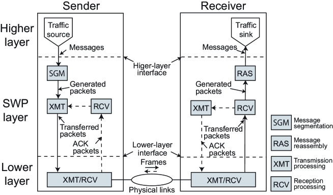
Figure 1: Communication network model.

In this section, we first explain the three-layered communication network model under consideration. Next, the model of data units introduced in this paper at the respective layer is described. In final, we explain some assumptions for analytical tractability.

II-A Layer model

To characterize the nature of RPSP and message segmentation, we consider a communication network of which conceptual representation is shown in Fig. 1. Each station (a sender and a receiver) has three layers. The middle layer is referred to as an SWP layer. It implements message segmentation-reassembly and error-recovery functions. The error-recovery function is assumed to be implemented in a stop-and-wait scheme. The layer above the SWP layer, namely the higher layer, contains a traffic source and sink. The traffic source generates the data units. On the other hand, the traffic sink terminates the corresponding data units. The layer below the SWP layer, namely the lower layer, contains an entity that can transfer data units over physical links at a sender.

II-B Data-unit model

We define data units exchanged between peer entities at the respective layer as follows:

Message: a data unit generated by a traffic source with a given size distribution of which function is denoted by $F^{(m)}(\cdot)$.

Packet: a data unit created from a message through segmentation function by adding a header and/or trailer, i.e., control information, to the (divided) message. We assume that size of SWP-layer’s control information is constant and equal to $\ell_{h}^{({\rm R})}$. Whenever a packet is created, a seqNum ($\geq 1$) is assigned. To model the RPSP explicitly, the packets are categorized into the following two kinds:

Generated packet: a packet that is generated from a message by a sender’s SWP layer at the original transmission. The message segmentation function implemented in the sender’s SWP layer enables a single message to be divided into several generated packets if the message size is larger than the payload size $\ell_{d}(>0)$. The receiver’s SWP layer performs a message reassembly function, thus reassembling the segmented generated packets before delivering them to the higher layer.

Transferred packet: a packet that is encapsulated into the frame. Due to RPSP, all the sizes of transferred packets with the same seqNum are equal to that of the generated packet.

Frame: a data unit that is made by encapsulating a transferred packet into a frame and by adding control information to the transferred packet, and will be transferred over physical links. The size of lower-layer’s control information is assumed to be cosntant and equal to $\ell_{h}^{({\rm L})}$.

II-C Assumptions

For analytical tractability, we make the following assumptions.

A1:

Message sizes are mutually independent and identically distributed according to a common message-size distribution function $F^{(m)}(\cdot)$. The distribution $F^{(m)}(\cdot)$ has a finite mean value $\ell^{(m)}$, which is referred to as the mean message size.

A2:

Frames are independently lost with probability

$$g(x),\ 0\leq g(x)<1,$$

where $x$ is the size of information field in the frame, equivalently, the size of a transferred packet.

A3:

The sender operates under a heavy traffic assumption, meaning that the sender’s SWP layer always has a generated packet available to be sent.

Example 1

Case of independent bit error prone links. Typical situations satisfying assumption A2 include the cases where frames are lost due to bit errors that occur independently. Letting $p_{e}$ be bi-error rate, $g(x)$ is given by

$$g(x) =1-(1-p_{e})^{x+\ell_{h}^{({\rm L})}},$$ (1)

where $x$ is the size of transferred packets.

III Analysis of size distributions for generated packets, transferred packets and frames

In this section, we derive the forms of a size distributions of generated packets, transferred packets and frames under assumptions mentioned in the preceding section.

III-A Form of generated packet size distribution

Let random variable $L^{(p)}$ be a size of generated packets. Denoting $F^{(p)}(\cdot)$ be a generated packet size distribution, that is $F^{(p)}(x)\stackrel{{\scriptstyle\triangle}}{{=}}\Pr.({L^{(p)}\leq x})$, from the argument [10], we have

$$F^{(p)}(x) =\left(1-\pi^{(\textrm{E})}\right)\textbf{1}(x-\ell_{d}-\ell_{h}^{({\rm R})})+\pi^{(\textrm{E})}F^{(\textrm{E})}(x),$$ (2)

where $\pi^{(\textrm{E})}$ is an occurrence probability of edge packets and $F^{(\textrm{E})}(\cdot)$ is a distribution of edge-packet sizes. The edge packet is defined as the final segmented generated-packet, if a message is segmented. It is identical with the original message if not segmented.

The forms of $\pi^{(\textrm{E})}$ and $F^{(\textrm{E})}(\cdot)$ are given by

$$\pi^{(\textrm{E})} =\cfrac{1}{\displaystyle\sum_{s=0}^{\infty}\,\int_{s\ell_{d}}^{\infty}\,dF^{(m)}(x)}=\cfrac{1}{\displaystyle\sum_{s=0}^{\infty}\,\left(1-F^{(m)}(s\ell_{d})\right),}$$ (3)

and

$$F^{(\textrm{E})}(x) =\begin{cases}0,&0\leq x<\ell_{h}^{({\rm R})},\\ \displaystyle\sum_{s=0}^{\infty}\left\{F^{(m)}(x+s\,\ell_{d}-\ell_{h}^{({\rm R})})-F^{(m)}(s\,\ell_{d})\right\},&\ell_{h}^{({\rm R})}\leq x\leq\ell_{d}+\ell_{h}^{({\rm R})},\\ 1,&x>\ell_{d}+\ell_{h}^{({\rm R})}.\end{cases}$$ (4)

Example 2

Case of discrete message-size distribution. Consider the case where the message-size distribution function $F^{(m)}(\cdot)$ is given by

$$F^{(m)}(x) =\sum_{i=1}^{n_{d}}\omega^{(m)}_{i}\textbf{1}(x-\ell^{(m)}_{i}),$$ (5)

where $n_{d}\geq 1$, $w^{(m)}_{i}>0$, $\ell^{(m)}_{i}>0$ for $i=1,2,\cdots,n_{d}$, and $\sum_{i=1}^{n_{d}}w^{(m)}_{i}=1$.

The form of $\pi^{(\textrm{E})}$ is given by $\{\sum_{i=1}^{n_{d}}w^{(m)}_{i}k_{i}\}^{-1}$ with $k_{i}=\lceil\ell^{(m)}_{i}/\ell_{d}\rceil$. This can be intuitively shown from the fact that 1) $k_{i}$ generated packets are created from one message of size $\ell^{(m)}_{i}$, and 2) they consist of $k_{i}-1$ generated packets of size $\ell_{d}$ (called body packets [10]) and one edge packet. The generated-packet-size distribution can be written as

$$F^{(p)}(x) =\left(1-\pi^{(\textrm{E})}\right)\,\textbf{1}(x-\ell_{d}-\ell_{h}^{({\rm R})})+\pi^{(\textrm{E})}\,\sum_{i=1}^{n_{d}}\,w^{(m)}_{i}\,\textbf{1}(x-\ell^{(m)}_{i}+(k_{i}-1)\,\ell_{d}-\ell_{h}^{({\rm R})}).$$ (6)

The form of (6) can be rewritten as

$$F^{(p)}(x) \stackrel{{\scriptstyle\triangle}}{{=}}\sum_{i=0}^{n_{d}}w^{(p)}_{i}\textbf{1}(x-\ell^{(p)}_{i}),$$ (7)

where

$$\begin{cases}w^{(p)}_{0}=1-\pi^{(\textrm{E})},\\ l^{(p)}_{0}=\ell_{d}+\ell_{h}^{({\rm R})},\end{cases}$$ (8)

$$\begin{cases}w^{(p)}_{i}=\pi^{(\textrm{E})}\,w^{(m)}_{i},\\ l^{(p)}_{i}=\ell^{(m)}_{i}-(k_{i}-1)\,\ell_{d}+\ell_{h}^{({\rm R})},\end{cases}i=1,2,\cdots,n_{d}.$$ (9)

 

Letting $\ell^{(p)}$ be the mean packet size, we have

$$\ell^{(p)} \stackrel{{\scriptstyle\triangle}}{{=}}\int_{0}^{\infty}\,x\,dF^{(p)}(x)=\pi^{(\textrm{E})}\,\ell^{(m)}+\ell_{h}^{({\rm R})}.$$ (10)

III-B Form of transferred packet size distribution

Let $F^{(q)}(\cdot)$ be a transferred packet size distribution. Denoting the number of retransmissions of the transferred packet with the same seqNum of the generated packet which size is equal to $L^{(p)}$ by $R$, we can prove the following proposition.

Proposition 1

The transferred packet size distribution $F^{(q)}(\cdot)$ is given by

$$F^{(q)}(y) =\begin{cases}0,&0\leq y<\ell_{h}^{({\rm R})},\\ \cfrac{\displaystyle\int_{x=\ell_{h}^{({\rm R})}}^{x=y}E\left[R+1\,|\,L^{(p)}=x\right]\,dF^{(p)}(x)}{E\left[R+1\right]},&\ell_{h}^{({\rm R})}\leq y\leq\ell_{d}+\ell_{h}^{({\rm R})},\\ 1,&y>\ell_{d}+\ell_{h}^{({\rm R})}.\end{cases}$$ (11)

Proof.

See Appendix A. ∎

From assumption A2, the form of $E[R+1\,|\,L^{(p)}=x]$ for $\ell_{h}^{({\rm R})}\leq x\leq\ell_{d}+\ell_{h}^{({\rm R})}$ is given by

$$E\left[R+1\,|\,L^{(p)}=x\right] =\left(1-g(x)\right)\,\sum_{r=0}^{n_{\textrm{RL}}}\,(r+1)\,\left\{g(x)\right\}^{r}+\left\{g(x)\right\}^{n_{\textrm{RL}}+1}\,\left(n_{\textrm{RL}}+1\right)$$

$$=\cfrac{1-\{g(x)\}^{n_{\textrm{RL}}+1}}{1-g(x)}\stackrel{{\scriptstyle\triangle}}{{=}}h(x,n_{\textrm{RL}}).$$ (12)

where $n_{\rm RL}(\geq 0)$ is the maximum number of retransmission attempts of the transferred packet with the same seqNum, referred to as retry limit.

Remark 1

Substitution of (2) into (11) yields $F^{(q)}(y)$ for $\ell_{h}^{({\rm R})}\leq y\leq\ell_{d}+\ell_{h}^{({\rm R})}$ given by

$$F^{(q)}(y) =\cfrac{\left(1-\pi^{(\textrm{E})}\right)\,h(\ell_{d}+\ell_{h}^{({\rm R})},n_{\textrm{RL}})\,\textbf{1}(x-\ell_{d}-\ell_{h}^{({\rm R})})+\pi^{(\textrm{E})}\,\displaystyle\int_{x=\ell_{h}^{({\rm R})}}^{x=y}\,h(x,n_{\textrm{RL}})\,dF^{(\textrm{E})}(x)}{E\left[R+1\right]},$$ (13)

where $E[R+1]$ is given by

$$E\left[R+1\right] =\left(1-\pi^{(\textrm{E})}\right)\,h(\ell_{d}+\ell_{h}^{({\rm R})},n_{\textrm{RL}})+\pi^{(\textrm{E})}\,\int_{\ell_{h}^{({\rm R})}}^{\ell_{d}+\ell_{h}^{({\rm R})}}\,h(x,n_{\textrm{RL}})\,dF^{(\textrm{E})}(x).$$ (14)

 

Example 3

RPSP effect when no frame is lost. Consider the case where no frame is lost. In this case, the number of retransmissions is equal to zero, i.e., $R=0$. From (11), $F^{(q)}(x)$ is identified with $F^{(p)}(x)$, implying that no effect of RPSP appears.   

Example 4

RPSP effect when generated packets are constant in size. Let us consider the case where generated packets have a common size $\ell_{c}(=\ell^{(p)})$, that is

$$F^{(p)}(x) =\textbf{1}(x-\ell_{c}).$$ (15)

Thypical situations include when message sizes follow the discrete distribution function given by (5) with $n_{d}=1$ and $\ell^{(m)}_{1}(=\ell_{c}-\ell_{h}^{({\rm R})})\leq\ell_{d}$, resulting in $\pi^{(\textrm{E})}=0$. Note that $F^{(p)}(x)$ can be approximated by $\textbf{1}(x-\ell_{d})$ if $\ell^{(m)}$ is large enough compared with $\ell_{d}$ from [10, Remark 3].

With (11) and (15), $F^{(q)}(x)$ is identified with $F^{(p)}(x)=\textbf{1}(x-\ell_{c})$, which indicates that no effect of RPSP appears.   

III-C Form of frame size distribution

Denote the frame size distribution by $F^{(f)}(\cdot)$. Since a frame contains a transferred packet and the size of control information added the transferred packet is $\ell_{h}^{({\rm L})}$, $F^{(f)}(x)$ is simply given by $F^{(q)}(x-\ell_{h}^{({\rm L})})$.

IV Goodput Analysis

In this section, first, we derive the form of goodput in a simple scenario. Next, we apply the result to an IEEE 802.11 DCF wireless network.

IV-A Form of goodput

Let $G$ be goodput of a single SWP connection, which is defined as the mean number of bits by a receiver’s higher layer entity across the higher layer interface per unit time. We denote the interdeparture time of the transferred packet by $T^{(cycle)}$. In addition, we denote the event meaning that the transferred packet is successfully transmitted by “delivery”. Then we can prove the following proposition.

Proposition 2

The form of goodput $G$ is given by

$$G =\cfrac{\displaystyle\int_{x=\ell_{h}^{({\rm R})}}^{\ell_{d}+\ell_{h}^{({\rm R})}}\,\Pr.(\text{\it delivery}\,|\,L^{(p)}=x)\,(x-\ell_{h}^{({\rm R})})\,dF^{(p)}(x)}{\displaystyle\int_{x=\ell_{h}^{({\rm R})}}^{\ell_{d}+\ell_{h}^{({\rm R})}}\,E\left[R+1\,|\,L^{(p)}=x\right]\,E\left[T^{(cycle)}\,|\,L^{(p)}=x\right]\,dF^{(p)}(x)}.$$ (16)

Proof.

See Appendix B. ∎

Note that assumption A2 yields the form of $\Pr.(\text{\it delivery}\,|\,L^{(p)}=x)$ given by

$$\Pr.(\text{\it delivery}\,|\,L^{(p)}=x) =1-\{g(x)\}^{n_{\textrm{RL}}+1}.$$ (17)

IV-B Application of goodput analysis to IEEE 802.11 DCF

We consider a simple scenario where just one sender and one receiver exist in a wireless network equipped with IEEE 802.11 DCF, which is an SWP protocol. Since no collision occurs, from the argument described in [6], the form of $E[T^{(cycle)}\,|\,L^{(p)}=x]$ in (16) can be simply written as

$$E\left[T^{(cycle)}\,|\,L^{(p)}=x\right] =\cfrac{(1-g(x))\,\sigma}{1-\left\{g(x)\right\}^{n_{\text{RL}}+1}}\displaystyle\sum_{r=0}^{n_{\text{RL}}}b_{r}\,\left\{g(x)\right\}^{r}$$

$$\quad+\left(1-g(x)\right)\,t_{\textrm{suc}}(x)+g(x)\,t_{\textrm{bit}}(x),$$ (18)

where

$\sigma$:

DCF backoff slot size

$b_{r}$:

mean value of the backoff counter of the $r$th backoff stage, i.e., the $r$th retransmission attempt of the transferred packet

$t_{\textrm{suc}}(x)$ and $t_{\textrm{bit}}(x)$:

mean interdeparture times of the transferred packet of size of $x$ when a transmission is successful and fails due to bit errors, respectively.

The value of $E[b_{r}]$ is equal to $\textrm{CW}_{r}/2$ because the backoff time at each transmission is uniformly chosen in the range $[0,\textrm{CW}_{r}]$ where $\textrm{CW}_{r}$ is $\min\{2^{r}\,(\textrm{CW}_{\min}+1)-1,\textrm{CW}_{\max}\}$ for $r=1,2,\cdots,n_{\textrm{RL}}$ and $\textrm{CW}_{0}$ is $\textrm{CW}_{\min}$. Assuming that propagation delay is negligible, we have

$$t_{\textrm{suc}}(x) =\cfrac{x+\ell_{\rm ACK}}{\mu_{d}}+\cfrac{2\,\ell_{h}^{({\rm L})}}{\mu_{b}}+t_{\rm SIFS}+t_{\rm DIFS},$$ (19)

$$t_{\textrm{bit}}(x) =\cfrac{x}{\mu_{d}}+\cfrac{\ell_{h}^{({\rm L})}}{\mu_{b}}+t_{\rm EIFS},$$ (20)

where $\mu_{d}$ is data-transmission rate, $\mu_{b}$ is basic-link rate, and $\ell_{\rm ACK}$ is ACK-packet size. Here, $t_{\rm SIFS}$, $t_{\rm DIFS}$ and $t_{\rm EIFS}$ are Short Inter Frame Space (IFS), DCF IFS and Extended IFS, respectively. The derivation of (IV-B) can be found in Appendix C.

V Numerical results and discussions

In this section, we examine the effect of RPSP on frame-size distributions and goodput by utilizing the results in Sections III and IV. We consider a scenario in which Web objects are transferred over the IEEE 802.11 DCF network where bit errors occur independently. In the following, we used the parameter values listed in Table I.

TABLE I: Parameter values used to obtain numerical results

Parameter	Value
Basic-link rate $\mu_{b}$	$1$ Mbps
Data-transmission rate $\mu_{d}$	$11$ Mbps
SWP layer information field size $\ell_{h}^{({\textrm{R}})}$	$34$ bytes
Lower layer information field size $\ell_{h}^{({\textrm{L}})}$	$24$ bytes
Slot time $\sigma$	$20~{}\mu$sec
Short IFS $t_{\rm SIFS}$	$10~{}\mu$sec
DCF IFS $t_{\rm DIFS}$	$50~{}\mu$sec
Extended IFS $t_{\rm EIFS}$	$263~{}\mu$sec
ACK-packet size $\ell_{\rm ACK}$	$14$ bytes
Minimum contention window size $\textrm{CW}_{\min}$	$31$
Maximum contention window size $\textrm{CW}_{\max}$	$1023$

Two kinds of Web pages are considered: static and dynamic Web pages. We shall use the following Web object size distributions from traffic measurements [8, 11].

• Static Web objects: The sizes of the static Web objects is assumed to follow a lognormal distribution given by

  $$F^{(m)}(x) =\begin{cases}\displaystyle\int_{y=0}^{y=x}\cfrac{1}{\sqrt{2\pi}\sigma y}e^{\tfrac{-\left(\log y-\mu\right)^{2}}{2\sigma^{2}}}dy,&x>0,\\ 0,&x\leq 0.\end{cases}$$ (21)

  The distribution parameters $\mu$ and $\sigma$ are assumed to be $6.34$ and $2.07$, respectively, on the basis of the measured mean message size $\ell^{(m)}=4827$ bytes and the measured standard deviation $\sigma^{(m)}=41,008$ bytes. Note that this lognormal distribution can represent a long-tailed property.

• Dynamic Web objects: The sizes of the dynamic Web objects are assumed to follow a Weibull distribution:

  $$F^{(m)}(x) =\begin{cases}1-e^{-(\lambda\,x)^{\nu}},&x>0,\\ 0,&\text{$x\leq 0$}.\end{cases}$$ (22)

  The scale parameter $\lambda$ and the shape parameter $\nu$ are assumed to be $4.02\times 10^{-4}$ and $1.9$, respectively, which fit the measured dynamic Web object size distribution for one case of an entertainment site [11]. Note that the Weibull distribution in this case is not a long-tailed distribution because the shape parameter $\nu$ is not smaller than $1$. The mean message size $\ell^{(m)}$ is $2207.37$ bytes, and the standard deviation $\sigma^{(m)}$ is $1208.43$ bytes.

V-A Effect of RPSP on frame size distribution

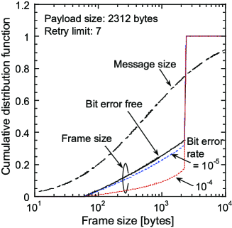
a) Case of static Web objects.

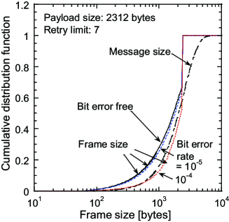
b) Case of dynamic Web objects.

Figure 2: Cumulative frame size distributions $F^{(f)}(\cdot)$ for different bit error rates $p_{e}$.

Figures 2 (a) and (b) show the distributions of frame sizes $F^{(f)}(\cdot)$ for different bit error rates $p_{e}$ of static and dynamic Web objects, respectively. We used payload size $\ell_{d}$ of $2312$ bytes and retry limit $n_{\textrm{RL}}$ of $7$. Note that $2312$ bytes of the payload size $\ell_{d}$ is the maximum transmission unit size of IEEE 802.11 wireless LANs and $7$ of retry limit $n_{\textrm{RL}}$ is the default value [1].

These figures show that the frame size distribution $F^{(f)}(\cdot)$ for high bit error rates is significantly different from that for bit error free. Thus, we can see that the effect of RPSP produces a more concave curve for the transferred packet size distribution when the bit error rate is higher.

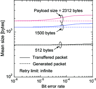
a) Case of static Web objects.

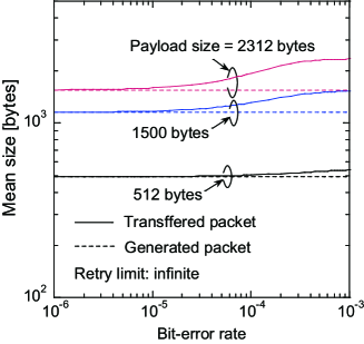
b) Case of dynamic Web objects.

Figure 3: Mean transferred packet size $\ell^{(q)}$ and mean generated packet size $\ell^{(p)}$ versus bit error rates $p_{e}$ when retry limit $n_{\textrm{RL}}$ goes to infinite for different payload sizes $\ell_{d}$.

TABLE II: Mean size of transferred packets $\ell^{(q)}$ for different bit error rates $p_{e}$ when payload size $\ell_{d}$ is 2312 byte and retry limit $n_{\textrm{RL}}$ goes to infinite.

$p_{e}$	$10^{-6}$	$10^{-5}$	$10^{-4}$	$10^{-3}$
Static Web objects	$1761.4$	$1815.0$	$2161.4$	$2344.6$
Dynamic Web objects	$1552.0$	$1592.9$	$1926.8$	$2334.8$

Note: Mean sizes of transferred packets $\ell^{(q)}$ are represented in units of bytes. Maximum size of generated packets $\ell^{(p)}_{\max}$ of static and dynamic Web objects is $2346.0$ bytes, which is $\ell_{d}+\ell_{h}^{({\rm R})}$.

Let $\ell^{(q)}$ be the mean transferred packet size, that is $\ell^{(q)}\stackrel{{\scriptstyle\triangle}}{{=}}\int_{0}^{\infty}\,x\,dF^{(q)}(x)$. To investigate the effect of RPSP when retry limit $n_{\textrm{RL}}$ goes to infinite, Figs. 3 (a) and (b) show mean transferred packet size $\ell^{(q)}$ and mean generated packet size $\ell^{(p)}$ of static and dynamic Web objects, respectively, versus bit error rates $p_{e}$ for different payload sizes $\ell_{d}$. Table II lists mean size of transferred packets $\ell^{(q)}$ for different bit error rates $p_{e}$ when payload size $\ell_{d}$ is 2312 byte and retry limit $n_{\textrm{RL}}$ goes to infinite. in the cases of static and dynamic Web objects. From Figs. 3 (a) and (b), and Table II, we find that the RPSP effect appears when the bit error rate $p_{e}$ exceeds $10^{-5}$. The reason for this is that longer transferred packets are likely to be retransmitted more times. Letting random variables $L^{(p)}_{\kappa}$ and $R_{\kappa}$ be size and the number of retransmissions of the transferred packet of which seqNum is $\kappa$, respectively, this implies that $h(x^{(p)}_{\kappa},\infty)=E[R_{\kappa}+1\,|\,L^{(p)}_{\kappa}=x^{(p)}_{\kappa}]>h(x^{(p)}_{\kappa^{\prime}},\infty)$ if $x^{(p)}_{\kappa}>x^{(p)}_{\kappa^{\prime}}$.

Let $\ell^{(p)}_{\max}$ be the maximum generated packet size, i.e., $\ell^{(p)}_{\max}=\min\{l;F^{(p)}(l)=1\}$. From an inspection of Figs. 3 (a) and (b), and Table II, we find that $\ell^{(q)}$ reaches around $\ell^{(p)}_{\max}$ as $p_{e}\to 1$. This implies that the number of transmissions of the longest transferred packets is dominant in the total number of transmissions of all transferred packets due to RPSP. Then, we have the following conjecture.

Conjecture 1

Asymptotic bound on mean transferred packet size. We denote the asymptotic bound on the mean transferred packet size by $\ell^{(q)}_{\max}$. That is the finite limit of the mean transferred packet size as the value of $p_{e}$ approaches one. Then, we have

$$\ell^{(q)}\to\ell^{(q)}_{\max} =\ell^{(p)}_{\max},\qquad\text{as $p_{e}\to 1$.}$$ (23)

 

Appendix D provides the proof of conjecture 1 in the case of a discrete generated packet size distribution.

From conjecture 1, we find that RPSP effect appears stronger when $\ell^{(p)}_{\max}/\ell^{(p)}$ increases. If the mean message size $\ell^{(m)}$ is enough large compared with payload size $\ell_{d}$, resulting in $\ell^{(p)}\approx\ell_{d}=\ell^{(p)}_{\max}$, RPSP effect is likely to disappear.

V-B Effect of RPSP on goodput

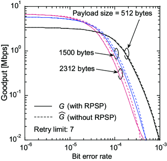
a) Case of static Web objects.

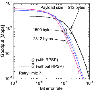
b) Case of dynamic Web objects.

Figure 4: Goodput $G$ and $\hat{G}$ versus bit error rate $p_{e}$ for different payload sizes $\ell_{d}$ when limit retry $n_{\textrm{RL}}$ is $7$.

In this subsection, we investigate the RPSP effect on goodput. To do this, we introduce $\hat{G}$ which is obtained from the approximation of $F^{(q)}(x)=\textbf{1}(x-\ell^{(p)})$. Thus,

$$\hat{G} =\cfrac{\Pr.(\text{\it delivery}\,|\,L^{(p)}=\ell^{(p)})\,(\ell^{(p)}-\ell_{h}^{({\rm R})})}{E\left[R+1\,|\,L^{(p)}=\ell^{(p)}\right]\,E\left[T^{(cycle)}\,|\,L^{(p)}=\ell^{(p)}\right]}.$$ (24)

Cleary, the value of $\hat{G}$ is equal to that of $\hat{G}$ when no transferred packet loss happens because RPSP effect disappears (see Example 3).

Figures 4 (a) and (b) show $G$ and $\hat{G}$ versus bit error rate $p_{e}$ for different payload sizes $\ell_{d}$ when limit retry $n_{\textrm{RL}}$ is $7$ in the cases of static and dynamic Web objects, respectively. From these figures, we find that RPSP leads to overestimate goodput obtained from the traditional model which assume that the transferred packets is constant in size. As similar to the results mentioned in the preceding subsection, we find that the RPSP effect on goodput appears when the bit error rate $p_{e}$ exceeds $10^{-5}$ and payload size $\ell_{d}$ exceeds $1500$ bytes.

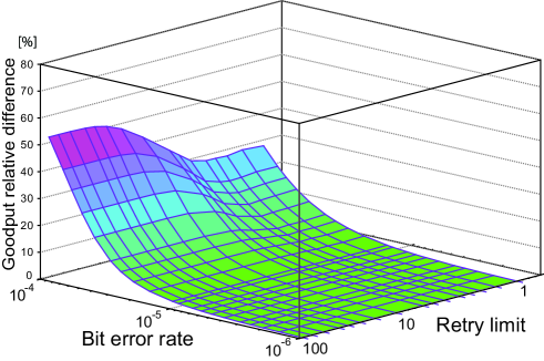
Figure 5: Goodput relative difference $(\hat{G}-G)/G$ versus bit error rate $p_{e}$ and retry limit $n_{\textrm{RL}}$ when payload size $\ell_{d}$ is 2312 bytes in the case of static Web objects.

Figure 5 shows goodput relative difference $(\hat{G}-G)/G$ versus bit error rate $p_{e}$ and retry limit $n_{\textrm{RL}}$ when payload size $\ell_{d}$ is 2312 bytes in the case of static Web objects. From this figure, we find that the effect of RPSP on goodput appears stronger when bit error rate $p_{e}$ increases for large enough retry limits.

VI Conclusion

In this paper, we have described a data-unit-size distribution model to represent the retransmitted packet size (RPSP) property and message segmentation behavior when frames are independently lost and they are recovered by a stop-and-wait protocol. RPSP means that all transferred packets at retransmissions with the same sequence number have the same size at the original transmission, which is identical to the packet generated from a message, namely, generated packets. Moreover, we have derived the goodput formula using an approach to derive the data-unit-size distribution. We have shown that the RPSP effect appears stronger when the maximum generated packet size is larger than the mean generated packet size. From numerical results, we have demonstrated that the RPSP effect on frame size distributions and goodput appears when the bit error rate exceeds $10^{-5}$ and payload size exceeds $1500$ bytes in a scenario where static Web objects are delivered over an IEEE 802.11 DCF wireless network.

The remaining issues include modeling a scenario where the collisions happen over a wireless network with bit errors occurring in burst.

Appendix A Proof of Proposition 1

First, without loss of generality, we consider the case of discrete message size distributions, resulting in the form of discrete generated packet size distributions given by (7). Substituting (7) into (11), we have

$$F^{(q)}(x)=\sum_{i=0}^{n_{d}}w^{(q)}_{i}\textbf{1}(x-\ell^{(p)}_{i}),$$ (25)

where $w^{(q)}_{i}$ for $i=0,1,\cdots,n_{d}$ is given by

$$w^{(q)}_{i} =\cfrac{w^{(p)}_{i}\,E\left[R+1\,|\,L^{(p)}=\ell^{(p)}_{i}\right]}{E\left[R+1\right]}$$

$$=\cfrac{w^{(p)}_{i}\,E\left[R+1\,|\,L^{(p)}=\ell^{(p)}_{i}\right]}{\displaystyle\sum_{j=0}^{n_{d}}\,w^{(p)}_{j}\,E\left[R+1\,|\,L^{(p)}=\ell^{(p)}_{j}\right]}.$$ (26)

To derive (25) and (A), we introduce the following notations of the generated packet of size equal to $\ell^{(p)}_{i}$ for $i=0,1,\cdots,n_{d}$:

$M_{i}(t)$:

number of attempts of transmissions of transferred packets prior to time $t$,

$Q_{i,\kappa}(t)$:

number of attempts of transmissions of transferred packets that are created from the generated packet with seqNum of $\kappa$ prior to time $t$.

A sender transmits the transferred packet of which seqNum is $\kappa$ and size is $\ell^{(p)}_{i}$ $Q_{i,\kappa}(t)$ times prior to time $t$. From the argument of a probability mass function, the form of $w^{(q)}_{i}$ can be written as

$$w^{(q)}_{i}=\lim_{t\to\infty}\cfrac{\displaystyle\sum_{\kappa=1}^{M_{i}(t)}\,Q_{i,\kappa}(t)}{\displaystyle\sum_{i=0}^{n_{d}}\sum_{\kappa=1}^{M_{i}(t)}\,Q_{i,\kappa}(t)}=\left(\lim_{t\to\infty}\cfrac{\displaystyle\sum_{j=0}^{n_{d}}M_{j}(t)}{\displaystyle\sum_{i=0}^{n_{d}}\sum_{\kappa=1}^{M_{i}(t)}\,Q_{i,\kappa}(t)}\right)\left(\lim_{t\to\infty}\cfrac{M_{i}(t)}{\displaystyle\sum_{j=0}^{n_{d}}M_{j}(t)}\right)\left(\lim_{t\to\infty}\cfrac{\displaystyle\sum_{\kappa=1}^{M_{i}(t)}\,Q_{i,\kappa}(t)}{M_{i}(t)}\right).$$ (27)

The form of $w^{(p)}_{i}$ in (A) is given by

$$w^{(p)}_{i} =\Pr.(\text{the generated packet of size is equal to $\ell^{(p)}_{i}$})=\lim_{t\to\infty}\cfrac{M_{i}(t)}{\displaystyle\sum_{j=0}^{n_{d}}M_{j}(t)}.$$ (28)

Let $R_{\kappa}$ be the number of retransmissions of the generated packet of which seqNum is $\kappa$. Under assumption A2, $\{R_{\kappa}\}$ forms a sequence of mutually independent and identically distributed random variables with finite value of $E[R_{\kappa}](\stackrel{{\scriptstyle\triangle}}{{=}}E[R])$. From the Law of Large Numbers, we have

$$E[R+1] =\lim_{t\to\infty}\cfrac{\displaystyle\sum_{i=0}^{n_{d}}\sum_{\kappa=1}^{M_{i}(t)}\,Q_{i,\kappa}(t)}{\displaystyle\sum_{j=0}^{n_{d}}M_{j}(t)},$$ (29)

and

$$E[R+1\,|\,L^{(p)}=\ell^{(p)}_{i}] =\lim_{t\to\infty}\cfrac{\displaystyle\sum_{\kappa=1}^{M_{i}(t)}\,Q_{i,\kappa}(t)}{M_{i}(t)}.$$ (30)

Substituting (28), (29) and (30) into (27), we obtain (25) and (A).

Next, we provide an alternative derivation of (11). Consider a packet size sequence $\{L^{(q)}_{n};n\in\mathcal{N}(\stackrel{{\scriptstyle\triangle}}{{=}}\{1,2,\cdots\})\}$ where $L^{(q)}_{n}$ means the transferred packet size of the $n$th transmission. Forming transferred packets with the same seqNum a group, we constitute a sequence $\{L^{(q)}_{n}\}$ expressed as

$$\{L^{(q)}_{n};n\in\mathcal{N}\}=\\ \Big{\{}\overbrace{L^{(p)}_{1},\cdots,L^{(p)}_{1},L^{(p)}_{1}}^{R_{1}+1},\,\overbrace{L^{(p)}_{2},\cdots,L^{(p)}_{2},L^{(p)}_{2}}^{R_{2}+1},\cdots,\overbrace{L^{(p)}_{\kappa},\cdots,L^{(p)}_{\kappa},L^{(p)}_{\kappa}}^{R_{\kappa}+1},\cdots\Big{\}}.$$ (31)

As shown in (31), the random variable $L^{(p)}_{\kappa}$ appears $R_{\kappa}+1$ times consecutively in the sequence of the transferred packets with seqNum of $\kappa$. Therefore, we obtain (11).

Appendix B Proof of Proposition 2

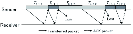
Figure 6: The example of $\{T_{i,j,\kappa}\}$ under a heavy traffic condition in the case of $n_{d}$ equal to one.

Similar to the proof mentioned in Appendix A, we consider the case of discrete message size distributions given by (7). Substituting (7) into (16), we have

$$G =\cfrac{\displaystyle\sum_{i=0}^{n_{d}}\,w^{(p)}_{i}\,\Pr.(\text{\it delivery}\,|\,L^{(p)}=\ell^{(p)}_{i})\,\left(\ell^{(p)}_{i}-\ell_{h}^{({\rm R})}\right)}{\displaystyle\sum_{i=0}^{n_{d}}\,w^{(p)}_{i}\,E\left[R+1\,|\,L^{(p)}=\ell^{(p)}_{i}\right]\,E\left[T^{(cycle)}\,|\,L^{(p)}=\ell^{(p)}_{i}\right]}.$$ (32)

To derive (32), we introduce the following additional notations for the generated packet of size equal to $\ell^{(p)}_{i}$ for $i=0,1,\cdots,n_{d}$:

$N_{i}(t)$:

number of successful transmissions of transferred packets prior to time $t$,

$T_{i,j,\kappa}$:

transmission of the $j(\leq Q_{i,\kappa}(t))$th attempt for the transferred packet of which seqNum is $\kappa(\leq M_{i}(t))$. The example of $\{T_{i,j,\kappa}\}$ under a heavy traffic condition in the case of $n_{d}$ equal to one is shown in Fig. 6.

For large enough $t$, we have

$$t \approx\sum_{i=0}^{n_{d}}\,\sum_{\kappa=1}^{M_{i}(t)}\,\sum_{j=1}^{Q_{i,\kappa}(t)}\,T_{i,j,\kappa}.$$ (33)

The definition of goodput yields

$$G =\lim_{t\to\infty}\cfrac{\displaystyle\sum_{i=0}^{n_{d}}N_{i}(t)\,\left(\ell^{(p)}_{i}-\ell_{h}^{({\rm R})}\right)}{t}.$$ (34)

Substituting (33) into (34), we have

$$G =\lim_{t\to\infty}\cfrac{\displaystyle\sum_{i=0}^{n_{d}}N_{i}(t)\,\left(\ell^{(p)}_{i}-\ell_{h}^{({\rm R})}\right)}{\displaystyle\sum_{i=0}^{n_{d}}\,\sum_{j=1}^{Q_{i,\kappa}(t)}\,\sum_{\kappa=1}^{M_{\kappa}(t)}\,T_{i,j,\kappa}}=\left(\lim_{t\to\infty}\cfrac{\displaystyle\sum_{i=0}^{n_{d}}N_{i}(t)\,\left(\ell^{(p)}_{i}-\ell_{h}^{({\rm R})}\right)}{\displaystyle\sum_{i=0}^{n_{d}}\,\sum_{\kappa=1}^{M_{i}(t)}\,Q_{i,\kappa}(t)}\right)\left(\lim_{t\to\infty}\cfrac{\displaystyle\sum_{i=0}^{n_{d}}\sum_{\kappa=1}^{M_{\kappa}(t)}\,Q_{i,\kappa}(t)}{\displaystyle\sum_{i=0}^{n_{d}}\,\sum_{j=1}^{Q_{i,\kappa}(t)}\,\sum_{\kappa=1}^{M_{i}(t)}\,T_{i,j,\kappa}}\right).$$ (35)

The form of $\Pr.(\text{\it delivery}\,|\,L^{(p)}=\ell^{(p)}_{i})$ is given by

$$\Pr.(\text{\it delivery}\,|\,L^{(p)}=\ell^{(p)}_{i}) =\lim_{t\to\infty}\cfrac{N_{i}(t)}{M_{i}(t)}.$$ (36)

From (28), (29) and (36), we have

$$\lim_{t\to\infty}\cfrac{N_{i}(t)}{\displaystyle\sum_{i=0}^{n_{d}}\,\sum_{\kappa=1}^{M_{i}(t)}\,Q_{i,\kappa}(t)} =\left(\lim_{t\to\infty}\cfrac{\displaystyle\sum_{j=0}^{n_{d}}\,M_{j}(t)}{\displaystyle\sum_{i=0}^{n_{d}}\,\sum_{\kappa=1}^{M_{i}(t)}\,Q_{i,\kappa}(t)}\right)\left(\lim_{t\to\infty}\cfrac{M_{i}(t)}{\displaystyle\sum_{j=0}^{n_{d}}\,M_{j}(t)}\right)\left(\lim_{t\to\infty}\cfrac{N_{i}(t)}{M_{i}(t)}\right)$$

$$=\cfrac{1}{E[R+1]}\cdot w^{(p)}_{i}\cdot\Pr.(\text{\it delivery}\,|\,L^{(p)}=\ell^{(p)}_{i}).$$ (37)

The first term of (35) can be rewritten as

$$\lim_{t\to\infty}\cfrac{\displaystyle\sum_{i=0}^{n_{d}}N_{i}(t)\,\left(\ell^{(p)}_{i}-\ell_{h}^{({\rm R})}\right)}{\displaystyle\sum_{i=0}^{n_{d}}\sum_{\kappa=1}^{M_{i}(t)}\,Q_{i,\kappa}(t)} =\cfrac{\displaystyle\sum_{i=0}^{n_{d}}w^{(p)}_{i}\,\Pr.(\text{\it delivery}\,|\,L^{(p)}=\ell^{(p)}_{i})\,\left(\ell^{(p)}_{i}-\ell_{h}^{({\rm R})}\right)}{E[R+1]}.$$ (38)

Under the assumption of A2, $\{T_{i,1,1},T_{i,1,2},\cdots,T_{i,2,1},T_{i,2,2},\cdots\}$ forms a sequence of mutually independent and identically distibuted random variables with a common distribution with mean $E[T^{(cycle)}\,|\,L^{(p)}=\ell^{(p)}_{i}]$. From the Law of the Large Numbers, we have

$$\lim_{t\to\infty}\cfrac{\displaystyle\sum_{\kappa=1}^{M_{i}(t)}\,\sum_{j=1}^{Q_{i,\kappa}(t)}\,T_{i,j,\kappa}}{\displaystyle\sum_{\kappa=1}^{M_{i}(t)}\,Q_{i,\kappa}(t)} =E\left[T^{(cycle)}\,|\,L^{(p)}=\ell^{(p)}_{i}\right].$$ (39)

The inverse of the last term of (35) can be rewritten as

$$\lim_{t\to\infty}\cfrac{\displaystyle\sum_{i=0}^{n_{d}}\,\sum_{\kappa=1}^{M_{i}(t)}\,\sum_{j=1}^{Q_{i,\kappa}(t)}\,T_{i,j,\kappa}}{\displaystyle\sum_{i=0}^{n_{d}}\sum_{\kappa=1}^{M_{i}(t)}\,Q_{i,\kappa}(t)}\\ =\displaystyle\sum_{i=0}^{n_{d}}\left(\lim_{t\to\infty}\cfrac{\displaystyle\sum_{j=0}^{n_{d}}M_{j}(t)}{\displaystyle\sum_{i=0}^{n_{d}}\sum_{\kappa=1}^{M_{i}(t)}\,Q_{i,\kappa}(t)}\right)\left(\lim_{t\to\infty}\cfrac{M_{i}(t)}{\displaystyle\sum_{j=0}^{n_{d}}\,M_{j}(t)}\right)\left(\lim_{t\to\infty}\cfrac{\displaystyle\sum_{\kappa=1}^{M_{i}(t)}\,Q_{i,\kappa}(t)}{M_{i}(t)}\right)\left(\lim_{t\to\infty}\cfrac{\displaystyle\sum_{\kappa=1}^{M_{i}(t)}\,\sum_{j=1}^{Q_{i,\kappa}(t)}\,T_{i,j,\kappa}}{\displaystyle\sum_{\kappa=1}^{M_{i}(t)}\,Q_{i,\kappa}(t)}\right)$$ (40)

Substituting (28), (29), (30) and (39) into the above equation, we have

$$\lim_{t\to\infty}\cfrac{\displaystyle\sum_{i=0}^{n_{d}}\,\sum_{\kappa=1}^{M_{i}(t)}\,\sum_{j=1}^{Q_{i,\kappa}(t)}\,T_{i,j,\kappa}}{\displaystyle\sum_{i=0}^{n_{d}}\sum_{\kappa=1}^{M_{i}(t)}\,Q_{i,\kappa}(t)} =\cfrac{\displaystyle\sum_{i=0}^{n_{d}}w^{(p)}_{i}\,E\left[R+1\,|\,L^{(p)}=\ell^{(p)}_{i}\right]\,E\left[T^{(cycle)}\,|\,L^{(p)}=\ell^{(p)}_{i}\right]}{E[R+1]}.$$ (41)

Substitution of (38) and (41) into (35) yields (32).

Appendix C Derivation of (IV-B)

Because no collision occurs, from the argument of [6], we have

$$E\left[T^{(cycle)}\,|\,L^{(p)}=x\right] =\cfrac{\left(1-\tau(x)\right)\,\sigma}{\tau(x)}+\left(1-g(x)\right)\,t_{\textrm{suc}}(x)+g(x)\,t_{\textrm{bit}}(x),$$ (42)

where $\tau(x)$ is the probability that a sender can transmit a transferred packet of size equal to $x$. From the argument of [12], $\tau(x)$ is given by

$$\tau(x) =\cfrac{1}{1+\cfrac{1-g(x)}{1-\left\{g(x)\right\}^{n_{\text{RL}}+1}}\displaystyle\sum_{r=0}^{n_{\text{RL}}}b_{r}\,\left\{g(x)\right\}^{r}}.$$ (43)

Substitution (43) into (42), we obtain (IV-B).

Appendix D Proof of Conjecture 1

Suppose that the generated packets sizes follow the discrete distribution given by (7). By substitution of (7) into (11), the transferred packet size distribution $F^{(q)}(\cdot)$ is given by

$$F^{(q)}(x) \stackrel{{\scriptstyle\triangle}}{{=}}\sum_{i=0}^{n_{d}}w^{(q)}_{i}\textbf{1}(x-\ell^{(q)}_{i}),$$ (44)

where

$$w^{(q)}_{i} =\cfrac{w^{(p)}_{i}\,h(\ell^{(p)}_{i},n_{\textrm{RL}})}{\displaystyle\sum_{j=0}^{n_{d}}\,w^{(p)}_{j}\,h(\ell^{(p)}_{j},n_{\textrm{RL}})},\quad i=0,1,\cdots,n_{d},$$ (45)

because $E[R+1\,|\,L^{(p)}=\ell^{(p)}_{i}]=h(\ell^{(p)}_{i},n_{\textrm{RL}})$ and $E[R+1]=\sum_{j=0}^{n_{d}}\,w^{(p)}_{j}\,h(\ell^{(p)}_{j},n_{\textrm{RL}})$.

Let $i_{\max}$ be the index corresponding to the maximum generated packet size $\ell^{(p)}_{\max}$. Thus,

$$i_{\max}=\operatorname*{arg\,max}_{i\in\{0,1,\cdots,n_{d}\}}\{\ell^{(p)}_{i}\}.$$ (46)

We let $\bar{w}^{(q)}_{i}$ be a finite limit of the weight corresponding to discrete transferred packet size $\ell^{(p)}_{i}$ as $p_{e}\to 1$ and $n_{\textrm{RL}}\to\infty$ for $i=0,1,\cdots,n_{d}$. From $\lim_{n_{\textrm{RL}}\to\infty}h(x,n_{\textrm{RL}})=1/(1-g(x))=1/(1-p_{e})^{x+\ell_{h}^{({\textrm{L}})}}$ if $0\leq g(x)<1$, we have

$$\bar{w}^{(q)}_{i} =\lim_{p_{e}\to 1}\,\lim_{n_{\textrm{RL}}\to\infty}\cfrac{w^{(p)}_{i}\,h(\ell^{(p)}_{i},n_{\textrm{RL}})}{\displaystyle\sum_{j=0}^{n_{d}}\,w^{(p)}_{j}\,h(\ell^{(p)}_{j},n_{\textrm{RL}})}=\lim_{p_{e}\to 1}\,\cfrac{w^{(p)}_{i}}{(1-p_{e})^{\ell^{(p)}_{i}+\ell_{h}^{({\textrm{L}})}}}\cfrac{1}{\displaystyle\sum_{j=0}^{n_{d}}\cfrac{w^{(p)}_{j}}{(1-p_{e})^{\ell^{(p)}_{j}+\ell_{h}^{({\textrm{L}})}}}}$$

$$=\lim_{p_{e}\to 1}\,\cfrac{w^{(p)}_{i}}{(1-p_{e})^{\ell^{(p)}_{i}+\ell_{h}^{({\textrm{L}})}}}\cfrac{(1-p_{e})^{\ell^{(p)}_{\max}+\ell_{h}^{({\textrm{L}})}}}{\displaystyle\sum_{j=0}^{n_{d}}\cfrac{w^{(p)}_{j}}{(1-p_{e})^{\ell^{(p)}_{\max}-\ell^{(p)}_{j}}}}$$

$$=\lim_{p_{e}\to 1}\,\cfrac{w^{(p)}_{i}}{(1-p_{e})^{\ell^{(p)}_{i}+\ell_{h}^{({\textrm{L}})}}}\cfrac{(1-p_{e})^{\ell^{(p)}_{\max}+\ell_{h}^{({\textrm{L}})}}}{\displaystyle\sum_{{j=0,j\neq i_{\max}}}^{n_{d}}w^{(p)}_{j}(1-p_{e})^{\ell^{(p)}_{\max}-\ell^{(p)}_{j}}+w^{(p)}_{\max}}$$

$$=\begin{cases}1,&\text{for $i=i_{\max}$}\\ 0,&\text{for $i\neq i_{\max}$}\end{cases}.$$ (47)

Thus, we have

$$F^{(q)}(x)\to\textbf{1}(x-\ell^{(p)}_{\max}),\qquad\text{as $p_{e}\to 1$.}$$ (48)

Therefore, we obtain (23).

References

- [1] IEEE Standard for Information technology– Telecommunications and information exchange between systems – Local and metropolitan area networks – Specific requirements Part 11: Wireless LAN Medium Access Control (MAC) and Physical Layer (PHY) Specifications. IEEE Computer Society, June 2007.
- [2] T. Ikegawa and Y. Takahashi, “Analysis of mean frame size of Bernoulli wireless links with reliable-transmission window-based protocol,” in Proc. WiOpt’04: the 2nd International Symposium on Modeling and Optimization in Mobile, Ad Hoc, and Wireless Networks, Mar. 2004, pp. 402–403.
- [3] ——, “The effect of retransmitted packet size preservation property on TCP goodput over links with Bernoulli bit-errors,” in Proc. WiOpt’05: the 3rd International Symposium on Modeling and Optimization in Mobile, Ad Hoc, and Wireless Networks, Apr. 2005, pp. 21–28.
- [4] ——, “Effect of retransmitted packet size preservation property for wireless networks with a reliable communication protocol,” in Proc. ACM MSWiM’05: the 8th ACM International Symposium on Modeling, Analysis and Simulation of Wireless and Mobile Systems, Oct. 2005, pp. 313–317.
- [5] G. Bianchi, “Performance analysis of the IEEE 802.11 distributed coordination function,” IEEE Journal on Selected Areas in Communications, vol. 18, no. 3, pp. 535–547, Mar. 2000.
- [6] P. Chatzimisios, A. Boucouvalas, and V. Vitsas, “Influence of channel BER on IEEE 802.11 DCF,” Electronics Letters, vol. 39, no. 23, pp. 1687–1689, Nov. 2003.
- [7] H. Chen, “Revisit of the markov model of IEEE 802.11 DCF for an error-prone channel,” IEEE Communications Letters, vol. 15, no. 12, pp. 1278–1280, Dec. 2011.
- [8] M. Molina, P. Castelli, and G. Foddis, “Web traffic modeling exploiting TCP connections’ temporal clustering through HTML-REDUCE,” IEEE Network, vol. 14, no. 3, pp. 46–55, May/June 2000.
- [9] C. Na, J. Chen, and T. Rappaport, “Measured traffic statistics and throughput of IEEE 802.11b public WLAN hotspots with three different applications,” IEEE Transactions on Wireless Communications, vol. 5, no. 11, pp. 3296–3305, Nov. 2006.
- [10] T. Ikegawa, Y. Kishi, and Y. Takahashi, “Data-unit-size distribution model when message segmentations occur,” Performance Evaluation, vol. 69, no. 1, pp. 1–16, Jan. 2012.
- [11] W. Shi, E. Collins, and V. Karamcheti, “Modeling object characteristics of dynamic Web content,” Journal of Parallel and Distributed Computing, vol. 63, no. 10, pp. 963–980, Oct. 2003.
- [12] G. Bianchi and I. Tinnirello, “Remarks on IEEE 802.11 DCF performance analysis,” IEEE Commun. Lett., vol. 9, no. 8, pp. 765–767, Aug. 2005.