Thermal Inflation with a Thermal Waterfall Scalar Field Coupled to a Light Spectator Scalar Field
Arron Rumsey
September 2016
This thesis is submitted in partial fulfillment of the requirements for the degree of Master of Philosophy (MPhil) at Lancaster University. No part of this thesis has been previously submitted for the award of a higher degree.

Abstract

This thesis begins with an introduction to the state of the art of modern Cosmology. The field of Particle Cosmology is then introduced and explored, in particular with regard to the study of cosmological inflation. We then introduce a new model of Thermal Inflation, in which the mass of the thermal waterfall field responsible for the inflation is dependent on a light spectator scalar field. The model contains a variety of free parameters, two of which control the power of the coupling term and the non-renormalizable term. We use the $\delta N$ formalism to investigate the “end of inflation” and modulated decay scenarios in turn to see whether they are able to produce the dominant contribution to the primordial curvature perturbation $\zeta$. We constrain the model and then explore the parameter space. We explore key observational signatures, such as non-Gaussianity, the scalar spectral index and the running of the scalar spectral index. We find that for some regions of the parameter space, the ability of the model to produce the dominant contribution to $\zeta$ is excluded. However, for other regions of the parameter space, we find that the model yields a sharp prediction for a variety of parameters within the model.

Chapter 1 Introduction

Cosmological Inflation is a leading candidate for the solution of the three main problems of the standard Big Bang scenario: the Horizon, Flatness and Relic problems. It also has the ability to seed the initial conditions required to explain the observed large-scale structure of the Universe. (For a textbook on this topic, see [1].) In the simplest scenario, quantum fluctuations of a scalar field are converted to classical perturbations around the time of horizon exit, after which they become frozen. This gives rise to the primordial curvature perturbation, $\zeta$, which grows under the influence of gravity to give rise to all of the large-scale structure in the Universe. The observed value of the spectrum of the primordial curvature perturbation is $\mathcal{P}_{\zeta}^{\frac{1}{2}}(k_{0})\sim 10^{-5}$.
Moving away from this simplest scenario, there has been much work done on trying to generate the observed $\zeta$ in other scenarios, such as the curvaton [2, 3, 4, 5, 6, 7, 8, 9, 10, 11, 12, 13, 14, 15, 16, 17, 18, 19, 20, 21, 22, 23], inhomogeneous reheating [24, 25, 26, 4, 27, 28, 29, 30, 19, 20, 21, 22], “end of inflation” [31, 13, 30, 32, 33, 34, 35, 36] (also see [37]) and inhomogeneous phase transition [38]. (Also see [39].)
This thesis is structured as follows. In Chapter 2 we talk about the standard model of Cosmology. We then go on to talk about the field of Particle Cosmology in Chapter 3. In Chapter 4 we give a detailed account of a new Thermal Inflation model that we have created, where we give expressions for key observational quantities that are predicted by the model. We finish with Chapter 5, in which we conclude.

Chapter 2 Concordance Model of Cosmology — $\Lambda$CDM

At the beginning of the 20^th century, the field of Cosmology was devoid of General Relativity, proof of the existence of other galaxies and that the Universe was expanding, evidence of the Cosmic Microwave Background, hereafter referred to as the CMB, as well as the Big Bang Theory, or indeed any theory of the genesis of the Universe that was scientifically based. By the end of the 20^th century however, a consistent and hugely successful model of the entire history of the Universe (save for the very first moments after the creation of spacetime, if indeed even such a creation occurred) was firmly established.
Several hundred years ago, the Polish astronomer Nicolaus Copernicus proposed an alternative to the Ptolemaic view, which stated that the Earth was at the centre of the Universe. Copernicus stated that it was the Sun that is at the centre of our planetary system. Moreover, the Earth did not reside in any special place in the Universe and as such, all physical laws that apply on Earth should apply in the same way in other parts of the Universe. This is known as the Copernican Principle.
Analysis of observations of the large-scale structure of the Universe and generalizing the Copernican Principle allows us to state that, on large scales, the Universe is statistically both homogeneous and isotropic. Homogeneity states that observations made at any point in the Universe will be statistically representative of those made at any other point and hence there is no preferred place in the Universe. Isotropy states that the Universe looks statistically the same in all directions. These two aspects of our Universe, when taken together, define what is termed the Cosmological Principle, which is a foundational pillar in the current standard model of Cosmology.

2.1 General Relativity

2015 was a milestone year for Albert Einstein’s General Theory of Relativity, being the 100^th anniversary of its first presentation to the world by Einstein. After 100 years, it has survived the test of time and scientific rigor to remain the principle theory that humankind possesses regarding the behavior of gravity on large (cosmological) scales.
Let us start with a reminder of the basic mathematics of Special Relativity. We define a 4-vector

$$x^{\mu}\equiv\begin{bmatrix}x^{0}\\ x^{1}\\ x^{2}\\ x^{3}\end{bmatrix}\equiv\begin{bmatrix}ct\\ x\\ y\\ z\end{bmatrix}=\begin{bmatrix}ct\\ \textbf{x}\end{bmatrix}$$

in Minkowski coordinates (in a Minkowski space). This defines a threading of spacetime, which can be represented by a series of lines, corresponding to a fixed $x^{i}$ ($i\!=\!1,2,3$), as well as a slicing of spacetime into hypersurfaces, corresponding to a fixed $x^{0}$.
The line element between two spacetime points is given by

$$ds^{2}=-dt^{2}+dx^{2}+dy^{2}+dz^{2}$$ (2.1)

where we use natural units for which $c\!=\!\hbar\!=\!k_{B}\!=\!1$. By defining a symmetric Minkowski Metric Tensor

$$\eta_{\mu\nu}\equiv\begin{bmatrix}-1&0&0&0\\ 0&1&0&0\\ 0&0&1&0\\ 0&0&0&1\end{bmatrix}$$

we can denote the line element as

$$ds^{2}=\eta_{\mu\nu}dx^{\mu}dx^{\nu}$$ (2.2)

where we are using Einstein summation convention.
Going from a flat (Minkowski) manifold to the generically curved one of spacetime, which is an example of a pseudo-Riemannian manifold, we have the general symmetric metric tensor $g_{\mu\nu}$ (as opposed to the flat $\eta_{\mu\nu}$). The line element now becomes

$$ds^{2}=g_{\mu\nu}dx^{\mu}dx^{\nu}$$ (2.3)

The essence of General Relativity, hereafter referred to as GR, is reflected in the Einstein Field Equation, which is

$$R_{\mu\nu}-\frac{1}{2}g_{\mu\nu}R=8\pi GT_{\mu\nu}$$ (2.4)

where $R_{\mu\nu}$ is the Ricci Tensor, given by

$$R_{\mu\nu}\equiv R^{\lambda}_{\ \mu\lambda\nu}$$ (2.5)

where $R^{\mu}_{\ \nu\beta\alpha}$ is the Riemann Tensor, given by

$$R^{\mu}_{\ \nu\beta\alpha}\equiv\partial_{\alpha}\Gamma^{\mu}_{\nu\beta}-\partial_{\beta}\Gamma^{\mu}_{\nu\alpha}+\Gamma^{\mu}_{\sigma\alpha}\Gamma^{\sigma}_{\nu\beta}-\Gamma^{\mu}_{\sigma\beta}\Gamma^{\sigma}_{\nu\alpha}$$ (2.6)

where $\Gamma^{\mu}_{\nu\beta}$ is the Christoffel Symbol, given by

$$\Gamma^{\mu}_{\nu\beta}=\frac{1}{2}g^{\alpha\mu}(\partial_{\beta}g_{\alpha\nu}+\partial_{\nu}g_{\alpha\beta}-\partial_{\alpha}g_{\nu\beta})$$ (2.7)

$R$ is the Ricci Scalar, given by

$$R\equiv g^{\mu\nu}R_{\mu\nu}$$ (2.8)

with $g^{\mu\nu}$ being the inverse metric. In Eq. 2.4, $G$ is Newton’s Gravitational Constant and $T_{\mu\nu}$ is the Energy-Momentum Tensor, also known as the Stress-Energy Tensor, which is defined as

$$T_{\mu\nu}\equiv\begin{bmatrix}\leavevmode\hbox to0pt{\vbox to0pt{\text{[drawing]}}}\boldsymbol{T_{00}}\leavevmode\hbox to0pt{\vbox to0pt{\text{[drawing]}}}&\leavevmode\hbox to0pt{\vbox to0pt{\text{[drawing]}}}\boldsymbol{T_{01}}&\boldsymbol{T_{02}}&\boldsymbol{T_{03}}\leavevmode\hbox to0pt{\vbox to0pt{\text{[drawing]}}}\\ \leavevmode\hbox to0pt{\vbox to0pt{\text{[drawing]}}}\boldsymbol{T_{10}}\leavevmode\hbox to0pt{\vbox to0pt{\text{[drawing]}}}&\leavevmode\hbox to0pt{\vbox to0pt{\text{[drawing]}}}\boldsymbol{T_{11}}\leavevmode\hbox to0pt{\vbox to0pt{\text{[drawing]}}}&\leavevmode\hbox to0pt{\vbox to0pt{\text{[drawing]}}}\boldsymbol{T_{12}}&\boldsymbol{T_{13}}\leavevmode\hbox to0pt{\vbox to0pt{\text{[drawing]}}}\\ \leavevmode\hbox to0pt{\vbox to0pt{\text{[drawing]}}}\boldsymbol{T_{20}}\leavevmode\hbox to0pt{\vbox to0pt{\text{[drawing]}}}&\leavevmode\hbox to0pt{\vbox to0pt{\text{[drawing]}}}\boldsymbol{T_{21}}\leavevmode\hbox to0pt{\vbox to0pt{\text{[drawing]}}}&\leavevmode\hbox to0pt{\vbox to0pt{\text{[drawing]}}}\boldsymbol{T_{22}}\leavevmode\hbox to0pt{\vbox to0pt{\text{[drawing]}}}&\leavevmode\hbox to0pt{\vbox to0pt{\text{[drawing]}}}\boldsymbol{T_{23}}\leavevmode\hbox to0pt{\vbox to0pt{\text{[drawing]}}}\\ \leavevmode\hbox to0pt{\vbox to0pt{\text{[drawing]}}}\boldsymbol{T_{30}}\leavevmode\hbox to0pt{\vbox to0pt{\text{[drawing]}}}&\leavevmode\hbox to0pt{\vbox to0pt{\text{[drawing]}}}\boldsymbol{T_{31}}&\boldsymbol{T_{32}}\leavevmode\hbox to0pt{\vbox to0pt{\text{[drawing]}}}&\leavevmode\hbox to0pt{\vbox to0pt{\text{[drawing]}}}\boldsymbol{T_{33}}\leavevmode\hbox to0pt{\vbox to0pt{\text{[drawing]}}}\end{bmatrix}\leavevmode\hbox to12pt{\vbox to12pt{\text{[drawing]}}}\leavevmode\hbox to12pt{\vbox to12pt{\text{[drawing]}}}\leavevmode\hbox to12pt{\vbox to12pt{\text{[drawing]}}}\leavevmode\hbox to12pt{\vbox to12pt{\text{[drawing]}}}\leavevmode\hbox to12pt{\vbox to12pt{\text{[drawing]}}}\leavevmode\hbox to12pt{\vbox to12pt{\text{[drawing]}}}\leavevmode\hbox to12pt{\vbox to12pt{\text{[drawing]}}}\leavevmode\hbox to12pt{\vbox to12pt{\text{[drawing]}}}\leavevmode\hbox to12pt{\vbox to12pt{\text{[drawing]}}}\leavevmode\hbox to12pt{\vbox to12pt{\text{[drawing]}}}\leavevmode\hbox to12pt{\vbox to12pt{\text{[drawing]}}}\leavevmode\hbox to12pt{\vbox to12pt{\text{[drawing]}}}$$

where the $T_{00}$ component in red is the energy density, the $T_{i0}$ components in orange are the momentum density, the $T_{0i}$ components in orange are the energy flux, the components in blue are the shear stress and the $T_{ii}$ components in green are the pressure. The $T_{ij}$ components are the momentum flux. Sometimes the LHS of Eq. 2.4 is combined into a single tensor, known as the Einstein Tensor

$$G_{\mu\nu}\equiv R_{\mu\nu}-\frac{1}{2}g_{\mu\nu}R$$ (2.9)

The Einstein Field Equation relates the curvature of a region of spacetime, i.e. the strength of gravity, to the amount of energy, momentum and stress that is present within that spacetime region.

2.1.1 FLRW Universe

During the 1920s and 1930s, four scientists worked independently on problems concerning the geometry and evolution of a homogeneous and isotropic Universe. These were Alexander Friedmann, Georges Lema tre, Howard P. Robertson and Arthur Geoffrey Walker. The most general form of the line element in polar coordinates that satisfies homogeneity and isotropy, as well as allowing for uniform expansion is

$$ds^{2}=-dt^{2}+a^{2}(t)\left[\frac{dr^{2}}{1-Kr^{2}}+r^{2}\left(d\theta^{2}+\sin^{2}(\theta)d\phi^{2}\right)\right]$$ (2.10)

where $a(t)$ is the scale factor and $K$ is the spatial intrinsic curvature. The value $K\!=\!0$ corresponds to a spatially flat (Euclidean) Universe. A value of $K\!<\!0$ and $K\!>\!0$ correspond to a spatially open hyperbolic and spatially closed elliptical Universe respectively. This is known as the FLRW metric line element, after the authors mentioned above. Analysis of the CMB shows that our Universe is spatially flat to a very high degree of precision. For a $K\!=\!0$ spatially flat Universe, the line element in Cartesian coordinates is

$$ds^{2}=-dt^{2}+a^{2}(t)\left(dx^{2}+dy^{2}+dz^{2}\right)$$ (2.11)

where the metric tensor is

$$g_{\mu\nu}=\begin{bmatrix}-1&0&0&0\\ 0&a^{2}(t)&0&0\\ 0&0&a^{2}(t)&0\\ 0&0&0&a^{2}(t)\end{bmatrix}$$

We can rearrange Eq. 2.11 slightly so that all four spacetime coordinates have the same scale factor, by defining a Conformal Time variable

$$d\eta=\frac{dt}{a}$$ (2.12)

The line element now becomes

$$ds^{2}=a^{2}(\eta)\left(-d\eta^{2}+dx^{2}+dy^{2}+dz^{2}\right)$$ (2.13)

Let us now assume that the content of the Universe is analogous to a perfect fluid, which is a fluid that has no shear stress, no viscosity and which does not conduct heat. It can be described entirely by its energy density $\boldsymbol{\rho}$ and its isotropic pressure P. In the local rest frame, the Energy-Momentum tensor becomes simply

$$T_{\mu\nu}=\begin{bmatrix}\rho&0&0&0\\ 0&P&0&0\\ 0&0&P&0\\ 0&0&0&P\end{bmatrix}$$

We have not yet employed GR in the discussion regarding our FLRW Universe. All we have assumed so far is a uniformly expanding/contracting homogeneous and isotropic Universe, which has a content that can be described as a perfect fluid. We now take the “$00$” (“$tt$”) component of the Einstein field equation

$$R_{00}-\frac{1}{2}g_{00}R =8\pi GT_{00}$$ (2.14)

$$R_{00}+\frac{1}{2}R =8\pi G\rho$$ (2.15)

where the Ricci tensor is

$$R_{00}\equiv R^{\lambda}_{\ 0\lambda 0}\equiv\partial_{0}\Gamma^{\lambda}_{0\lambda}-\partial_{\lambda}\Gamma^{\lambda}_{00}+\Gamma^{\lambda}_{\alpha 0}\Gamma^{\alpha}_{0\lambda}-\Gamma^{\lambda}_{\alpha\lambda}\Gamma^{\alpha}_{00}$$ (2.16)

We calculate the Christoffel symbols from Eq. 2.7. We also calculate the Ricci scalar in Eq. 2.15 from Eq. 2.8. After this work, we obtain what is known as the Friedmann Equation

$$H^{2}=\frac{\rho}{3M_{P}^{2}}-\frac{K}{a^{2}}$$ (2.17)

where $M_{P}\!=\!2.436\times 10^{18}\ \mbox{GeV}$ is the Reduced Planck Mass, for which $8\pi G\!\equiv\!M_{P}^{-2}$ in natural units and $H\!\equiv\!\frac{\dot{a}}{a}$ is the Hubble Parameter, with the dot denoting derivative with respect to the cosmic time $t$. The Hubble parameter is the rate of expansion/contraction of the Universe. For a spatially flat Universe, $K\!=\!0$ and Eq. 2.17 is simply

$$\rho=3M_{P}^{2}H^{2}$$ (2.18)

From energy conservation ($\nabla_{\mu}T^{\mu\nu}\!=\!0$) we obtain the Continuity Equation

$$\dot{\rho}=-3H(\rho+P)$$ (2.19)

If we differentiate Eq. 2.18 with respect to $t$ and employ Eq. 2.19 we obtain the (Friedmann) Acceleration Equation

$$\frac{\ddot{a}}{a}=-\frac{\rho+3P}{6M_{P}^{2}}$$ (2.20)

In order to solve the Friedmann equation for the time-evolution of the scale factor, we first need an equation of state giving the relationship between the energy density and the pressure of the perfect cosmic fluid. The equation of state is barotropic ($P\!=\!P(\rho)$) and is parameterized as

$$w=\frac{P}{\rho}$$ (2.21)

With $c\!=\!1$, if the cosmic fluid has velocity $v_{rms}\!\ll\!1$, it is called matter (or non-relativistic matter), whereas if it has $v_{rms}\!\approx\!1$, then it is called radiation (or relativistic matter). For the case of matter, we have $w\!=\!0$, as $\rho\!\gg\!P$. The continuity equation then gives

$$\rho_{\textrm{mat}}\propto a^{-3}$$ (2.22)

For the case of radiation, we have $w\!=\!\frac{1}{3}$, as $\rho\!=\!3P$. The continuity equation then gives

$$\rho_{\textrm{rad}}\propto a^{-4}$$ (2.23)

The physical interpretation of the extra “$a$” factor compared to the case of matter is that the frequency of the radiation is red-shifted as the Universe expands, hence it loses energy.
In the case of $K\!=\!0$ (i.e. our Universe), the Friedmann equation yields the solution for the evolution of the scale factor as

$$a(t)\propto t^{\frac{2}{3(w+1)}}$$ (2.24)

for $w\!>\!-1$ and constant. Therefore, for matter domination we have

$$a(t)\propto t^{\frac{2}{3}}$$ (2.25)

and for radiation domination we have

$$a(t)\propto t^{\frac{1}{2}}$$ (2.26)

In the case of a cosmological constant (see Section 2.3) (and also for inflation (see Section 3.2.2)), which is causing the expansion of the Universe to accelerate, beginning from around the time of the current epoch, the equation of state is $w\!=\!-1$. For this situation, Eq. 2.24 is not valid. Instead, Eqs. 2.19 and 2.21 give that $\dot{\rho}\!=\!0$ (c.f. Eq. 2.18). $H\!\equiv\!\frac{\dot{a}}{a}$ is constant and the evolution of the scale factor is

$$a(t)\propto e^{Ht}$$ (2.27)

Another important quantity is the Density Parameter

$$\Omega(t)\equiv\frac{\rho(t)}{\rho_{\textrm{crit}}(t)}$$ (2.28)

with the Critical Energy Density being defined as $\rho_{\textrm{crit}}(t)\!\equiv\!3M_{P}^{2}H^{2}(t)$. The critical energy density is the total density that a spatially flat Universe would have for a given value of the Hubble parameter. We also define

$$\Omega-1\equiv\frac{K}{(aH)^{2}}\equiv\frac{K}{\dot{a}^{2}}$$ (2.29)

Precise measurements of the geometry and energy density of the Universe made by the Planck spacecraft, when combined with other data [40], yield the current value

$$\Omega_{0}=1.000\pm 0.005$$ (2.30)

which is consistent with the time-independent value of $\Omega\!=\!1$. We therefore have that the energy density of the Universe is very close to the critical density ($\rho\!=\!\rho_{\textrm{crit}}$) and that the geometry of the Universe is very close to spatially flat ($K\!=\!0$). The observed energy density of the Universe is made-up of three components: Baryonic Matter (5%), Dark Matter (26%) and Dark Energy (69%), the percentages indicating the approximate relative amount of each component.

2.2 The Big Bang

In 1929, Edwin Hubble discovered what is known as Hubble’s Law, which states that there exists a linear relationship between the distance of a galaxy from us and its recession velocity, with the constant of proportionality being Hubble’s Constant, $H_{0}$, which has been observed using a variety of sources, with the combined data value [40] being

$$H_{0}=67.74\pm 0.46\ \mbox{km s${}^{-1}$\ Mpc${}^{-1}$}$$ (2.31)

Therefore, the further away a galaxy is from our Milky Way, the faster it is traveling away from us. As a result of the Cosmological Principle, Hubble’s Law implies that, over large scales, each galaxy is moving away from every other galaxy. If we consider this fact in reverse time, it is clear that galaxies will get ever closer to each other. At some point in the past, the Universe will be sufficiently dense, hot and energetic that the equations of GR will break down and leave us with a spacetime singularity. It is this point that we label as the beginning of our Universe, which occurred around $13.8\mbox{Gyr}$ ago. (It is not clear whether such a singularity actually existed. Given the extremely high energies, small scales and small time intervals that existed in the very early Universe, we are required to obtain a theory of Quantum Gravity in order to fully explain the physics of this time, which is not yet fully available to us.)
We define the Hot Big Bang, hereafter referred to as HBB, to begin at the time when the reheating process from inflation (discussed in Section 3.2.3) is complete. This process must leave us with a radiation-dominated Universe at the time of neutrino decoupling, when the temperature $T\!\sim\!1\mbox{MeV}$, with all the standard model particles present at that time being in thermal equilibrium. For a particular particle process to be in thermal equilibrium, the interaction rate between the particles has to be much larger than the Hubble parameter (expansion rate), $\Gamma\!\gg\!H$, so that the process has the “time” to occur, before the expansion of the Universe stifles the process.
For a collection of particles in thermal equilibrium, the distribution function is

$$f(E)=\frac{1}{e^{\left(\frac{E-\mu}{T}\right)}\pm 1}$$ (2.32)

with $+$ for bosons and $-$ for fermions and where $E$ is the particle energy and $\mu$ is the Chemical Potential. For the case where the temperature $T$ is much larger than the mass and chemical potential of the particle species, which was applicable in the very early Universe, the distribution function simplifies to

$$f(p)\approx\frac{1}{e^{\frac{p}{T}}\pm 1}$$ (2.33)

where $E\!\sim\!T\!\simeq p$, with $p$ being the momentum of the particle. This distribution function yields the blackbody distribution of photons. The number density is given by

$$n =\frac{g}{2\pi^{2}}\int_{0}^{\infty}f(p)p^{2}\,\mathrm{d}p$$ (2.34)

$$=A\frac{\zeta(3)g}{\pi^{2}}T^{3}$$ (2.35)

where $A\!=\!1$ for bosons and $A\!=\!\frac{3}{4}$ for fermions and $g$ is the number of spin states of the particle (relativistic degrees of freedom). The energy density is given by

$$\rho =\frac{g}{2\pi^{2}}\int_{0}^{\infty}f(p)p^{3}\,\mathrm{d}p$$ (2.36)

$$=B\frac{\pi^{2}g}{30}T^{4}$$ (2.37)

where $B\!=\!1$ for bosons and $B\!=\!\frac{7}{8}$ for fermions. For the Universe, the energy density is given by the weighted sum of all the particles as

$$\rho=\frac{\pi^{2}}{30}g_{\ast}T^{4}$$ (2.38)

with

$$g_{\ast}\equiv\sum_{i}^{\textrm{bosons}}g_{i}+\frac{7}{8}\sum_{j}^{\textrm{fermions}}g_{j}$$ (2.39)

being the total number of spin states of all of the constituent particles (the effective number of relativistic degrees of freedom).
As the temperature of the Universe falls due to the expansion, $\Gamma$ for a particular particle species will fall below $H$ at some time. Different particle species will start to fall out of thermal equilibrium at different times and thus decouple from each other.
One of the big successes of the HBB is the agreement between analytical/numerical calculations and observation of Big Bang Nucleosynthesis, hereafter referred to as BBN. After an excess of ${}^{1}H$ (over anti-${}^{1}H$) had been created via Baryogenesis, BBN then produced the lightest nuclei that existed in the early Universe. By far the most abundant was ${}^{4}He$. ${}^{2}H$ and ${}^{3}He$ were produced in smaller quantities and a very small amount of ${}^{7}Li$ was also produced. The abundance of these nuclei depend strongly on the baryon number to photon number ratio

$$\eta\equiv\frac{n_{B}}{n_{\gamma}}$$ (2.40)

which has a value of $\eta\!\sim\!10^{-10}$.
Another great success of the HBB concerns the observed large-scale structure, LSS, of the Universe. The theory predicts an expanding Universe, which we observe as the Hubble Flow, with structure forming under the influence of gravity according to the laws of GR. On cosmologically small scales, matter (baryonic and dark matter) is bound gravitationally into galaxies, with there existing a hierarchy of structure, consisting of galaxies, galaxy groups, galaxy clusters, galaxy superclusters and galaxy filaments. The last of these structures form the boundaries with the voids of the Universe. The entire collection of components of the LSS is referred to as the Cosmic Web.
Further evidence for a HBB model concerns the CMB. Due to the hot, dense early stages of the Universe, the HBB predicts that there should be a remnant blackbody radiation that was emitted when the Universe was young that should still be observable today. For a long time after BBN, photons were being continuously and rapidly scattered off of free electrons, due to Thomson scattering. As the temperature of the Universe continued to fall due to the expansion, there came a time when the free electrons became bound with the nuclei that was present, in a process known as Recombination. At this point, the photons fell out of thermal equilibrium with the electrons (the latter are now bound inside neutral atoms) and thus became decoupled, which allowed them to travel freely, following a geodesic. Therefore, there should exist a last scattering surface, corresponding to the time of recombination. (In reality, recombination did not occur instantaneously and so the last scattering surface actually has a thickness to it.)
The CMB radiation was discovered in 1964 by Arno Penzias and Robert Wilson, a discovery which earned them the 1978 Nobel Prize for Physics. When combined with other data, the data obtained from the Planck spacecraft [40] yields values of the corresponding blackbody temperature and redshift of the last scattering surface of

$$T_{0}=2.718\pm 0.021\ \mbox{K}$$ (2.41)

$$z_{\textrm{ls}}=1089.90\pm 0.23$$ (2.42)

The redshift of the last scattering surface corresponds to a time of $\approx\!378000$ years after the birth of the Universe.
A diagram depicting the main topics of our discussion so far in the history of the Universe is shown in Fig. 2.1.

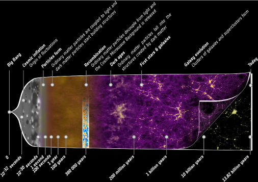
Fig. 2.1: A schematic diagram of the history of the Universe, taken from [41]. The accelerated expansion that the Universe is currently experiencing, due to Dark Energy, is not depicted in this diagram.

2.3 $\Lambda$CDM

All of what has been talked about so far forms part of the current standard model of Cosmology. However, to complete the model, we need to consider the effects of reionization. Reionization amounts to the partial ionization of the primordial gas from starlight produced by the first stars (the so-called Population III stars). The affect that reionization has on the matter in the Universe at early times is captured by using the optical depth

$$\tau(t)\equiv\sigma_{T}\int_{t}^{t_{0}}n_{e}(t)\,\mathrm{d}t$$ (2.43)

where $n_{e}$ is the number density of free electrons and $\sigma_{T}$ is the Thomson scattering cross-section. With this definition, the probability that a photon that is observed now that was emitted between the time of recombination and reionization, at a time $t$, has traveled freely is $e^{-\tau(t)}$, with the value being practically constant for emission times between recombination and reionization. When combined with other data, the data obtained from the Planck spacecraft [40] yields values for the practically constant optical depth and the redshift at which reionization occurred (assuming it was sudden) of

$$\tau=0.066\pm 0.012$$ (2.44)

$$z_{\textrm{reion}}=8.8^{+1.2}_{-1.1}$$ (2.45)

The final piece of the standard model concerns the small perturbations in the cosmic fluid density that existed in the early Universe. On large scales, the Universe is homogeneous and isotropic. However, on smaller scales, it is clear that this is violated, as the Universe contains planets, galaxies, empty space etc. Therefore, there must have existed some small differences in the density of the cosmic fluid at very early times, which then grew under the influence of gravity and the Hubble flow. These tiny perturbations present themselves in the CMB, as anisotropies in the average temperature of the microwave radiation. The Planck spacecraft made precise all-sky measurements of the CMB, which is displayed in Fig. 2.2.

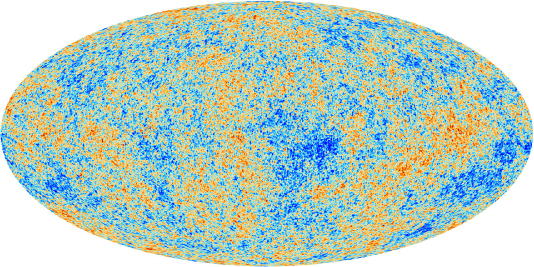
Fig. 2.2: A Mollweide projection of the CMB in galactic coordinates, as observed by the Planck spacecraft. Temperature perturbations are depicted, with $\frac{\Delta T}{T}\!\sim\!10^{-5}$. Taken from [42].

A crucial concept in early Universe Cosmology is that of the Primordial Curvature Perturbation, labeled as $\boldsymbol{\zeta}$. This will be discussed more fully in Section 3.2.1. However, we will briefly discuss two aspects of it here. The spectrum, $\mathcal{P}_{\zeta}(k)$, of the curvature perturbation conveys how much power is in the perturbation as a function of scale $k$. We also have the spectral index, $n_{s}$, which tells us how the spectrum varies with scale $k$. (The subscript $s$ denotes that this is for a scalar perturbation.) The spectral index is defined as

$$n_{s}-1\equiv\frac{\mathrm{d}\ln{(\mathcal{P}_{\zeta}(k))}}{\mathrm{d}\ln{(k)}}$$ (2.46)

with $n_{s}-1$ being referred to as the tilt of the spectrum. For constant spectral index, $\mathcal{P}_{\zeta}(k)\!\propto\!k^{n_{s}-1}$. $\mathcal{P}_{\zeta}$ is scale invariant for $n_{s}\!=\!1$. In general, $n_{s}\!=\!n_{s}(k)$, with cosmic inflation predicting $n_{s}$ close but not exactly equal to unity, so that the spectrum is approximately (but not quite) scale invariant. The Planck spacecraft made measurements of the spectrum at what is known as the pivot scale, which is $k_{0}\!\equiv\!0.002\ \mbox{Mpc${}^{-1}$}$. When combined with other data, the data obtained from the Planck spacecraft [40] yields values for the spectrum and spectral index of

$$\mathcal{P}_{\zeta}(k_{0})=(2.142\pm 0.049)\times 10^{-9}$$ (2.47)

$$n_{s}=0.9667\pm 0.0040$$ (2.48)

Lastly, we say a few words about the nature of the dark matter and the dark energy. From calculations and observations, the dark matter must be in the form of CDM, Cold Dark Matter. A CDM particle is cold in that it has negligible (meaning non-relativistic) random motion. It has negligible interaction with other particles and also negligible self-interaction, hence must be non-baryonic, with its only real presence being observed via its gravitational effect on galactic dynamics. Regarding dark energy, the simplest realization is a Cosmological Constant, denoted by $\Lambda$. This is a spatially and temporally constant term that is added to Einstein’s Field Equation, having the effect of negative pressure.
Taking all of our discussion so far into account, we are presented with the $\boldsymbol{\Lambda}$CDM model as our Concordance Model of Cosmology, which contains just six independent parameters: $\boldsymbol{H_{0}}$, $\boldsymbol{\Omega_{\textrm{{B}}}}$, $\boldsymbol{\Omega_{\textrm{{CDM}}}}$, $\boldsymbol{\tau}$, $\boldsymbol{\mathcal{P}_{\zeta}(k_{0})}$ and $\boldsymbol{n_{s}}$. Fig. 2.3 shows a plot of the agreement between the $\Lambda$CDM model and the data obtained from the Planck spacecraft.

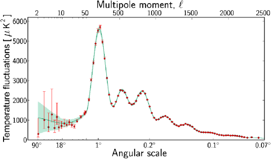
Fig. 2.3: Analysis of $\frac{\Delta T}{T}$ of the CMB in spherical harmonics, as observed by the Planck spacecraft. Red Points: Planck Data.  Green Curve: Best Fit of $\Lambda$CDM Model to Planck Data.  Light Blue Shading: Predictions of all Variations of $\Lambda$CDM Model that Best Agree with Planck Data. Taken from [43].

Chapter 3 Particle Cosmology

So far, we have been concentrating on the $\Lambda$CDM model of the Universe. We are now going to discuss Particle Cosmology, which is the field concerned with a particle physics description of the (early) Universe. The temperature and energy scales that were dominant during the very early Universe were such that Quantum Field Theory is required for a complete description of that period.

3.1 Problems of Big Bang Cosmology

As already discussed, the Big Bang Theory is hugely successful in explaining many of the properties and features that we observe in our Universe. However, it will become clear that it is not a sufficient theory on its own to explain everything that we observe. There are five main problems with the Big Bang and each of these will be discussed now. We will then see in Section 3.2 how the theory of Inflation can solve these problems.

3.1.1 Horizon Problem

With the definition of the Hubble parameter being $H\!\equiv\!\frac{\dot{a}}{a}$, we define the horizon as the distance that light (information) can travel within one Hubble Time $H^{-1}$.
We define the comoving Particle Horizon as

$$x_{\textrm{PH}}(t) \equiv\int_{0}^{t}\frac{1}{a(t)}\,\mathrm{d}t$$ (3.1)

$$=\eta(t)-\eta(0)$$ (3.2)

$$x_{\textrm{PH}}(a) =\int_{0}^{a}\frac{1}{a^{2}H}\,\mathrm{d}a$$ (3.3)

with the third line coming from the fact that we take $\dot{a}(t)\!>\!0$ (i.e. the Universe is expanding). This is the maximum distance that light (information) could have traveled since the birth of the Universe at $t,a\!=\!0$. Any two events that are separated by a distance of more than twice the particle horizon are out of casual contact. The Particle Horizon in physical coordinates is given by

$$a(t)x_{\textrm{PH}}(t) \equiv a(t)\int_{0}^{t}\frac{1}{a(t^{\prime})}\,\mathrm{d}t^{\prime}$$ (3.4)

$$a(t)x_{\textrm{PH}}(a) =a(t)\int_{0}^{a}\frac{1}{a^{2}H}\,\mathrm{d}a$$ (3.5)

We make another definition, the comoving Event Horizon, as

$$x_{\textrm{EH}}(t) \equiv\int_{t}^{\infty}\frac{1}{a(t)}\,\mathrm{d}t$$ (3.6)

$$=\eta(\infty)-\eta(t)$$ (3.7)

$$x_{\textrm{EH}}(a) =\int_{a}^{\infty}\frac{1}{a^{2}H}\,\mathrm{d}a$$ (3.8)

again with the third line coming from the fact that we take $\dot{a}(t)\!>\!0$. This is the maximum distance that light (information) can travel in the (infinite) future. An event that occurs at a spacetime point cannot influence an event at a future spacetime point if the latter is outside of the former’s event horizon. The Event Horizon in physical coordinates is given by

$$a(t)x_{\textrm{EH}}(t) \equiv a(t)\int_{t}^{\infty}\frac{1}{a(t^{\prime})}\,\mathrm{d}t^{\prime}$$ (3.9)

$$a(t)x_{\textrm{EH}}(a) =a(t)\int_{a}^{\infty}\frac{1}{a^{2}H}\,\mathrm{d}a$$ (3.10)

In reality, Eqs. 3.5 and 3.10 are definitions that use unrealistic boundary conditions, as $a\!=\!0,\infty$ is unphysical. Therefore, we usually calculate particle and event horizons between two well-defined limits

$$a(t)x_{\textrm{PH}}(a_{1},a)=a(t)\int_{a_{1}}^{a}\frac{1}{a^{2}H}\,\mathrm{d}a\hskip 50.00008pta(t)x_{\textrm{EH}}(a,a_{2})=a(t)\int_{a}^{a_{2}}\frac{1}{a^{2}H}\,\mathrm{d}a$$ (3.11)

with $a\!\gg\!a_{1}$ or $a\!\ll\!a_{2}$.
The Horizon Problem arises when we consider how the horizon of various places in the observable Universe has varied over the lifetime of the Universe and then compare this with observation. Our observable Universe is statistically homogeneous and isotropic on cosmological scales. One manifestation of this is that of the large isotropy that exists in the CMB. Over the entire sky, the temperature of the CMB is the same to within 1 part in $\sim\!10^{5}$. Therefore, it is very safe to assume that all parts of the CMB were in thermal equilibrium with each other at the time of last scattering and thus were in casual contact with each other. However, when we consider two parts of the CMB that are separated by more than a few degrees across the sky, we find that the particle horizon’s of these two parts do not overlap. Therefore, they have never been in casual contact with each other, as there has not been enough time for light (information) to travel between the two parts given the age of the Universe. The Horizon Problem is thus to explain how each part of the observable Universe is so extremely statistically similar to every other part, given that the vast majority of parts have never been in casual contact with each other.

3.1.2 Flatness Problem

From looking at Eq. 2.29 regarding the Density Parameter, we see that as time evolves from the birth of the Universe, i.e. as $\dot{a}^{2}$ decreases rapidly, $\Omega$ grows rapidly, away from a value of 1. We observe for the Density Parameter the current value $\Omega_{0}\!=\!1.000\pm 0.005$ (LABEL:Eq.:_Omega_{0}), which is very close to 1, i.e. a spatially flat Universe. Therefore, in the past, the value must have been even more precisely close to 1, with it having had a value of 1 to a precision of at least $\sim\!10^{-62}$ around the Planck time. This Flatness Problem is thus a fine-tuning problem for the initial conditions of the Universe.
The Flatness Problem, when looked at from a slightly different viewpoint, can also be regarded as an Age Problem. If the value of $\Omega$ had been only slightly larger than it appears to have been, then the Universe would have been of a sufficient density that it would have collapsed at a time much sooner than the age of our observable Universe. If, on the other hand, the value of $\Omega$ had been only slightly smaller than it appears to have been, then the Universe would have expanded too quickly for stars and galaxies to have formed the LSS that we observe today. Therefore, the fine-tuning problem can be regarded as an Age Problem, in that how has our observable Universe become as old as it is?

3.1.3 Relic Problem

In contrast to the two problems already mentioned, the Relic Problem is not specific to a Hot Big Bang model of the Universe, but rather something that has to be considered within the total picture of Particle Cosmology. There exist a large variety of particle physics models and applications of these to Cosmology that have the ability to produce many types of relic; particles and other components that contradict established theory and/or observation, such as gravitinos coming from SUGRA and moduli coming from string theory. Another example, which was the subject of the original work of Alan Guth on inflation [44], considered the effect of magnetic monopole creation during a GUT phase transition in the very early Universe. Any monopoles that are produced in the very early Universe must neither spoil the success of BBN nor be in direct tension with observations of such particles. An abundant creation of monopoles in the early Universe would have the affect of overclosing the Universe. Therefore, we must have the situation where either any such model of the very early Universe does not produce too many relics or there must exist some mechanism such that these are not in conflict with our observations, such as having them be diluted away somehow.

3.1.4 Baryon Asymmetry Problem

It is clear that there exist many more particles than anti-particles in the Universe. However, there is no explicit mechanism in the Hot Big Bang model itself that can account for this Baryon Asymmetry and according to the model, identically equal amounts of matter and anti-matter should have been created in the early Universe.

3.1.5 Initial Perturbation/Structure Problem

Lastly, there is the issue of the creation of the LSS of the observable Universe. Assuming just an expanding FLRW Universe, there arises the question of how the observable structure in the Universe came into existence, as this expanding spacetime is exactly homogeneous and isotropic. Although our observable Universe is highly homogeneous and isotropic on cosmological scales, it is clear that this must break down at some level, in order to facilitate the existence of stars, galaxies and humans! In addition, when we look at the CMB, we see tiny perturbations in the temperature across the sky. What mechanism was responsible for producing the associated density perturbations in the very early Universe?

3.2 Cosmic Inflation

We now discuss one of the key areas of Particle Cosmology in the 21^st century and indeed the main topic of work in this thesis: Cosmic Inflation. Firstly, let us define inflation. With regard to the scale factor $a(t)$, inflation is defined as any period of spacetime expansion in which we have

$$\ddot{a}>0$$ (3.12)

We therefore have a period of “repulsive gravity”. Another, extremely important, definition of inflation is

$$\frac{\mathrm{d}}{\mathrm{d}t}\frac{H^{-1}}{a}<0$$ (3.13)

This defines inflation as a period of expansion in which the comoving Hubble length is decreasing. Another definition of inflation, in terms of the time evolution of the Hubble parameter, is

$$-\frac{\dot{H}}{H^{2}}<1$$ (3.14)

As this inequality becomes stronger, $H$ becomes more and more constant during the period of inflation, with the expansion becoming more and more exponential, i.e. $a\!\propto\!e^{Ht}$. It should be noted that Eqs. 3.12, 3.13 and 3.14 are all equivalent.
If we now include GR in our discussion, we have one final definition of inflation. Using the (Friedmann) Acceleration Equation, Eq. 2.20, we have

$$\rho+3P<0$$ (3.15)

This implies that we require negative enough pressure (“repulsive gravity”), $P\!<\!-\frac{\rho}{3}$, in order to achieve a period of inflation.
Now we will discuss how a period of inflation can solve the five problems of an isolated Big Bang Cosmology mentioned above. Firstly, the Horizon Problem. The solution to this problem is to say that the entire observable Universe used to be inside the horizon, prior to the end of inflation. During inflation however, different scales of relevance to our observable Universe were “stretched” to outside of the horizon at different times, remembering that one of the definitions of inflation is that of a decreasing comoving Hubble length, Eq. 3.13. At later times, after inflation, these scales then started to re-enter the horizon, again at different times for different scales.
Now, the Flatness Problem. From looking at Eq. 2.29 regarding the Density Parameter, we can see that the RHS will tend towards 0 during inflation. The reason for this, is that during inflation $\ddot{a}\!>\!0$ by definition. Therefore, $\dot{a}^{2}$ will grow rapidly, which will have the affect of rapidly driving the value of $\Omega$ towards 1 throughout the entire period of inflation. However, for the problem to be solved sufficiently, we require that the entire observable Universe is well within the horizon, $aH\!\ll\!H_{0}$, a long time before cosmological scales exit the horizon during inflation.
We now discuss the solution to the Relic Problem. Any relics that exist before or during inflation will be rapidly diluted away by the inflation. They will quickly become non-interacting as their number density decreases, due to the rapid expansion, as the interaction rates quickly fall below $H$. However, we may still have relics that are produced thermally after the end of inflation. This will depend mainly on the reheat temperature of the Universe after the end of inflation. Therefore, to avoid specific types of relics that may be an issue, for example in how they spoil BBN, any particular model of inflation must have a reheat temperature low enough so as to not produce an unacceptable amount of such relics. Alternatively, a second period of inflation, known as Thermal Inflation (see Chapter 4), can affectively eradicate them.
Let us now discuss the Baryon Asymmetry Problem. Inflation can accommodate Baryogenesis mechanisms that produce the asymmetry between matter and anti-matter. In order to achieve Baryogenesis, we require the following conditions, known as the Sakharov Conditions

1. Violation of B (Baryon Number) conservation

2. Violation of CP symmetry

3. Absence of thermal equilibrium

It is the last of these conditions that can be achieved during a period of inflation.
Lastly, regarding the problem of how initial perturbations were seeded that gave rise to the LSS that we observe, inflation naturally produces such perturbations that can indeed give rise to the structure that we see in our observable Universe. This is because inflation generates the required primordial curvature perturbation, which we will now discuss. (A much more detailed discussion is found in Section 3.2.3).

3.2.1 $\delta N$ Formalism

We now go on to define a crucial quantity known as the Primordial Curvature Perturbation, $\zeta$. We will then see how we can use the so-called $\delta N$ formalism to calculate this. Let us consider a coordinate gauge in which the spatial threads are comoving and the temporal slices are such that each one has a uniform energy density. The spatial part of the spacetime metric is

$$g_{ij}=a^{2}(\textbf{x},t)\gamma_{ij}(\textbf{x})$$ (3.16)

where we have

$$a(\textbf{x},t)\equiv a(t)e^{\zeta(\textbf{x},t)}$$ (3.17)

and

$$\gamma_{ij}(\textbf{x})\equiv\left(\textbf{I}e^{2h(\textbf{x})}\right)_{ij}$$ (3.18)

where $h(\textbf{x})$ is the primordial tensor perturbation. We therefore have as our definition of $\zeta$

$$\zeta(\textbf{x},t)\equiv\ln{\left(\frac{a(\textbf{x},t)}{a(t)}\right)}$$ (3.19)

Now let us consider a generic coordinate gauge, in which we still have a comoving threading but a generic slicing, as opposed to one in which each slice has a uniform energy density. We have

$$\tilde{g}_{ij}=\tilde{a}^{2}(\textbf{x},t)\tilde{\gamma}_{ij}(\textbf{x})$$ (3.20)

where

$$\tilde{a}(\textbf{x},t)\equiv a(t)e^{\psi(\textbf{x},t)}$$ (3.21)

and

$$\tilde{\gamma}_{ij}(\textbf{x})\equiv\left(\textbf{I}e^{2\tilde{h}(\textbf{x})}\right)_{ij}$$ (3.22)

At any given value of $t$, the scale factors $a(\textbf{x},t)$ and $\tilde{a}(\textbf{x},t)$ differ only because of the difference in the time coordinate of the two spacetime slices. Therefore, in order to maintain generality, we will drop the ~ on the scale factor. We can define a quantity called the e-folding number as

$$N\equiv\ln{\left(\frac{a_{2}}{a_{1}}\right)}$$ (3.23)

which is the number of exponential expansions of the Universe between when the scale factor is $a_{1}$ and when it is $a_{2}$. As $H\!\equiv\!\frac{\dot{a}}{a}$, this can also be expressed as

$$N=\int_{t_{1}}^{t_{2}}H\,\mathrm{d}t$$ (3.24)

and is thus sometimes called the number of Hubble times. The difference in the number of e-foldings between any two generic spacetime slices is given by

$$\delta N(\textbf{x}) =\delta\int_{t_{1}}^{t_{2}}\frac{1}{a(\textbf{x},t)}\frac{\mathrm{d}a(\textbf{x},t)}{\mathrm{d}t}\,\mathrm{d}t$$ (3.25)

$$=\psi(\textbf{x},t_{2})-\psi(\textbf{x},t_{1})$$ (3.26)

We will define what we will call a flat spacetime slice as the one where

$$\psi(\textbf{x},t)=0$$ (3.27)

We define the term $\delta N(\textbf{x},t)$ to denote the number of e-foldings between the flat slice and a slice of uniform energy density at time $t$. Therefore, we reach what is called the $\delta N$ formalism

$$\zeta(\textbf{x},t)=\delta N(\textbf{x},t)$$ (3.28)

which thus allows us to calculate the primordial curvature perturbation from calculating the difference in the number of e-foldings of expansion between a flat slice and a latter uniform energy density slice, which is extremely useful when considering the perturbation that is produced from a particular inflation model.

3.2.2 Scalar Fields

Inflation models most often assume that the content of the Universe during and immediately after inflation is dominated by the presence of one or more scalar fields, $\phi_{n}$. A scalar field is homogeneous (being as it is homogenized by inflation) and will behave like a perfect fluid, as its stress is isotropic.
Let us consider the contents of the Universe to simply be a single scalar field, $\phi$. The action that governs this scenario is

$$S=\int\sqrt{-g}\left(\frac{1}{2}M_{P}^{2}R+\mathcal{L}\right)\,\mathrm{d^{4}}\!x$$ (3.29)

where $g$ is the determinant of the metric tensor $g_{\mu\nu}$, $R$ is the Ricci scalar and $\mathcal{L}$ is the Lagrangian density of the scalar field, which is

$$\mathcal{L}=-\frac{1}{2}\partial^{\mu}\phi\partial_{\mu}\phi-V(\phi)$$ (3.30)

where the first term is called the kinetic term and the second term is called the scalar field potential. By using the action principle, $\delta S\!=\!0$, we can obtain the Energy-Momentum tensor for the scalar field, which is

$$T_{\mu\nu}=-2\frac{\partial\mathcal{L}}{\partial g^{\mu\nu}}+g_{\mu\nu}\mathcal{L}$$ (3.31)

Substituting Eq. 3.30 into here gives

$$T^{\mu}_{\nu}=\partial^{\mu}\phi\partial_{\nu}\phi-\delta^{\mu}_{\nu}\left(\frac{1}{2}\partial^{\alpha}\phi\partial_{\alpha}\phi+V(\phi)\right)$$ (3.32)

The “$00$” (“$tt$”) component of this Energy-Momentum tensor gives the energy density for a homogeneous scalar field, which is

$$T^{0}_{0}=\rho=\frac{1}{2}\dot{\phi}^{2}+V(\phi)$$ (3.33)

and the $T^{1}_{1}\!=\!T^{2}_{2}\!=\!T^{3}_{3}$ components give the pressure for a homogeneous scalar field, which is

$$P=\frac{1}{2}\dot{\phi}^{2}-V(\phi)$$ (3.34)

For simplicity, let us continue to assume that the cosmological fluid during and immediately after inflation consists principally of just the one scalar field, $\phi$. If the kinetic energy density term of this field, $\frac{1}{2}\dot{\phi}^{2}$, is small, i.e. if the field varies slowly, or not at all, then we will have a situation in which

$$P\approx-\rho$$ (3.35)

Therefore, the equation of state will be

$$w=\frac{P}{\rho}\approx-1$$ (3.36)

and we will therefore have a period of (quasi-de Sitter) inflation, in which the scale factor goes (nearly) like $a(t)\!\propto\!e^{Ht}$ (see Section 2.1.1). As $\phi$ is the component in the cosmological fluid that is responsible for driving inflation, we call the field, as well as its associated particle within the context of QFT, the Inflaton.

3.2.3 Particle Production

We now briefly discuss the method by which we actually obtain an energy density perturbation from a scalar field. During inflation, the inflaton field $\phi$ will naturally acquire quantum fluctuations, $\delta\phi$, as a direct result of the uncertainty principle. We assume that $\phi$ is in a vacuum state and so we have 0 particles as the eigenvalue of the number operator. The field equation of the first-order perturbation $\delta\phi$ is

$$\ddot{\delta\phi}_{\textbf{k}}+3H\dot{\delta\phi}_{\textbf{k}}+\left(\frac{k}{a}\right)^{2}\delta\phi_{\textbf{k}}+V^{\prime\prime}\delta\phi_{\textbf{k}}=0$$ (3.37)

where $\phi_{\textbf{k}}$ is the Fourier transform of $\phi(\textbf{x})$

$$\phi_{\textbf{k}}=\frac{1}{(2\pi)^{\frac{2}{3}}}\int\phi(\textbf{x})e^{-i\textbf{k}\cdot\textbf{x}}\,\mathrm{d^{3}}\!x$$ (3.38)

We concern ourselves only with a light field. Given this, we have

$$V^{\prime\prime}\ll\left(\frac{k}{a}\right)^{2}$$ (3.39)

Therefore, we have the field equation

$$\ddot{\delta\phi}_{\textbf{k}}+3H\dot{\delta\phi}_{\textbf{k}}+\left(\frac{k}{a}\right)^{2}\delta\phi_{\textbf{k}}\simeq 0$$ (3.40)

As the key interest in this discussion is the time around horizon exit, let us concentrate on this and so let us set

$$H=H_{\ast}$$ (3.41)

where $H_{\ast}$ is the scale-independent constant value of $H$ at around the time of horizon exit. The use of the constant value $H_{\ast}$ as opposed to the scale-dependent value $H_{k}$, for when the scale $k$ exits the horizon, is an approximation, used to simplify the derivation here. The approximation is valid, as in quasi-de Sitter inflation we have $H\!\approx\!constant$, i.e. $H$ varies extremely slowly with scale. We now transform from cosmic time $t$ to conformal time

$$\eta=-\frac{1}{aH_{\ast}}$$ (3.42)

and also consider instead the comoving field perturbation

$$\varphi\equiv a\delta\phi$$ (3.43)

Eq. 3.40 now becomes

$$\frac{\mathrm{d^{2}}\varphi_{\textbf{k}}(\eta)}{\mathrm{d}\eta^{2}}+\omega_{k}^{2}(\eta)\varphi_{\textbf{k}}(\eta)=0$$ (3.44)

where

$$\omega_{k}^{2}(\eta)=k^{2}-\frac{2}{\eta^{2}}$$ (3.45)

where we have assumed $a(t)\!\propto\!e^{Ht}$. We have thus obtained a harmonic oscillator scenario. Following the usual procedure of QFT, we will now promote variables to operators and quantize this harmonic oscillator. We express the comoving perturbation in terms of Fourier components as

$$\hat{\varphi}_{\textbf{k}}(\eta)=\varphi_{k}(\eta)\hat{a}(\textbf{k})+\varphi_{k}^{\ast}(\eta)\hat{a}^{\dagger}(-\textbf{k})$$ (3.46)

where $\hat{a}^{\dagger}$ and $\hat{a}$ are creation and annihilation operators respectively, that satisfy

$$\left[\hat{a}(\textbf{k}),\hat{a}^{\dagger}(\textbf{k}^{\prime})\right]=(2\pi)^{3}\delta^{3}\!\left(\textbf{k}-\textbf{k}^{\prime}\right)$$ (3.47)

and

$$\left[\hat{a}(\textbf{k}),\hat{a}(\textbf{k}^{\prime})\right]=0$$ (3.48)

We assume that the vacuum state is that of the Bunch-Davies vacuum. This vacuum state is the ground state of the system within a curved spacetime background. For very early times, as $\eta\!\to\!-\infty$, the Bunch-Davies vacuum gives the initial condition

$$\varphi_{k}(\eta)=\frac{1}{\sqrt{2k}}e^{-ik\eta}$$ (3.49)

As this is for very early times, it also corresponds to very small wavelengths and so corresponds to the Minkowski vacuum, i.e. the vacuum of the system within a flat spacetime background. The solution for $\varphi_{k}(\eta)$ is

$$\varphi_{k}(\eta)=\frac{(k\eta-i)}{k\eta}\frac{e^{-ik\eta}}{\sqrt{2k}}$$ (3.50)

which is the mode function for the Bunch-Davies vacuum. The spectrum is given by

$$\left\langle\hat{\varphi}_{\textbf{k}}\hat{\varphi}_{\textbf{k}^{\prime}}\right\rangle=\frac{1}{4\pi k^{3}}\mathcal{P}_{\varphi}(k)\delta^{3}\!\left(\textbf{k}+\textbf{k}^{\prime}\right)$$ (3.51)

Substituting Eq. 3.46 and the commutation relations Eqs. 3.47 and 3.48 into Eq. 3.51 yields

$$\mathcal{P}_{\varphi}(k,\eta)=\frac{k^{3}}{2\pi^{2}}|\varphi_{k}(\eta)|^{2}$$ (3.52)

Substituting LABEL:Eq.:_varphi_{k}(eta)_Solution into this, dividing by $a^{2}$ (to return back to the $\delta\phi$ perturbations) and evaluating it a few Hubble times after horizon exit gives the time-independent result

$$\mathcal{P}_{\delta\phi}(k)=\left(\frac{H_{\ast}}{2\pi}\right)^{2}$$ (3.53)

which is the Hawking Temperature for de Sitter spacetime. See [45] for the original derivation of this result.
Now let us consider a time well after horizon exit. The solution for $\varphi_{k}(\eta)$, LABEL:Eq.:_varphi_{k}(eta)_Solution, tends to

$$\varphi_{k}(\eta)\to\frac{-i}{k\eta\sqrt{2k}}$$ (3.54)

i.e. a purely imaginary solution. Eq. 3.46 now becomes

$$\hat{\varphi}_{\textbf{k}}(t)=\varphi_{k}(t)\left(\hat{a}(\textbf{k})-\hat{a}^{\dagger}(-\textbf{k})\right)$$ (3.55)

Therefore, we can see that, before horizon exit, the perturbation $\varphi_{\textbf{k}}$ of the scalar field $\phi$ is a quantum object. However, well after horizon exit, the perturbation has become an almost scale-invariant classical perturbation. The classical perturbation is conserved whilst outside the horizon [46].
After the end of inflation, there must exist a mechanism for transferring the energy density of $\phi$ into the components that will initiate the Hot Big Bang. This mechanism is called Reheating. At around the time of horizon entry, the classical perturbation starts to oscillate and thus we have a particle interpretation for $\phi$ within the context of QFT. Reheating can be sudden or take some cosmic time to complete and is complete when we have a cosmic fluid whose components are radiation (i.e. relativistic), which are all in thermal equilibrium with each other and that this fluid is the initiation of the Hot Big Bang. Reheating is typically complete when the Hubble parameter $H$ has fallen to the same order as the decay rate of the $\phi$ field

$$H\sim\Gamma_{\phi}$$ (3.56)

The temperature at the point where reheating is complete is known as the Reheat Temperature and is given by

$$T_{\textrm{reh}}\sim\sqrt{M_{P}\Gamma_{\phi}}$$ (3.57)

There also exists the possibility of having a period of Preheating. This is where most of the energy density of the inflaton decays immediately (explosively) into radiation, due to non-perturbative effects. However, preheating is typically incomplete. Therefore, the final stages of inflaton decay are perturbative. If $\Gamma_{\phi}\!\ll\!H_{\ast}$, then preheating products are irrelevant, as the energy density of the Universe becomes dominated by the oscillating inflaton again. However, if $\Gamma_{\phi}\!\lesssim\!H_{\ast}$, then the Hot Big Bang will begin after preheating.

Chapter 4 A New Thermal Inflation Model

4.1 Thermal Inflation

Thermal Inflation [47, 48, 49, 50] is a brief period of inflation (lasting about 10 e-folds) that could have occurred after a period of prior primordial inflation. It occurs due to finite-temperature effects arising from a coupling between a thermal waterfall field and the thermal bath created from the partial or complete reheating from the prior inflation. If we start with a zero-temperature scalar field theory, we can calculate the affect that placing the system in a thermal bath at temperature $T$ has on the theory by introducing an interaction term in the form of a 1-loop correction. After calculating the appropriate variables within the context of thermal field theory, we can take the high-$T$ approximation of the correction, which gives a thermal contribution $V_{\textrm{T}}\!\simeq\!g^{2}T^{2}\phi^{2}$ to the effective potential $V_{\textrm{eff}}$, where $g$ is the coupling constant of the interaction between $\phi$ and the thermal bath. This results in a thermal correction to the effective mass of $m_{\textrm{T}}^{2}\!\simeq\!g^{2}T^{2}$. Within the context of statistical mechanics, the interpretation of $V_{\textrm{eff}}$ is that of the free energy of $\phi$ when the field is in thermal equilibrium with the thermal bath at temperature $T$, with the minima in $V_{\textrm{eff}}$ defining the equilibrium states, with $\left\langle\phi\right\rangle$ representing the thermal average, as opposed to the vacuum expectation value (VEV).
Let us take the following potential

$$V(\phi,T)=V_{0}+\left(g^{2}T^{2}-\frac{1}{2}m_{0}^{2}\right)\phi^{2}+\lambda\frac{\phi^{6}}{M_{P}^{2}}$$ (4.1)

Initially, the temperature of the Universe will be sufficiently high that the temperature term in the brackets will be greater than the mass term in the brackets. This will have the affect of holding the $\phi$ field at $\phi\!=0$. When the energy density of the Universe falls below the value of $V_{0}$ in the thermal inflation potential, the $V_{0}$ term will come to dominate the energy density of the Universe and thermal inflation will begin. It will continue until very shortly after the point when the temperature term has become smaller than the mass term, at which point spontaneous symmetry breaking will occur and so $\phi$ will start to roll down the potential towards either the positive or negative VEV. The shape of the potential in this scenario is displayed in Fig. 4.1.

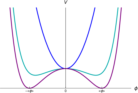
Fig. 4.1: Blue: $T\!>\!\frac{m_{0}}{\sqrt{2}g}$   Cyan: $T\!<\!\frac{m_{0}}{\sqrt{2}g}$   Purple: $T\!=\!0$

This scenario is quite general and would not be particularly unexpected in the early Universe. However, Thermal Inflation was originally proposed as a solution to the moduli problem [47, 48]. Moduli are scalar fields that arise in string theory. They are flaton fields, which are flat directions in SUSY. These have no tree-level terms in the potential from SUSY and they get a mass term from SUSY breaking (they do not have a quartic (self-interaction) term). Flaton fields have nearly flat potentials (with $\sqrt{V^{\prime\prime}}$ being the relevant quantity, with a prime indicating the (partial) derivative of $V$ with respect to the flaton field) and large VEVs, $\sim\!M_{P}$. The problem is that when inflation ends and a modulus starts to oscillate around its large VEV, the oscillations will also be very large and the energy density of the moduli will start to dominate the energy density of the Universe. This has the affect of creating an abundance of moduli particles that are long-lived and do not decay prior to BBN, thus creating unwanted relics. Thermal Inflation alleviates this problem by diluting away the moduli during the period of inflation. They are not re-created in abundance after thermal inflation, as the typical energy scales involved after thermal inflation are much lower than those typical of a prior period of inflation.

4.2 The Model

It is possible for the mass of a certain scalar field to be dependent on another scalar field [27, 28, 31, 38, 13, 25, 26, 32, 33, 34, 39, 22]. More specifically, the mass of a thermal waterfall field that is responsible for a bout of thermal inflation could be dependent on another scalar field. If the latter is light during primordial inflation, quantum fluctuations of the field are converted to almost scale-invariant classical field perturbations at around the time of horizon exit. If the scalar field remains light all the way up to the end of thermal inflation, then thermal inflation will end at different times in different parts of the Universe, because the value of the spectator field determines the mass of the thermal waterfall field, which in turn determines the end of thermal inflation. This is the “end of inflation” mechanism [31] and it will generate a contribution to the primordial curvature perturbation $\zeta$. In addition to this, if the scalar field remains light up until the decay of the thermal waterfall field, the decay rate of the thermal waterfall field will be modulated, due to the mass of the thermal waterfall field (which controls the decay rate) being dependent on the light scalar field. The decay of the thermal waterfall field will generate a second contribution to $\zeta$. The motivation of this work is to explore these two scenarios to see if either of them can produce the dominant contribution to the primordial curvature perturbation with characteristic observational signatures. We consider that these are the dominant contributions to the curvature perturbation, so that the inflaton’s contribution can be ignored.
It should be noted that the first scenario is very similar to that in Ref. [30]. However, in that paper the authors use a modulated coupling constant rather than a modulated mass. Also, the treatment that has been given to the work in this thesis is much more comprehensive. One example of this is in the consideration of the effect that the thermal fluctuation of the thermal waterfall field has on the model (see Section 4.4.3.6). Another example is the requirement that the thermal waterfall field is thermalized (see Section 4.4.3.7). Also, there is no consideration given in Ref. [30] to requiring a fast transition from thermal inflation to thermal waterfall field oscillation (see Section 4.4.3.10), as detailed in Ref. [34], as this paper appeared after Ref. [30].
Throughout this work, units are used where $c\!=\!\hbar\!=\!k_{B}\!=\!1$ and the reduced Planck Mass is $M_{P}\!=\!2.436\times 10^{18}\ \mbox{GeV}$.
The potential that is considered in this model is

$$V(\phi,T,\psi)=V_{0}+\left(g^{2}T^{2}-\frac{1}{2}m_{0}^{2}+h^{2}\frac{\psi^{2\alpha}}{M_{P}^{2\alpha-2}}\right)\phi^{2}+\lambda\frac{\phi^{2n+4}}{M_{P}^{2n}}+\frac{1}{2}m_{\psi}^{2}\psi^{2}$$ (4.2)

where $\phi$ is the thermal waterfall scalar field, $\psi$ is a light spectator scalar field, $T$ is the temperature of the thermal bath, $g$, $h$ and $\lambda$ are dimensionless coupling constants, $\alpha\geq 1$ and $n\geq 1$ are integers and the $-\frac{1}{2}m_{0}^{2}$ and $\frac{1}{2}m_{\psi}^{2}$ terms come from soft SUSY breaking. We do not include a $\phi^{4}$ term, because the thermal waterfall field is a flaton, whose potential is stabilised by the higher-order non-renormalizable term.
We make the following definition

$$m^{2}\equiv m_{0}^{2}-2h^{2}\frac{\psi^{2\alpha}}{M_{P}^{2\alpha-2}}$$ (4.3)

i.e. we combine the bare mass and coupling term into a new mass quantity. The variation of $m$, which is due only to the variation of $\psi$, is

$$\delta m=-\frac{2\alpha h^{2}\psi^{2\alpha-1}}{mM_{P}^{2\alpha-2}}\delta\psi$$ (4.4)

We only consider the case where the mass of $\phi$ is coupled to one field. If the mass were coupled to several similar fields, the results are just multiplied by the number of fields. If the multiple fields are different, then there will be only a small number that dominate the contribution to the mass perturbation. Therefore we consider only one for simplicity.
Using Eq. 4.3, our redefined mass quantity, the potential becomes

$$V(\phi,T,\psi)=V_{0}+\left(g^{2}T^{2}-\frac{1}{2}m^{2}\right)\phi^{2}+\lambda\frac{\phi^{2n+4}}{M_{P}^{2n}}+\frac{1}{2}m_{\psi}^{2}\psi^{2}$$ (4.5)

This potential is shown in Fig. 4.2.

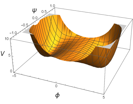
Arbitrary Units

Fig. 4.2: The potential given by Eq. 4.5.

It would appear from the potential that domain walls will be produced, due to the fact that in some parts of the Universe $\phi$ will roll down to $+\left\langle\phi\right\rangle$ while in others parts it will roll down to $-\left\langle\phi\right\rangle$. However, this does not occur, as we can interpret $\phi$ as being the real part of a complex field whose potential contains only one continuous VEV.
The zero temperature potential is

$$V(\phi,0,\psi)=V_{0}-\frac{1}{2}m^{2}\phi^{2}+\lambda\frac{\phi^{2n+4}}{M_{P}^{2n}}+\frac{1}{2}m_{\psi}^{2}\psi^{2}$$ (4.6)

To obtain the VEV of $\phi$, we find the minimum of the zero temperature potential. The VEV is

$$\left\langle\phi\right\rangle=\left(\frac{mM_{P}^{n}}{\sqrt{\left(2n+4\right)\lambda}}\right)^{\frac{1}{n+1}}$$ (4.7)

$V\!=\!0$ at the VEV. $V_{0}$ is obtained by inserting the VEV into the zero temperature potential and then looking along the $\psi\!=\!0$ direction. We obtain

$$V_{0}\sim\left(\frac{m_{0}^{2n+4}M_{P}^{2n}}{\lambda}\right)^{\frac{1}{n+1}}$$ (4.8)

We use the Friedmann equation

$$M_{P}^{2}H_{\textrm{TI}}^{2}\sim V_{0}$$ (4.9)

giving the energy density of the Universe during thermal inflation to obtain the Hubble parameter during thermal inflation as

$$H_{\textrm{TI}}\sim\left(\frac{m_{0}^{n+2}}{\sqrt{\lambda}\,M_{P}}\right)^{\frac{1}{n+1}}$$ (4.10)

Within this model, we will consider two cases regarding the decay rate of the inflaton, $\Gamma_{\varphi}$, with $\varphi$, the inflaton, being the field driving the period of primordial inflation prior to thermal inflation. Firstly, the case that $\Gamma_{\varphi}\!\gtrsim\!H_{\textrm{TI}}$, i.e. that reheating from primordial inflation occurs before or around the time of the start of thermal inflation. Secondly, we will consider the case that $\Gamma_{\varphi}\!\ll\!H_{\textrm{TI}}$, i.e. that reheating from primordial inflation occurs at some time after the end of thermal inflation. In the case of $\Gamma_{\varphi}\!\gtrsim\!H_{\textrm{TI}}$, thermal inflation will begin at a temperature

$$T_{1}\sim V_{0}^{\frac{1}{4}}$$ (4.11)

$T_{1}$ corresponds to the temperature when the potential energy density becomes comparable with the energy density of the thermal bath, for which the density is $\rho_{\gamma}\!\sim\!T^{4}$. In the case of $\Gamma_{\varphi}\!\ll\!H_{\textrm{TI}}$, thermal inflation will begin at a temperature

$$T_{1}\sim\left(M_{P}^{2}\,H_{\textrm{TI}}\Gamma_{\varphi}\right)^{\frac{1}{4}}$$ (4.12)

In both cases, thermal inflation ends at a temperature

$$T_{2}=\frac{m}{\sqrt{2}\,g}$$ (4.13)

$T_{2}$ corresponds to the temperature when the tachyonic mass term of the thermal waterfall field becomes equal to the thermally-induced mass term in Eq. 4.5.

4.3 $\phi$ Decay Rate, Spectral Index and Tensor Fraction

4.3.1 $\phi$ Decay Rate

The decay rate of $\phi$ is given by

$$\Gamma\sim\mathrm{max}\left\{g^{2}m_{\phi,\textrm{osc}}\hskip 5.0pt,\hskip 5.0pt\frac{m_{\phi,\textrm{osc}}^{3}}{M_{P}^{2}}\right\}$$ (4.14)

where $m_{\phi,\textrm{osc}}$ is the effective mass of $\phi$ during the time of $\phi$’s oscillations around its VEV after the end of thermal inflation. This is calculated as

$$m_{\phi,\textrm{osc}}\sim m$$ (4.15)

Therefore we obtain

$$\Gamma\sim\mathrm{max}\left\{g^{2}m\hskip 5.0pt,\hskip 5.0pt\frac{m^{3}}{M_{P}^{2}}\right\}$$ (4.16)

The first expression is for decay into the thermal bath via direct interactions and the second is for gravitational decay. We will only consider the case in which the direct decay is the dominant channel ($g$ is not taken to be very small). This is the case when

$$m\ll gM_{P}$$ (4.17)

Therefore we have just

$$\Gamma\sim g^{2}m$$ (4.18)

4.3.2 Spectral Index — $n_{s}$ and $n_{s}^{\prime}$

Thermal Inflation has the effect of changing the number of e-folds before the end of primordial inflation at which cosmological scales exit the horizon. This affects the value of the spectral index $n_{s}$ of the curvature perturbation $\zeta$, assuming $\zeta$ is generated due to the perturbations of the spectator scalar field. The spectral index is given by [1]

$$n_{s}\simeq 1-2\epsilon_{H}+2\eta_{\psi\psi}$$ (4.19)

where $\epsilon_{H}$ and $\eta_{\psi\psi}$ are slow-roll parameters, defined as

$$\epsilon_{H}\equiv 2M_{P}^{2}\left(\frac{H^{\prime}(\varphi)}{H(\varphi)}\right)^{2}$$ (4.20)

and

$$\eta_{\psi\psi}\equiv\frac{V_{\psi\psi}}{3H^{2}}$$ (4.21)

where $H^{\prime}(\varphi)$ is the derivative of the Hubble parameter with respect to the inflaton field $\varphi$ and $V_{\psi\psi}\equiv\frac{\partial^{2}V}{\partial\psi^{2}}$. $\epsilon_{H}$ and $\eta_{\psi\psi}$ are to be evaluated at the point where cosmological scales exit the horizon during primordial inflation. In the limit of slow-roll inflation, which we consider to be the case for our primordial inflation period, $\epsilon_{H}\rightarrow\epsilon$, which is defined as

$$\epsilon\equiv\frac{M_{P}^{2}}{2}\left(\frac{V^{\prime}(\varphi)}{V(\varphi)}\right)^{2}$$ (4.22)

where $V(\varphi)$ is the inflaton potential and $V^{\prime}(\varphi)$ is the derivative of that potential with respect to the inflaton field $\varphi$. $\epsilon$ is to be evaluated at the point where cosmological scales exit the horizon during primordial inflation. The spectral index now becomes

$$n_{s}\simeq 1-2\epsilon+2\eta_{\psi\psi}$$ (4.23)

Regarding the various scalar fields involved in this model, the reason why $\epsilon$ depends only on $\varphi$ is because this slow-roll parameter captures the inflationary dynamics of primordial inflation, which is governed only by $\varphi$ in our model (we are assuming that both $\psi$ and $\phi$ have settled to a constant value (LABEL:Subsubsection:_The_Field_Value_phi_{*} and LABEL:Subsubsection:_The_Field_Value_psi_{*} respectively) by the time cosmological scales exit the horizon during primordial inflation). In a similar fashion, the reason why the slow-roll parameter $\eta$ depends only on $\psi$ is because this parameter captures the dependance on the spectral index of the field(s) whose perturbations contribute to the observed primordial curvature perturbation $\zeta$. In our case, this is only the $\psi$ field.
The definition of the running of the spectral index is [1]

$$n_{s}^{\prime} \equiv\frac{\mathrm{d}n_{s}}{\mathrm{d}\ln{(k)}}$$ (4.24)

$$\simeq-\frac{\mathrm{d}n_{s}}{\mathrm{d}N}$$ (4.25)

the second line coming from $\mathrm{d}\ln{(k)}\!=\!\mathrm{d}\ln{(aH)}\!\simeq\!H\mathrm{d}t\!\equiv\!-\mathrm{d}N$, where $k\!=\!aH$. From Eq. 4.23 we have

$$n_{s}^{\prime} \simeq 2\frac{\mathrm{d}\epsilon}{\mathrm{d}N}-2\frac{\mathrm{d}\eta_{\psi\psi}}{\mathrm{d}N}$$ (4.26)

$$\simeq 2\epsilon\frac{\mathrm{d}\ln{(\epsilon)}}{\mathrm{d}N}-2\frac{\mathrm{d}\eta_{\psi\psi}}{\mathrm{d}N}$$ (4.27)

By differentiating the natural log of $\epsilon$ with respect to $N$, we obtain [1]

$$\frac{\mathrm{d}\ln{(\epsilon)}}{\mathrm{d}N}\simeq-4\epsilon+2\eta$$ (4.28)

where $\eta$ is a slow-roll parameter given by

$$\eta\equiv M_{P}^{2}\frac{V^{\prime\prime}(\varphi)}{V(\varphi)}$$ (4.29)

where $V^{\prime\prime}(\varphi)$ is the second derivative of the inflaton potential with respect to the inflaton field $\varphi$. $\eta$ is to be evaluated at the point where cosmological scales exit the horizon during primordial inflation. By differentiating $\eta_{\psi\psi}$ with respect to $N$ using the quotient rule, we obtain

$$\frac{\mathrm{d}\eta_{\psi\psi}}{\mathrm{d}N} =\frac{3H^{2}\frac{\mathrm{d}V_{\psi\psi}}{\mathrm{d}N}-3V_{\psi\psi}\frac{\mathrm{d}H^{2}}{\mathrm{d}N}}{9H^{4}}$$ (4.30)

$$=-\frac{V_{\psi\psi}\frac{\mathrm{d}H^{2}}{\mathrm{d}N}}{3H^{4}}$$ (4.31)

$$=-\eta_{\psi\psi}\frac{1}{H^{2}}\frac{\mathrm{d}H^{2}}{\mathrm{d}N}$$ (4.32)

$$=-2\eta_{\psi\psi}\frac{\mathrm{d}\ln{(H)}}{\mathrm{d}N}$$ (4.33)

with the second line coming from the fact that we have $V_{\psi\psi}$ not depending on $N$, as we are assuming that both $\psi$ and $\phi$ have settled to a constant value (LABEL:Subsubsection:_The_Field_Value_phi_{*} and LABEL:Subsubsection:_The_Field_Value_psi_{*} respectively) by the time cosmological scales exit the horizon during primordial inflation. By differentiating the natural log of $H$ with respect to $N$, we obtain [1]

$$\frac{\mathrm{d}\ln{(H)}}{\mathrm{d}N}\simeq\epsilon$$ (4.34)

Therefore we have

$$\frac{\mathrm{d}\eta_{\psi\psi}}{\mathrm{d}N}\simeq-2\epsilon\eta_{\psi\psi}$$ (4.35)

Therefore, the final result for the running of the spectral index is

$$n_{s}^{\prime}\simeq-8\epsilon^{2}+4\epsilon\eta+4\epsilon\eta_{\psi\psi}$$ (4.36)

From now on we assume that $H$ has the constant value $H_{\ast}$ by the time cosmological scales exit the horizon up until the end of primordial inflation. In order to obtain $\epsilon$ and $\eta$, we require $N_{\ast}$, the number of e-folds before the end of primordial inflation at which cosmological scales exit the horizon. We consider the period between when the pivot scale, $k_{0}\!\equiv\!0.002\ \mbox{Mpc${}^{-1}$}$, exits the horizon during primordial inflation and when it reenters the horizon long after the end of thermal inflation. We have

$$R_{\ast}=H_{\ast}^{-1}\hskip 50.00008ptk^{-1}=H_{\textrm{piv}}^{-1}$$ (4.37)

where $R_{\ast}$ is a length scale when the pivot scale exits the horizon during primordial inflation. Therefore

$$H_{\ast}^{-1}=\frac{a_{\ast}}{a_{\textrm{piv}}}H_{\textrm{piv}}^{-1}$$ (4.38)

where $a_{\ast}$ is the scale factor at the time when the pivot scale exits the horizon during primordial inflation and $a_{\textrm{piv}}$ is the scale factor at the time when the pivot scale reenters the horizon.

4.3.2.1 The Case $\Gamma_{\varphi}\!\gtrsim\!H_{\textrm{TI}}$

We have

$$H_{\ast}^{-1} =\frac{a_{\ast}}{a_{\textrm{end,inf}}}\frac{a_{\textrm{end,inf}}}{a_{\textrm{reh,inf}}}\frac{a_{\textrm{reh,inf}}}{a_{\textrm{start,TI}}}\frac{a_{\textrm{start,TI}}}{a_{\textrm{end,TI}}}\frac{a_{\textrm{end,TI}}}{a_{\textrm{reh,TI}}}\frac{a_{\textrm{reh,TI}}}{a_{\textrm{eq}}}\frac{a_{\textrm{eq}}}{a_{\textrm{piv}}}H_{\textrm{piv}}^{-1}$$ (4.39)

$$=e^{-N_{\ast}}\frac{a_{\textrm{end,inf}}}{a_{\textrm{reh,inf}}}\frac{a_{\textrm{reh,inf}}}{a_{\textrm{start,TI}}}e^{-N_{\textrm{TI}}}\frac{a_{\textrm{end,TI}}}{a_{\textrm{reh,TI}}}\frac{a_{\textrm{reh,TI}}}{a_{\textrm{eq}}}\frac{a_{\textrm{eq}}}{a_{\textrm{piv}}}H_{\textrm{piv}}^{-1}$$ (4.40)

where $N_{\textrm{TI}}$ is the number of e-folds of thermal inflation and the scale factors are the following: $a_{\textrm{end,inf}}$ is at the end of primordial inflation, $a_{\textrm{reh,inf}}$ is at primordial inflation reheating, $a_{\textrm{start,TI}}$ is at the start of thermal inflation, $a_{\textrm{end,TI}}$ is at the end of thermal inflation, $a_{\textrm{reh,TI}}$ is at thermal inflation reheating and $a_{\textrm{eq}}$ is at the time of matter-radiation equality. For the period between the end of primordial/thermal inflation and primordial/thermal inflation reheating, $a$ goes as ${T}^{-\frac{8}{3}}$. The proof is as follows. During this time, $T\!\sim\!\left(M_{P}^{2}H\Gamma\right)^{\frac{1}{4}}$. As $H$ goes as $t^{-1}$ we have $T\!\propto\!t^{-\frac{1}{4}}$. During the field oscillations, the Universe is matter dominated and so we have $a\!\propto\!t^{\frac{2}{3}}$. Therefore $t\!\propto\!a^{\frac{3}{2}}$. Putting this all together we find $T\!\propto\!t^{-\frac{1}{4}}\!\propto\!a^{-\frac{3}{8}}$ and therefore $a\!\propto\!T^{-\frac{8}{3}}$. For all other times, $a$ goes as $T^{-1}$ and so we have

$$e^{N_{\ast}}=\frac{H_{\ast}}{k}\left(\frac{T_{\textrm{reh,inf}}}{T_{\textrm{end,inf}}}\right)^{\frac{8}{3}}\frac{T_{\textrm{start,TI}}}{T_{\textrm{reh,inf}}}\left(\frac{T_{\textrm{reh,TI}}}{T_{\textrm{end,TI}}}\right)^{\frac{8}{3}}\frac{T_{\textrm{piv}}}{T_{\textrm{reh,TI}}}e^{-N_{\textrm{TI}}}$$ (4.41)

We need to calculate $T_{\textrm{piv}}$. We consider the period between when the pivot scale reenters the horizon and the present. Throughout this period the Universe is matter-dominated (ignoring dark energy). Therefore we have

$$\rho \propto a^{-3}$$ (4.42)

$$\propto T^{3}$$ (4.43)

Therefore, from the Friedmann equation, we have

$$3M_{P}^{2}H^{2}\propto T^{3}$$ (4.44)

This gives

$$\frac{H_{\textrm{piv}}^{2}}{H_{0}^{2}}=\frac{T_{\textrm{piv}}^{3}}{T_{0}^{3}}$$ (4.45)

$$T_{\textrm{piv}} =\left(\frac{0.002^{2}\ \mbox{Mpc${}^{-2}$}\ T_{0}^{3}}{H_{0}^{2}}\right)^{\frac{1}{3}}$$ (4.46)

$$=9.830\times 10^{-13}\ \mbox{GeV (4 s.f.)}$$ (4.47)

We now obtain $N_{\ast}$ as

$$N_{\ast}\approx\ln{\left(\frac{\left(1.5637\times 10^{38}\ \mbox{GeV${}^{-1}$}\right)H_{\ast}}{0.002}\right)}+\frac{2}{3}\ln{\left(\frac{9\Gamma_{\varphi}}{10\pi^{2}H_{\ast}}\right)}\\ +\frac{1}{4}\ln{\left(\frac{10\pi^{2}V_{0}}{9M_{P}^{2}H_{\ast}^{2}}\right)}+\frac{2}{3}\ln{\left(\frac{9\Gamma}{10\pi^{2}H_{\textrm{TI}}}\right)}\\ +\frac{1}{4}\ln{\left(\frac{10\pi^{2}\left(9.830\times 10^{-13}\ \mbox{GeV}\right)^{4}}{9M_{P}^{2}\Gamma^{2}}\right)}-N_{\textrm{TI}}$$ (4.48)

where we have used $g_{\ast}\!\approx\!10^{2}$ as the number of spin states (effective relativistic degrees of freedom) of all of the particles in the thermal bath, at the time of both primordial inflation reheating and thermal inflation reheating, as this value corresponds to the number of relativistic degrees of freedom in the Standard Model.

4.3.2.2 The Case $\Gamma_{\varphi}\!\ll\!H_{\textrm{TI}}$

We have

$$H_{\ast}^{-1} =\frac{a_{\ast}}{a_{\textrm{end,inf}}}\frac{a_{\textrm{end,inf}}}{a_{\textrm{start,TI}}}\frac{a_{\textrm{start,TI}}}{a_{\textrm{end,TI}}}\frac{a_{\textrm{end,TI}}}{a_{\textrm{reh,TI}}}\frac{a_{\textrm{reh,TI}}}{a_{\textrm{eq}}}\frac{a_{\textrm{eq}}}{a_{\textrm{piv}}}H_{\textrm{piv}}^{-1}$$ (4.49)

$$=e^{-N_{\ast}}\frac{a_{\textrm{end,inf}}}{a_{\textrm{start,TI}}}e^{-N_{\textrm{TI}}}\frac{a_{\textrm{end,TI}}}{a_{\textrm{reh,TI}}}\frac{a_{\textrm{reh,TI}}}{a_{\textrm{eq}}}\frac{a_{\textrm{eq}}}{a_{\textrm{piv}}}H_{\textrm{piv}}^{-1}$$ (4.50)

Using $a\!\propto\!T^{-\frac{8}{3}}$ for the period between the end of primordial inflation and the start of thermal inflation, as well as for the period between the end of thermal inflation and thermal inflation reheating and using $a\!\propto\!T^{-1}$ for all other times, we have

$$e^{N_{\ast}}=\frac{H_{\ast}}{k}\left(\frac{T_{\textrm{start,TI}}}{T_{\textrm{end,inf}}}\right)^{\frac{8}{3}}\left(\frac{T_{\textrm{reh,TI}}}{T_{\textrm{end,TI}}}\right)^{\frac{8}{3}}\frac{T_{\textrm{piv}}}{T_{\textrm{reh,TI}}}e^{-N_{\textrm{TI}}}$$ (4.51)

Using $T_{\textrm{piv}}\!=\!9.830\times 10^{-13}\ \mbox{GeV}$ (Eq. 4.47), we obtain $N_{\ast}$ as

$$N_{\ast}\approx\ln{\left(\frac{\left(1.5637\times 10^{38}\ \mbox{GeV${}^{-1}$}\right)H_{\ast}}{0.002}\right)}+\frac{2}{3}\ln{\left(\frac{9\Gamma}{10\pi^{2}H_{\ast}}\right)}\\ +\frac{1}{4}\ln{\left(\frac{10\pi^{2}\left(9.830\times 10^{-13}\ \mbox{GeV}\right)^{4}}{9M_{P}^{2}\Gamma^{2}}\right)}-N_{\textrm{TI}}$$ (4.52)

where we have used $g_{\ast}\!\approx\!10^{2}$ as the number of spin states (effective relativistic degrees of freedom) of all of the particles in the thermal bath at the time of thermal inflation reheating, as this value corresponds to the number of relativistic degrees of freedom in the Standard Model.

4.3.3 Tensor Fraction $r$

The definition of the Tensor Fraction, $r$ [1], is

$$r\equiv\frac{\mathcal{P}_{h}}{\mathcal{P}_{\zeta}}$$ (4.53)

where $\mathcal{P}_{h}$ and $\mathcal{P}_{\zeta}$ are the spectrums of the primordial tensor and curvature perturbations respectively. The spectrum $\mathcal{P}_{h}$ is given by

$$\mathcal{P}_{h}(k)=\frac{8}{M_{P}^{2}}\left(\frac{H_{k}}{2\pi}\right)^{2}$$ (4.54)

for a given wavenumber $k$. Using this, together with $\rho_{\ast}\!=\!3M_{P}^{2}H_{\ast}^{2}$, given that we are saying $H_{k}\!=\!H_{\ast}$ for our current case, as well as the observed value $\mathcal{P}_{\zeta}(k_{0})\!=\!2.142\times 10^{-9}$, we obtain

$$r=\left(\frac{\rho_{\ast}^{\frac{1}{4}}}{3.25\times 10^{16}\ \mbox{GeV}}\right)^{4}$$ (4.55)

4.4 “End of Inflation” Mechanism

In this section, we investigate the “end of inflation” mechanism. We aim to obtain a number of constraints on the model parameters and the initial conditions for the fields. Considering these constraints, we intend to determine the available parameter space (if any). In this parameter space we will calculate distinct observational signatures (such as non-Gaussianity) that may test this scenario in the near future.

4.4.1 Generating $\zeta$

As $\phi$ is coupled to $\psi$, the “end of inflation” mechanism will generate a contribution to the primordial curvature perturbation $\zeta$ [31]. We will use the $\delta N$ formalism to calculate this contribution. In this formalism, the final coordinate slice is the transition slice, going from thermal inflation to field oscillation. The $\delta N$ formalism allows us to calculate the primordial curvature perturbation as

$$\zeta=\delta N_{\textrm{TI}}=\frac{\mathrm{d}N_{\textrm{TI}}}{\mathrm{d}m}\delta m+\frac{1}{2!}\frac{\mathrm{d^{2}}N_{\textrm{TI}}}{\mathrm{d}m^{2}}\delta m^{2}+\frac{1}{3!}\frac{\mathrm{d^{3}}N_{\textrm{TI}}}{\mathrm{d}m^{3}}\delta m^{3}+...$$ (4.56)

The number of e-folds between the start and end of thermal inflation is given by

$$N_{\textrm{TI}}=\ln{\left(\frac{a_{2}}{a_{1}}\right)}=\ln{\left(\frac{T_{1}}{T_{2}}\right)}$$ (4.57)

where $a_{1}\!=\!a_{\textrm{start,TI}}$ and $a_{2}\!=\!a_{\textrm{end,TI}}$.

4.4.1.1 The Case $\Gamma_{\varphi}\!\gtrsim\!H_{\textrm{TI}}$

Substituting $T_{1}$ and $T_{2}$, LABEL:Eq.:_T_{1}_(Gamma_{varphi}_gtrsim_H_{TI}) and LABEL:Eq.:_T_{2} respectively, into Eq. 4.57 gives

$$N_{\textrm{TI}}\simeq\ln{\left(\frac{\sqrt{2}\,gV_{0}^{\frac{1}{4}}}{m}\right)}$$ (4.58)

Therefore the $\delta N$ formalism to third order gives

$$\zeta=\delta N_{\textrm{TI}}=-\frac{\delta m}{m}+\frac{1}{2}\frac{\delta m^{2}}{m^{2}}-\frac{1}{3}\frac{\delta m^{3}}{m^{3}}$$ (4.59)

By substituting our mass definition and its differential, Eqs. 4.3 and 4.4, into LABEL:Eq.:_Zeta_(m)_(Gamma_{varphi}_gtrsim_H_{TI}) we obtain the power spectrum of the primordial curvature perturbation, which to first order is

$$\mathcal{P}_{\zeta}^{\frac{1}{2}}=\frac{\alpha h^{2}H_{\ast}\psi^{2\alpha-1}}{\pi m^{2}M_{P}^{2\alpha-2}}$$ (4.60)

It must be noted that although there will be perturbations in $\psi$ that are generated during thermal inflation that will become classical due to the inflation, the scales to which these correspond are much smaller than cosmological scales, as thermal inflation lasts for only about 10 e-folds. Therefore we do not consider them here.
A required condition for the perturbative expansion in LABEL:Eq.:_Zeta_(m)_(Gamma_{varphi}_gtrsim_H_{TI}) to be suitable is that each term is much smaller than the preceding one. This requirement gives

$$\frac{h^{2}H_{\ast}\psi^{2\alpha-1}}{m^{2}M_{P}^{2\alpha-2}}\ll 1$$ (4.61)

4.4.1.2 The Case $\Gamma_{\varphi}\!\ll\!H_{\textrm{TI}}$

Substituting $T_{1}$ and $T_{2}$, LABEL:Eq.:_T_{1}_(Gamma_{varphi}_<<_H_{TI}) and LABEL:Eq.:_T_{2} respectively, into Eq. 4.57 gives

$$N_{\textrm{TI}}\simeq\frac{8}{3}\ln{\left(\frac{\sqrt{2}\,g\left(M_{P}^{2}\,H_{\textrm{TI}}\Gamma_{\varphi}\right)^{\frac{1}{4}}}{m}\right)}$$ (4.62)

Therefore the $\delta N$ formalism to third order gives

$$\zeta=\delta N_{\textrm{TI}}=-\frac{8}{3}\frac{\delta m}{m}+\frac{4}{3}\frac{\delta m^{2}}{m^{2}}-\frac{8}{9}\frac{\delta m^{3}}{m^{3}}$$ (4.63)

By substituting our mass definition and its differential, Eqs. 4.3 and 4.4, into LABEL:Eq.:_Zeta_(m)_(Gamma_{varphi}_<<_H_{TI}) we obtain the power spectrum of the primordial curvature perturbation, which to first order is

$$\mathcal{P}_{\zeta}^{\frac{1}{2}}=\frac{8}{3}\frac{\alpha h^{2}H_{\ast}\psi^{2\alpha-1}}{\pi m^{2}M_{P}^{2\alpha-2}}$$ (4.64)

The condition for the perturbative expansion in LABEL:Eq.:_Zeta_(m)_(Gamma_{varphi}_<<_H_{TI}) to be suitable, i.e. that each term is much smaller than the preceding one, yields the same constraint as in Eq. 4.61.

4.4.2 Non-Gaussianity

One of the distinct observational signatures that we hope to generate through this model is the production of characteristic and observable non-Gaussianity in the curvature perturbation. Non-Gaussianity refers to the departure that the distribution of, in this particular case, the curvature perturbation is from purely Gaussian, i.e. of the familiar bell-shaped distribution. For a purely Gaussian distribution, there is no correlation between different modes of the perturbation. For a non-Gaussian distribution however, there is correlation, with the 3-point correlator for the curvature perturbation being [1]

$$\left\langle\zeta_{\textbf{k}_{1}}\zeta_{\textbf{k}_{2}}\zeta_{\textbf{k}_{3}}\right\rangle=(2\pi)^{3}\delta^{3}_{\textbf{k}_{1}+\textbf{k}_{2}+\textbf{k}_{3}}B_{\zeta}\left(k_{1},k_{2},k_{3}\right)$$ (4.65)

where $B_{\zeta}\left(k_{1},k_{2},k_{3}\right)$ is a function called the Bispectrum, being given by

$$B_{\zeta}\left(k_{1},k_{2},k_{3}\right)=\frac{6}{5}f_{\textrm{NL}}\left(k_{1},k_{2},k_{3}\right)\left[P_{\zeta}\!\left(k_{1}\right)\!P_{\zeta}\!\left(k_{2}\right)+P_{\zeta}\!\left(k_{1}\right)\!P_{\zeta}\!\left(k_{3}\right)+P_{\zeta}\!\left(k_{2}\right)\!P_{\zeta}\!\left(k_{3}\right)\right]$$ (4.66)

where $f_{\textrm{NL}}\left(k_{1},k_{2},k_{3}\right)$ effectively parameterises the bispectrum (it is $\frac{5}{6}$ the value of the reduced bispectrum) and $P_{\zeta}(k)$ is the spectrum of the curvature perturbation (the spectrum that is being used in this thesis is that defined by $\mathcal{P}_{\zeta}(k)\!\equiv\!\frac{k^{3}}{2\pi^{2}}P_{\zeta}(k)$).
The 4-point (connected) correlator for the curvature perturbation is

$$\left\langle\zeta_{\textbf{k}_{1}}\zeta_{\textbf{k}_{2}}\zeta_{\textbf{k}_{3}}\zeta_{\textbf{k}_{4}}\right\rangle=(2\pi)^{3}\delta^{3}_{\textbf{k}_{1}+\textbf{k}_{2}+\textbf{k}_{3}+\textbf{k}_{4}}T_{\zeta}$$ (4.67)

where $T_{\zeta}$ is a function called the Trispectrum, being given by [51]

$$T_{\zeta}\left(\textbf{k}_{1},\textbf{k}_{2},\textbf{k}_{3},\textbf{k}_{4}\right)=\tau_{\textrm{NL}}\left[P_{\zeta}\!\left(k_{13}\right)\!P_{\zeta}\!\left(k_{3}\right)\!P_{\zeta}\!\left(k_{4}\right)+11\ \mbox{perms.}\right]\\ +\frac{54}{25}g_{\textrm{NL}}\left[P_{\zeta}\!\left(k_{2}\right)\!P_{\zeta}\!\left(k_{3}\right)\!P_{\zeta}\!\left(k_{4}\right)+3\ \mbox{perms.}\right]$$ (4.68)

where $k_{13}\!\equiv\!|\textbf{k}_{1}+\textbf{k}_{3}|$ and $\tau_{\textrm{NL}}$ and $g_{\textrm{NL}}$ effectively parameterise the trispectrum.
We will consider what is termed local non-Gaussianity, which for the bispectrum corresponds to the “squeezed” configuration of the momenta triangle, in that the magnitude of one of the momentum vectors is much smaller than the other two, which are of similar magnitude to each other, e.g. $k_{3}\!\ll\!k_{1},k_{2}$ and $k_{1}\!\approx\!k_{2}$. Within the framework of the $\delta N$ formalism, the non-Gaussianity parameter $f_{\textrm{NL}}$ is obtained as [51]

$$f_{\textrm{NL}}=\frac{5}{6}\frac{N^{\prime\prime}}{N^{\prime^{2}}}$$ (4.69)

where the prime denotes the derivative with respect to $\psi$. By substituting $N_{\textrm{TI}}$ from LABEL:Eq.:_N_(Gamma_{varphi}_gtrsim_H_{TI}) or LABEL:Eq.:_N_(Gamma_{varphi}_<<_H_{TI}) into LABEL:Eq.:_f_{NL}_Expression_-_End_of_Inflation we obtain

$$f_{\textrm{NL}}\simeq A\left(1-\frac{mm^{\prime\prime}}{m^{\prime^{2}}}\right)$$ (4.70)

where $A\!=\!\frac{5}{6}$ for $\Gamma_{\varphi}\!\gtrsim\!H_{\textrm{TI}}$ (LABEL:Eq.:_N_(Gamma_{varphi}_gtrsim_H_{TI})) or $A\!=\!\frac{5}{16}$ for $\Gamma_{\varphi}\!\ll\!H_{\textrm{TI}}$ (LABEL:Eq.:_N_(Gamma_{varphi}_<<_H_{TI})). Then, from our mass definition $m$, Eq. 4.3, we obtain

$$f_{\textrm{NL}}\simeq A\left[1+\frac{2\alpha-1}{\alpha}\left(\frac{m_{0}^{2}M_{P}^{2\alpha-2}}{2h^{2}\psi^{2\alpha}}-1\right)\right]$$ (4.71)

The non-Gaussianity parameter $g_{\textrm{NL}}$ is obtained as [51]

$$g_{\textrm{NL}}=\frac{25}{54}\frac{N^{\prime\prime\prime}}{N^{\prime^{3}}}$$ (4.72)

By substituting $N_{\textrm{TI}}$ from LABEL:Eq.:_N_(Gamma_{varphi}_gtrsim_H_{TI}) or LABEL:Eq.:_N_(Gamma_{varphi}_<<_H_{TI}) into LABEL:Eq.:_g_{NL}_Expression_-_End_of_Inflation we obtain

$$g_{\textrm{NL}}\simeq B\left(2-\frac{3mm^{\prime\prime}}{m^{\prime^{2}}}+\frac{m^{2}m^{\prime\prime\prime}}{m^{\prime^{3}}}\right)$$ (4.73)

where $B\!=\!\frac{25}{54}$ for $\Gamma_{\varphi}\!\gtrsim\!H_{\textrm{TI}}$ (LABEL:Eq.:_N_(Gamma_{varphi}_gtrsim_H_{TI})) or $B\!=\!\frac{25}{384}$ for $\Gamma_{\varphi}\!\ll\!H_{\textrm{TI}}$ (LABEL:Eq.:_N_(Gamma_{varphi}_<<_H_{TI})). Then, our $m$ from Eq. 4.3 gives

$$g_{\textrm{NL}}\simeq B\left[2+\frac{6\alpha-3}{\alpha}\left(\frac{m_{0}^{2}M_{P}^{2\alpha-2}}{2h^{2}\psi^{2\alpha}}-1\right)\right.\\ \left.+\frac{\left(2\alpha^{2}-\alpha\right)\left(\alpha-1\right)}{\alpha^{3}}\left(\frac{m_{0}^{4}M_{P}^{4\alpha-4}}{4h^{4}\psi^{4\alpha}}-\frac{m_{0}^{2}M_{P}^{2\alpha-2}}{h^{2}\psi^{2\alpha}}+1\right)\right]$$ (4.74)

In the parameter space available (if any), we will investigate the range of values for $f_{\textrm{NL}}$ and $g_{\textrm{NL}}$.

4.4.3 Constraining the Free Parameters

4.4.3.1 Primordial Inflation Energy Scale

We want the energy scale of primordial inflation to be

$$V^{\frac{1}{4}}\lesssim 10^{14}\ \mbox{GeV}$$ (4.75)

so that the inflaton contribution to the curvature perturbation is negligible. Therefore, from the Friedmann equation $3M_{P}^{2}H_{\ast}^{2}\!=\!V$ we require

$$H_{\ast}\lesssim 10^{10}\ \mbox{GeV}$$ (4.76)

4.4.3.2 Thermal Inflation Dynamics

We will consider only the case in which the inflationary trajectory is 1-dimensional, in that only the $\phi$ field is involved in determining the trajectory of thermal inflation in field space. We do this only to work with the simplest scenario for the trajectory. It is not a requirement on the model itself. In order that the $\psi$ field does not affect the inflationary trajectory during thermal inflation, we require from our $m$ mass definition, Eq. 4.3,

$$m_{0}\gg h\frac{\psi^{\alpha}}{M_{P}^{\alpha-1}}$$ (4.77)

Therefore we have

$$m\simeq m_{0}$$ (4.78)

From our potential, Eq. 4.2, LABEL:Eq.:_m_{0}_>>_Coupling_Term gives

$$m_{0}^{2}<2g^{2}T_{1}^{2}$$ (4.79)

For $\Gamma_{\varphi}\!\gtrsim\!H_{\textrm{TI}}$, substituting $T_{1}$ from LABEL:Eq.:_T_{1}_(Gamma_{varphi}_gtrsim_H_{TI}) into LABEL:Eq.:_m_{0}^{2}<2g^{2}T_{1}^{2} gives

$$m_{0}<\left(\frac{g^{2n+2}}{\sqrt{\lambda}}\right)^{\frac{1}{n}}M_{P}$$ (4.80)

and for $\Gamma_{\varphi}\!\ll\!H_{\textrm{TI}}$, substituting $T_{1}$ from LABEL:Eq.:_T_{1}_(Gamma_{varphi}_<<_H_{TI}) into LABEL:Eq.:_m_{0}^{2}<2g^{2}T_{1}^{2} gives

$$m_{0}<\left[\left(g^{4}\Gamma_{\varphi}\right)^{n+1}\frac{M_{P}^{2n+1}}{\sqrt{\lambda}}\right]^{\frac{1}{3n+2}}$$ (4.81)

4.4.3.3 Lack of Observation of $\phi$ Particles

Given that we have not observed any $\phi$ particles, the most liberal constraint on the present value of the effective mass of $\phi$ is

$$m_{\phi,\textrm{now}}\gtrsim 1\ \mbox{TeV}$$ (4.82)

From our potential, Eq. 4.2, we have

$$m_{\phi,\textrm{now}}^{2}\sim-m_{0}^{2}+(2n+4)(2n+3)\lambda\frac{\left\langle\phi\right\rangle^{2n+2}}{M_{P}^{2n}}$$ (4.83)

Substituting the VEV of $\phi$, Eq. 4.7, into here gives

$$m_{\phi,\textrm{now}}\sim m_{0}$$ (4.84)

for all reasonable values of $n$. Therefore, we require

$$m_{0}\gtrsim 1\ \mbox{TeV}$$ (4.85)

4.4.3.4 Light $\psi$

In order that $\psi$ acquires classical perturbations during primordial inflation, we require the effective mass of $\psi$ to be light during this time, i.e.

$$|m_{\psi,\textrm{eff}}|\ll H_{\ast}$$ (4.86)

where we are using notation such that $|m_{\psi,\textrm{eff}}|\equiv\sqrt{\left|m_{\psi,\textrm{eff}}^{2}\right|}$. We have

$$m_{\psi,\textrm{eff}}^{2}=m_{\psi}^{2}+\left(4\alpha^{2}-2\alpha\right)h^{2}\phi^{2}\left(\frac{\psi}{M_{P}}\right)^{2\alpha-2}$$ (4.87)

Therefore we require

$$m_{\psi}\ll H_{\ast}$$ (4.88)

and

$$h\phi_{\ast}\left(\frac{\psi_{\ast}}{M_{P}}\right)^{\alpha-1}\ll H_{\ast}$$ (4.89)

where $\phi_{\ast}$ and $\psi_{\ast}$ are the values of $\phi$ and $\psi$ during primordial inflation respectively.
We require that $\psi$ remains at $\psi_{\ast}$, the value during primordial inflation, all the way up to the end of thermal inflation. The reason for this is that if $\psi$ starts to move, then its perturbation will decrease. This is because $\psi$ unfreezes when the Hubble parameter becomes less than $\psi$’s mass, i.e. $H\!<\!m_{\psi}$. In this case, the perturbation of $\psi$ also unfreezes, because it has the same mass as $\psi$. The density of the oscillating $\psi$ field decreases as matter, so $m_{\psi}^{2}\psi^{2}\!\propto\!a^{-3}$. Therefore, $\psi\!\propto\!a^{-\frac{3}{2}}$. The same is true for the perturbation, i.e. $\delta\psi\!\propto\!a^{-\frac{3}{2}}$. This means that the perturbation decreases exponentially (as $a\!\propto\!e^{Ht}$) and so the whole effect of perturbing the end of thermal inflation is diminished. Requiring that $\psi$ is light at all times up until the end of thermal inflation is sufficient to ensure that the field and its perturbation remain at $\psi_{\ast}$ and $\delta\psi_{\ast}$ respectively. Therefore we require

$$m_{\psi}\ll H_{\textrm{TI}}$$ (4.90)

which is of course stronger than requiring just $m_{\psi}\!\ll\!H_{\ast}$, LABEL:Eq.:_Psi_Mass_<<_H_{*}.
Given that we have not observed any $\psi$ particles, the most liberal constraint on the present value of the effective mass of $\psi$ is

$$m_{\psi,\textrm{now}}\gtrsim 1\ \mbox{TeV}$$ (4.91)

4.4.3.5 The Field Value $\psi_{\ast}$

Substituting the observed spectrum value $\mathcal{P}_{\zeta}(k_{0})\!=\!2.142\times 10^{-9}$ into both LABEL:Eq.:_Power_Spectrum_(Gamma_{varphi}_gtrsim_H_{TI}) and LABEL:Eq.:_Power_Spectrum_(Gamma_{varphi}_<<_H_{TI}), with $\alpha\sim 1$, gives the same constraint, which is

$$\psi_{\ast}\sim\left(\frac{10^{-4}m_{0}^{2}M_{P}^{2\alpha-2}}{h^{2}H_{\ast}}\right)^{\frac{1}{2\alpha-1}}$$ (4.92)

This constraint automatically satisfies the requirement of a suitable perturbative expansion, Eq. 4.61. Substituting LABEL:Eq.:_Psi_{*} into LABEL:Eq.:_m_{0}_>>_Coupling_Term, regarding the dynamics of thermal inflation, gives

$$h\gg\left(\frac{10^{-4}}{H_{\ast}}\right)^{\alpha}m_{0}\,M_{P}^{\alpha-1}$$ (4.93)

Rearranging this for $m_{0}$ gives the constraint

$$m_{0}\ll\left(10^{4}H_{\ast}\right)^{\alpha}\frac{h}{M_{P}^{\alpha-1}}$$ (4.94)

We require the field value of $\psi$ to be much larger than its perturbation, i.e. $\psi_{\ast}\gg\delta\psi_{\ast}$, so that the perturbative approach is valid. Therefore we obtain, with $\delta\psi_{\ast}\sim H_{\ast}$,

$$\psi_{\ast}\gg H_{\ast}$$ (4.95)

and

$$\frac{\delta\psi_{\ast}}{\psi_{\ast}}\ll 1$$ (4.96)

Combining the frozen value $\psi_{\ast}$, LABEL:Eq.:_Psi_{*}, with $\psi_{\ast}\!\gg\!\delta\psi_{\ast}$ and $\delta\psi_{\ast}^{2\alpha-1}\!\sim\!H_{\ast}^{2\alpha-1}$ gives

$$m_{0}\gg 100h\frac{H_{\ast}^{\alpha}}{M_{P}^{\alpha-1}}$$ (4.97)

4.4.3.6 Thermal Fluctuation of $\phi$

The effective mass of $\phi$ at the end of primordial inflation is

$$m_{\phi,\textrm{end,inf}}^{2}\sim g^{2}T_{\textrm{end,inf}}^{2}-m_{0}^{2}$$ (4.98)

We have $gT_{\textrm{end,inf}}\!\gg\!m_{0}$, which therefore gives

$$m_{\phi,\textrm{end,inf}}\sim g\,T_{\textrm{end,inf}}$$ (4.99)

The proof is as follows. Instead of considering the time of the end of primordial inflation, we consider the time at the start of thermal inflation, which is of course a time at a lower temperature. For the case $\Gamma_{\varphi}\!\gtrsim\!H_{\textrm{TI}}$, we would be saying that

$$gT_{1} \gg m_{0}$$ (4.100)

$$gV_{0}^{\frac{1}{4}} \gg m_{0}$$ (4.101)

Substituting $V_{0}$, LABEL:Eq.:_V_{0}, into LABEL:Eq.:_gV_{0}^{1/4}_>>_m_{0} gives

$$m_{0}\ll\left(\frac{g^{2n+2}}{\sqrt{\lambda}}\right)^{\frac{1}{n}}M_{P}$$ (4.102)

which is identical to LABEL:Eq.:_m_{0}_Constraint_c_(Gamma_{varphi}_gtrsim_H_{TI}) except for the difference in the limit. For the case $\Gamma_{\varphi}\!\ll\!H_{\textrm{TI}}$, we would be saying that

$$gT_{1} \gg m_{0}$$ (4.103)

$$g\left(M_{P}^{2}\,H_{\textrm{TI}}\Gamma_{\varphi}\right)^{\frac{1}{4}} \gg m_{0}$$ (4.104)

Substituting $H_{\textrm{TI}}$, LABEL:Eq.:_H_{TI}, into LABEL:Eq.:_g(M_{P}^{2}H_{TI}Gamma_{varphi})^{1/4}_>>_m_{0} gives

$$m_{0}\ll\left[\left(g^{4}\Gamma_{\varphi}\right)^{n+1}\frac{M_{P}^{2n+1}}{\sqrt{\lambda}}\right]^{\frac{1}{3n+2}}$$ (4.105)

which is identical to LABEL:Eq.:_m_{0}_Constraint_c_(Gamma_{varphi}_<<_H_{TI}) except for the difference in the limit.
As we are dealing with the thermal fluctuation of $\phi$ about $\phi\!=\!0$, we have $\left\langle\delta\phi\right\rangle_{T}\!=\!\left\langle\phi\right\rangle_{T}$. The thermal fluctuation of $\phi$ is

$$\sqrt{\left\langle\phi^{2}\right\rangle_{T}}\sim T$$ (4.106)

and we require

$$g\ll 1$$ (4.107)

A detailed derivation of this is given in Appendix A.
In order to keep $m_{\psi,\textrm{eff}}$ light, we require, from Section 4.4.3.4,

$$hT_{1}\left(\frac{\psi_{\ast}}{M_{P}}\right)^{\alpha-1}\ll H_{\textrm{TI}}$$ (4.108)

During the time between the end of primordial inflation and primordial inflation reheating, $T\!\propto\!a^{-\frac{3}{8}}$ and $H\!\propto\!a^{-\frac{3}{2}}$ and during radiation domination, $T\!\propto\!a^{-1}$ and $H\!\propto\!a^{-2}$. Therefore, if Eq. 4.108 is satisfied, then equivalent constraints for higher $T$ and $H$ are guaranteed to be satisfied as well. In the case of $\Gamma_{\varphi}\!\gtrsim\!H_{\textrm{TI}}$, by substituting LABEL:Eq.:_V_{0}, LABEL:Eq.:_H_{TI}, LABEL:Eq.:_Psi_{*} and LABEL:Eq.:_T_{1}_(Gamma_{varphi}_gtrsim_H_{TI}) into Eq. 4.108 we obtain the constraint

$$h\ll\frac{1}{\lambda^{\frac{2\alpha-1}{4n+4}}}\left(\frac{m_{0}}{M_{P}}\right)^{\frac{\left(2\alpha-1\right)\left(n+2\right)}{2n+2}}\left(\frac{100\sqrt{H_{\ast}M_{P}}}{m_{0}}\right)^{2\alpha-2}$$ (4.109)

Rearranging this for $m_{0}$ gives the following. For $\alpha\!=\!1$ and any value of $n$, or for $\alpha\!=\!2$ and $n\!=\!1$ we have

$$m_{0}\gg\left(\frac{\left(10^{4}H_{\ast}\right)^{\left(2\alpha-2\right)\left(n+1\right)}}{h^{2n+2}\lambda^{\frac{2\alpha-1}{2}}M_{P}^{2\alpha+n}}\right)^{\frac{1}{2\alpha n-3n-2}}$$ (4.110)

For all other $\alpha$ and $n$ combinations, the above inequality is reversed, giving

$$m_{0}\ll\left(\frac{\left(10^{4}H_{\ast}\right)^{\left(2\alpha-2\right)\left(n+1\right)}}{h^{2n+2}\lambda^{\frac{2\alpha-1}{2}}M_{P}^{2\alpha+n}}\right)^{\frac{1}{2\alpha n-3n-2}}$$ (4.111)

In the case of $\Gamma_{\varphi}\!\ll\!H_{\textrm{TI}}$, by substituting LABEL:Eq.:_H_{TI}, LABEL:Eq.:_Psi_{*} and LABEL:Eq.:_T_{1}_(Gamma_{varphi}_<<_H_{TI}) into Eq. 4.108 we obtain the constraint

$$h\ll\left(\frac{m_{0}^{n+2}}{\sqrt{\lambda}\,M_{P}}\right)^{\frac{6\alpha-3}{4n+4}}\frac{1}{\left(M_{P}\sqrt{\Gamma_{\varphi}}\right)^{\frac{2\alpha-1}{2}}}\left(\frac{100\sqrt{H_{\ast}M_{P}}}{m_{0}}\right)^{2\alpha-2}$$ (4.112)

Rearranging this for $m_{0}$ gives the following. For the values of $n$ and $\alpha$ given in LABEL:Table:_Values_for_"Eq.:_m_{0}_Constraint_i_(Gamma_{varphi}_<<_H_{TI})" we have

$$m_{0}\gg\left(\frac{\left(10^{4}H_{\ast}M_{P}\right)^{\left(4\alpha-4\right)\left(n+1\right)}}{h^{4n+4}\left(\sqrt{\lambda}\,M_{P}\right)^{6\alpha-3}\left(M_{P}^{2}\,\Gamma_{\varphi}\right)^{\left(2\alpha-1\right)\left(n+1\right)}}\right)^{\frac{1}{2\alpha n-4\alpha-5n-2}}$$ (4.113)

$n$	$\alpha$
$1$	$3\text{--}\infty$
$2$	All
$3$	$1\text{--}8$
$4$	$1\text{--}5$
$5$	$1\text{--}4$
$6\text{--}13$	$1\text{--}3$
$14\text{--}\infty$	$1,2$

Table 4.1: Values for which LABEL:Eq.:_m_{0}_Constraint_i_(Gamma_{varphi}_<<_H_{TI}) applies.

while for all other $n$ and $\alpha$ values, the above inequality is reversed, giving

$$m_{0}\ll\left(\frac{\left(10^{4}H_{\ast}M_{P}\right)^{\left(4\alpha-4\right)\left(n+1\right)}}{h^{4n+4}\left(\sqrt{\lambda}\,M_{P}\right)^{6\alpha-3}\left(M_{P}^{2}\,\Gamma_{\varphi}\right)^{\left(2\alpha-1\right)\left(n+1\right)}}\right)^{\frac{1}{2\alpha n-4\alpha-5n-2}}$$ (4.114)

4.4.3.7 Thermalization of $\phi$

In order that $\phi$ interacts with the thermal bath and therefore that we actually have the $g^{2}T^{2}\phi^{2}$ term in our potential, Eq. 4.2, we require

$$\Gamma_{\textrm{therm}}>H$$ (4.115)

where $\Gamma_{\textrm{therm}}$ is the thermalization rate of $\phi$, which is given by

$$\Gamma_{\textrm{therm}} =n\left\langle\sigma v\right\rangle$$ (4.116)

$$\sim\sigma\,T^{3}$$ (4.117)

where $n\!\sim\!T^{3}$ is the number density of particles in the thermal bath, $\sigma$ is the scattering cross-section for the interaction of $\phi$ and the particles in the thermal bath, $v$ is the relative velocity between a $\phi$ particle and a thermal bath particle (which in our case is $\approx\!c\!=\!1$) and $\left\langle\,\right\rangle$ denotes a thermal average. The scattering cross-section $\sigma$ is given by

$$\sigma\sim\frac{g^{4}}{E_{\textrm{c.m.}}^{2}}$$ (4.118)

where $E_{\textrm{c.m.}}$ is the centre-of-mass energy, which is

$$E_{\textrm{c.m.}}\sim T$$ (4.119)

Substituting Eq. 4.119 into Eq. 4.118 gives

$$\sigma\sim\frac{g^{4}}{T^{2}}$$ (4.120)

This scattering cross-section is the total cross-section for all types of scattering (e.g. elastic) that can take place between $\phi$ and the particles in the thermal bath. For a complete Field Theory derivation of the elastic scattering cross-section between $\phi$ and the thermal bath, see Appendix B. The thermalization rate now becomes

$$\Gamma_{\textrm{therm}}\sim g^{4}T$$ (4.121)

During the time between the end of primordial inflation and primordial inflation reheating, $T\!\propto\!a^{-\frac{3}{8}}$ and $H\!\propto\!a^{-\frac{3}{2}}$ and during radiation domination $T\!\propto\!a^{-1}$ and $H\!\propto\!a^{-2}$. Therefore, if the constraint $\Gamma_{\textrm{therm}}\!>\!H$ is satisfied at the time of the end of primordial inflation, then it is satisfied all the way up to the start of thermal inflation. Therefore we have the constraint

$$\Gamma_{\textrm{therm}}>H_{\ast}$$ (4.122)

Taking Eq. 4.121 with $T\!\sim\!\left(M_{P}^{2}\,H_{\ast}\,\Gamma_{\varphi}\right)^{\frac{1}{4}}$ gives

$$\Gamma_{\varphi}>\frac{H_{\ast}^{3}}{g^{16}M_{P}^{2}}$$ (4.123)

We also require $\Gamma_{\textrm{therm}}\!>\!H$ to be satisfied throughout the whole of thermal inflation. Therefore, we have the constraint

$$g^{4}\,T_{2}>H_{\textrm{TI}}$$ (4.124)

Substituting $H_{\textrm{TI}}$ and $T_{2}$, LABEL:Eq.:_T_{2} and LABEL:Eq.:_H_{TI} respectively, into the above gives

$$m_{0}<\left(\frac{g^{3}}{\sqrt{2}}\right)^{n+1}\sqrt{\lambda}\,M_{P}$$ (4.125)

4.4.3.8 The Field Value $\phi_{\ast}$

We consider three possible cases for the value of the thermal waterfall field $\phi$ during primordial inflation, with $m_{\phi,\textrm{inf}}$ being the effective mass of $\phi$ during primordial inflation:

1. $\phi$ heavy, i.e. $|m_{\phi,\textrm{inf}}|\gg H_{\ast}$, in which $\phi$ rolls down to its VEV.

2. $\phi$ light, i.e. $|m_{\phi,\textrm{inf}}|\ll H_{\ast}$, in which $\phi$ is at the Bunch-Davies value (to be explained below).

3. $\phi$ light, in which a SUGRA correction to the potential is appreciable, with $\phi$ rolling down to $\phi=0$.

Case A
Substituting $\left\langle\phi\right\rangle$ and $\psi_{\ast}$, Eqs. 4.7 and LABEL:Eq.:_Psi_{*} respectively, into LABEL:Eq.:_2nd_Term_Psi_Effective_Mass_<<_H_{*} gives

$$h\ll H_{\ast}^{3\alpha-2}\left(\frac{\sqrt{\left(2n+4\right)\lambda}}{m_{0}M_{P}^{n}}\right)^{\frac{2\alpha-1}{n+1}}\left(\frac{10^{4}M_{P}}{m_{0}^{2}}\right)^{\alpha-1}$$ (4.126)

Rearranging this for $m_{0}$ gives

$$m_{0}\ll\left[\left(\frac{\sqrt{\left(2n+4\right)\lambda}}{M_{P}^{n}}\right)^{2\alpha-1}\left(\frac{\left(10^{4}M_{P}\right)^{\alpha-1}H_{\ast}^{3\alpha-2}}{h}\right)^{n+1}\right]^{\frac{1}{2\alpha n+4\alpha-2n-3}}$$ (4.127)

Case B
We consider $\phi$ to be at the Bunch-Davies value

$$\phi_{\textrm{BD}}\sim\left(\frac{M_{P}^{n}H_{\ast}^{2}}{\sqrt{\lambda}}\right)^{\frac{1}{n+2}}$$ (4.128)

corresponding to the Bunch-Davies vacuum [45], which is the unique quantum state that corresponds to the vacuum, i.e. no particle quanta, in the infinite past in conformal time in a de Sitter spacetime. $\phi_{\textrm{BD}}$ is of this form as $\lambda\frac{\phi^{2n+4}}{M_{P}^{2n}}\sim H_{\ast}^{4}$, this being because the probability of this Bunch-Davies state is proportional to the factor $e^{-\frac{V}{H^{4}}}$. Substituting $\psi_{\ast}$ and $\phi_{\textrm{BD}}$, Eqs. 4.128 and LABEL:Eq.:_Psi_{*} respectively, into LABEL:Eq.:_2nd_Term_Psi_Effective_Mass_<<_H_{*} gives

$$h\ll H_{\ast}^{3\alpha-2}\left(\frac{100\sqrt{M_{P}}}{m_{0}}\right)^{2\alpha-2}\left(\frac{\sqrt{\lambda}}{M_{P}^{n}H_{\ast}^{2}}\right)^{\frac{2\alpha-1}{n+2}}$$ (4.129)

Rearranging this for $m_{0}$ gives

$$m_{0}\ll 100\sqrt{M_{P}}\left[\frac{H_{\ast}^{3\alpha-2}}{h}\left(\frac{\sqrt{\lambda}}{M_{P}^{n}H_{\ast}^{2}}\right)^{\frac{2\alpha-1}{n+2}}\right]^{\frac{1}{2\alpha-2}}$$ (4.130)

Case C
If $\phi$ is light during primordial inflation, i.e. $|m_{\phi,\textrm{inf}}|\!\ll\!H_{\ast}$, our potential, Eq. 4.2, can receive an appreciable SUGRA correction during primordial inflation of [52, 53, 54]

$$\Delta V\sim c_{\ast}H_{\ast}^{2}\phi^{2}$$ (4.131)

where $c_{\ast}$ is a coupling constant. The SUGRA correction is appreciable only from the time of primordial inflation up until primordial inflation reheating, as it is suppressed at all times after this [54]. As the scale factor $a$ grows (almost) exponentially during inflation, $\phi$ is driven rapidly to $0$, i.e. we have $\phi_{\ast}=0$. Therefore the effective mass of $\phi$ during primordial inflation is

$$m_{\phi,\textrm{inf}}^{2}\sim-m_{0}^{2}+c_{\ast}H_{\ast}^{2}$$ (4.132)

In order to keep this light we therefore need

$$m_{0}\ll H_{\ast}$$ (4.133)

and

$$c_{\ast}<1$$ (4.134)

4.4.3.9 Energy Density of the Thermal Waterfall Field

We require the energy density of $\phi$ to be subdominant at all times, in order that it does not cause any inflation by itself. During the period between the end of primordial inflation and the start of thermal inflation, the energy density of $\phi$ is

$$\rho_{\phi} \sim g^{2}T^{2}\phi^{2}$$ (4.135)

$$\sim g^{2}T^{4}$$ (4.136)

the second line coming from the thermal fluctuation of $\phi$, which is $\sim\!T$. Therefore, considering the Friedmann equation, we require

$$g\,T_{1}^{2}\ll M_{P}H_{\textrm{TI}}$$ (4.137)

During the time between the end of primordial inflation and primordial inflation reheating, $T\!\propto\!a^{-\frac{3}{8}}$ and $H\!\propto\!a^{-\frac{3}{2}}$ and during radiation domination $T\!\propto\!a^{-1}$ and $H\!\propto\!a^{-2}$. Therefore, if LABEL:Eq.:_gT_{1}^{2}_<<_M_{P}H_{TI} is satisfied, then equivalent constraints for higher $T$ and $H$ are guaranteed to be satisfied as well. For the case $\Gamma_{\varphi}\!\gtrsim\!H_{\textrm{TI}}$, by substituting $H_{\textrm{TI}}$ and $T_{1}$, LABEL:Eq.:_T_{1}_(Gamma_{varphi}_gtrsim_H_{TI}) and LABEL:Eq.:_H_{TI} respectively, into LABEL:Eq.:_gT_{1}^{2}_<<_M_{P}H_{TI} we obtain

$$g\ll 1$$ (4.138)

which is the same constraint as Eq. 4.107. For the case $\Gamma_{\varphi}\!\ll\!H_{\textrm{TI}}$, by substituting $H_{\textrm{TI}}$ and $T_{1}$, LABEL:Eq.:_T_{1}_(Gamma_{varphi}_<<_H_{TI}) and LABEL:Eq.:_H_{TI} respectively, into LABEL:Eq.:_gT_{1}^{2}_<<_M_{P}H_{TI} we obtain

$$m_{0}\gg\left[\left(g^{2}\Gamma_{\varphi}\right)^{n+1}\sqrt{\lambda}\,M_{P}\right]^{\frac{1}{n+2}}$$ (4.139)

$\phi_{\ast}$ Case A
The energy density of $\phi$ during primordial inflation is

$$\rho_{\phi,\textrm{inf}} =\left(-\frac{1}{2}m_{0}^{2}+h^{2}\frac{\psi_{\ast}^{2\alpha}}{M_{P}^{2\alpha-2}}\right)\left\langle\phi\right\rangle^{2}+\lambda\frac{\left\langle\phi\right\rangle^{2n+4}}{M_{P}^{2n}}$$ (4.140)

$$\sim-\frac{1}{2}m_{0}^{2}\left\langle\phi\right\rangle^{2}+\lambda\frac{\left\langle\phi\right\rangle^{2n+4}}{M_{P}^{2n}}$$ (4.141)

with the second line coming from LABEL:Eq.:_m_{0}_>>_Coupling_Term regarding the dynamics of thermal inflation. Therefore, with the energy density of the Universe being $\sim\!M_{P}^{2}H_{\ast}^{2}$, we require

$$m_{0}\left\langle\phi\right\rangle\ll M_{P}H_{\ast}$$ (4.142)

and

$$\sqrt{\lambda}\left\langle\phi\right\rangle^{n+2}\ll M_{P}^{n+1}H_{\ast}$$ (4.143)

Substituting $\left\langle\phi\right\rangle$, Eq. 4.7, into LABEL:Eq.:_Phi_Ener._Den._Prim._Inf._-_Phi_{*}_Case_A_Constraint_1 gives the same constraint as from substituting $\left\langle\phi\right\rangle$ into LABEL:Eq.:_Phi_Ener._Den._Prim._Inf._-_Phi_{*}_Case_A_Constraint_2. This constraint is

$$m_{0}\ll\left(\sqrt{\lambda}\,M_{P}H_{\ast}^{n+1}\right)^{\frac{1}{n+2}}$$ (4.144)

However, for all viable parameter values in our model, this constraint is never the dominant constraint when we consider it alongside all of the other constraints that are detailed in this thesis for this Thermal Inflation model.

$\phi_{\ast}$ Case B
The energy density of $\phi$ during primordial inflation is

$$\rho_{\phi,\textrm{inf}} =\left(-\frac{1}{2}m_{0}^{2}+h^{2}\frac{\psi_{\ast}^{2\alpha}}{M_{P}^{2\alpha-2}}\right)\phi_{\textrm{BD}}^{2}+\lambda\frac{\phi_{\textrm{BD}}^{2n+4}}{M_{P}^{2n}}$$ (4.145)

$$\sim-\frac{1}{2}m_{0}^{2}\phi_{\textrm{BD}}^{2}+\lambda\frac{\phi_{\textrm{BD}}^{2n+4}}{M_{P}^{2n}}$$ (4.146)

with the second line coming from LABEL:Eq.:_m_{0}_>>_Coupling_Term regarding the dynamics of thermal inflation. Therefore, with the energy density of the Universe being $\sim\!M_{P}^{2}H_{\ast}^{2}$, we require

$$m_{0}\,\phi_{\textrm{BD}}\ll M_{P}H_{\ast}$$ (4.147)

and

$$\sqrt{\lambda}\,\phi_{\textrm{BD}}^{n+2}\ll M_{P}^{n+1}H_{\ast}$$ (4.148)

Substituting $\phi_{\textrm{BD}}$, Eq. 4.128, into LABEL:Eq.:_Phi_Ener._Den._Prim._Inf._-_Phi_{*}_Case_B_Constraint_1 gives

$$m_{0}\ll\left(\sqrt{\lambda}\,M_{P}^{2}H_{\ast}^{n}\right)^{\frac{1}{n+2}}$$ (4.149)

and substituting $\phi_{\textrm{BD}}$ into LABEL:Eq.:_Phi_Ener._Den._Prim._Inf._-_Phi_{*}_Case_B_Constraint_2 gives just

$$H_{\ast}\ll M_{P}$$ (4.150)

However, for all viable parameter values in our model, LABEL:Eq.:_m_{0}_Constraint_p and LABEL:Eq.:_H_{*}_<<_M_{P} are both individually never the dominant constraint when we consider them alongside all of the other constraints that are detailed in this thesis for this Thermal Inflation model.

$\phi_{\ast}$ Case C
We do not have any additional constraints here for this case, as $\phi=0$.

4.4.3.10 Time of Transition from Thermal Inflation to Thermal Waterfall Field Oscillation

In order for the equations of the $\delta N$ formalism that are derived within the context of the “end of inflation” mechanism to be valid, we require the transition from thermal inflation to thermal waterfall field oscillation to be sufficiently fast [34]. More specifically, we require

$$\Delta t\ll\delta t_{1\rightarrow 2}$$ (4.151)

where $\Delta t\!\equiv\!t_{2}-t_{1}$ is the time taken for the transition to occur and $\delta t_{1\rightarrow 2}$ is the proper time between a uniform energy density spacetime slice just before the transition at $t_{1}$ and one just after the transition at $t_{2}$ when $\phi$ starts to oscillate around its VEV. Qualitatively, we require the thickness of the transition slice to be much smaller than its warping. The primordial curvature perturbation that is generated by the “end of inflation” mechanism is given by

$$\zeta=H_{\textrm{TI}}\,\delta t_{1\rightarrow 2}$$ (4.152)

Therefore, from LABEL:Eq.:_Delta_t_<<_delta_t_{1->2} we require

$$\zeta\gg H_{\textrm{TI}}\Delta t$$ (4.153)

To calculate $\phi_{1}$ and $\phi_{2}$, the value of $\phi$ at times $t_{1}$ and $t_{2}$ respectively, we use the fact that the process is so rapid that it takes place in less than a Hubble time, so that the Universe expansion can be ignored. Then the equation of motion is

$$\ddot{\phi}+\frac{\partial V}{\partial\phi}=0$$ (4.154)

At the end of thermal inflation, $\phi$ is not centered on the origin, but has started to roll down the potential slightly. At this time, $g^{2}T^{2}$ is much smaller than $m_{0}^{2}$. Therefore we have

$$\frac{\partial V}{\partial\phi}\sim-m_{0}^{2}\phi$$ (4.155)

So we have the equation of motion

$$\ddot{\phi}\sim m_{0}^{2}\phi$$ (4.156)

The solution is

$$\phi\sim Ae^{m_{0}t}$$ (4.157)

where $A$ is a constant and we are keeping only the growing mode. Therefore we have

$$\ln{\left(\frac{\phi_{2}}{\phi_{1}}\right)} \sim m_{0}\left(t_{2}-t_{1}\right)$$ (4.158)

$$\sim m_{0}\Delta t$$ (4.159)

We know that

$$\phi_{1}\sim T\sim m_{0}$$ (4.160)

and

$$\phi_{2}\sim\left\langle\phi\right\rangle$$ (4.161)

Therefore we have

$$\ln{\left(\left[\frac{1}{\sqrt{\left(2n+4\right)\lambda}}\left(\frac{M_{P}}{m_{0}}\right)^{n}\right]^{\frac{1}{n+1}}\right)}\sim m_{0}\Delta t$$ (4.162)

For all values of $n$, $\lambda$ and $m_{0}$, we have $\Delta t\!\geq\!m_{0}^{-1}$. Therefore, from Eq. 4.153 we have

$$\zeta\gg\frac{H_{\textrm{TI}}}{m_{0}}$$ (4.163)

Given that $\zeta\sim 10^{-5}$, we require

$$H_{\textrm{TI}}\ll 10^{-5}m_{0}$$ (4.164)

We obtain an additional constraint by substituting LABEL:Eq.:_H_{TI}_Constraint_e into the requirement of $m_{\psi}\!\ll\!H_{\textrm{TI}}$, LABEL:Eq.:_Psi_Mass_<<_H_{TI}. This gives

$$m_{\psi}\ll 10^{-5}m_{0}$$ (4.165)

A further constraint is obtained by substituting $H_{TI}$, LABEL:Eq.:_H_{TI}, into LABEL:Eq.:_H_{TI}_Constraint_e. We obtain

$$m_{0}\ll 10^{-5n-5}\sqrt{\lambda}\,M_{P}$$ (4.166)

4.4.3.11 Energy Density of the Oscillating Spectator Field

As $\psi$ has acquired perturbations from primordial inflation, we require it not to dominant the energy density of the Universe after the end of thermal inflation when it is oscillating, at which time the effective mass of $\psi$ is increased significantly due to the coupling of $\psi$ to $\phi$. This is so as not to allow $\psi$ to act as a curvaton, i.e. not to allow $\psi$’s perturbations to generate a dominant contribution to the primordial curvature perturbation when $\psi$ decays. The reason for this is just so that we do not have a curvaton inflation scenario, as the perturbations that are generated via the modulated mass in our model that could give the dominant contribution to $\zeta$ would be negligible.
The energy density of the oscillating $\psi$ field after the end of thermal inflation is

$$\rho_{\psi,\textrm{osc}} =h^{2}\frac{\overline{\psi}^{2\alpha}}{M_{P}^{2\alpha-2}}\overline{\phi}^{2}+\frac{1}{2}m_{\psi}^{2}\overline{\psi}^{2}$$ (4.167)

$$\sim h^{2}\frac{\psi_{\ast}^{2\alpha}}{M_{P}^{2\alpha-2}}\left\langle\phi\right\rangle^{2}+\frac{1}{2}m_{\psi}^{2}\psi_{\ast}^{2}$$ (4.168)

For simplicity, we assume that $\psi$ decays around the same time as $\phi$, i.e. that $H$ does not change much between the time when $\phi$ decays and the time when $\psi$ decays. Therefore, the energy density of the Universe at the time when $\psi$ decays is $\sim\!M_{P}^{2}\Gamma^{2}$. We therefore require

$$\rho_{\psi,\textrm{osc}} \ll M_{P}^{2}\Gamma^{2}$$ (4.169)

$$h^{2}\frac{\psi_{\ast}^{2\alpha}}{M_{P}^{2\alpha-2}}\left\langle\phi\right\rangle^{2}+\frac{1}{2}m_{\psi}^{2}\psi_{\ast}^{2} \ll M_{P}^{2}\Gamma^{2}$$ (4.170)

Therefore we require

$$m_{\psi}\ll\frac{M_{P}\Gamma}{\psi_{\ast}}$$ (4.171)

and

$$h\left\langle\phi\right\rangle\psi_{\ast}^{\alpha}\ll M_{P}^{\alpha}\Gamma$$ (4.172)

Substituting $\left\langle\phi\right\rangle$, $\Gamma$ and $\psi_{\ast}$, Eqs. 4.7, LABEL:Eq.:_Psi_{*} and 4.18 respectively, into Eq. 4.172 gives the constraint

$$h\gg\frac{1}{\left(g^{2}m_{0}\right)^{2\alpha-1}}\left(\frac{m_{0}M_{P}^{n}}{\sqrt{\left(2n+4\right)\lambda}}\right)^{\frac{2\alpha-1}{n+1}}\left(\frac{m_{0}}{100\sqrt{H_{\ast}M_{P}}}\right)^{2\alpha}$$ (4.173)

4.4.4 Results

In this section, we combine the above constraints to find out the allowed parameter space (if any).

4.4.4.1 The Case $\alpha=1$

Even with $\alpha$ set to the value $\alpha\!=\!1$, we still have six free parameters in the model. Therefore, the parameter space is very multi-dimensional and the number of allowed regions is potentially very vast. Given this, we show results only for one such allowed region of parameter space that we have explored. Additionally, we also only show results for the case where $\Gamma_{\varphi}\!\ll\!H_{\textrm{TI}}$, in that reheating from primordial inflation occurs at some time after the end of thermal inflation, as this scenario was found to yield more parameter space than the case where $\Gamma_{\varphi}\!\gtrsim\!H_{\textrm{TI}}$.
From Eq. 4.107 we require $g\!\ll\!1$. We also require the constraint given by LABEL:Eq.:_Gamma_{varphi}_Constraint_a to be satisfied, where $g$ is present as $g^{-16}$. Therefore, this latter constraint will start to become very strong very quickly as we decrease $g$. We find that a value of $g\!=\!0.4$ yields allowed parameter space, for reasonable values of $H_{\ast}$ and $\Gamma_{\varphi}$. The parameter space that we find here however, when all constraints are considered together and regardless of the $\phi_{\ast}$ case, is actually a sharp prediction of single values for all but one of the free parameters and the other quantities in the model, to within an order of magnitude, rather than a range of parameter space. The values of the free parameters are displayed in LABEL:Table:_Free_Parameter_Values_(alpha=1_and_Gamma_{varphi}<<H_{TI}).

Parameter	Value
$n$	$1$
$g$	$0.4$
$H_{\ast}$	$10^{8}\ \mbox{GeV}$
$\Gamma_{\varphi}$	$4\times 10^{-7}\ \mbox{GeV}$
$\lambda$	$\frac{10^{-8}}{6!}$
$h$	$10^{-9}$

Table 4.2: Values of the free parameters for which parameter space exists, for $\alpha\!=\!1$ and $\Gamma_{\varphi}\!\ll\!H_{\textrm{TI}}$.

The allowed range of values for $\psi_{\ast}$, the contrast $\frac{\delta\psi_{\ast}}{\psi_{\ast}}$ and $H_{TI}$ are displayed in LABEL:Figure:_psi_{*}, LABEL:Figure:_delta_psi_{*}_/_psi_{*} and LABEL:Figure:_H_{TI} respectively. LABEL:Figure:_m_{psi} shows the allowed parameter space for $m_{\psi}$. Within the range $m_{0}\!\sim\!10^{2}\,\text{--}\,10^{3}\ \mbox{GeV}$, the mass $m_{\psi}$ can span many orders of magnitude, with only an upper limit of $\sim\!10^{-4}\,\text{--}\,10^{-2}\ \mbox{GeV}$. Within the model, there is no effective lower bound on $m_{\psi}$. Finally, Fig. 4.7 shows the allowed parameter space for $h$, for a value of $h\!=\!10^{-9}$. From looking at this plot, it may initially seem as if there is no allowed parameter space available for our given value of $h$. However, as we are working within an order of magnitude for each value, we can see that all of the visible constraints do allow for our given value of $h$, for a thermal waterfall field mass value of $m_{0}\!\sim\!10^{3}\ \mbox{GeV}$.

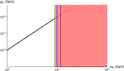
Fig. 4.3: The allowed parameter space for $\psi_{\ast}$, with $\alpha\!=\!1$, $\Gamma_{\varphi}\!\ll\!H_{TI}$ and the parameter values of LABEL:Table:_Free_Parameter_Values_(alpha=1_and_Gamma_{varphi}<<H_{TI}). The constraints on $m_{0}$ that are shown are the following: Green: LABEL:Eq.:_m_{0}_Constraint_f   Blue: LABEL:Eq.:_m_{0}_Constraint_h   Purple: LABEL:Eq.:_m_{0}_Constraint_v_(Gamma_{varphi}_<<_H_{TI})

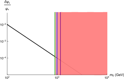
Fig. 4.4: The allowed parameter space for $\frac{\delta\psi_{\ast}}{\psi_{\ast}}$, with $\alpha\!=\!1$, $\Gamma_{\varphi}\!\ll\!H_{TI}$ and the parameter values of LABEL:Table:_Free_Parameter_Values_(alpha=1_and_Gamma_{varphi}<<H_{TI}). The constraints on $m_{0}$ that are shown are the following: Green: LABEL:Eq.:_m_{0}_Constraint_f   Blue: LABEL:Eq.:_m_{0}_Constraint_h   Purple: LABEL:Eq.:_m_{0}_Constraint_v_(Gamma_{varphi}_<<_H_{TI})

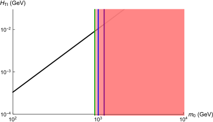
Fig. 4.5: The allowed parameter space for $H_{TI}$, with $\alpha\!=\!1$, $\Gamma_{\varphi}\!\ll\!H_{TI}$ and the parameter values of LABEL:Table:_Free_Parameter_Values_(alpha=1_and_Gamma_{varphi}<<H_{TI}). The constraints on $m_{0}$ that are shown are the following: Green: LABEL:Eq.:_m_{0}_Constraint_f   Blue: LABEL:Eq.:_m_{0}_Constraint_h   Purple: LABEL:Eq.:_m_{0}_Constraint_v_(Gamma_{varphi}_<<_H_{TI})

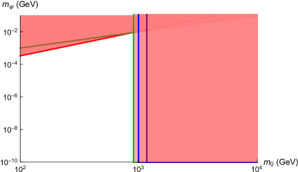
Fig. 4.6: The allowed parameter space for $m_{\psi}$, with $\alpha\!=\!1$, $\Gamma_{\varphi}\!\ll\!H_{TI}$ and the parameter values of LABEL:Table:_Free_Parameter_Values_(alpha=1_and_Gamma_{varphi}<<H_{TI}). The upper bound given by the Red line is that of LABEL:Eq.:_Psi_Mass_<<_H_{TI} and the upper bound given by the Brown line is that of Eq. 4.165. (We choose to display only down to $10^{-10}\ \mbox{GeV}$, i.e. this value is not a lower bound.) The constraints on $m_{0}$ that are shown are the following: Green: LABEL:Eq.:_m_{0}_Constraint_f   Blue: LABEL:Eq.:_m_{0}_Constraint_h   Purple: LABEL:Eq.:_m_{0}_Constraint_v_(Gamma_{varphi}_<<_H_{TI})

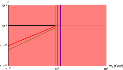
Fig. 4.7: The allowed parameter space for $h$, with $\alpha\!=\!1$, $\Gamma_{\varphi}\!\ll\!H_{TI}$ and the parameter values of LABEL:Table:_Free_Parameter_Values_(alpha=1_and_Gamma_{varphi}<<H_{TI}). The Black line is $h\!=\!10^{-9}$, the Red line is the lower bound given by Eq. 4.93 and the Brown line is the upper bound given by LABEL:Eq.:_h_Constraint_e_(Gamma_{varphi}_<<_H_{TI}). The constraints on $m_{0}$ that are shown are the following: Green: LABEL:Eq.:_m_{0}_Constraint_f   Blue: LABEL:Eq.:_m_{0}_Constraint_h   Purple: LABEL:Eq.:_m_{0}_Constraint_v_(Gamma_{varphi}_<<_H_{TI})

Values of other quantities in the model for a mass value of $m_{0}\!\sim\!10^{3}\ \mbox{GeV}$ and the parameter values of LABEL:Table:_Free_Parameter_Values_(alpha=1_and_Gamma_{varphi}<<H_{TI}) are shown in LABEL:Table:_Quantity_Values_for_m_{0}sim10^{3}_(alpha=1_and_Gamma_{varphi}<<H_{TI}). In this table we include the tensor fraction, which for a value of $H_{\ast}\!\sim\!10^{8}\ \mbox{GeV}$ yields the negligible value $r\!\sim\!10^{-13}$.

Quantity	Order of Magnitude Value
$\psi_{\ast}$	$10^{12}\ \mbox{GeV}$
$\frac{\delta\psi_{\ast}}{\psi_{\ast}}$	$10^{-4}$
$H_{TI}$	$10^{-2}\ \mbox{GeV}$
$\left\langle\phi\right\rangle$	$10^{13}\ \mbox{GeV}$
$V_{0}^{\frac{1}{4}}$	$10^{8}\ \mbox{GeV}$
$T_{1}$	$10^{7}\ \mbox{GeV}$
$T_{2}$	$10^{3}\ \mbox{GeV}$
$\Gamma$	$10^{2}\ \mbox{GeV}$
$r$	$10^{-13}$

Table 4.3: Values of quantities in the model for $\alpha\!=\!1$, $\Gamma_{\varphi}\!\ll\!H_{\textrm{TI}}$, $m_{0}\!\sim\!10^{3}\ \mbox{GeV}$ and the parameter values of LABEL:Table:_Free_Parameter_Values_(alpha=1_and_Gamma_{varphi}<<H_{TI}).

LABEL:Figure:_f_{NL} and LABEL:Figure:_g_{NL} show the prediction of the model for the non-Gaussianity parameters $f_{\textrm{NL}}$ and $g_{\textrm{NL}}$ respectively, with $h$ and $H_{\ast}$ values from LABEL:Table:_Free_Parameter_Values_(alpha=1_and_Gamma_{varphi}<<H_{TI}), together with the central value and range for the parameters as obtained by the Planck spacecraft [55]. From looking at LABEL:Figure:_g_{NL}, it may initially seem as if our predicted value for $g_{\textrm{NL}}$ for a thermal waterfall field mass value of $m_{0}\!\sim\!10^{3}\ \mbox{GeV}$ is ruled-out. However, as we are working within an order of magnitude for each value, we can see that our predicted value, i.e. the Black curve, is allowed within an order of magnitude below $m_{0}\!\sim\!10^{3}\ \mbox{GeV}$. The values of $f_{\textrm{NL}}$ and $g_{\textrm{NL}}$ for a thermal waterfall field mass of $m_{0}\!\sim\!10^{3}\ \mbox{GeV}$ are shown in LABEL:Table:_Non-Gaussianity_Parameters_for_m_{0}sim10^{3}_(alpha=1_and_Gamma_{varphi}<<H_{TI}), with them both being within current observational bounds [55].

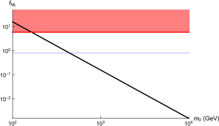
Fig. 4.8: Prediction of the model for the non-Gaussianity parameter $f_{\textrm{NL}}$, with $\alpha\!=\!1$, $\Gamma_{\varphi}\!\ll\!H_{TI}$ and $h$ and $H_{\ast}$ values from LABEL:Table:_Free_Parameter_Values_(alpha=1_and_Gamma_{varphi}<<H_{TI}). (A plot of LABEL:Eq.:_f_{NL}_-_End_of_Inflation, with $\psi\!=\!\psi_{\ast}$.) The Blue and Red lines are the central value and upper bound of $f_{\textrm{NL}}$ respectively as obtained by the Planck spacecraft [55], with the lower bound being outside the displayed range of $f_{\textrm{NL}}$.

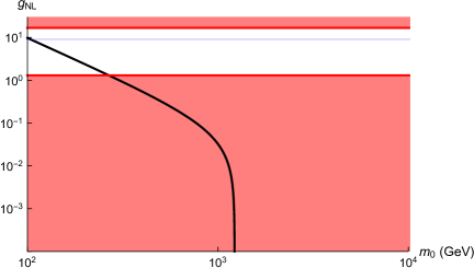
Fig. 4.9: Prediction of the model for the non-Gaussianity parameter $g_{\textrm{NL}}$, with $\alpha\!=\!1$, $\Gamma_{\varphi}\!\ll\!H_{TI}$ and $h$ and $H_{\ast}$ values from LABEL:Table:_Free_Parameter_Values_(alpha=1_and_Gamma_{varphi}<<H_{TI}). (A plot of LABEL:Eq.:_g_{NL}_-_End_of_Inflation, with $\psi\!=\!\psi_{\ast}$.) The Blue and Red lines are the central value and lower/upper bounds of $g_{\textrm{NL}}$ respectively as obtained by the Planck spacecraft [55].

Parameter	Order of Magnitude Value
$f_{\textrm{NL}}$	$10^{-1}$
$g_{\textrm{NL}}$	$10^{-2}$

Table 4.4: Prediction for non-Gaussianity parameters of the model, with $\alpha\!=\!1$, $\Gamma_{\varphi}\!\ll\!H_{\textrm{TI}}$, $m_{0}\!\sim\!10^{3}\ \mbox{GeV}$ and $h$ and $H_{\ast}$ values from LABEL:Table:_Free_Parameter_Values_(alpha=1_and_Gamma_{varphi}<<H_{TI}).

$n_{s}$ and $n_{s}^{\prime}$: Chaotic Inflation
We provide results for the spectral index and its running when the period of primordial inflation is that of slow-roll Chaotic Inflation, with the potential

$$V(\varphi)=\frac{1}{2}m_{\varphi}^{2}\varphi^{2}$$ (4.174)

From LABEL:Subsection:_Spectral_Index_---_n_{s}_and_n_{s}^{'}, the spectral index $n_{s}$ is given by

$$n_{s}\simeq 1-2\epsilon+2\eta_{\psi\psi}$$ (4.175)

with $\epsilon$ being given by Eq. 4.22 and $\eta_{\psi\psi}$ being given by LABEL:Eq.:_eta_{psi_psi}_Definition and where both are to be evaluated at the point where cosmological scales exit the horizon during primordial inflation. The potential of Eq. 4.174 gives

$$\epsilon=\frac{2M_{P}^{2}}{\varphi_{\ast}^{2}}$$ (4.176)

We obtain an expression for $\varphi_{\ast}$ in terms of $N_{\ast}$ by using the equation

$$N_{\ast}\approx\frac{1}{M_{P}^{2}}\int_{\varphi_{end}}^{\varphi_{\ast}}\frac{V(\varphi)}{V^{\prime}(\varphi)}\,\mathrm{d}\varphi$$ (4.177)

We define the end of primordial inflation to be when $\epsilon\!=\!1$. This gives

$$\varphi_{end}=\sqrt{2}M_{P}$$ (4.178)

Therefore we have

$$N_{\ast} \approx\frac{1}{M_{P}^{2}}\int_{\sqrt{2}M_{P}}^{\varphi_{\ast}}\frac{V(\varphi)}{V^{\prime}(\varphi)}\,\mathrm{d}\varphi$$ (4.179)

$$\approx\frac{1}{2M_{P}^{2}}\int_{\sqrt{2}M_{P}}^{\varphi_{\ast}}\varphi\,\mathrm{d}\varphi$$ (4.180)

$$\varphi_{\ast} \approx\sqrt{4N_{\ast}+2}\,M_{P}$$ (4.181)

Substituting LABEL:Eq.:_varphi_{*} into LABEL:Eq.:_epsilon_-_varphi_{*} gives

$$\epsilon\approx\frac{1}{2N_{\ast}+1}$$ (4.182)

We also need to calculate $\eta_{\psi\psi}$. Using our potential, Eq. 4.2, we obtain $V_{\psi\psi}$ at the time cosmological scales exit the horizon as

$$V_{\psi\psi}|_{\ast}=m_{\psi}^{2}+\left(4\alpha^{2}-2\alpha\right)h^{2}\phi_{\ast}^{2}\left(\frac{\psi_{\ast}}{M_{P}}\right)^{2\alpha-2}$$ (4.183)

Therefore we obtain $\eta_{\psi\psi}$ as

$$\eta_{\psi\psi}=\frac{1}{3H_{\ast}^{2}}\left[m_{\psi}^{2}+\left(4\alpha^{2}-2\alpha\right)h^{2}\phi_{\ast}^{2}\left(\frac{\psi_{\ast}}{M_{P}}\right)^{2\alpha-2}\right]$$ (4.184)

Our final result for the spectral index is therefore

$$n_{s}\approx 1-\frac{2}{2N_{\ast}+1}+\frac{2}{3H_{\ast}^{2}}\left[m_{\psi}^{2}+\left(4\alpha^{2}-2\alpha\right)h^{2}\phi_{\ast}^{2}\left(\frac{\psi_{\ast}}{M_{P}}\right)^{2\alpha-2}\right]$$ (4.185)

From LABEL:Subsection:_Spectral_Index_---_n_{s}_and_n_{s}^{'}, the running of the spectral index $n_{s}^{\prime}$ is given by

$$n_{s}^{\prime}\simeq-8\epsilon^{2}+4\epsilon\eta+4\epsilon\eta_{\psi\psi}$$ (4.186)

with $\eta$ being given by Eq. 4.29, which is to be evaluated at the point where cosmological scales exit the horizon during primordial inflation. The potential of Eq. 4.174 gives

$$\eta=\frac{2M_{P}^{2}}{\varphi_{\ast}^{2}}$$ (4.187)

which is identical to the value of $\epsilon$, LABEL:Eq.:_epsilon_-_varphi_{*}. Substituting LABEL:Eq.:_varphi_{*} into LABEL:Eq.:_eta_-_varphi_{*} gives

$$\eta\approx\frac{1}{2N_{\ast}+1}$$ (4.188)

Our final result for the running of the spectral index is therefore

$$n_{s}^{\prime}\approx-\frac{4}{\left(2N_{\ast}+1\right)^{2}}+\frac{4}{\left(6N_{\ast}+3\right)H_{\ast}^{2}}\left[m_{\psi}^{2}+\left(4\alpha^{2}-2\alpha\right)h^{2}\phi_{\ast}^{2}\left(\frac{\psi_{\ast}}{M_{P}}\right)^{2\alpha-2}\right]$$ (4.189)

In order to obtain $n_{s}$ and $n_{s}^{\prime}$, we first need to obtain $N_{\ast}$. The prediction of the model for $N_{\textrm{TI}}$ and $N_{\ast}$ are shown in LABEL:Figure:_N_{TI} and LABEL:Figure:_N_{*} respectively, with $n$, $g$, $H_{\ast}$, $\Gamma_{\varphi}$ and $\lambda$ values from LABEL:Table:_Free_Parameter_Values_(alpha=1_and_Gamma_{varphi}<<H_{TI}). The kink that is visible in the plot of $N_{\ast}$ at around $m_{0}\!\approx\!10^{9}\ \mbox{GeV}$ is a result of the fact that for $m_{0}$ values larger than this, we do not have any period of thermal inflation, as can be seen in the plot of $N_{\textrm{TI}}$. The values of $N_{\textrm{TI}}$ and $N_{\ast}$ for a thermal waterfall field mass of $m_{0}\!\sim\!10^{3}\ \mbox{GeV}$ are shown in LABEL:Table:_N_{TI}_and_N_{*}_for_m_{0}sim10^{3}_(Gamma_{varphi}<<H_{TI}).

Fig. 4.10: Prediction of the model for $N_{\textrm{TI}}$, with $\Gamma_{\varphi}\!\ll\!H_{TI}$ and $n$, $g$, $\Gamma_{\varphi}$ and $\lambda$ values from LABEL:Table:_Free_Parameter_Values_(alpha=1_and_Gamma_{varphi}<<H_{TI}). (A plot of LABEL:Eq.:_N_(Gamma_{varphi}_<<_H_{TI}), with $m\!=\!m_{0}$.)

Fig. 4.11: Prediction of the model for $N_{\ast}$, with $\Gamma_{\varphi}\!\ll\!H_{TI}$ and $n$, $g$, $H_{\ast}$, $\Gamma_{\varphi}$ and $\lambda$ values from LABEL:Table:_Free_Parameter_Values_(alpha=1_and_Gamma_{varphi}<<H_{TI}). (A plot of LABEL:Eq.:_N_{*}_(Gamma_{varphi}_<<_H_{TI}), with $m\!=\!m_{0}$ and $\Gamma\!=\!g^{2}m_{0}$.)

Parameter	Value
$N_{\textrm{TI}}$	$\approx\!24$
$N_{\ast}$	$\approx\!28$

Table 4.5: Prediction for $N_{\textrm{TI}}$ and $N_{\ast}$ of the model, with $\Gamma_{\varphi}\!\ll\!H_{\textrm{TI}}$, $m_{0}\!\sim\!10^{3}\ \mbox{GeV}$ and $n$, $g$, $H_{\ast}$, $\Gamma_{\varphi}$ and $\lambda$ values from LABEL:Table:_Free_Parameter_Values_(alpha=1_and_Gamma_{varphi}<<H_{TI}).

The prediction of the model for $n_{s}$ and $n_{s}^{\prime}$ for each $\phi_{\ast}$ case and for a spectator field mass at the upper bound of $m_{\psi}\!=\!10^{-2}\ \mbox{GeV}$ are shown in LABEL:Figure:_n_{s}_for_phi_{*}_Case_A, LABEL:Figure:_n_{s}'_for_phi_{*}_Case_A, LABEL:Figure:_n_{s}_for_phi_{*}_Case_B, LABEL:Figure:_n_{s}'_for_phi_{*}_Case_B, LABEL:Figure:_n_{s}_for_phi_{*}_Case_C and LABEL:Figure:_n_{s}'_for_phi_{*}_Case_C, with the parameter values of LABEL:Table:_Free_Parameter_Values_(alpha=1_and_Gamma_{varphi}<<H_{TI}). The predicted values of $n_{s}$ and $n_{s}^{\prime}$ of the model for a thermal waterfall field mass of $m_{0}\!\sim\!10^{3}\ \mbox{GeV}$ for all three $\phi_{\ast}$ Cases are the same to within at least four significant figures. They are also both insensitive to the value of $m_{\psi}$ within its allowed range. $n_{s}$ and $n_{s}^{\prime}$ are shown in LABEL:Table:_n_{s}_and_n_{s}'_for_m_{0}sim10^{3}_(alpha=1_and_Gamma_{varphi}<<H_{TI}), with them both being within current observational bounds [40].

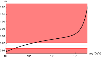
Fig. 4.12: Prediction of the model for $n_{s}$ for $\phi_{\ast}$ Case A with primordial inflation being Chaotic Inflation, with $\alpha\!=\!1$, $\Gamma_{\varphi}\!\ll\!H_{TI}$, $m_{\psi}\!=\!10^{-2}\ \mbox{GeV}$ and the parameter values from LABEL:Table:_Free_Parameter_Values_(alpha=1_and_Gamma_{varphi}<<H_{TI}). (A plot of LABEL:Eq.:_n_{s}, with $\phi_{\ast}\!=\!\left\langle\phi\right\rangle$, $m\!=\!m_{0}$ and $\Gamma\!=\!g^{2}m_{0}$.) The Blue and Red lines are the central value and lower/upper bounds of $n_{s}$ respectively as obtained by the Planck spacecraft [40].

Fig. 4.13: Prediction of the model for $n_{s}^{\prime}$ for $\phi_{\ast}$ Case A with primordial inflation being Chaotic Inflation, with $\alpha\!=\!1$, $\Gamma_{\varphi}\!\ll\!H_{TI}$, $m_{\psi}\!=\!10^{-2}\ \mbox{GeV}$ and the parameter values from LABEL:Table:_Free_Parameter_Values_(alpha=1_and_Gamma_{varphi}<<H_{TI}). (A plot of LABEL:Eq.:_n_{s}', with $\phi_{\ast}\!=\!\left\langle\phi\right\rangle$, $m\!=\!m_{0}$ and $\Gamma\!=\!g^{2}m_{0}$.) The Blue line is the central value of $n_{s}^{\prime}$ as obtained by the Planck spacecraft [40], with the lower and upper bounds being outside the displayed range of $n_{s}^{\prime}$.

Fig. 4.14: Prediction of the model for $n_{s}$ for $\phi_{\ast}$ Case B with primordial inflation being Chaotic Inflation, with $\alpha\!=\!1$, $\Gamma_{\varphi}\!\ll\!H_{TI}$, $m_{\psi}\!=\!10^{-2}\ \mbox{GeV}$ and the parameter values from LABEL:Table:_Free_Parameter_Values_(alpha=1_and_Gamma_{varphi}<<H_{TI}). (A plot of LABEL:Eq.:_n_{s}, with $\phi_{\ast}\!=\!\phi_{\textrm{BD}}$, $m\!=\!m_{0}$ and $\Gamma\!=\!g^{2}m_{0}$.) The Blue and Red lines are the central value and lower/upper bounds of $n_{s}$ respectively as obtained by the Planck spacecraft [40].

Fig. 4.15: Prediction of the model for $n_{s}^{\prime}$ for $\phi_{\ast}$ Case B with primordial inflation being Chaotic Inflation, with $\alpha\!=\!1$, $\Gamma_{\varphi}\!\ll\!H_{TI}$, $m_{\psi}\!=\!10^{-2}\ \mbox{GeV}$ and the parameter values from LABEL:Table:_Free_Parameter_Values_(alpha=1_and_Gamma_{varphi}<<H_{TI}). (A plot of LABEL:Eq.:_n_{s}', with $\phi_{\ast}\!=\!\phi_{\textrm{BD}}$, $m\!=\!m_{0}$ and $\Gamma\!=\!g^{2}m_{0}$.) The Blue line is the central value of $n_{s}^{\prime}$ as obtained by the Planck spacecraft [40], with the lower and upper bounds being outside the displayed range of $n_{s}^{\prime}$.

Fig. 4.16: Prediction of the model for $n_{s}$ for $\phi_{\ast}$ Case C with primordial inflation being Chaotic Inflation, with $\alpha\!=\!1$, $\Gamma_{\varphi}\!\ll\!H_{TI}$, $m_{\psi}\!=\!10^{-2}\ \mbox{GeV}$ and the parameter values from LABEL:Table:_Free_Parameter_Values_(alpha=1_and_Gamma_{varphi}<<H_{TI}). (A plot of LABEL:Eq.:_n_{s}, with $\phi_{\ast}\!=\!0$, $m\!=\!m_{0}$ and $\Gamma\!=\!g^{2}m_{0}$.) The Blue and Red lines are the central value and lower/upper bounds of $n_{s}$ respectively as obtained by the Planck spacecraft [40].

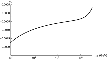
Fig. 4.17: Prediction of the model for $n_{s}^{\prime}$ for $\phi_{\ast}$ Case C with primordial inflation being Chaotic Inflation, with $\alpha\!=\!1$, $\Gamma_{\varphi}\!\ll\!H_{TI}$, $m_{\psi}\!=\!10^{-2}\ \mbox{GeV}$ and the parameter values from LABEL:Table:_Free_Parameter_Values_(alpha=1_and_Gamma_{varphi}<<H_{TI}). (A plot of LABEL:Eq.:_n_{s}', with $\phi_{\ast}\!=\!0$, $m\!=\!m_{0}$ and $\Gamma\!=\!g^{2}m_{0}$.) The Blue line is the central value of $n_{s}^{\prime}$ as obtained by the Planck spacecraft [40], with the lower and upper bounds being outside the displayed range of $n_{s}^{\prime}$.

Quantity	Value
$n_{s}$	$\approx\!0.9645$
$n_{s}^{\prime}$	$\approx\!-0.001259$

Table 4.6: Prediction for $n_{s}$ and $n_{s}^{\prime}$ of the model with primordial inflation being Chaotic Inflation, with $\alpha\!=\!1$, $\Gamma_{\varphi}\!\ll\!H_{\textrm{TI}}$, $m_{\psi}\!=\!10^{-2}\ \mbox{GeV}$, $m_{0}\!\sim\!10^{3}\ \mbox{GeV}$ and the parameter values from LABEL:Table:_Free_Parameter_Values_(alpha=1_and_Gamma_{varphi}<<H_{TI}).

4.4.4.2 The Case $\alpha\neq 1$

The present value of the effective mass of $\psi$ is

$$m_{\psi,\textrm{now}}^{2} =\left(4\alpha^{2}-2\alpha\right)h^{2}\left(\frac{\left\langle\psi\right\rangle}{M_{P}}\right)^{2\alpha-2}\left\langle\phi\right\rangle^{2}+m_{\psi}^{2}$$ (4.190)

$$m_{\psi,\textrm{now}} =m_{\psi}$$ (4.191)

the second line coming from the fact that $\left\langle\psi\right\rangle\!=\!0$ today. Therefore, from LABEL:Eq.:_m_{psi and LABEL:now}_gtrsim_1_TeV we have

$$m_{\psi}\gtrsim 1\ \mbox{TeV}$$ (4.192)

In order for this and Eq. 4.165 to both be satisfied, we require the lower bound in LABEL:Eq.:_m_{psi}_gtrsim_1_TeV to be much smaller than the upper bound in Eq. 4.165. This gives

$$m_{0}\gg 10^{8}\ \mbox{GeV}$$ (4.193)

We now require the lower bound here to be much smaller than the upper bound in LABEL:Eq.:_m_{0}_Constraint_f. This gives

$$\lambda\gg(2n+4)!\ \frac{10^{10n+26}\ \mbox{GeV${}^{2}$}}{M_{P}^{2}}$$ (4.194)

where we have explicitly factored out the $\frac{1}{(2n+4)!}$ term from our definition of $\lambda$. Given that $n\!\geq\!1$, this constraint is in conflict with the requirement that $\lambda\!\lesssim\!1$. Therefore, for $\alpha\!\neq\!1$, we find that the “end of inflation” mechanism cannot produce the dominant contribution to the observed primordial curvature perturbation within this Thermal Inflation model as it currently stands.

4.5 Modulated Decay Rate

Now we investigate the modulated decay scenario to see if it can produce the dominant contribution to the primordial curvature perturbation $\zeta$. As in Section 4.4, we aim to obtain a number of constraints on the model parameters and the initial conditions for the fields. Considering these constraints, we intend to determine the available parameter space (if any). In this parameter space we will calculate distinct observational signatures (such as non-Gaussianity) that may test this scenario in the near future.
From Section 4.3.1, the decay rate of the $\phi$ field is given by

$$\Gamma\sim g^{2}m$$ (4.195)

The primordial curvature perturbation that is produced by a varying decay rate [24] is given to first order by

$$\zeta=\delta N=-\frac{1}{6}\frac{\delta\Gamma}{\Gamma}$$ (4.196)

Differentiating $\Gamma\!\sim\!g^{2}m$ with respect to $m$ gives

$$\delta\Gamma\sim g^{2}\delta m$$ (4.197)

Therefore we obtain the primordial curvature perturbation as

$$\zeta=\delta N\sim-\frac{\delta m}{m}$$ (4.198)

This is of the same order of magnitude as the primordial curvature perturbation that is produced by the “end of inflation” mechanism, LABEL:Eq.:_Zeta_(m)_(Gamma_{varphi}_gtrsim_H_{TI}) and LABEL:Eq.:_Zeta_(m)_(Gamma_{varphi}_<<_H_{TI}).

4.5.1 Non-Gaussianity

As with the “end of inflation” mechanism scenario, we will consider what is termed local non-Gaussianity, which for the bispectrum corresponds to the “squeezed” configuration of the momenta triangle, in that the magnitude of one of the momentum vectors is much smaller than the other two, which are of similar magnitude to each other, e.g. $k_{3}\!\ll\!k_{1},k_{2}$ and $k_{1}\!\approx\!k_{2}$. Within the framework of the $\delta N$ formalism, the non-Gaussianity parameter $f_{\textrm{NL}}$ is obtained as [1]

$$f_{\textrm{NL}}=5\left(\frac{\Gamma\Gamma^{\prime\prime}}{\Gamma^{\prime^{2}}}-1\right)$$ (4.199)

where the prime denotes the derivative with respect to $\psi$. By substituting $\Gamma$ from Eq. 4.195 into LABEL:Eq.:_f_{NL}_Expression_-_Modulated_Decay_Rate we obtain

$$f_{\textrm{NL}}\sim 5\left(\frac{mm^{\prime\prime}}{m^{\prime^{2}}}-1\right)$$ (4.200)

Then, from our mass definition $m$, Eq. 4.3, we obtain

$$f_{\textrm{NL}}\sim-5\left[1+\frac{2\alpha-1}{\alpha}\left(\frac{m_{0}^{2}M_{P}^{2\alpha-2}}{2h^{2}\psi_{\ast}^{2\alpha}}-1\right)\right]$$ (4.201)

4.5.2 Constraining the Free Parameters

Regarding the constraints that appear in Section 4.4.3, all are relevant to this modulated decay scenario except for those that appear in Section 4.4.3.10, as we do not require that the transition from thermal inflation to thermal waterfall field oscillation be sufficiently fast here, as well as those appearing in Section 4.4.3.11, as the spectator field will not be oscillating in this scenario (see Section 4.5.2.2).

4.5.2.1 Time for $\phi$ Decay

After the end of thermal inflation, we require there to exist an amount of time, i.e. an amount of Universe expansion, prior to the decay of the $\phi$ field. This is so that the modulated decay rate mechanism can have an effect. If the $\phi$ field decayed immediately after the end of thermal inflation, the decay rate would not be effectively modulated. Therefore, we require

$$H_{TI}>\Gamma$$ (4.202)

Substituting LABEL:Eq.:_H_{TI} and 4.195 into here gives

$$m_{0}>\sqrt{\lambda}\ g^{2n+2}M_{P}$$ (4.203)

4.5.2.2 Light $\psi$

For the “end of inflation” mechanism scenario, we required the effective mass of $\psi$ to be light all the way up until the end of thermal inflation. However, in this modulated decay rate scenario, we require the effective mass to be light for longer, all the way up until $\phi$ decays, in order that $\psi$ does not start oscillating, so that the perturbations in $\psi$ remain at decay time and thus have the effect of perturbing the decay rate. Therefore we require

$$|m_{\psi,\textrm{eff}}|\ll H$$ (4.204)

The $\phi$ field decays when $H$ falls to $\sim\!\Gamma$. Therefore we require

$$|m_{\psi,\textrm{eff}}|\ll\Gamma$$ (4.205)

We have

$$m_{\psi,\textrm{eff}}^{2}=m_{\psi}^{2}+\left(4\alpha^{2}-2\alpha\right)h^{2}\phi^{2}\left(\frac{\psi}{M_{P}}\right)^{2\alpha-2}$$ (4.206)

Therefore we require

$$m_{\psi}\ll\Gamma$$ (4.207)

and

$$h\overline{\phi}\left(\frac{\psi_{\ast}}{M_{P}}\right)^{\alpha-1} \ll\Gamma$$ (4.208)

$$h\left\langle\phi\right\rangle\left(\frac{\psi_{\ast}}{M_{P}}\right)^{\alpha-1} \ll\Gamma$$ (4.209)

Substituting $\left\langle\phi\right\rangle$, $\psi_{\ast}$ and $\Gamma$, Eqs. 4.7, LABEL:Eq.:_Psi_{*} and 4.195 respectively, into Eq. 4.209 gives the constraint

$$h\ll\left(g^{2}m_{0}M_{P}^{\alpha-1}\right)^{2\alpha-1}\left(\frac{\sqrt{\left(2n+4\right)\lambda}}{m_{0}M_{P}^{n}}\right)^{\frac{2\alpha-1}{n+1}}\left(\frac{100\sqrt{H_{\ast}}}{m_{0}M_{P}^{\alpha-1}}\right)^{2\alpha-2}$$ (4.210)

4.5.2.3 Energy Density of the Spectator Field

We require the energy density of $\psi$ to be subdominant after thermal inflation up until it decays, in order that it does not cause any inflation by itself. The energy density of $\psi$ after thermal inflation is

$$\rho_{\psi} =h^{2}\frac{\psi_{\ast}^{2\alpha}}{M_{P}^{2\alpha-2}}\overline{\phi}^{2}+\frac{1}{2}m_{\psi}^{2}\psi_{\ast}^{2}$$ (4.211)

$$\sim h^{2}\frac{\psi_{\ast}^{2\alpha}}{M_{P}^{2\alpha-2}}\left\langle\phi\right\rangle^{2}+\frac{1}{2}m_{\psi}^{2}\psi_{\ast}^{2}$$ (4.212)

For simplicity, we assume that $\psi$ decays around the same time as $\phi$, i.e. that $H$ does not change much between the time when $\phi$ decays and the time when $\psi$ decays. Therefore, the energy density of the Universe at the time when $\psi$ decays is $\sim\!M_{P}^{2}\Gamma^{2}$. We therefore require

$$\rho_{\psi} \ll M_{P}^{2}\Gamma^{2}$$ (4.213)

$$h^{2}\frac{\psi_{\ast}^{2\alpha}}{M_{P}^{2\alpha-2}}\left\langle\phi\right\rangle^{2}+\frac{1}{2}m_{\psi}^{2}\psi_{\ast}^{2} \ll M_{P}^{2}\Gamma^{2}$$ (4.214)

Therefore we require

$$m_{\psi}\ll\frac{M_{P}\Gamma}{\psi_{\ast}}$$ (4.215)

and

$$h\left\langle\phi\right\rangle\psi_{\ast}^{\alpha}\ll M_{P}^{\alpha}\Gamma$$ (4.216)

These two constraints are identical to Eqs. 4.171 and 4.172 that appear in Section 4.4.3.11. This is easy to understand, in that the only difference between the derivation of the two constraints in Section 4.4.3.11 and those that appear here, is that, in the latter, we start with $\psi$ taking its frozen value $\psi_{\ast}$, whereas in the former, we start with $\psi$ taking its average oscillation value. However, the average oscillation value is just $\psi_{\ast}$. Substituting $\left\langle\phi\right\rangle$, $\psi_{\ast}$ and $\Gamma$, Eqs. 4.7, LABEL:Eq.:_Psi_{*} and 4.195 respectively, into Eq. 4.216 gives the constraint

$$h\gg\frac{1}{\left(g^{2}m_{0}\right)^{2\alpha-1}}\left(\frac{m_{0}M_{P}^{n}}{\sqrt{\left(2n+4\right)\lambda}}\right)^{\frac{2\alpha-1}{n+1}}\left(\frac{m_{0}}{100\sqrt{H_{\ast}M_{P}}}\right)^{2\alpha}$$ (4.217)

which is identical to Eq. 4.173.

4.5.3 Results

In order for Eqs. 4.210 and 4.217 to both be satisfied, we require the upper bound in Eq. 4.210 to be much larger than the lower bound in Eq. 4.217. This gives

$$m_{0}\ll\frac{\sqrt{(2n+4)\lambda}\left(100g^{2}\sqrt{H_{\ast}}\right)^{n+1}}{\sqrt{M_{P}}^{n-1}}$$ (4.218)

We now require this upper bound to be much larger than the lower bound in LABEL:Eq.:_m_{0}_Constraint_y. This gives

$$H_{\ast}\gg\frac{M_{P}}{10^{4}(2n+4)^{\frac{1}{n+1}}}$$ (4.219)

We now require this lower bound to be much smaller than the upper bound in LABEL:Eq.:_H_{*}_Constraint_a. This gives

$$(2n+4)^{\frac{1}{n+1}}\gg\frac{M_{P}}{10^{14}\ \mbox{GeV}}$$ (4.220)

For all values of $n$, this constraint is grossly violated. Therefore, we find that this modulated decay rate scenario cannot produce the dominant contribution to the observed primordial curvature perturbation within this Thermal Inflation model as it currently stands.

Chapter 5 Summary and Conclusions

The research activity and success that has occurred within the field of Cosmology over the last several decades, both observationally and theoretically/computationally, is vast. We have reached a point in which the amount of data being obtained observationally, as well as its precision, is of a sufficient level to strongly guide the direction that theoretical topics within Cosmology should take. This era of “Precision Cosmology” is, for example, having an ever-greater input into the topic of Inflation. It has the power to rule-out with high confidence certain models of Inflation, whilst giving further (strong) support to others.
The momentum that Cosmology research is experiencing at the moment is not just down to the field of Cosmology however. Several other fields are providing significant input into Cosmology, the main one being, at least for our work, particle physics. The topics of QFT and, in general, the Standard Model of particle physics play key roles in the development of modern Particle Cosmology.
This thesis explores one such contribution to the current state of Particle Cosmology. We have developed a model of Thermal Inflation in which a thermal waterfall scalar field, $\phi$, is coupled to a light spectator scalar field, $\psi$. If this spectator field remains light from the time of primordial inflation up until the time when the thermal waterfall field decays, then a contribution to the primordial curvature perturbation $\zeta$ will be generated by two mechanisms: “end of inflation” and modulated decay. The motivation for the creation of this new model was to determine whether it can produce the dominant contribution to the primordial curvature perturbation and then to scrutinise its predictions for various quantities that can be observationally (and theoretically) tested.
Our model explores two different cases for the decay of the inflaton $\varphi$: Inflaton decay is complete before the start of thermal inflation and inflaton decay occurs after the end of thermal inflation. We have also explored several different cases for the initial value of $\phi$ during primordial inflation, which we label $\phi_{\ast}$ Case A, B and C. With regard to the decay of the thermal waterfall field $\phi$, we have only considered the case that the decay is via direct interactions with the particles in the thermal bath that exist due to the (partial) reheating of the inflaton $\varphi$. Regarding the decay of the spectator field, we assume that this field, $\psi$, decays around the same time as the thermal waterfall field $\phi$.
We have used the $\delta N$ formalism to study the perturbations that are generated from both the “end of inflation” and modulated decay mechanisms within this model. We find that $\zeta$ is of the same magnitude to first order for both cases.
We have constrained the two mechanisms within the model by using a large array of constraints, coming from both observational and theoretical considerations. Some of these are commonplace constraints that appear in many inflation models, such as the requirement that the model does not spoil the high-degree of success of BBN. However, some of the constraints that we employ are rarely seen elsewhere in inflation model-building. Therefore, we believe that, in general, our model is significantly more comprehensive than most others and that some of our constraints should be applied to other inflation models.
We first discuss the results for the modulated decay scenario within our model. After considering all constraints together, we found strong tension between several constraints relating to $h$, $m_{0}$ and $H_{\ast}$, as these yield the constraint given by Eq. 4.220, which can never be satisfied. In conclusion therefore, we find that the modulated decay rate mechanism scenario within our model cannot produce the dominant contribution to the observed primordial curvature perturbation as it currently stands.
Now we discuss the results for the “end of inflation” scenario within our model. We first start with the case $\alpha\neq 1$. Similarly with the modulated decay scenario, after considering all constraints together, we found tension between several constraints, relating to $m_{\psi}$ and $m_{0}$. These combined constraints yield the constraint given by Eq. 4.194, which can never be satisfied, given that we require $\lambda\!\lesssim\!1$. In conclusion therefore, we find that the “end of inflation” mechanism scenario for $\alpha\neq 1$ within our model cannot produce the dominant contribution to the observed primordial curvature perturbation as it currently stands.
We now turn to the case $\alpha\!=\!1$. We have given results only for the case $\Gamma_{\varphi}\!\ll\!H_{\textrm{TI}}$. The reason for this is that this case yielded more liberal constraints than the case $\Gamma_{\varphi}\!\gtrsim\!H_{\textrm{TI}}$. For reasonable values of $H_{\ast}$ and $\Gamma_{\varphi}$, a value of $g\!=\!0.4$ yields a sharp prediction to within an order of magnitude for all but one of the quantities in the model, regardless of the $\phi_{\ast}$ case. The quantity $m_{\psi}$ can span many orders of magnitude when looking within the range $m_{0}\!\sim\!10^{2}\,\text{--}\,10^{3}\ \mbox{GeV}$ and we report only an upper bound of $m_{\psi}\!\sim\!10^{-4}\,\text{--}\,10^{-2}\ \mbox{GeV}$.
Regarding the tensor fraction, we obtain a prediction of $r\!\sim\!10^{-13}$ for a value of $H_{\ast}\!\sim\!10^{8}\ \mbox{GeV}$.
We also report values for the non-Gaussianity parameters $f_{\textrm{NL}}$ and $g_{\textrm{NL}}$ for local-type non-Gaussianity, i.e. for when the momenta triangle is in the squeezed configuration. We predict values of $f_{\textrm{NL}}\!\sim\!10^{-1}$ and $g_{\textrm{NL}}\!\sim\!10^{-2}$, for a value of $m_{0}\!\sim\!10^{3}\ \mbox{GeV}$, which are within current observational bounds.
In order to obtain predictions from our model for the scalar spectral index and its running, we needed to choose an inflation model for the period of primordial inflation. We chose to use a simple slow-roll Chaotic Inflation model, with the potential given by Eq. 4.174. We obtain values of $n_{s}\!\approx\!0.9645$ and $n_{s}^{\prime}\!\approx\!-0.001259$, for values of $m_{0}\!\sim\!10^{3}\ \mbox{GeV}$, $N_{\textrm{TI}}\!\approx\!24$ and $N_{\ast}\!\approx\!28$ and independent of the $\phi_{\ast}$ Case and the value of $m_{\psi}$ within its allowed range. These values for $n_{s}$ and $n_{s}^{\prime}$ are within current observational bounds.
As already mentioned, the analysis that we have performed on our model has been limited to a relatively small region of the vast parameter space. Therefore, it is possible that there exist other allowed regions, for different values of some or all of the free parameters in the model. This is a potential area for future research. In addition, as our analysis has been purely analytical, where we have analysed most quantities to within an order of magnitude, a future area of work could be to perform numerical analysis. In particular, the constraint that was imposed in order that the inflationary trajectory was 1-dimensional, in that only the $\phi$ field was involved in determining the trajectory of thermal inflation in field space, could be removed, as a numerical analysis lends itself better to such multi-dimensional inflationary trajectories than does an analytic one.
Cosmology is still experiencing a golden era at present, with ever more data and theoretical insight progressing the field and giving rise to breakthroughs. We can hope that this situation and momentum grows, with it continuing to lead us on an incredibly exciting journey further down the avenue of the most fundamental questions that humankind can ask.

Appendix A Derivation of Thermal Fluctuation of $\phi$

Our aim is to calculate the thermal fluctuation of $\phi$ that exists when the field is in thermal equilibrium with a thermal bath. This derivation has been worked through following Ref. [56]. As we are dealing with the thermal fluctuation of $\phi$ about $\phi=0$, we will simply call $\delta\phi$ by $\phi$.
The solution to the perturbation equation

$$\ddot{\phi}-\nabla^{2}\phi+V^{\prime\prime}\phi=0$$ (A.1)

is

$$\phi=\frac{1}{\sqrt{16\pi^{3}}}\int\frac{1}{\sqrt{\omega_{k}}}\left(e^{-i\omega_{k}t+i\textbf{k}\cdot\textbf{x}}a_{\textbf{k}}^{-}+e^{i\omega_{k}t-i\textbf{k}\cdot\textbf{x}}a_{\textbf{k}}^{+}\right)\,\mathrm{d^{3}}\!k$$ (A.2)

where

$$\omega_{k}=\sqrt{k^{2}+\left|m_{\phi,\textrm{eff}}^{2}\right|}$$ (A.3)

Using

$$\left\langle\hat{a}_{\textbf{k}}^{+}\hat{a}_{\textbf{k}^{\prime}}^{-}\right\rangle\equiv\frac{\left\langle n_{\textbf{k}}\left|\hat{a}_{\textbf{k}}^{+}\hat{a}_{\textbf{k}^{\prime}}^{-}\right|n_{\textbf{k}}\right\rangle}{\left\langle n_{\textbf{k}}|n_{\textbf{k}}\right\rangle}=n_{\textbf{k}}\delta\!\left(\textbf{k}-\textbf{k}^{\prime}\right)$$ (A.4)

and

$$\left\langle\hat{a}_{\textbf{k}}^{+}\hat{a}_{\textbf{k}^{\prime}}^{+}\right\rangle=\left\langle\hat{a}_{\textbf{k}}^{-}\hat{a}_{\textbf{k}^{\prime}}^{-}\right\rangle=0$$ (A.5)

where $n_{\textbf{k}}$ is the occupation number, as well as the commutation relation

$$\left[\hat{a}_{\textbf{k}}^{-},\hat{a}_{\textbf{k}^{\prime}}^{+}\right]=\delta\!\left(\textbf{k}-\textbf{k}^{\prime}\right)$$ (A.6)

we obtain the 2-point correlator as

$$\left\langle\phi^{2}\right\rangle=\frac{1}{16\pi^{3}}\iint\frac{1}{\sqrt{\omega_{k}\omega_{k^{\prime}}}}\left(e^{-i\omega_{k}t+i\textbf{k}\cdot\textbf{x}+i\omega_{k^{\prime}}t-i\textbf{k}^{\prime}\cdot\textbf{x}}\left(\delta\!\left(\textbf{k}-\textbf{k}^{\prime}\right)+\left\langle\hat{a}_{\textbf{k}^{\prime}}^{+}\hat{a}_{\textbf{k}}^{-}\right\rangle\right)\right.\\ +\left.e^{i\omega_{k}t-i\textbf{k}\cdot\textbf{x}-i\omega_{k^{\prime}}t+i\textbf{k}^{\prime}\cdot\textbf{x}}\left\langle\hat{a}_{\textbf{k}}^{+}\hat{a}_{\textbf{k}^{\prime}}^{-}\right\rangle\right)\,\mathrm{d^{3}}\!k\ \mathrm{d^{3}}\!k^{\prime}$$ (A.7)

Working through the integral, we obtain

$$\left\langle\phi^{2}\right\rangle =\frac{1}{8\pi^{3}}\int\frac{1}{\omega_{k}}\left(\frac{1}{2}+n_{\textbf{k}}\right)\,\mathrm{d^{3}}\!k$$ (A.8)

$$=\frac{1}{8\pi^{3}}\int_{0}^{\infty}\frac{k^{2}}{\omega_{k}}\left(\frac{1}{2}+n_{\textbf{k}}\right)\,\mathrm{d}k\,\int_{0}^{\pi}\mathrm{\sin}\!\left(\theta\right)\,\mathrm{d}\theta\,\int_{0}^{2\pi}\mathrm{d}\varphi$$ (A.9)

$$=\frac{1}{2\pi^{2}}\int_{0}^{\infty}\frac{k^{2}}{\omega_{k}}\left(\frac{1}{2}+n_{\textbf{k}}\right)\,\mathrm{d}k$$ (A.10)

The occupation number $n_{\textbf{k}}$ is given by the Bose-Einstein distribution

$$n_{\omega_{k}}=\frac{1}{e^{\frac{\omega_{k}}{T}}-1}$$ (A.11)

where we are neglecting the chemical potential. Substituting this into LABEL:Eq.:_<phi^2>_--_n_{k} gives

$$\left\langle\phi^{2}\right\rangle_{T}=\frac{1}{2\pi^{2}}\int_{0}^{\infty}\frac{k^{2}}{\omega_{k}\left(e^{\frac{\omega_{k}}{T}}-1\right)}\,\mathrm{d}k$$ (A.12)

The $\frac{1}{2}$ term that appears in LABEL:Eq.:_<phi^2>_--_n_{k} is not present in LABEL:Eq.:_<phi^2>_{T}_--_k as it can be removed by one of the following:

• Having $n_{\omega_{k}}\gg\frac{1}{2}$

• Subtracting the vacuum

• Performing normal ordering

LABEL:Eq.:_<phi^2>_{T}_--_k can be expressed as

$$\left\langle\phi^{2}\right\rangle_{T}=\frac{T^{2}}{4\pi^{2}}J_{-}^{\left(1\right)}\left(\frac{|m_{\phi,\textrm{eff}}|}{T},0\right)$$ (A.13)

The proof is as follows. The definition of the $J$ term is

$$J_{\mp}^{\left(\nu\right)}(\kappa,\tau)\equiv\int_{\kappa}^{\infty}\frac{\left(x^{2}-\kappa^{2}\right)^{\frac{\nu}{2}}}{e^{x-\tau}\mp 1}\,\mathrm{d}x+\int_{\kappa}^{\infty}\frac{\left(x^{2}-\kappa^{2}\right)^{\frac{\nu}{2}}}{e^{x+\tau}\mp 1}\,\mathrm{d}x$$ (A.14)

where for our derivation we define

$$\kappa\equiv\frac{|m_{\phi,\textrm{eff}}|}{T}\hskip 50.00008pt\tau\equiv\frac{\mu}{T}$$ (A.15)

where $\mu$ is the chemical potential. Therefore we obtain (with $\tau\!=\!0$ as $\mu\!=\!0$)

$$J_{-}^{\left(1\right)}\left(\frac{|m_{\phi,\textrm{eff}}|}{T},0\right)\equiv 2\int_{\frac{\left|m_{\phi,\textrm{eff}}\right|}{T}}^{\infty}\frac{\sqrt{x^{2}-\left(\frac{|m_{\phi,\textrm{eff}}|}{T}\right)^{2}}}{e^{x}-1}\,\mathrm{d}x$$ (A.16)

Substituting this into LABEL:Eq.:_<phi^{2}>_{T}_--_J gives

$$\left\langle\phi^{2}\right\rangle_{T}=\frac{T^{2}}{2\pi^{2}}\int_{\frac{\left|m_{\phi,\textrm{eff}}\right|}{T}}^{\infty}\frac{\sqrt{x^{2}-\left(\frac{|m_{\phi,\textrm{eff}}|}{T}\right)^{2}}}{e^{x}-1}\,\mathrm{d}x$$ (A.17)

Now, we can obtain LABEL:Eq.:_<phi^{2}>_{T}_--_x from LABEL:Eq.:_<phi^2>_{T}_--_k by simply changing the integration variable as

$$k\rightarrow x \equiv\frac{\omega_{k}}{T}$$ (A.18)

$$=\frac{\sqrt{k^{2}+\left|m_{\phi,\textrm{eff}}^{2}\right|}}{T}$$ (A.19)

$$\mathrm{d}x =\frac{k}{\omega_{k}T}\,\mathrm{d}k$$ (A.20)

We can make progress in trying to solve the integral of $J_{-}^{\left(1\right)}$ as follows. $J_{-}^{\left(-1\right)}$ can be written as

$$J_{-}^{\left(-1\right)}=2\sum_{n=1}^{\infty}K_{0}(n\kappa)$$ (A.21)

where $K$ is the modified Bessel function of the second kind. There exists a recurrence relation

$$\frac{\partial J_{\mp}^{\left(\nu\right)}}{\partial\kappa}=-\nu\kappa J_{\mp}^{\left(\nu-2\right)}$$ (A.22)

Therefore we have

$$J_{-}^{\left(1\right)} =-\int\kappa J_{-}^{\left(-1\right)}\,\mathrm{d}\kappa$$ (A.23)

$$=-2\int\kappa\sum_{n=1}^{\infty}K_{0}(n\kappa)\,\mathrm{d}\kappa$$ (A.24)

The summation of the modified Bessel functions can be expressed as

$$\sum_{n=1}^{\infty}K_{0}(n\kappa)=\frac{1}{2}\left[\underline{C}+\ln{\left(\frac{\kappa}{4\pi}\right)}\right]+\frac{\pi}{2\kappa}+\pi\sum_{l=1}^{\infty}\left(\frac{1}{\sqrt{\kappa^{2}+4l^{2}\pi^{2}}}-\frac{1}{2l\pi}\right)$$ (A.25)

as given in Ref. [57], where $\underline{C}$ is Euler’s constant. Therefore we obtain

$$J_{-}^{\left(1\right)}=-\int\left[\underline{C}\kappa+\kappa\ln{\left(\frac{\kappa}{4\pi}\right)}+\pi+2\pi\kappa\sum_{l=1}^{\infty}\left(\frac{1}{\sqrt{\kappa^{2}+4l^{2}\pi^{2}}}-\frac{1}{2l\pi}\right)\right]\,\mathrm{d}\kappa$$ (A.26)

In general, this integral doesn’t converge, due to the summation term. However, for $\kappa\!\ll\!1$, the summation term vanishes and the integral does converge. We adopt this case, with only a mild constraint on $g$ being introduced. From the definition of $\kappa$, Eq. A.15, $\kappa\!\ll\!1$ requires

$$T\gg|m_{\phi,\textrm{eff}}|$$ (A.27)

As we are considering the time of the end of primordial inflation, $|m_{\phi,\textrm{eff}}|\!\sim\!g\,T_{\textrm{end,inf}}$, as given by Eq. 4.99. Therefore we have

$$T_{\textrm{end,inf}} \gg gT_{\textrm{end,inf}}$$ (A.28)

$$g \ll 1$$ (A.29)

So, we now have

$$J_{-}^{\left(1\right)}\simeq-\frac{1}{2}\underline{C}\kappa^{2}+\frac{1}{4}\kappa^{2}-\frac{1}{2}\kappa^{2}\ln{\left(\frac{\kappa}{4\pi}\right)}-\pi\kappa+A$$ (A.30)

where $A$ is a constant of integration. We can obtain $A$ by equating LABEL:Eq.:_J_{-}^{1}_--_Integral_Solved with Eq. A.14 and setting $\kappa\!=\!\tau\!=\!0$. We obtain

$$A =2\int_{0}^{\infty}\frac{x}{e^{x}-1}\,\mathrm{d}x$$ (A.31)

$$=\frac{\pi^{2}}{3}$$ (A.32)

Given that $|m_{\phi,\textrm{eff}}|\!\sim\!g\,T_{\textrm{end,inf}}$, we have $\kappa\!=\!g$. Therefore LABEL:Eq.:_J_{-}^{1}_--_Integral_Solved becomes

$$J_{-}^{\left(1\right)}\simeq\frac{\pi^{2}}{3}-\pi g-\frac{1}{2}g^{2}\ln{\left(\frac{g}{4\pi}\right)}-\frac{1}{2}\underline{C}\,g^{2}+\frac{1}{4}g^{2}$$ (A.33)

For all values of $g$, i.e. $g\!\leq\!1$, we have

$$J_{-}^{\left(1\right)}\sim\frac{\pi^{2}}{3}$$ (A.34)

Substituting this into LABEL:Eq.:_<phi^{2}>_{T}_--_J gives

$$\left\langle\phi^{2}\right\rangle_{T} \sim\frac{T^{2}}{12}$$ (A.35)

$$\sqrt{\left\langle\phi^{2}\right\rangle_{T}} \sim T$$ (A.36)

Appendix B Field Theory Derivation of Elastic Scattering Cross-section between $\phi$ and a Thermal Bath

We assume the thermal bath to only consist of one scalar field, which we call $\chi$. We define the following 4-momenta: $p_{1}$ for a $\phi$ particle before the collision, $p_{2}$ for a $\chi$ particle before the collision, $p_{3}$ for a $\phi$ particle after the collision and $p_{4}$ for a $\chi$ particle after the collision. Working within the centre-of-mass frame, the 4-momenta are:

$$p_{1} =(E_{1},\textbf{p})$$ (B.1)

$$p_{2} =(p,-\textbf{p})$$ (B.2)

$$p_{3} =\left(E_{3},\textbf{p}^{\prime}\right)$$ (B.3)

$$p_{4} =\left(p^{\prime},-\textbf{p}^{\prime}\right)$$ (B.4)

The differential elastic cross-section is given by

$$\mathrm{d}\sigma=\frac{1}{|\textbf{v}_{1}-\textbf{v}_{2}|}\frac{1}{2E_{1}}\frac{1}{2p}\left|-ig^{2}\right|^{2}\frac{\mathrm{d^{3}}\textbf{p}^{\prime}}{(2\pi)^{3}2E_{3}}\frac{\mathrm{d^{3}}(-\textbf{p}^{\prime})}{(2\pi)^{3}2p^{\prime}}(2\pi)^{4}\delta^{4}(p_{1}+p_{2}-p_{3}-p_{4})$$ (B.5)

where $\textbf{v}_{1}$ and $\textbf{v}_{2}$ are the velocities of the $\phi$ and $\chi$ particles before the collision respectively, where $\textbf{v}_{2}\!=\!c$. As we are setting $c\!=\!1$, the first term in Eq. B.5 $\approx\!1$. Collecting terms together gives

$$\mathrm{d}\sigma\approx-\frac{g^{4}}{64\pi^{2}E_{1}E_{3}pp^{\prime}}\delta^{4}(p_{1}+p_{2}-p_{3}-p_{4})\mathrm{d^{3}}\textbf{p}^{\prime}\,\mathrm{d^{3}}(-\textbf{p}^{\prime})$$ (B.6)

Integrating this gives

$$\sigma \approx-\frac{g^{4}}{64\pi^{2}E_{1}E_{3}}\iint\frac{1}{pp^{\prime}}\delta^{4}(p_{1}+p_{2}-p_{3}-p_{4})\mathrm{d^{3}}\textbf{p}^{\prime}\,\mathrm{d^{3}}(-\textbf{p}^{\prime})$$ (B.7)

$$\approx-\frac{g^{4}}{64\pi^{2}E_{1}E_{3}}\int\frac{1}{pp^{\prime}}\delta(E_{1}+p-E_{3}-p^{\prime})\mathrm{d^{3}}\textbf{p}^{\prime}$$ (B.8)

$$\approx-\frac{g^{4}}{64\pi^{2}E_{1}E_{3}}\int\frac{1}{p}\delta(E_{1}+p-E_{3}-p^{\prime})p^{\prime}\mathrm{d}p^{\prime}\int\limits_{\Omega}\mathrm{d}\Omega$$ (B.9)

From the 4-momenta of $p_{1}$ and $p_{3}$, LABEL:Eq.:_p_{1} and LABEL:Eq.:_p_{3} respectively, we have

$$E_{1}=\sqrt{p^{2}+m_{\phi,\textrm{eff}}^{2}}$$ (B.10)

and

$$E_{3}=\sqrt{p^{\prime 2}+m_{\phi,\textrm{eff}}^{2}}$$ (B.11)

Substituting these equations into Eq. B.9 gives

$$\sigma\approx-\frac{g^{4}}{64\pi^{2}E_{1}E_{3}}\int\frac{1}{p}\delta\left(\sqrt{p^{2}+m_{\phi,\textrm{eff}}^{2}}+p-\sqrt{p^{\prime 2}+m_{\phi,\textrm{eff}}^{2}}-p^{\prime}\right)p^{\prime}\mathrm{d}p^{\prime}\int\limits_{\Omega}\mathrm{d}\Omega$$ (B.12)

The argument of the delta function is only $=\!0$ if $p^{\prime}\!=\!p$. Therefore we have

$$\sigma\approx-\frac{g^{4}}{64\pi^{2}E_{1}^{2}}\int\limits_{\Omega}\mathrm{d}\Omega$$ (B.13)

We have

$$E_{1}^{2}=p^{2}+m_{\phi,\textrm{eff}}^{2}$$ (B.14)

From the 4-momenta of $p_{2}$, LABEL:Eq.:_p_{2}, we know that $E_{2}\!=\!p$. In addition, given that the energy of a $\chi$ particle is $T$, we therefore have

$$E_{1}^{2}=T^{2}+m_{\phi,\textrm{eff}}^{2}$$ (B.15)

Let us consider the time of primordial inflation reheating. We have

$$m_{\phi,\textrm{eff}}\sim gT$$ (B.16)

Therefore

$$E_{1}^{2} \sim\left(1+g^{2}\right)T^{2}$$ (B.17)

$$\sim T^{2}$$ (B.18)

Substituting LABEL:Eq.:_E_{1}^{2}_(3) into Eq. B.13 gives

$$\sigma \approx-\frac{g^{4}}{64\pi^{2}T^{2}}\int\limits_{\Omega}\mathrm{d}\Omega$$ (B.19)

$$\approx-\frac{g^{4}}{16\pi T^{2}}$$ (B.20)

$$|\sigma| \approx\frac{g^{4}}{16\pi T^{2}}$$ (B.21)

Bibliography

- [1] D. H. Lyth and A. R. Liddle, The Primordial Density Perturbation: Cosmology, Inflation and the Origin of Structure. Cambridge University Press, 2009.
- [2] D. H. Lyth and D. Wands, Generating the curvature perturbation without an inflaton, Phys.Lett. B524 (2002) 5–14, arXiv:hep-ph/0110002v2 [hep-ph].
- [3] D. H. Lyth, C. Ungarelli and D. Wands, The Primordial density perturbation in the curvaton scenario, Phys.Rev. D67 (2003) 023503, arXiv:astro-ph/0208055v3 [astro-ph].
- [4] K.-Y. Choi and O. Seto, Modulated reheating by curvaton, Phys.Rev. D85 (2012) 123528, arXiv:1204.1419v1 [astro-ph.CO].
- [5] K. Dimopoulos, Can a vector field be responsible for the curvature perturbation in the Universe?, Phys.Rev. D74 (2006) 083502, arXiv:hep-ph/0607229v2 [hep-ph].
- [6] K. Dimopoulos, M. Karciauskas, D. H. Lyth and Y. Rodriguez, Statistical anisotropy of the curvature perturbation from vector field perturbations, JCAP 0905 (2009) 013, arXiv:0809.1055v5 [astro-ph].
- [7] K. Dimopoulos and M. Karciauskas, Non-minimally coupled vector curvaton, JHEP 0807 (2008) 119, arXiv:0803.3041v2 [hep-th].
- [8] M. Karciauskas, The Primordial Curvature Perturbation from Vector Fields of General non-Abelian Groups, JCAP 1201 (2012) 014, arXiv:1104.3629v2 [astro-ph.CO].
- [9] K. Dimopoulos, Statistical Anisotropy and the Vector Curvaton Paradigm, Int.J.Mod.Phys. D21 (2012) 1250023, arXiv:1107.2779v2 [hep-ph].
- [10] K. Dimopoulos, Erratum: Statistical Anisotropy and the Vector Curvaton Paradigm, Int.J.Mod.Phys. D21 (2012) 1292003, arXiv:1107.2779v2 [hep-ph].
- [11] M. Karciauskas, K. Dimopoulos and D. H. Lyth, Anisotropic non-Gaussianity from vector field perturbations, Phys.Rev. D80 (2009) 023509, arXiv:0812.0264v2 [astro-ph].
- [12] M. Karciauskas, K. Dimopoulos and D. H. Lyth, Erratum: Anisotropic non-Gaussianity from vector field perturbations, Phys.Rev. D85 (2012) 069905(E), arXiv:0812.0264v2 [astro-ph].
- [13] S. Yokoyama and J. Soda, Primordial statistical anisotropy generated at the end of inflation, JCAP 0808 (2008) 005, arXiv:0805.4265v6 [astro-ph].
- [14] K. Dimopoulos, D. Wills and I. Zavala, Statistical Anisotropy from Vector Curvaton in D-brane Inflation, arXiv:1108.4424v2 [hep-th].
- [15] N. Bartolo, E. Dimastrogiovanni, S. Matarrese and A. Riotto, Anisotropic Trispectrum of Curvature Perturbations Induced by Primordial Non-Abelian Vector Fields, JCAP 0911 (2009) 028, arXiv:0909.5621v2 [astro-ph.CO].
- [16] K. Dimopoulos, Supergravity inspired Vector Curvaton, Phys.Rev. D76 (2007) 063506, arXiv:0705.3334v1 [hep-ph].
- [17] K. Dimopoulos and M. Karciauskas, Parity Violating Statistical Anisotropy, JHEP 1206 (2012) 040, arXiv:1203.0230v3 [hep-ph].
- [18] K. Dimopoulos, G. Lazarides and J. M. Wagstaff, Eliminating the -problem in SUGRA Hybrid Inflation with Vector Backreaction, JCAP 1202 (2012) 018, arXiv:1111.1929v2 [astro-ph.CO].
- [19] H. Assadullahi, H. Firouzjahi, M. H. Namjoo and D. Wands, Modulated curvaton decay, arXiv:1301.3439v1 [hep-th].
- [20] D. Langlois and T. Takahashi, Density Perturbations from Modulated Decay of the Curvaton, arXiv:1301.3319v1 [astro-ph.CO].
- [21] S. Enomoto, K. Kohri and T. Matsuda, Modulated decay in the multi-component Universe, arXiv:1301.3787v1 [hep-ph].
- [22] K. Kohri, C.-M. Lin and T. Matsuda, Delta-N Formalism for Curvaton with Modulated Decay, arXiv:1303.2750v1 [hep-ph].
- [23] K. Dimopoulos, G. Lazarides, D. Lyth and R. Ruiz de Austri, Curvaton dynamics, Phys.Rev. D68 (2003) 123515, arXiv:hep-ph/0308015v1 [hep-ph].
- [24] G. Dvali, A. Gruzinov and M. Zaldarriaga, New mechanism for generating density perturbations from inflation, Phys.Rev. D69 (2004) 023505, arXiv:astro-ph/0303591v1 [astro-ph].
- [25] G. Dvali, A. Gruzinov and M. Zaldarriaga, Cosmological perturbations from inhomogeneous reheating, freezeout, and mass domination, Phys.Rev. D69 (2004) 083505, arXiv:astro-ph/0305548v1 [astro-ph].
- [26] M. Postma, Inhomogeneous reheating scenario with low scale inflation and/or MSSM flat directions, JCAP 0403 (2004) 006, arXiv:astro-ph/0311563v2 [astro-ph].
- [27] F. Vernizzi, Generating cosmological perturbations with mass variations, Nucl.Phys.Proc.Suppl. 148 (2005) 120–127, arXiv:astro-ph/0503175v1 [astro-ph].
- [28] F. Vernizzi, Cosmological perturbations from varying masses and couplings, Phys.Rev. D69 (2004) 083526, arXiv:astro-ph/0311167v3 [astro-ph].
- [29] M. Zaldarriaga, Non-Gaussianities in models with a varying inflaton decay rate, Phys.Rev. D69 (2004) 043508, arXiv:astro-ph/0306006v1 [astro-ph].
- [30] M. Kawasaki, T. Takahashi and S. Yokoyama, Density Fluctuations in Thermal Inflation and Non-Gaussianity, JCAP 0912 (2009) 012, arXiv:0910.3053v3 [hep-th].
- [31] D. H. Lyth, Generating the curvature perturbation at the end of inflation, JCAP 0511 (2005) 006, arXiv:astro-ph/0510443v3 [astro-ph].
- [32] M. P. Salem, On the generation of density perturbations at the end of inflation, Phys.Rev. D72 (2005) 123516, arXiv:astro-ph/0511146v5 [astro-ph].
- [33] L. Alabidi and D. H. Lyth, Curvature perturbation from symmetry breaking the end of inflation, JCAP 0608 (2006) 006, arXiv:astro-ph/0604569v3 [astro-ph].
- [34] D. H. Lyth, The hybrid inflation waterfall and the primordial curvature perturbation, JCAP 1205 (2012) 022, arXiv:1201.4312v4 [astro-ph.CO].
- [35] D. H. Lyth and A. Riotto, Generating the Curvature Perturbation at the End of Inflation in String Theory, Phys.Rev.Lett. 97 (2006) 121301, arXiv:astro-ph/0607326v1 [astro-ph].
- [36] M. Sasaki, Multi-brid inflation and non-Gaussianity, Prog.Theor.Phys. 120 (2008) 159–174, arXiv:0805.0974v3 [astro-ph].
- [37] F. Bernardeau, L. Kofman and J.-P. Uzan, Modulated fluctuations from hybrid inflation, Phys.Rev. D70 (2004) 083004, arXiv:astro-ph/0403315v1 [astro-ph].
- [38] T. Matsuda, Cosmological perturbations from an inhomogeneous phase transition, Class.Quant.Grav. 26 (2009) 145011, arXiv:0902.4283v3 [hep-ph].
- [39] L. Alabidi, K. Malik, C. T. Byrnes and K.-Y. Choi, How the curvaton scenario, modulated reheating and an inhomogeneous end of inflation are related, JCAP 1011 (2010) 037, arXiv:1002.1700v2 [astro-ph.CO].
- [40] Planck Collaboration, P. A. R. Ade et al., Planck 2015 results. XIII. Cosmological parameters, arXiv:1502.01589v2 [astro-ph.CO].
- [41] ESA: C. Carreau, The History of Structure Formation in the Universe, March, 2013. {http://sci.esa.int/science-e-media/img/68/Planck_history_of_Universe_Crop_orig.jpg}. Downloaded 01/10/2016.
- [42] ESA: Planck Collaboration, Cosmic Microwave Background seen by Planck, March, 2013. {http://sci.esa.int/science-e-media/img/61/Planck_CMB_Mollweide_wallpaper.jpg}. Downloaded 12/10/2015.
- [43] ESA: Planck Collaboration, Planck’s Power Spectrum of Temperature Fluctuations in the Cosmic Microwave Background, March, 2013. {http://sci.esa.int/science-e-media/img/63/Planck_power_spectrum_orig.jpg}. Downloaded 12/10/2015.
- [44] A. H. Guth, The Inflationary Universe: A Possible Solution to the Horizon and Flatness Problems, Phys. Rev. D23 (1981) 347–356.
- [45] T. S. Bunch and P. C. W. Davies, Quantum Field Theory in de Sitter Space: Renormalization by Point Splitting, Proc. Roy. Soc. Lond. A360 (1978) 117–134.
- [46] D. H. Lyth, K. A. Malik and M. Sasaki, A General proof of the conservation of the curvature perturbation, JCAP 0505 (2005) 004, arXiv:astro-ph/0411220v3 [astro-ph].
- [47] D. H. Lyth and E. D. Stewart, Cosmology with a TeV mass GUT Higgs, Phys.Rev.Lett. 75 (1995) 201–204, arXiv:hep-ph/9502417v1 [hep-ph].
- [48] D. H. Lyth and E. D. Stewart, Thermal inflation and the moduli problem, Phys.Rev. D53 (1996) 1784–1798, arXiv:hep-ph/9510204v2 [hep-ph].
- [49] T. Barreiro, E. J. Copeland, D. H. Lyth and T. Prokopec, Some aspects of thermal inflation: The Finite temperature potential and topological defects, Phys.Rev. D54 (1996) 1379–1392, arXiv:hep-ph/9602263v2 [hep-ph].
- [50] T. Asaka and M. Kawasaki, Cosmological moduli problem and thermal inflation models, Phys.Rev. D60 (1999) 123509, arXiv:hep-ph/9905467v1 [hep-ph].
- [51] C. T. Byrnes, M. Sasaki and D. Wands, Primordial trispectrum from inflation, Phys. Rev. D74 (2006) 123519, arXiv:astro-ph/0611075v2 [astro-ph].
- [52] M. Dine, L. Randall and S. D. Thomas, Supersymmetry breaking in the early universe, Phys. Rev. Lett. 75 (1995) 398–401, arXiv:hep-ph/9503303v2 [hep-ph].
- [53] M. Dine, L. Randall and S. D. Thomas, Baryogenesis from flat directions of the supersymmetric standard model, Nucl. Phys. B458 (1996) 291–326, arXiv:hep-ph/9507453v1 [hep-ph].
- [54] D. H. Lyth and T. Moroi, The Masses of weakly coupled scalar fields in the early universe, JHEP 05 (2004) 004, arXiv:hep-ph/0402174v2 [hep-ph].
- [55] Planck Collaboration, P. A. R. Ade et al., Planck 2015 results. XVII. Constraints on primordial non-Gaussianity, arXiv:1502.01592v2 [astro-ph.CO].
- [56] V. Mukhanov, Physical Foundations of Cosmology. Cambridge University Press, 2005.
- [57] I. Gradshteyn and I. Ryzhik, Table of Integrals, Series and Products, 5th ed. Academic Press, 1994.