Magnetooptical Properties of Rydberg Excitons - Center-of-Mass Quantization Approach

Abstract

We show how to compute the magnetooptical functions (absorption, reflection, and transmission) when Rydberg Exciton-Polaritons appear, including the effect of the coherence between the electron-hole pair and the electromagnetic field, and the polaritonic effect. Using the Real Density Matrix Approach the analytical expressions for magnetooptical functions are obtained and numerical calculations for Cu₂0 crystal are performed. The influence of the strength of applied external magnetic field on the resonance displacement of excitonic spectra is discussed. We report a good agreement with recently published experimental data.

I Introduction

The concept of excitons has been formulated more than 80 years ago by Y. Frenkel Frenkel , who predicted their existence in molecular crystals. A few years later, G. Wannier Wannier and N. de Mott Mott described these electron-hole bound states for inorganic semiconductors. In 1952 E. Gross and N. Karriiev Gross discovered such Wannier-Mott excitons experimentally in a copper oxide semiconductor. After that time excitons remain an important topic of experimental and theoretical research, since they play a dominant role in the optical properties of semiconductors (molecular crystals etc.,). The excitons have been studied in great details in various types of semiconductor nanostructures and in bulk crystals. Since there is a large number of papers, monographs, review articles devoted to excitons, we refer to only a small collection of them Knox -Agran2009 . In the past decades the main effort of the researchers was focussed on excitons in nanostructures Weisbuch -Harrison , but very recently, new attention has been drawn back to the subject of excitons in bulk crystals by an experimental observation of the so-called yellow exciton series in Cu₂O up to a large principal quantum number of n = 25 Kazimierczuk . Such excitons in copper oxide, in analogy to atomic physics, have been named Rydberg excitons. By virtue of their special properties Rydberg excitons are of fascination in solid and optical physics. These objects whose size scales as the square of the Rydberg principal quantum number n, are ideally suited for fundamental quantum interrogations, as well as detailed classical analysis. Several theoretical approaches to calculate optical properties of Rydberg excitons have been presented Hofling -Schweiner.Symmetry . Recently quantum coherence of Rydberg excitons in this system has been investigated Gruenewald which opens new avenue for their further implementation in quantum information processing.

When external constant fields (electric or/and magnetic) are applied, the Rydberg excitons, especially those with high principal number n, show effects which are not observable in exciton systems with a few number of excitonic states. This effects range from a large Stark shift, overlapping of states, creation of higher order excitons (F, H, etc) to quantum chaos and new type statistics for exciton states assmann . Although the Stark and other electrooptic effects on Rydberg excitons in Cu₂O have been measured and analized Thewes , Heck , Zielinska.PRB.2016.b , there are only few results available regarding the magnetooptic properties of Rydberg excitons assmann where the excitonic spectra of coprous oxide subjected to an external magnetic field up to 7 T has been measured and the complex splitting pattern of crossing and overlapping levels has been demonstrated.

Highly excited Rydberg excitons in Cu₂O crystal provide a well-accessible venue for combined theoretical and experimental studies of magnetic field effects on the systems. From a different perspective magnetic fields may offer a promising possibility for a controlled manipulation of Rydberg excitons, which would be otherwise difficult to trap by standard optical techniques, developed for ground states. Due to the fact that free-space Rydberg polaritons have recently drawn intense interest as tools for quantum information processing one can expected Rydberg excitons in solid may become highly required object for creating high-fidelity photonic quantum materials jia . Magnetic fields can strongly affect the Rydberg-Rydberg interactions by breaking the Zeeman degeneracy that produces Foster zeros.

In the presented paper we will focus on magnetooptical properties of Rydberg excitons in Cu₂O motivated by the results presented in assmann . As in our previous papers Zielinska.PRB , Zielinska.PRB.2016.b , we will use the method based on the Real Density Matrix Approach (RDMA). Our main purpose is to obtain the analytical expressions for the magnetooptical functions of semiconductor crystals (reflectivity, transmissivity, absorption, and bulk magnetosusceptibility), including a high number of Rydberg excitons, taking into account the effect of anisotropic dispersion and the coherence of the electron and hole with the radiation field, as well to calculate the positions of excitonic resonances in the situation when degeneracies of exciton states with different orbital and spin angular momentum are lifted by magnetic field. Presented approach, owing to application of the full form of Hamiltonian for excitons in an external magnetic field, allows one to get so-called positive shifts of resonances (connected with a linear dependence on the field strength and quadratic exciton diamagnetic shifts. Due to the specific structure of Cu₂O crystal, particulary to a small radius of Wannier excitons, it is justified to assume infinite confinement potentials at the crystal surface. All these factors result in complex pattern of spectra which, especially for higher order of excitons, becomes even more intricate for states with higher principal number n.

In very recent paper Schweiner et al Schweiner.Symmetry has pointed out that an external magnetic field influences the system, reducing its cubic symmetry and leads to the complex splitting of excitonic lines in absorption spectra. They have solved numerically Schrödinger equation and then calculated oscillator strengths including the complete valence band structure into their considerations. The most results for Rydberg excitons was concentrated on the energy values of the excitonic states (for example, Schweiner.Magnetoexcitons ). We, in turn, extend such approach including the polaritonic effects. This will be done by means of the so-called center-of-mass quantization approach Tuffigo -Strong . Thanks to this approach one can include into account the influence of the internal structure of the electromagnetic wave propagating in the crystal. It is important because in the experiments on the Rydberg excitons in Cu₂O (Kazimierczuk , Thewes , assmann ) the crystal size in the propagation direction exceeds largely the wavelength. Finally, we will examine the influence of the effective mass anisotropy on the magnetooptic properties.

The paper is organized as follows. In Sec. II we recall the basic equations of the RDMA and formulate the equations for the case when the constant magnetic field is applied. In Sec. III we describe an iteration procedure, which will be applied to solve a system of coupled integro-differential equations and finally obtain the magneto-optic functions. The second iteration step, from which the magneto-optic functions, including the polariton effects, will be calculated, is given in Sec. IV. The formulas, derived in this Section, are than applied in Sec V. to calculate the magneto-optic functions for a Cu₂O crystal, considered in Ref. assmann . Finally, in Sec. VI we draw conclusions of the model studied in this paper. The derivations of useful matrix elements and calculations with a lot of technical details are established in Appendices.

II Density matrix formulation

Having in mind the above mentioned experiments on Rydberg excitons, we will compute the linear response of a semiconductor slab to a plain electromagnetic wave, whose electric field vector has a component of the form

$$E_{i}(z,t)=E_{\rm in}\exp({\rm i}k_{0}z-{\rm i}\omega t),\qquad k_{0}=\frac{\omega}{c},$$ (1)

attaining the boundary surface of the semiconductor located at the plane $z=0$. The second boundary is located at the plane $z=L$. In the case of the examined Cu₂O crystals the extension will be of the order 30 $\mu\hbox{m}$.

The electromagnetic wave is then reflected, transmitted and partially absorbed. The wave propagating in the medium has the form of polaritons, defined as joint field-medium excitations. Polaritons are mixed modes of the electromagnetic wave and discrete excitations of the crystal (excitons). Below we assume the separation of the relative electron-hole motion with well defined quantum levels and the center-of-mass (COM) motion which interacts with the radiation field and produces the mixed modes.

In the RDMA all this processes are described by a set of the so-called constitutive equations for the coherent amplitudes $Y^{\nu}(\textbf{r}_{e},\textbf{r}_{h})$ of the electron-hole pair of coordinates $\textbf{r}_{h}$ (hole) and $\textbf{r}_{e}$ (electron). In the case of Cu₂O $\nu$ means $P,F,H,\ldots$ excitons. The equations have been described, for example, in Refs. Zielinska.PRB , Zielinska.PRB.2016.b and have the form (se also StB87 , RivistaGC )

$$\dot{Y}(\textbf{R},\textbf{r})+({\rm i}/\hbar)H_{eh}{Y}(\textbf{R},\textbf{r})+(1/\hbar){\mit\Gamma}{Y}(\textbf{R},\textbf{r})=({\rm i}/\hbar)\textbf{M}(\textbf{r})\textbf{E}(\textbf{R}),$$ (2)

where ${\bf R}$ jest is the excitonic center-of-mass coordinate, $\textbf{r}=\textbf{r}_{e}-\textbf{r}_{h}$ the relative coordinate, $\textbf{M}(\textbf{r})$ the smeared-out transition dipole density, ${\bf E}({\bf R})$ is the electric field vector of the wave propagating in the crystal, and $\mit\Gamma$ stands for the dissipation processes. The smeared-out transition dipole density ${\bf M}({\bf r})$ is related to the bilocality of the amplitude $Y$ and describes the quantum coherence between the macroscopic electromagnetic field and the interband transitions. The two-band Hamiltonian $H_{eh}$ includes the electron- and hole kinetic energy terms, the electron-hole interaction potential and the confinement potentials. When constant fields, magnetic and electric, are applied, the Hamiltonian has the form

$$\phantom{nucl}H=E_{g}+\frac{1}{2m_{e}}\left({\bf p}_{e}-e\frac{{\bf r}_{e}\times{\bf B}}{2}\right)^{2}+\frac{1}{2m_{hz}}\left({\bf p}_{h}+e\frac{{\bf r}_{h}\times{\bf B}}{2}\right)_{z}^{2}$$

$$+\frac{1}{2m_{h\parallel}}\left({\bf p}_{h}+e\frac{{\bf r}_{h}\times{\bf B}}{2}\right)_{\parallel}^{2}+e{\bf F}\cdot({\bf r}_{e}-{\bf r}_{h})+V_{\rm conf}({\bf r}_{e},{\bf r}_{h})-\frac{e^{2}}{4\pi\epsilon_{0}\epsilon_{b}|{\bf r}_{e}-{\bf r}_{h}|},$$ (3)

B is the magnetic field vector, ${\bf F}$ the electric field vector, $V_{\rm conf}$ are the surface potentials for electrons and holes, $m_{hz},m_{h\parallel}$ are the components of the hole effective mass tensor, and the electron mass is assumed to be isotropic. Separating the exciton center-of-mass and relative motion, and considering the case when ${\bf B}\parallel z$,$\textbf{F}=0$, we transform the Hamiltonian (II) into the form

$$H = H_{0}+\frac{P_{z}^{2}}{2M_{z}}+\frac{{\bf P}_{\parallel}^{2}}{2M_{\parallel}}+\frac{1}{8}\mu_{\parallel}\omega_{c}^{2}\rho^{2}+\frac{e}{2\mu_{\parallel}^{\prime}}B{\mathcal{L}}_{z}$$ (4)

$$-\frac{e}{M_{\parallel}}{\bf P}_{\parallel}\cdot\left({\bf r}_{\parallel}\times{\bf B}\right)+V_{\rm conf}({\bf R},{\bf r}),$$

where $\omega_{c}={eB}/{\mu_{\parallel}}$ is the cyclotron frequency, the reduced mass $\mu_{\parallel}^{\prime}$ is defined as

$$\frac{1}{\mu_{\parallel}^{\prime}}=\frac{1}{m_{e}}-\frac{1}{m_{h\parallel}},$$ (5)

and $H_{0}$ is the two-band Hamiltonian for the relative electron-hole motion, as used in the papers Zielinska.PRB , Zielinska.PRB.2016.b . The operator ${\mathcal{L}}_{z}$ is the z-component of the angular momentum operator. We must solve the constitutive equations with the above Hamiltonian to obtain the polarization and finally the polariton modes.

The coherent amplitude $Y$ define the excitonic counterpart of the polarization

$$\textbf{P}_{\rm exc}(\textbf{R})=2\int{\rm d}^{3}r\leavevmode\nobreak\ \textbf{M}^{*}(\textbf{r})Y(\textbf{R},\textbf{r}),$$ (6)

which is than used in the Maxwell field equation

$$c^{2}\nabla_{R}^{2}\textbf{E}-\underline{\underline{\epsilon}}_{\,b}\ddot{\textbf{E}}(\textbf{R})=\frac{1}{\epsilon_{0}}\ddot{\textbf{P}}_{\rm exc}(\textbf{R}),$$ (7)

with the use of the bulk dielectric tensor $\underline{\underline{\epsilon}}_{\,b}$ and the vacuum dielectric constant $\epsilon_{0}$. In the present paper we solve the equations (2)-(7) with the aim to compute the magnetoooptical functions (reflectivity, transmission, and absorption) for the case of Cu₂O.

In semiconductors like, for example, GaAs, when only a few lowest excitonic states are excited, it is possible to solve the polariton dispersion relation and to determine the amplitudes of the polariton waves. Analogous methods cannot be applied in the case of Rydberg excitons, where, as, for example, in Cu₂O, even 25 excitonic states are observed. There is a question what approach is appropriate for such case. One of the possibilities is to use the so-called exciton center-of-mass (COM) quantization. In this approach it is assumed, that no electron- or hole separately are confined within the semiconductor crystal, but their center-of-mass Tuffigo -Strong . This approach is justified for small-radius Wannier excitons, as is the case of Cu₂O (about 1 nm), and certainly not appropriate for semiconductors with large-radius excitons, like GaAs (about 15 nm). In the COM approach mostly infinite confinement potentials at the crystal surfaces $z=0,L$ are assumed, therefore the eigenfunctions and eigenvalues of the COM motion have the form

$$w_{N}(Z) = \sqrt{\frac{2}{L^{*}}}\sin\left(\frac{N\pi}{L^{*}}Z\right),$$

$$W_{N} = \frac{\hbar^{2}}{2M_{z}}\frac{N^{2}\pi^{2}}{L^{*2}}=N^{2}S,$$ (8)

$$S = \frac{\mu_{\parallel}}{M_{z}}\left(\frac{\pi a^{*}}{L^{*}}\right)^{2}R^{*},$$

where $M_{z}$ is the total excitonic mass in the $z-$ direction, $a^{*}$ is the excitonic radius, $R^{*}$ the excitonic Rydberg, and $L^{*}$ the effective crystal size in the $z-$ direction.

Having the confinement functions, we look for a solution

$$Y(Z,\textbf{r})=\sum\limits_{Nn\ell m}c_{Nn\ell m}R_{n\ell m}(r)Y_{\ell m}(\theta,\phi)w_{N}(Z).$$ (9)

where $R_{n\ell m}$ are the radial functions of an anisotropic Schrödinger equation Zielinska.PRB.2016.b

$$R_{n\ell m}(r) = \left(\frac{2\eta_{\ell m}}{na^{*}}\right)^{3/2}\frac{1}{(2\ell+1)!}\sqrt{\frac{(n+\ell)!}{2n(n-\ell-1)!}}$$

$$\times\left(\frac{2\eta_{\ell m}r}{na^{*}}\right)^{\ell}e^{-\eta_{\ell m}r/na^{*}}M\left(-n+\ell+1,2\ell+2,\frac{2\eta_{\ell m}r}{na^{*}}\right)$$

$$= \left(\frac{2\eta_{\ell m}}{na^{*}}\right)^{3/2}\sqrt{\frac{(n-\ell-1)!}{2n(n+\ell)!}}\left(\frac{2\eta_{\ell m}r}{na^{*}}\right)^{\ell}\;L_{n-\ell-1}^{2\ell+1}\left(\frac{2\eta_{\ell m}r}{na^{*}}\right)e^{-\eta_{\ell m}r/na^{*}},$$

$$\eta_{\ell m}=\int{\rm d}\Omega\frac{|Y_{\ell m}|^{2}}{\sin^{2}\theta+(\mu_{\parallel}/\mu_{z})\cos^{2}\theta},$$

and $E_{n\ell m}$ the corresponding eigenvalues

$$E_{n\ell m}=-\frac{\eta_{\ell m}^{2}}{n^{2}}R^{*},$$ (11)

$M(a,b,z)$ being the confluent hypergeometric function in the notation of Abramowitz , and $L_{n}^{p}(x)$ are the Laguerre polynomials.

III Iteration procedure

The electric field $E(Z)$ of the wave propagating in the crystal, acting as a source in Eq. (2), must satisfy the Maxwell equation (7) which, for the wave propagating in the $Z$ direction and with the harmonic time dependence fulfils the propagation equation

$$\frac{{\rm d}^{2}E}{{\rm d}Z^{2}}+k_{b}^{2}E(Z)=-\frac{\omega^{2}}{c^{2}\epsilon_{0}}P_{\rm exc}(Z),\quad k_{b}=\sqrt{\epsilon_{b}}\frac{\omega}{c},$$ (12)

and $P_{\rm exc}(Z)$ is the excitonic part of the crystal polarization

$$P_{\rm exc}(Z) = 2\int M^{*}(\textbf{r})Y(Z,\textbf{r}){\rm d}^{3}r.$$ (13)

The function $Y(Z,\textbf{r})$, with regard to (2),(9), and for the Faraday configuration, satisfies the equation

$$\sum_{Nn\ell m}\left(E_{g}-\hbar\omega+W_{N}+E_{n\ell m}+m\frac{\mu_{\parallel}}{\mu_{\parallel}^{\prime}}\gamma R^{*}-{\rm i}{\mit\Gamma}+\frac{R^{*}}{4a^{*2}}\gamma^{2}r^{2}\sin^{2}\theta\right)c_{Nn\ell m}R_{n\ell}(r)Y_{\ell m}(\theta,\phi)w_{N}(Z)$$

$$=\textbf{M}(\textbf{r})\textbf{E}(Z),$$ (14)

where $\gamma=\hbar\omega_{c}/2R^{*}$ is the dimensionless strength of the magnetic field. Even under applying the COM quantization, we are left with a system of two coupled integro-differential equations for the functions $Y$ and $E$. Having the field $E(Z)$ we can determine the optical functions, reflectivity, transmissivity, and absorption, by the relations

$$R = \left|\frac{E(0)}{E_{\rm in}}-1\right|^{2},\quad T=\left|\frac{E(L^{*})}{E_{\rm in}}\right|^{2},$$

$$A = 1-R-T,$$ (15)

where $E_{\rm in}$ is the amplitude of the normally incident wave. The solution of the equations (12)-(13), which yield the electric field and the optical functions, can be obtained by several methods. However, the methods, which were used for GaAs layers CBT96 , or Quantum Dots (Schillak_epj , PSCGC_2015 and references therein), cannot be applied for the considered case of Rydberg excitons, as we discussed in our previous paper Zielinska.PRB , Zielinska.PRB.2016.b . Below we propose an iteration procedure. The first step in this procedure is the solution of the system of equations (III), where on the r.h.s. we put, instead of the full solution $E(Z)$, its (known) homogeneous part $E_{\rm hom}$, satisfying the equation

$$\frac{{\rm d}^{2}E}{{\rm d}Z^{2}}+k_{b}^{2}E(Z)=0,$$ (16)

and the appropriate boundary conditions. It has the form

$$E_{\rm hom}(Z) = E_{\rm in}\frac{2k_{0}f(L-Z)}{(k_{b}+k_{0})W},$$

$$f(z) = e^{-{\rm i}k_{b}Z}+\frac{k_{b}-k_{0}}{k_{b}+k_{0}}e^{{\rm i}k_{b}Z},$$ (17)

$$W = e^{-{\rm i}k_{b}L}-\left(\frac{k_{b}-k_{0}}{k_{b}+k_{0}}\right)^{2}e^{{\rm i}k_{b}L}.$$

Inserting the above expression on the r.h.s. of the equations (III), the following set of equations will be obtained, from which the coefficients $c_{Nn\ell m}$ can be determined

$$\sum_{Nn\ell m}\left(W_{Nn\ell m}+\frac{R^{*}}{4a^{*2}}\gamma^{2}r^{2}\sin^{2}\theta\right)c_{Nn\ell m}R_{n\ell m}(r)Y_{\ell m}(\theta,\phi)w_{N}(Z)$$

$$=\textbf{M}(\textbf{r})\textbf{E}_{\rm hom}(Z),$$ (18)

$$W_{Nn\ell m}=E_{g}-\hbar\omega+W_{N}+E_{n\ell m}+m\frac{\mu_{\parallel}}{\mu_{\parallel}^{\prime}}\gamma R^{*}-{\rm i}{\mit\Gamma}.$$

The expression for the dipole density, which should be used in (III), has the form: for $P$ excitons, $\ell=1$ Zielinska.PRB

$${\bf M}^{(1)}({\bf r}) = \textbf{e}_{r}\,M_{10}\frac{r+r_{0}}{2r^{2}r_{0}^{2}}e^{-r/r_{0}}=\textbf{e}_{r}M(r)=\textbf{i}M_{10}\frac{r+r_{0}}{4{\rm i}r^{2}r_{0}^{2}}\sqrt{\frac{8\pi}{3}}\left(Y_{1,-1}-Y_{1,1}\right)e^{-r/r_{0}}$$ (19)

$$+\textbf{j}M_{10}\frac{r+r_{0}}{4r^{2}r_{0}^{2}}\sqrt{\frac{8\pi}{3}}\left(Y_{1,-1}+Y_{1,1}\right)e^{-r/r_{0}}+\textbf{k}M_{10}\frac{r+r_{0}}{2r^{2}r_{0}^{2}}\sqrt{\frac{4\pi}{3}}Y_{10}e^{-r/r_{0}},$$

and for $F$ excitons, $\ell=3$, in normalized (with respect to $r$) form

$${\bf M}^{(3)}({\bf r})=\textbf{i}M_{30}\frac{1}{r_{0}r^{2}}\left[\sqrt{\frac{3\pi}{7}}\left(Y_{31}-Y_{3-1}\right)-\sqrt{\frac{5\pi}{7}}\left(Y_{33}-Y_{3-3}\right)\right]e^{-r/r_{0}}$$

$$+\textbf{j}\frac{M_{30}}{r^{2}r_{0}}\left\{-{\rm i}\left[\sqrt{\frac{3\pi}{7}}\left(Y_{31}+Y_{3-1}\right)-\sqrt{\frac{5\pi}{7}}\left(Y_{33}+Y_{3-3}\right)\right]\right\}e^{-r/r_{0}}$$

$$+\textbf{k}\frac{M_{30}}{r^{2}r_{0}}\left[12\sqrt{\frac{\pi}{7}}Y_{30}e^{-r/r_{0}}\right].$$

Having in mind the experiments by Aßmann et al assmann , we consider the field B as perpendicular to the crystal surface, ($\parallel z$), and the wave propagating in the $z$ direction and characterized by the electric field E. The wave is assumed linearly polarized, $\textbf{E}=(E_{x},0,0)$, with the component $E_{x}=E_{\rm hom}(Z)$. Thus we take the $x$ components of the densities M defined in (19) and (III)

$$M^{(1)}_{x}({\bf r}) = M_{10}\frac{r+r_{0}}{4{\rm i}r^{2}r_{0}^{2}}\sqrt{\frac{8\pi}{3}}\left(Y_{1-1}-Y_{11}\right)e^{-r/r_{0}},$$ (21)

$$M^{(3)}_{x}({\bf r}) = M_{30}\frac{1}{r_{0}r^{2}}\left[\sqrt{\frac{3\pi}{7}}\left(Y_{31}-Y_{3-1}\right)-\sqrt{\frac{5\pi}{7}}\left(Y_{33}-Y_{3-3}\right)\right]e^{-r/r_{0}},$$ (22)

with the coherence radius $r_{0}$ (see Zielinska.PRB for the discussion about $r_{0}$). Using the above formulas, together with the expression (III) for homogenous field $E_{\rm hom}$, we obtain, in the first step of iteration, a system of equations:

$$\sum\limits_{n\ell m}\biggl{[}E_{g}-\hbar\omega+W_{N}+E_{n\ell m}+m\frac{\mu_{\parallel}}{\mu_{\parallel}^{\prime}}\gamma R^{*}-{\rm i}{\mit\Gamma}$$

$$+\frac{R^{*}}{4a^{*2}}\gamma^{2}r^{2}\sin^{2}\theta\biggr{]}c_{Nn\ell m}R_{n\ell m}(r)Y_{\ell m}(\theta,\phi)w_{N}(Z)=M_{x}E(Z),$$ (23)

By appropriate integration and making use of the orthonormality of the eigenfunctions, the equations for the expansion coefficients obtain the form

$$W_{N_{1}n_{1}\ell_{1}m_{1}}c_{N_{1}n_{1}m_{1}\ell_{1}}+\frac{R^{*}}{4a^{*2}}\gamma^{2}\sum\limits_{n\ell m}\langle R_{n_{1}\ell_{1}m_{1}}|r^{2}|R_{n\ell m}\rangle\langle Y_{\ell_{1}m_{1}}|\sin^{2}\theta|Y_{\ell m}\rangle c_{N_{1}n\ell m}$$

$$=\langle w_{N_{1}}|E_{x}(Z)\rangle\langle R_{n_{1}\ell_{1}m_{1}}Y_{\ell_{1}m_{1}}|M_{x}\rangle.$$ (24)

Introducing the notation

$$V^{(nn_{1})}_{\ell\ell_{1}mm_{1}} = \frac{R^{*}}{4a^{*2}}\gamma^{2}\langle R_{n_{1}\ell_{1}m_{1}}|r^{2}|R_{n\ell m}\rangle\langle Y_{\ell_{1}m_{1}}|\sin^{2}\theta|Y_{\ell m}\rangle,$$ (25)

we put the equations (III) into the form

$$W_{N_{1}n_{1}\ell_{1}m_{1}}c_{n_{1}m_{1}\ell_{1}}+\sum\limits_{n\ell m}V^{(nn_{1})}_{\ell\ell_{1}mm_{1}}c_{N_{1}n\ell m}=\langle w_{N_{1}}|E_{x}\rangle\langle R_{n_{1}\ell_{1}m_{1}}Y_{\ell_{1}m_{1}}|M_{x}\rangle.$$ (26)

As in the case of previously discussed electro-optic properties Zielinska.PRB.2016.b , we take into account only the states $n=n_{1}$. This assumption is justified by the fact, that the diamagnetic shift, related to these matrix elements, is much smaller than the Zeeman splitting. Now we obtain the equations

$$W_{Nn\ell m}c_{Nn\ell m}+V^{(n)}_{\ell\ell m}c_{Nn\ell m}+V^{(n)}_{\ell\ell+2m}c_{Nn\ell+2m}+V^{(n)}_{\ell\ell-2m}c_{Nn\ell-2m}$$

$$\phantom{aaaa}=\langle w_{N}|E_{x}\rangle\langle R_{n\ell_{1}m_{1}}Y_{\ell m}|M_{x}\rangle,$$ (27)

$$V^{(n)}_{\ell\ell m}=\frac{R^{*}}{4}\gamma^{2}\frac{(\ell^{2}+\ell+m^{2}-1)}{(2\ell-1)(2\ell+3)}\left(\frac{n}{\eta_{\ell m}}\right)^{2}[5n^{2}+1-3\ell(\ell+1)],$$

$$V^{(n)}_{\ell\ell+2m}=-\frac{R^{*}}{4}\gamma^{2}\sqrt{\frac{(\ell+2-m)(\ell+1-m)(\ell+m+1)(\ell+m+2)}{(2\ell+1)(2\ell+3)^{2}(2\ell+5)}}\int\limits_{0}^{\infty}{\rm d}\rho\rho^{4}\,R_{n\ell}R_{n\ell+2},$$

$$V^{(n)}_{\ell\ell-2m}=-\frac{R^{*}}{4}\gamma^{2}\sqrt{\frac{(\ell-m)(\ell-m-1)(\ell+m)(\ell+m-1)}{(2\ell-3)(2\ell-1)^{2}(2\ell+1)}}\int\limits_{0}^{\infty}{\rm d}\rho\rho^{4}\,R_{n\ell m}R_{n\ell-2m}.$$

The effect of overlapping of different states is included in the resonant denominators. The detailed form for the coefficients $c_{Nn\ell m},\langle R_{n_{1}\ell_{1}m_{1}}Y_{\ell_{1}m_{1}}|M_{x}\rangle,\langle E_{x}|w_{N}\rangle$, and the derivation of the matrix elements $V^{(n)}_{\ell\ell m}$ is given in Appendices A and B. The equations (III) are the basic equations in the presented paper, which will be used in the numerical calculations of the optical functions.

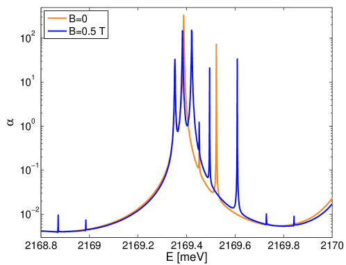
Figure 1: Changes in absorption spectrum due to the applied magnetic field for n=4 exciton.

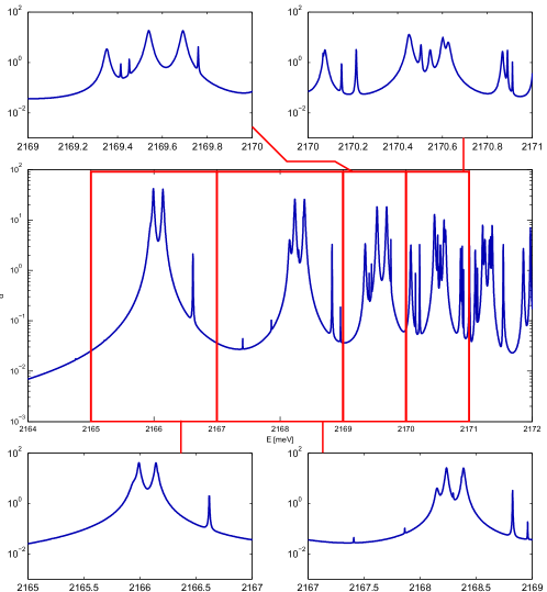
Figure 2: The bulk magnetoabsorption of Cu₂O crystal calculated from the imaginary part of the bulk susceptibility (37) for $B$=2T. Insets show the detailed spectra around the excitonic lines corresponding to n=4, 5, 6, 7.

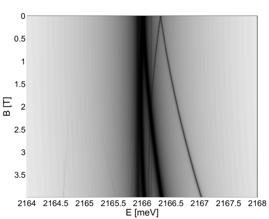
Figure 3: Absorption spectrum in the energetic region of $n=4$ excitonic state as a function of the applied magnetic field strength.

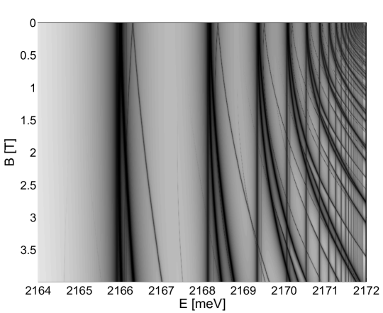
Figure 4: Te same as in Fig 3, in the energetic region of $n=4-25$ excitonic states.

IV Second iteration step - magneto-optic functions

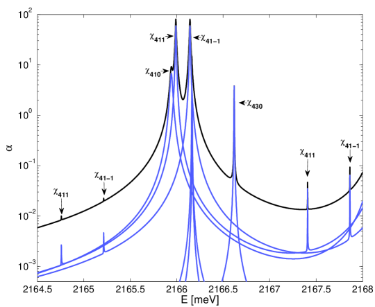
Figure 5: The bulk magnetoabsorption of Cu₂O crystal, individual excitonic resonances are identified.

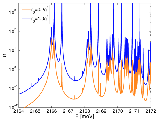
Figure 6: The influence of the choice of the coherence radius $r_{0}$ on the magnetoabsorption spectra of Cu₂O crystal.

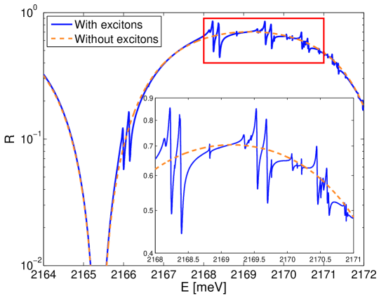
Figure 7: The magneto-reflection coefficient of Cu₂O crystal of thickness 30 $\mu\hbox{m}$, when the magnetic field 2T is applied. The dashed curve (labelled without excitons) corresponds to Fabry-Perot reflection. Inset - reflection spectrum for n=5, 6, 7 exciton.

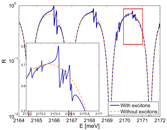
Figure 8: The same as in Fig. 7, for crystal thickness 100 $\mu\hbox{m}$. Inset - reflection spectrum for n=7 exciton.

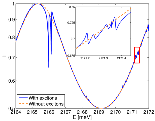
Figure 9: The transmissivity coefficient of Cu₂O crystal of thickness 30 $\mu\hbox{m}$, when the magnetic field 2T is applied. The dashed curve (labelled without excitons) corresponds to Fabry-Perot transmissivity. Inset - transmission spectrum for n=7 exciton.

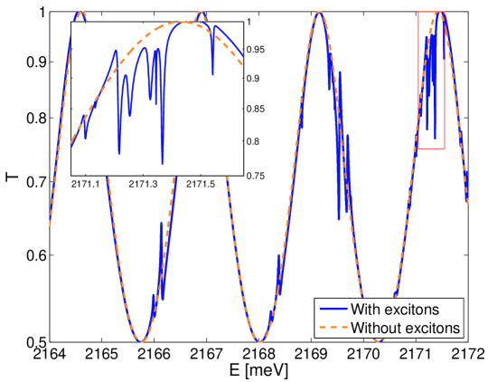
Figure 10: The same as in Fig. 9, for crystal thickness 100 $\mu\hbox{m}$. Inset - transmission spectrum for n=7 exciton.

In the first iteration step we have computed the coefficients $c_{Nn\ell m}$. Having them, we determine the amplitude $Y(Z,\textbf{r})$ from Eq. (9) and the excitonic polarization from the Eq. (13), obtaining

$$P_{\rm exc}(Z) = 2\int M^{*}(\textbf{r})Y(Z,\textbf{r}){\rm d}^{3}r=2\int M^{*}(\textbf{r})\sum\limits_{Nn\ell m}c_{Nn\ell m}R_{n\ell m}Y_{\ell m}w_{N}(Z){\rm d}^{3}r=\sum\limits_{N}P_{N}w_{N}(Z),$$

$$P_{N} = 2\sum\limits_{n\ell m}c_{Nn\ell m}\langle M^{*}|R_{n\ell m}Y_{\ell m}\rangle=\epsilon_{0}\epsilon_{b}\Delta_{LT}^{(P)}\langle w_{N}|E_{\rm hom}(Z)\rangle\sum_{n\ell m}\chi_{Nn\ell m}$$

$$=\epsilon_{0}\epsilon_{b}\Delta_{LT}^{(P)}I_{N}E_{\rm hom}(0)\sum_{n\ell m}\chi_{Nn\ell m},$$

where $I_{N}$ are defined in Eq. (72), and $\chi_{Nn\ell m}$ in Eqn. (F, F). The so obtained polarization will be used as a source in the Maxwell equation (12). As is known, the solution of a nonhomogeneous differential equation is composed of two parts, which are the solution of a homogeneous equation and of the nonhomogeneous one:

$$E(Z)=E_{\rm hom}(Z)+E_{\rm nhom}(Z),$$ (29)

where the homogeneous part satisfies the equation (16). The nonhomogeneous part will be obtained by means of the appropriate Green function, satisfying the equation

$$\frac{{\rm d}^{2}}{{\rm d}Z^{2}}G^{E}(Z,Z^{\prime})+k_{b}^{2}G^{E}(Z,Z^{\prime})=-\delta(Z-Z^{\prime}),$$ (30)

and having the form (for example, RivistaGC )

$$G^{E}(Z,Z^{\prime}) = \frac{\rm i}{2k_{b}W}\left(e^{-{\rm i}k_{b}Z^{<}}+\frac{k_{b}-k_{0}}{k_{b}+k_{0}}e^{{\rm i}k_{b}Z^{<}}\right)$$ (31)

$$\times \left(\frac{k_{b}-k_{0}}{k_{b}+k_{0}}e^{{\rm i}k_{b}L-{\rm i}k_{b}Z^{>}}+e^{-{\rm i}k_{b}L+{\rm i}k_{b}Z^{>}}\right),$$

where $Z^{<}=\hbox{min}(Z,Z^{\prime}),Z^{>}=\hbox{max}(Z,Z^{\prime})$. Using the above Green’s function we obtain the nonhomogeneous part in the form

$$E_{\rm nhom}(Z)=\frac{k_{0}^{2}}{\epsilon_{0}}\int\limits_{0}^{L}G^{E}(Z,Z^{\prime})P_{\rm exc}(Z^{\prime}){\rm d}Z^{\prime}.$$ (32)

The equations (29), (31), and (32) give the total electric field of the wave propagating in the crystal, from which the reflectivity $R$ and transmissivity $T$ are obtained. They have the form

$$R = \left|\frac{E(0)}{E_{\rm in}}-1\right|^{2}$$

$$=R_{\rm FP}\Biggl{|}1+{\rm i}\left(\frac{k_{b}L}{2}\right)\frac{(1-r_{\infty}^{2})(1-r_{\infty}e^{{\rm i}\Theta})^{2}(1-r_{\infty}^{2}e^{{\rm i}\Theta})}{r_{\infty}(1-e^{{\rm i}\Theta})}\sum\limits_{N}\left(\frac{I_{N}^{2}}{L}\right)\sum\limits_{n\ell m}\Delta_{LT}^{(P)}\chi_{Nn\ell m}\Biggr{|}^{2},$$

$$T = \left|\frac{E(L)}{E_{\rm in}}\right|^{2}=T_{\rm FP}\left|1+{\rm i}\left(\frac{E}{2E_{L}}\right)\frac{(1-r_{\infty}e^{{\rm i}\Theta})}{(1-r_{\infty}^{2}e^{{\rm i}\Theta})}\sum\limits_{N}\left(\frac{I_{N}^{2}}{L}\right)\sum\limits_{n\ell m}\Delta_{LT}^{(P)}\chi_{Nn\ell m}\right|^{2},$$ (34)

where $\Theta=2k_{b}L$, $r_{\infty}$ is defined by

$$r_{\infty}=\frac{k_{0}-k_{b}}{k_{0}+k_{b}},$$ (35)

$I_{n}^{2}/L$ are given in Eq. (73), and $R_{\rm FP},T_{\rm FP}$ are the well-known formulas for the Fabry-Perot normal incidence reflectivity and transmissivity of a lossless dielectric slab of thickness $L$ (see, e.g., Klingshirn ),

$$R_{\rm FP} = \frac{F\sin^{2}(\Theta/2)}{1+F\sin^{2}(\Theta/2)},\quad T_{\rm FP}=\frac{1}{1+F\sin^{2}(\Theta/2)},$$

$$F = \frac{4r_{\infty}^{2}}{(1-r_{\infty}^{2})^{2}}.$$ (36)

The derivation of the formulas (IV) and (34) is given in Appendix E.

V Results

We have performed numerical calculations of magneto-optical functions (absorption, reflectivity, and transmissivity) for the Cu₂O crystal having in mind the experiments by Aßmann et al assmann . Considering the specific properties of Cu₂O and the crystal dimension large compared to the exciton Bohr radius, we observe that the COM quantized energies $W_{N}$ (II) are small compared to the remaining components of the excitonic energies $W_{Nn\ell m}$ (III). Therefore, in the first approximation, we can neglect them in the formulas defining the coefficients $c_{Nn\ell m}$ (Appendix A) and in expressions $\chi_{Nn\ell m}$ (F,F), and calculate the bulk magneto-susceptibility

$$\chi(\omega) = \epsilon_{b}\Delta_{LT}^{(P)}\left[\chi_{N211}+\chi_{N21-1}+\chi_{N311}+\chi_{N31-1}+\chi_{Nn3\pm 3}+\tilde{\chi}_{Nn1\pm 1}+\tilde{\chi}_{Nn3\pm 1}\ldots\right],$$ (37)

Using the formula $\alpha=(\omega/c)\hbox{Im}\,\sqrt{\epsilon_{b}+\chi}$ we have calculated the magneto-absorption, taking into account the lowest $n=2-10$ excitonic states. The parameters we used are the energies $E_{n\ell m}$, the gap energy $E_{g}$, the L-T energy $\Delta_{LT}^{(P)}$, and the dissipation parameter $\mit\Gamma$. We have used the electron and hole effective masses: $m_{e}=1.01,m_{h\parallel}=0.5587,\mu_{\parallel}=0.3597,\mu_{z}=0.672\;\hbox{(the masses in free electron mass)}\;m_{0}$, from them calculated the reduced mass $\mu_{\parallel}^{\prime}=-1.25$, which gives ${\mu_{\parallel}}/{\mu_{\parallel}^{\prime}}\approx-0.2876.$ Since the LT splitting for P excitons is not known, we have established a relation between the known $\Delta_{LT}$ for S excitons and the quantity $\Delta_{LT}^{(P)}$ for P excitons. First, using the bulk dispersion

$$\frac{c^{2}k^{2}}{\omega^{2}}=\epsilon_{b}+\frac{2}{\epsilon_{0}}\int{\rm d}^{3}rM^{*}Y,$$ (38)

for $k=0,n=2$, we establish the relation between the splitting and the dipole matrix element

$$\epsilon_{b}\Delta_{LT}^{(P)} = \left.\frac{2}{\epsilon_{0}}\left|I_{1}+I_{2}\right|^{2}\left[\frac{1}{W_{111}}+\frac{1}{W_{11-1}}\right]\right|_{B=0},$$

$$\left|M_{10}\right|^{2} = \frac{4\epsilon_{0}\epsilon_{b}a^{*3}\Delta_{LT}^{(P)}}{\pi(r_{0}/a^{*})^{2}\eta_{11}^{5}},$$ (39)

where $I_{1},I_{2}$ are defined in Eq.(B,53). Using an analogous expression for for S excitons (Zeitschrift )

$$\left|M_{10}\right|^{2}=\frac{\pi\epsilon_{0}\epsilon_{b}a^{*3}\Delta_{LT}^{(S)}}{\eta_{00}^{3}}$$

one can determine $\Delta_{LT}^{(P)}$ as function of $\Delta_{LT}^{(S)}$

$$\Delta_{LT}^{(P)} = \frac{\pi^{2}}{4}\left(\frac{r_{0}}{a^{*}}\right)^{2}\frac{\eta_{11}^{5}}{\eta_{00}^{3}}\Delta_{LT}^{(S)}.$$ (40)

The energies $W_{Nn\ell m}$ were obtained from the relations (11), and (III) (without $W_{N}$) with the effective Rydberg energy $R^{*}$. We have used the values $E_{g}=2172\leavevmode\nobreak\ \hbox{meV},R^{*}=86.981\leavevmode\nobreak\ \hbox{meV}$, $\Delta^{(S)}_{LT}=10\leavevmode\nobreak\ \mu\hbox{eV}$ which is common value in available literature, $\mu_{\parallel}/\mu_{z}=0.5351$, and phenomenological value of damping ${\mit\Gamma}=0.1\leavevmode\nobreak\ \hbox{meV}$. We have restricted the upper limit of energy for our numerical illustrations to $2172\leavevmode\nobreak\ \hbox{meV}$, which determines the band gap; above this energy one could take into account effects which follow from interaction with the continuous spectrum. The results for the absorption, which seem the most important, are reported in Figs. 1-6. In Fig. 1 we observe how the applied magnetic field changes the spectra. The positions of absorption maxima are changed due to the diamagnetic shift, and the Zeeman splitting occurs. The same effects, for a larger number of excitonic states and stronger field, are displayed in Fig. 2. For the principal quantum number $n\geq 4$ the effects due to both P and F excitons, for example, the overlapping of states, are observed. This is shown in Fig. 3 for the $n=4$ exciton state, where the dependence of the absorption on the applied field strength is shown. The Zeeman splitting is clearly visible and the lines are shifted towards higher energy with increasing field strength. Moreover, some absorption lines become visible only for sufficiently strong magnetic field. Our calculation scheme can be extended to higher principal quantum number; the absorption spectrum for n=4-25 excitonic states is shown on the Fig. 4. In Fig. 5 we show that our method allows to identify the excitonic states. In the RDMA approach we consider the role of the coherence of the radiation field with excitons, which enters via the smeared dipole density M(r) and its parameters $\textbf{M}_{0},r_{0}$. The influence of the coherence radius $r_{0}$ is illustrated in Fig. 6. One can observe that an increase of $r_{0}$ causes an increase of absorption, which is due to the related increase of the L-T splitting and oscillator strength, see Eq. (40). The COM quantization approximation, used in our calculations, allowed to calculate the reflection and transmission spectra, taking into account both the microscopic electronic excitations (excitons) and their interaction with the radiation field, resulting in creation of polariton modes. We have obtained analytical expressions for the reflection coefficient $R$ and the transmissivity $T$, and their shapes are shown in Figs. 7-10. The calculation has been performed up to N=350 and for excitonic states with principal number n=4-7. One can observe the overlapping of the Fabry-Perot modes, typical for a dielectric slab, with excitonic resonances. Notably, the Fabry-Perot interference has the dominating effect, strongly affecting the reflection and transmission coefficient over the whole energy range. Conversely, the variation of reflection coefficient due to the excitonic resonances has a comparably small amplitude, but is quickly varying with energy. In the Fig. 7 inset, one can see that these two effects are readily separable.

VI Conclusions

The main results of our paper can be summarized as follows. We have proposed a procedure based on the RDMA approach that allows to obtain analytical expressions for the magneto-optical functions of semiconductor crystals including high number Rydberg excitons. Our results have general character because arbitrary exciton angular momentum number and arbitrary applied field strength are included. We have chosen the example of cuprous oxide, inspired by the recent experiment by Aßmann et al assmann . We have calculated the magneto-optical functions (susceptibility, absorption, reflection, and transmission), obtaining a fairly good agreement between the calculated and the experimentally observed spectra.

As each method using iterative procedure presented approach is a kind of approximation. Although we have solved the problem of excitons in semiconductor when an external magnetic field is applied, but we do not include the interaction between states with different n into the Hamiltonian we have used. It should emphasized that presented approach is analytical until the last step in which the numerical code is used. The choice of dipole density model and therefore the oscillator strengths, which is intricate function of free parameters has an impact on accuracy of our calculations and might be the source of discrepancy between the experimental results. Our results confirm the fundamental peculiarity of magneto-optical effects: shifting, splitting and, as a result for higher excitonic states, mixing of spectral lines. In particular, we obtained the splitting of P and F excitons, with increasing number of peaks corresponding to the increasing state number. All these interesting features of excitons with high $n$ number which are examined and discussed on the basis on our theory might possibly provide deep insight into the nature of Rydberg excitons in solids and provoke their application to design all-optical flexible switchers and future implementation in quantum information processing.

Appendix A Expansion coefficients $c_{Nn\ell m}$

Using the eigenfunctions (II) and transition dipole densities (21), (22) we calculate the expansion coefficients $c_{Nn\ell m}$. For $n=2,3$ we only hace the coefficients related to the $P$ excitons:

$$W_{N_{1}n1\pm 1}c_{N_{1}n1\pm 1}+V^{(n)}_{11\pm 1}c_{N_{1}n1\pm 1} = \langle w_{N_{1}}|E_{x}\rangle\langle R_{211}Y_{1\pm 1}|M_{x}^{(1)}\rangle,$$

$$c_{N_{1}n1\pm 1} = \frac{\langle w_{N_{1}}|E_{x}\rangle\langle R_{n11}Y_{1\pm 1}|M_{x}^{(1)}\rangle}{W_{N_{1}n1\pm 1}+V^{(n)}_{11\pm 1}}.$$ (41)

For $n\geq 4$ we must consider contributions of both excitons $P$ and $F$. For $n=4$ we have three equations

$$W_{N_{1}41\pm 1}c_{N_{1}41\pm 1}+V^{(4)}_{11\pm 1}c_{N_{1}41\pm 1}+V^{(4)}_{13\pm 1}c_{N_{1}43\pm 1}=\langle w_{N_{1}}|E_{x}\rangle\langle R_{411}Y_{1\pm 1}|M^{(1)}_{x}\rangle,$$

$$W_{N_{1}43\pm 1}c_{N_{1}43\pm 1}+V^{(4)}_{33\pm 1}c_{N_{1}43\pm 1}+V^{(4)}_{31\pm 1}c_{N_{1}41\pm 1}=\langle w_{N_{1}}|E_{x}\rangle\langle R_{431}Y_{3\pm 1}|M^{(3)}_{x}\rangle,$$ (42)

$$W_{N_{1}43\pm 3}c_{N_{1}43\pm 3}+V^{(4)}_{33\pm 3}c_{N_{1}43\pm 3}=\langle w_{N_{1}}|E_{x}\rangle\langle R_{433}Y_{3\pm 3}|M^{(3)}_{x}\rangle.$$

The first two equations can be put into the form

$$a_{11}c_{N_{1}41\pm 1}+a_{12}c_{N_{1}43\pm 1}=b_{1},$$

$$a_{21}c_{N_{1}41\pm 1}+a_{22}c_{N_{1}43\pm 1}=b_{2},$$

$$a_{11}=W_{N_{1}41\pm 1}+V^{(4)}_{11\pm 1},$$ (43)

$$a_{12}=V^{(4)}_{13\pm 1}=a_{21},$$

$$a_{22}=W_{N_{1}43\pm 1}+V^{(4)}_{33\pm 1},$$

$$b_{1}=\langle w_{N_{1}}|E_{x}\rangle\langle R_{411}Y_{1\pm 1}|M^{(1)}_{x}\rangle,$$

$$b_{2}=\langle w_{N_{1}}|E_{x}\rangle\langle R_{431}Y_{3\pm 1}|M^{(3)}_{x}\rangle,$$

with solutions

$$c_{N_{1}41\pm 1} = \langle w_{N_{1}}|E_{x}\rangle\frac{a_{22}\langle R_{411}Y_{1\pm 1}|M^{(1)}_{x}\rangle-a_{12}\langle R_{431}Y_{3\pm 1}|M^{(3)}_{x}\rangle}{\Delta},$$

$$c_{N_{1}43\pm 1} = \langle w_{N_{1}}|E_{x}\rangle\frac{a_{11}\langle R_{431}Y_{3\pm 1}|M^{(3)}_{x}\rangle-a_{12}\langle R_{411}Y_{1\pm 1}|M^{(1)}_{x}\rangle}{\Delta},$$ (44)

$$\Delta = a_{11}a_{22}-a_{12}^{2}.$$

The third of equations (A) has the solution in the form

$$c_{N_{1}43\pm 3}=\frac{\langle w_{N_{1}}|E_{x}\rangle\langle R_{433}Y_{3\pm 3}|M^{(3)}_{x}\rangle}{W_{N_{1}43\pm 3}+V^{(4)}_{33\pm 3}}.$$ (45)

For $n=5$ we obtain quite analogous equations

$$W_{N_{1}51\pm 1}c_{N_{1}51\pm 1}+V^{(5)}_{11\pm 1}c_{N_{1}51\pm 1}+V^{(5)}_{13\pm 1}c_{N_{1}53\pm 1}=\langle w_{N_{1}}|E_{x}\rangle\langle R_{511}Y_{1\pm 1}|M^{(1)}_{x}\rangle,$$

$$W_{N_{1}53\pm 1}c_{N_{1}53\pm 1}+V^{(5)}_{33\pm 1}c_{N_{1}53\pm 1}+V^{(5)}_{31\pm 1}c_{N_{1}51\pm 1}=\langle w_{N_{1}}|E_{x}\rangle\langle R_{531}Y_{3\pm 1}|M^{(3)}_{x}\rangle,$$ (46)

$$W_{N_{1}53\pm 3}c_{N_{1}53\pm 3}+V^{(5)}_{33\pm 3}c_{N_{1}53\pm 3}=\langle w_{N_{1}}|E_{x}\rangle\langle R_{533}Y_{3\pm 3}|M^{(3)}_{x}\rangle.$$

The third of the above equations yields

$$c_{N_{1}53\pm 3}=\frac{\langle w_{N_{1}}|E_{x}\rangle\langle R_{533}Y_{3\pm 3}|M^{(3)}_{x}\rangle}{W_{N_{1}53\pm 3}+V^{(5)}_{33\pm 3}},$$ (47)

whereas the first two give the coefficients $c_{N_{1}51\pm 1},c_{N_{1}53\pm 1}$

$$c_{N_{1}5\pm 1} = \langle w_{N_{1}}|E_{x}\rangle\frac{a_{22}\langle R_{511}Y_{1\pm 1}|M^{(1)}_{x}\rangle-a_{12}\langle R_{531}Y_{3\pm 1}|M^{(3)}_{x}\rangle}{a_{11}a_{22}-a_{12}^{2}},$$

$$c_{N_{1}53\pm 1} = \langle w_{N_{1}}|E_{x}\rangle\frac{a_{11}\langle R_{531}Y_{3\pm 1}|M^{(3)}_{x}\rangle-a_{12}\langle R_{511}Y_{1\pm 1}|M^{(1)}_{x}\rangle}{a_{11}a_{22}-a_{12}^{2}},$$ (48)

where

$$a_{11}=W_{N_{1}51\pm 1}+V^{(5)}_{11\pm 1},$$

$$a_{12}=V^{(5)}_{13\pm 1}=a_{21},$$

$$a_{22}=W_{N_{1}53\pm 1}+V^{(5)}_{33\pm 1}.$$

In a similar way the higher order coefficients can be determined:

$$c_{N_{1}n3\pm 3} = \frac{\langle w_{N_{1}}|E_{x}\rangle\langle R_{n33}Y_{3\pm 3}|M^{(3)}_{x}\rangle}{W_{N_{1}n3\pm 3}+V^{(n)}_{33\pm 3}},$$

$$c_{N_{1}n1\pm 1} = \langle w_{N_{1}}|E_{x}\rangle\frac{a_{22}\langle R_{n11}Y_{1\pm 1}|M^{(1)}_{x}\rangle-a_{12}\langle R_{n31}Y_{3\pm 1}|M^{(3)}_{x}\rangle}{a_{11}a_{22}-a_{12}^{2}},$$ (49)

$$c_{N_{1}n3\pm 1} = \langle w_{N_{1}}|E_{x}\rangle\frac{a_{11}\langle R_{n31}Y_{3\pm 1}|M^{(3)}_{x}\rangle-a_{12}\langle R_{n11}Y_{1\pm 1}|M^{(1)}_{x}\rangle}{a_{11}a_{22}-a_{12}^{2}},$$

$$a_{11} = W_{N_{1}n1\pm 1}+V^{(n)}_{11\pm 1},$$

$$a_{12} = V^{(n)}_{13\pm 1}=a_{21},$$

$$a_{22} = W_{N_{1}n3\pm 1}+V^{(n)}_{33\pm 1},$$

$$\Delta = a_{11}a_{22}-a_{12}^{2}$$

$$c_{N_{1}n1\pm 1}=\frac{\langle w_{N_{1}}|E_{x}\rangle}{\Delta}\left\{a_{22}\left[\mp\sqrt{\frac{8\pi}{3}}\frac{M_{10}}{2{\rm i}}\left(\frac{r_{0}}{a^{*}}\right)\frac{\eta_{11}^{5/2}}{a^{*3/2}}\sqrt{\frac{n^{2}-1}{n^{5}}}\right]\right.$$

$$\left.-a_{12}\left[\mp 0.015272\cdot\sqrt{\frac{2}{3}\pi}M_{10}\left(\frac{r_{0}}{a^{*}}\right)^{3}\frac{\eta_{31}^{9/2}}{a^{*3/2}}\sqrt{\frac{(n^{2}-9)(n^{2}-4)(n^{2}-1)}{n^{9}}}\right]\right\}$$

$$=\frac{\langle w_{N_{1}}|E_{x}\rangle}{\Delta}\left(\frac{r_{0}}{a^{*}}\right)\sqrt{\frac{2}{3}\pi}M_{10}\frac{1}{a^{*3/2}}\sqrt{\frac{n^{2}-1}{n^{5}}}\left\{\pm a_{22}{\rm i}\eta_{11}^{5/2}\pm a_{12}\cdot 0.015272\cdot\left(\frac{r_{0}}{a^{*}}\right)^{2}\eta_{31}^{9/2}\sqrt{\frac{(n^{2}-9)(n^{2}-4)}{n^{4}}}\right\}$$

$$=\pm\frac{\langle w_{N_{1}}|E_{x}\rangle}{\left(W_{N_{1}n1\pm 1}+V^{(n)}_{111}\right)\left(W_{N_{1}n3\pm 1}+V^{(n)}_{331}\right)-\left(V^{(n)}_{131}\right)^{2}}\left(\frac{r_{0}}{a^{*}}\right)\sqrt{\frac{2}{3}\pi}M_{10}\frac{1}{a^{*3/2}}\sqrt{\frac{n^{2}-1}{n^{5}}}$$

$$\times\left\{{\rm i}\eta_{11}^{5/2}\left(W_{N_{1}n3\pm 1}+V^{(n)}_{331}\right)+0.015272\cdot V^{(n)}_{131}\left(\frac{r_{0}}{a^{*}}\right)^{2}\eta_{31}^{9/2}\sqrt{\frac{(n^{2}-9)(n^{2}-4)}{n^{4}}}\right\}$$

$$c_{N_{1}n3\pm 1}=\langle w_{N_{1}}|E_{x}\rangle\frac{a_{11}\langle R_{n31}Y_{3\pm 1}|M^{(3)}_{x}\rangle-a_{12}\langle R_{n11}Y_{1\pm 1}|M^{(1)}_{x}\rangle}{a_{11}a_{22}-a_{12}^{2}}$$

$$=\frac{\langle w_{N_{1}}|E_{x}\rangle}{\Delta}\left\{a_{11}\left[\mp 0.015272\cdot\sqrt{\frac{2}{3}\pi}M_{10}\left(\frac{r_{0}}{a^{*}}\right)^{3}\frac{\eta_{31}^{9/2}}{a^{*3/2}}\sqrt{\frac{(n^{2}-9)(n^{2}-4)(n^{2}-1)}{n^{9}}}\right]\right.$$

$$\left.-a_{12}\left[\mp\sqrt{\frac{8\pi}{3}}\frac{M_{10}}{2{\rm i}}\left(\frac{r_{0}}{a^{*}}\right)\frac{\eta_{11}^{5/2}}{a^{*3/2}}\sqrt{\frac{n^{2}-1}{n^{5}}}\right]\right\}$$

$$=\mp\frac{\langle w_{N_{1}}|E_{x}\rangle}{\Delta}\left(\frac{r_{0}}{a^{*}}\right)\sqrt{\frac{2}{3}\pi}M_{10}\frac{1}{a^{*3/2}}\sqrt{\frac{n^{2}-1}{n^{5}}}$$

$$\left\{a_{11}\cdot 0.015272\cdot\left(\frac{r_{0}}{a^{*}}\right)^{2}\eta_{31}^{9/2}\sqrt{\frac{(n^{2}-9)(n^{2}-4)}{n^{4}}}+a_{12}{\rm i}\eta_{11}^{5/2}\right\}$$

$$=\mp\frac{\langle w_{N_{1}}|E_{x}\rangle}{\left(W_{N_{1}n1\pm 1}+V^{(n)}_{111}\right)\left(W_{N_{1}n3\pm 1}+V^{(n)}_{331}\right)-\left(V^{(n)}_{131}\right)^{2}}\left(\frac{r_{0}}{a^{*}}\right)\sqrt{\frac{2}{3}\pi}M_{10}\frac{1}{a^{*3/2}}\sqrt{\frac{n^{2}-1}{n^{5}}}$$

$$\times\left\{\left[W_{N_{1}n1\pm 1}+V^{(n)}_{111}\right]\cdot 0.015272\cdot\left(\frac{r_{0}}{a^{*}}\right)^{2}\eta_{31}^{9/2}\sqrt{\frac{(n^{2}-9)(n^{2}-4)}{n^{4}}}\right.$$

$$\left.+V^{(n)}_{131}\cdot{\rm i}\eta_{11}^{5/2}\right\}$$

Appendix B Determination of the quantities $\langle R_{n11}Y_{1\pm 1}|M^{(1)}_{x}\rangle,\langle R_{n31}Y_{3\pm 1}|M^{(3)}_{x}\rangle,\langle R_{n33}Y_{3\pm 3}|M^{(3)}_{x}\rangle$

Below we calculate the quantities $\langle R_{n11}Y_{1\pm 1}|M^{(1)}_{x}\rangle,\langle R_{n31}Y_{3\pm 1}|M^{(3)}_{x}\rangle,\langle R_{n33}Y_{3\pm 3}|M^{(3)}_{x}\rangle$, which enter in the above derived formulas for the coefficients $c_{Nn\ell m}$. Using the definition (21, 22) one obtains

$$\langle R_{n11}Y_{1\pm 1}|M_{x}^{(1)}x\rangle = \mp\sqrt{\frac{8\pi}{3}}\frac{M_{10}}{4{\rm i}r_{0}^{2}}\int\limits_{0}^{\infty}r^{2}{\rm d}r\;\frac{r+r_{0}}{r^{2}}e^{-r/r_{0}}R_{n11}(r).$$ (50)

Inserting on the r.h.s. the expression for the radial function $R_{n11}$ (see Eq. (II)) we get

$$\langle R_{n11}Y_{1\pm 1}|M_{x}^{(1)}x\rangle = \mp\sqrt{\frac{8\pi}{3}}\frac{M_{10}}{4{\rm i}r_{0}^{2}}\int\limits_{0}^{\infty}{\rm d}r\;(r+r_{0})e^{-\lambda r}\left(\frac{2\eta_{11}}{na^{*}}\right)^{3/2}\frac{1}{3!}\sqrt{\frac{(n+1)!}{2n(n-2)!}}$$ (51)

$$\times\left(\frac{2\eta_{11}r}{na^{*}}\right)M\left(-n+2,4,\frac{2\eta_{11}r}{na^{*}}\right),$$

where

$$\lambda = \frac{1}{r_{0}}+\frac{\eta_{11}}{na^{*}}=\frac{na^{*}+\eta_{11}r_{0}}{na^{*}r_{0}}.$$

The r.h.s. of Eq. (51) consists of two parts:

$$I_{1}=\sqrt{\frac{8\pi}{3}}\frac{M_{10}}{4{\rm i}r_{0}^{2}}\left(\frac{2\eta_{11}}{na^{*}}\right)^{3/2}\left(\frac{2\eta_{11}}{na^{*}}\right)\frac{1}{3!}\sqrt{\frac{(n+1)!}{2n(n-2)!}}\int\limits_{0}^{\infty}{\rm d}r\;r^{2}\,e^{-\lambda r}$$

$$\times M\left(-n+2,4,\frac{2\eta_{11}r}{na^{*}}\right)$$ (52)

$$=\sqrt{\frac{8\pi}{3}}\frac{M_{10}}{4{\rm i}r_{0}^{2}}\left(\frac{2\eta_{11}}{na^{*}}\right)^{5/2}\frac{1}{3!}\sqrt{\frac{(n+1)!}{2n(n-2)!}}\Gamma(3)\lambda^{-3}F\left(-n+2,3,4,\frac{2\eta_{11}r_{0}}{na^{*}+\eta_{11}r_{0}}\right),$$

$$I_{2}=\sqrt{\frac{8\pi}{3}}\frac{M_{10}}{4{\rm i}r_{0}^{2}}r_{0}\left(\frac{2\eta_{11}}{na^{*}}\right)^{5/2}\frac{1}{3!}\sqrt{\frac{(n+1)!}{2n(n-2)!}}$$ (53)

$$\times\int\limits_{0}^{\infty}r{\rm d}r\;e^{-\lambda r}M\left(-n+2,4,\frac{2\eta_{11}}{na^{*}}\cdot r\right)$$

$$=\sqrt{\frac{8\pi}{3}}\frac{M_{10}}{4{\rm i}r_{0}^{2}}r_{0}\lambda^{-2}\left(\frac{2\eta_{11}}{na^{*}}\right)^{5/2}\frac{1}{3!}\sqrt{\frac{(n+1)!}{2n(n-2)!}}F\left(-n+2,2,4,\frac{2\eta_{11}r_{0}}{na^{*}+\eta_{11}r_{0}}\right),$$

$F(\alpha,\beta,\gamma,z)$ being the hypergeometric series (for example, Grad )

$$F=1+\frac{\alpha\beta}{\gamma}\,\frac{z}{1!}+\frac{\alpha(\alpha+1)\beta(\beta+1)}{\gamma(\gamma+1)}\,\frac{z^{2}}{2!}+\ldots.$$ (54)

Performing the summation we obtain

$$I_{1}+I_{2}=\sqrt{\frac{8\pi}{3}}\frac{M_{10}}{4{\rm i}r_{0}^{2}}\left(\frac{2\eta_{11}}{na^{*}}\right)^{5/2}\frac{1}{3!}\sqrt{\frac{(n+1)!}{2n(n-2)!}}2\lambda^{-3}F\left(-n+2,3,4,\frac{2\eta_{11}r_{0}}{na^{*}+\eta_{11}r_{0}}\right)$$

$$+\sqrt{\frac{8\pi}{3}}\frac{M_{10}}{4{\rm i}r_{0}^{2}}r_{0}\lambda^{-2}\left(\frac{2\eta_{11}}{na^{*}}\right)^{5/2}\frac{1}{3!}\sqrt{\frac{(n+1)!}{2n(n-2)!}}F\left(-n+2,2,4,\frac{2\eta_{11}r_{0}}{na^{*}+\eta_{11}r_{0}}\right)$$

$$\approx\sqrt{\frac{8\pi}{3}}\frac{M_{10}}{4{\rm i}r_{0}^{2}}\left(\frac{2\eta_{11}}{na^{*}}\right)^{5/2}\frac{1}{3!}\sqrt{\frac{(n+1)!}{2n(n-2)!}}\frac{n^{2}a^{*2}r_{0}^{3}(3na^{*}+\eta_{11}r_{0})}{(na^{*}+\eta_{11}r_{0})^{3}}$$

$$=\sqrt{\frac{8\pi}{3}}\frac{M_{10}r_{0}}{8{\rm i}}\left(\frac{2\eta_{11}}{na^{*}}\right)^{5/2}\sqrt{\frac{(n+1)!}{2n(n-2)!}},$$

where the assumption $r_{0}<a^{*}$ has been used. Finally

$$\langle R_{n11}Y_{1\pm 1}|M_{x}^{(1)}\rangle=\mp\sqrt{\frac{2\pi}{3}}\frac{M_{10}}{{\rm i}}\left(\frac{r_{0}}{a^{*}}\right)\frac{\eta_{11}^{5/2}}{a^{*3/2}}\sqrt{\frac{n^{2}-1}{n^{5}}}.$$ (55)

The following expression will be useful in calculation of oscillator strengths

$$\left|I_{1}+I_{2}\right|^{2}=\frac{2}{3}\pi\left|M_{10}\right|^{2}\left(\frac{r_{0}}{a^{*}}\right)^{2}\frac{\eta_{11}^{5}}{a^{*3}}\frac{n^{2}-1}{n^{5}}.$$ (56)

In the next step we calculate the quantity $\langle R_{n31}Y_{3\pm 1}|M_{x}^{(3)}x\rangle$. Using the definitions (III) and (II) one obtains

$$\langle R_{n31}Y_{3\pm 1}|M_{x}^{(3)}x\rangle=\mp\sqrt{\frac{3\pi}{7}}\frac{M_{10}}{r_{0}}\int\limits_{0}^{\infty}{\rm d}r\;e^{-r/r_{0}}R_{n31}(r)$$

$$=\mp\sqrt{\frac{3\pi}{7}}\frac{M_{10}}{r_{0}}\left(\frac{2\eta_{31}}{na^{*}}\right)^{9/2}\int\limits_{0}^{\infty}{\rm d}r\;r^{3}\,e^{-\lambda r}\frac{1}{7!}\sqrt{\frac{(n+3)!}{2n(n-4)!}}$$

$$\times M\left(-n+4,8,\frac{2\eta_{31}}{na^{*}}\cdot r\right)$$

with

$$\lambda=\frac{1}{r_{0}}+\frac{\eta_{31}}{na^{*}}=\frac{na^{*}+\eta_{31}r_{0}}{na^{*}r_{0}}.$$

Performing the integration we arrive at the formulas

$$\langle R_{n31}Y_{3\pm 1}|M_{x}^{(3)}\rangle=\mp\sqrt{\frac{3\pi}{7}}\frac{M_{10}}{r_{0}}\left(\frac{2\eta_{31}}{na^{*}}\right)^{9/2}\sqrt{\frac{(n+3)!}{2n(n-4)!}}\,\frac{3!}{7!}\lambda^{-4}\,F\left(-n+4,4,8,\frac{2\eta_{31}}{na^{*}\lambda}\right)$$

$$=\mp\sqrt{\frac{3\pi}{7}}\frac{M_{10}}{r_{0}}\left(\frac{2\eta_{31}}{na^{*}}\right)^{9/2}\sqrt{\frac{(n+3)!}{2n(n-4)!}}\,\frac{3!}{7!}\frac{n^{4}a^{*4}r_{0}^{4}}{(na^{*}+\eta_{31}r_{0})^{4}}\,F\left(-n+4,4,8,\frac{2\eta_{31}}{na^{*}\lambda}\right)$$

$$\approx\mp\;0.015272\cdot\sqrt{\frac{2}{3}\pi}M_{10}\left(\frac{r_{0}}{a^{*}}\right)^{3}\frac{\eta_{31}^{9/2}}{a^{*3/2}}\sqrt{\frac{(n^{2}-9)(n^{2}-4)(n^{2}-1)}{n^{9}}},$$

where again the assumption $r_{0}<a^{*}$ has been used. The formula

$$\left|\langle R_{n31}Y_{3\pm 1}|M_{x}^{(3)}\rangle\right|^{2}\approx\frac{3\pi}{2\cdot 7}\frac{|M_{10}|^{2}}{a^{*3}}\left(\frac{3!}{7!}\right)^{2}\left(2\eta_{31}\right)^{9}\left(\frac{r_{0}}{a^{*}}\right)^{6}\frac{(n^{2}-9)(n^{2}-4)(n^{2}-1)}{n^{9}}$$

$$=2.332\cdot 10^{-4}\frac{2}{3}\pi\frac{|M_{10}|^{2}}{a^{*3}}\left(\eta_{31}\right)^{9}\left(\frac{r_{0}}{a^{*}}\right)^{6}\frac{(n^{2}-9)(n^{2}-4)(n^{2}-1)}{n^{9}}$$

will be used in calculations of the oscillator strengths related to the F exciton. The remaining formulas, connected to the $Y_{3,\pm 3}$ harmonics, have the form

$$\langle R_{n33}Y_{3\pm 3}|M_{x}^{(3)}\rangle=\mp\sqrt{\frac{5\pi}{7}}\frac{M_{10}}{r_{0}}\left(\frac{2\eta_{33}}{na^{*}}\right)^{9/2}\sqrt{\frac{(n+3)!}{2n(n-4)!}}\,\frac{3!}{7!}\lambda^{-4}\,F\left(-n+4,4,8,\frac{2\eta_{33}}{na^{*}\lambda}\right)$$

$$\left|\langle R_{n33}Y_{3\pm 3}|M_{x}^{(3)}\rangle\right|^{2}\approx\frac{5\pi}{2\cdot 7}\frac{|M_{10}|^{2}}{a^{*3}}\left(\frac{3!}{7!}\right)^{2}\left(2\eta_{33}\right)^{9}\left(\frac{r_{0}}{a^{*}}\right)^{6}\frac{(n^{2}-9)(n^{2}-4)(n^{2}-1)}{n^{9}}$$ (57)

$$=3.887\cdot 10^{-4}\frac{2}{3}\pi\frac{|M_{10}|^{2}}{a^{*3}}\left(\eta_{33}\right)^{9}\left(\frac{r_{0}}{a^{*}}\right)^{6}\frac{(n^{2}-9)(n^{2}-4)(n^{2}-1)}{n^{9}}.$$

Appendix C Derivation of the matrix elements $V^{(nn_{1})}_{\ell\ell_{1}mm_{1}}$

In order to calculate the matrix elements $V^{(nn_{1})}_{\ell\ell_{1}mm_{1}}$, as defined in Eq. (25), we start with the integral containing the angular dependence

$$I_{\ell\ell_{1}mm_{1}} = \langle Y_{\ell_{1}m_{1}}|\sin^{2}\theta|Y_{\ell m}\rangle=\int{\rm d}\Omega\;Y^{*}_{\ell_{1}m_{1}}(1-\cos^{2}\theta)Y_{\ell m}$$ (58)

$$= \delta_{\ell\ell_{1}}\delta_{mm_{1}}-\int{\rm d}\Omega\;Y_{\ell_{1}m_{1}}\cos^{2}\theta\,Y_{\ell m}.$$

Making use of the definition of the spherical harmonic functions

$$Y_{\ell m}(\theta,\phi)=\sqrt{\frac{(2\ell+1)(\ell-m)!}{4\pi(\ell+m)!}}P^{m}_{\ell}(\cos\theta)e^{{\rm i}m\phi},$$ (59)

in terms of the associated Legendre polynomials $P^{m}_{\ell}$, the second of the integrals on the r.h.s. of Eq. (58) can be put into the form

$$I = \int{\rm d}\Omega\;Y_{\ell_{1}m_{1}}^{*}\cos^{2}\theta\,Y_{\ell m}$$

$$=\delta_{mm_{1}}2\pi\sqrt{\frac{(2\ell+1)(\ell-m)!}{4\pi(\ell+m)!}\frac{(2\ell_{1}+1)(\ell_{1}-m_{1})!}{4\pi(\ell_{1}+m_{1})!}}\int\limits_{-1}^{+1}{\rm d}x\,P^{m}_{\ell}(x)x^{2}P^{m_{1}}_{\ell_{1}}(x).$$

Making use of the recurrence relation (Grad )

$$xP^{m}_{\ell}(x)=\frac{1}{2\ell+1}\left[(\ell-m+1)P^{m}_{\ell+1}(x)+(\ell+m)P^{m}_{\ell-1}(x)\right],$$ (61)

we arrive at the integral

$$\int\limits_{-1}^{+1}{\rm d}x\,P^{m}_{\ell}(x)x^{2}P^{m_{1}}_{\ell_{1}}(x)=\int\limits_{-1}^{+1}{\rm d}x\biggl{\{}\frac{1}{2\ell+1}\left[(\ell-m+1)P^{m}_{\ell+1}(x)+(\ell+m)P^{m}_{\ell-1}(x)\right]$$

$$\times\;\frac{1}{2\ell_{1}+1}\left[(\ell_{1}-m+1)P^{m}_{\ell_{1}+1}(x)+(\ell_{1}+m)P^{m}_{\ell_{1}-1}(x)\right]\biggr{\}}.$$ (62)

Performing the multiplication and integration, using the orthogonality relation

$$\int\limits_{-1}^{+1}P^{m}_{\ell}(x)P^{m}_{\ell_{1}}(x){\rm d}x=\frac{2}{2\ell+1}\frac{(\ell+m)!}{(\ell-m)!}\delta_{\ell\ell_{1}},$$

one obtains

$$\int\limits_{-1}^{+1}{\rm d}x\,P^{m}_{\ell}(x)x^{2}P^{m_{1}}_{\ell_{1}}(x)=\frac{2(2\ell^{2}+2\ell-1-2m^{2})(\ell+m)!}{(2\ell-1)(2\ell+1)(2\ell+3)(\ell-m)!}\delta_{\ell\ell_{1}}$$

$$+\frac{2(\ell-m+1)(\ell+m+2)(\ell+m+1)!}{(2\ell+1)(2\ell+3)(2\ell+5)(\ell+1-m)!}\delta_{\ell+1,\ell_{1}-1}$$ (63)

$$+\frac{2(\ell-m-1)(\ell+m)(\ell+m-1)!}{(2\ell-3)(2\ell-1)(2\ell+1)(\ell-1-m)!}\delta_{\ell_{1}+1,\ell-1}.$$

The above result inserting into the Eq. (C) gives for the angular integration

$$I = \delta_{mm_{1}}2\pi\sqrt{\frac{(2\ell+1)(\ell-m)!}{4\pi(\ell+m)!}\frac{(2\ell_{1}+1)(\ell_{1}-m_{1})!}{4\pi(\ell_{1}+m_{1})!}}$$

$$\times\;\biggl{[}\frac{2(2\ell^{2}+2\ell-1-2m^{2})(\ell+m)!}{(2\ell-1)(2\ell+1)(2\ell+3)(\ell-m)!}\delta_{\ell\ell_{1}}$$

$$+\frac{2(\ell-m+1)(\ell+m+2)(\ell+m+1)!}{(2\ell+1)(2\ell+3)(2\ell+5)(\ell+1-m)!}\delta_{\ell+1,\ell_{1}-1}$$

$$+\frac{2(\ell-m-1)(\ell+m)(\ell+m-1)!}{(2\ell-3)(2\ell-1)(2\ell+1)(\ell-1-m)!}\delta_{\ell_{1}+1,\ell-1}\biggr{]}.$$

Using the above results we obtain the diagonal matrix element $V^{nn_{1}}_{\ell\ell_{1}mm_{1}}$ when $n=n_{1}$

$$V^{n}_{\ell_{1}\ell_{1}m_{1}m_{1}} = \frac{R^{*}}{4}\gamma^{2}\delta_{\ell\ell_{1}mm_{1}}\left(1-\frac{2\ell_{1}^{2}+2\ell_{1}-1-2m_{1}^{2}}{(2\ell_{1}-1)(2\ell_{1}+3)}\right)\int\limits_{0}^{\infty}{\rm d}\rho\rho^{4}\,R_{n\ell}R_{n_{1}\ell_{1}}$$

$$= \delta_{\ell\ell_{1}mm_{1}}\frac{R^{*}}{4}\gamma^{2}\frac{2(\ell^{2}+\ell+m^{2}-1)}{(2\ell-1)(2\ell+3)}\int\limits_{0}^{\infty}{\rm d}\rho\,\rho^{4}\,\left[R_{n\ell}(\rho)\right]^{2}$$

$$= \delta_{\ell\ell_{1}mm_{1}}\frac{R^{*}}{4}\gamma^{2}\frac{(\ell^{2}+\ell+m^{2}-1)}{(2\ell-1)(2\ell+3)}\left(\frac{n}{\eta_{\ell m}}\right)^{2}[5n^{2}+1-3\ell(\ell+1)]$$

where we used the formula (for example Messiah where $\eta_{\ell m}=1$)

$$\langle\rho^{2}\rangle=\frac{1}{2}[5n^{2}+1-3\ell(\ell+1)].$$ (66)

In a similar way the the off-diagonal elements can be computed with the results displayed in Eq. (III). The integrals containing the radial eigenfunctions $R_{n\ell m}$ can be expressed by the integrals over Laguerre polynomials

$$I_{n\ell sm}=\int\limits_{0}^{\infty}{\rm d}\rho\rho^{4}\,R_{n\ell m}R_{nsm}=\int\limits_{0}^{\infty}{\rm d}\rho\rho^{4}\left(\frac{2\eta_{\ell m}}{n}\right)^{3/2}\sqrt{\frac{(n-\ell-1)!}{2n(n+\ell)!}}\left(\frac{2\eta_{\ell m}\rho}{n}\right)^{\ell}$$

$$\times L_{n-\ell-1}^{2\ell+1}\left(\frac{2\eta_{\ell m}\rho}{n}\right)e^{-\eta_{\ell m}\rho/n}$$

$$\times\left(\frac{2\eta_{\ell m}}{n}\right)^{3/2}\sqrt{\frac{(n-s-1)!}{2n(n+s)!}}\left(\frac{2\eta_{\ell m}\rho}{n}\right)^{s}\,L_{n-s-1}^{2s+1}\left(\frac{2\eta_{\ell m}\rho}{n}\right)e^{-\eta_{\ell m}\rho/n}$$

$$=\left(\frac{n}{2\eta_{\ell m}}\right)^{2}\sqrt{\frac{(n-\ell-1)!}{2n(n+\ell)!}}\sqrt{\frac{(n-s-1)!}{2n(n+s)!}}\int\limits_{0}^{\infty}x^{\ell+s+4}L_{n-\ell-1}^{2\ell+1}(x)L_{n-s-1}^{2s+1}(x)e^{-x}{\rm d}x$$

For example, taking $n=4,\ell=1,s=3,m=1$, one has

$$I_{4131} = \int\limits_{0}^{\infty}{\rm d}\rho\rho^{4}\,R_{411}R_{431}=\left(\frac{4}{2\eta_{10}}\right)^{2}\sqrt{\frac{2!}{2\cdot 4\cdot 5!}}\sqrt{\frac{0!}{2\cdot 4\cdot 7!}}\int\limits_{0}^{\infty}x^{8}L_{2}^{3}(x)L_{0}^{7}(x)e^{-x}{\rm d}x$$

$$=\left(\frac{2}{\eta_{10}}\right)^{2}\sqrt{\frac{1}{4\cdot 5!}}\sqrt{\frac{1}{8!}}\int\limits_{0}^{\infty}x^{8}\frac{1}{2}\left[x^{2}-10x+20\right]e^{-x}{\rm d}x$$

$$=\left(\frac{1}{\eta_{10}}\right)^{2}\,8!\sqrt{\frac{1}{5!8!}}\left(90-90+20\right)=20\left(\frac{1}{\eta_{10}}\right)^{2}\sqrt{\frac{8!}{5!}}\approx 367\left(\frac{1}{\eta_{10}}\right)^{2}.$$

Appendix D Calculation of the coefficients $\langle w_{N}|E\rangle$

The homogeneous solution of the field equation (III) can be put into the form

$$E_{\rm hom}(Z)=Ae^{{\rm i}k_{b}Z}+Be^{-{\rm i}k_{b}Z},$$ (67)

where

$$A = \frac{2k_{0}}{(k_{0}+k_{b})W}e^{-{\rm i}k_{b}L}E_{\rm in},$$

$$B = \frac{2k_{0}(k_{b}-k_{0})}{(k_{0}+k_{b})^{2}W}e^{{\rm i}k_{b}L}E_{\rm in}.$$ (68)

With these expressions one obtains for $\langle w_{N}|E\rangle$

$$\langle w_{N}|E\rangle=AI+BI^{*},$$ (69)

with the notation

$$I=\langle w_{N}|\,e^{{\rm i}k_{b}Z}\rangle=\sqrt{\frac{2}{L}}\int\limits_{0}^{L}\sin\frac{N\pi}{L}Z\,e^{{\rm i}k_{b}Z}\,{\rm d}Z.$$ (70)

With the use of the relations

$$\sin x=\frac{e^{{\rm i}x}-e^{-{\rm i}x}}{2{\rm i}},\quad e^{\pm{\rm i}N\pi}=\cos N\pi,$$ (71)

the integral $I$ becomes

$$I=I_{N}=\sqrt{2L}\left(1-\cos\,N\pi\exp\left[{\rm i}k_{b}{L}\right]\right)\frac{N\pi}{(N\pi)^{2}-(k_{b}L)^{2}}.$$ (72)

The quantity $I_{N}^{2}/L$ which appears in the expressions for the optical functions, has the form

$$\frac{I_{N}^{2}}{L}=\frac{2N^{2}\pi^{2}}{\left[\left(k_{b}L\right)^{2}-N^{2}\pi^{2}\right]^{2}}\left(1-\cos\,N\pi\exp\left[{\rm i}k_{b}{L}\right]\right)^{2}.$$ (73)

The expression $k_{b}L$ can be transformed in the following way:

$$k_{b}L = \frac{\hbar\omega}{\hbar c}\sqrt{\epsilon_{b}}L=\frac{E}{E_{L}},$$

$$E_{L} = \frac{\hbar c}{\sqrt{\epsilon_{b}}L}=\frac{0.66\cdot 10^{-15}\hbox{eV s}\cdot 3\cdot 10^{8}\hbox{m/s}}{\sqrt{\epsilon_{b}}L}$$ (74)

$$= \frac{1.98\cdot 10^{2}\hbox{meV}\cdot\mu\hbox{m}}{\sqrt{\epsilon_{b}}L(\mu\hbox{m})}.$$

For the Cu₂O data $\epsilon_{b}=7.5$ and

$$E_{L}=\frac{72.3}{L}\,\hbox{meV},$$ (75)

where $L$ is expressed in $\mu\hbox{m}$. For $L=30\,\mu\hbox{m}$ we have $E_{L}=2.41\,\hbox{meV}$. Since $I_{N}=I_{N}^{*}$, it follows from (69)

$$\langle w_{N}|E_{\rm hom}(Z)\rangle=I_{N}(A+B)=I_{N}E_{\rm hom}(0),$$ (76)

where

$$E_{\rm hom}(0) = \frac{2k_{0}}{(k_{0}+k_{b})W}E_{\rm in}\left(e^{-{\rm i}k_{b}L}+\frac{k_{b}-k_{0}}{k_{b}+k_{0}}e^{{\rm i}k_{b}L}\right)$$

$$= E_{\rm in}\frac{1+r_{\infty}}{1-r_{\infty}^{2}\exp({\rm i}\Theta)}\left(1-r_{\infty}e^{{\rm i}\Theta}\right).$$

Appendix E Optical functions

Below we derive the formulas (IV) and (34). They will be obtained from Eq. (III) by using the total electric field $E(Z)=E_{\rm hom}(Z)+E_{\rm nhom}(Z)$. In particular, for the reflection coefficient one obtains

$$R=|r|^{2},$$ (78)

with

$$r = r_{0}+r_{\rm exc},$$

$$r_{0} = \frac{r_{\infty}\left(1-e^{{\rm i}\Theta}\right)}{1-r_{\infty}^{2}e^{{\rm i}\Theta}},$$ (79)

$$r_{\rm exc} = \frac{k_{0}^{2}}{\epsilon_{0}E_{\rm in}}\int\limits_{0}^{L}\,G^{E}(0,Z)P_{\rm exc}(Z){\rm d}Z.$$

Since

$$G^{E}(0,Z)=\frac{{\rm i}(1-r_{\infty})}{2k_{b}\left(1-r_{\infty}^{2}\,e^{{\rm i}\Theta}\right)}\left(e^{{\rm i}k_{b}Z}-r_{\infty}\,e^{{\rm i}\Theta-{\rm i}k_{b}Z}\right),$$ (80)

we obtain

$$r_{\rm exc}=\frac{k_{0}^{2}}{\epsilon_{0}E_{\rm in}}\int\limits_{0}^{L}\,G^{E}(0,Z)P_{\rm eks}(Z){\rm d}Z$$

$$=\frac{k_{0}^{2}}{\epsilon_{0}E_{\rm in}}\frac{{\rm i}(1-r_{\infty})}{2k_{b}\left(1-r_{\infty}^{2}\,e^{{\rm i}\Theta}\right)}\sum\limits_{N}\int\limits_{0}^{L}\,\left(e^{{\rm i}k_{b}Z}-r_{\infty}\,e^{{\rm i}\Theta-{\rm i}k_{b}Z}\right)P_{N}w_{N}(Z){\rm d}Z$$ (81)

$$=\frac{k_{0}^{2}}{2\epsilon_{0}E_{\rm in}}\frac{{\rm i}(1-r_{\infty})}{k_{b}\left(1-r_{\infty}^{2}\,e^{{\rm i}\Theta}\right)}\sum\limits_{N}\left[\langle w_{N}|e^{{\rm i}k_{b}Z}\rangle-r_{\infty}\,e^{{\rm i}\Theta}\langle w_{N}|e^{-{\rm i}k_{b}Z}\rangle\right]P_{N}$$

$$=\frac{k_{0}^{2}}{2\epsilon_{0}E_{\rm in}}\frac{{\rm i}(1-r_{\infty})}{k_{b}\left(1-r_{\infty}^{2}\,e^{{\rm i}\Theta}\right)}\left(1-r_{\infty}\,e^{{\rm i}\Theta}\right)\sum\limits_{N}I_{N}P_{N},$$

from which, with respect to Eqn. (IV), we get

$$r_{\rm exc} = \frac{k_{0}^{2}E_{\rm hom}(0)}{2E_{\rm in}}\frac{{\rm i}(1-r_{\infty})}{k_{b}\left(1-r_{\infty}^{2}\,e^{{\rm i}\Theta}\right)}\left(1-r_{\infty}\,e^{{\rm i}\Theta}\right)\epsilon_{b}\sum\limits_{N}I_{N}^{2}\sum\limits_{n\ell m}\Delta_{LT}^{(P)}\chi_{Nn\ell m}.$$ (82)

Inserting in the above equation the expression (D), we obtain

$$r_{{\rm exc}} = \frac{\epsilon_{b}k_{0}^{2}}{2k_{b}}\frac{{\rm i}(1-r^{2}_{\infty})}{\left(1-r_{\infty}^{2}\,e^{{\rm i}\Theta}\right)^{2}}\left(1-r_{\infty}\,e^{{\rm i}\Theta}\right)^{2}\sum\limits_{N}{I_{N}^{2}}\sum\limits_{n\ell m}\Delta_{LT}^{(P)}\chi_{Nn\ell m}$$ (83)

$$=\frac{\rm i}{2}\,\frac{(k_{b}L)(1-r^{2}_{\infty})}{\left(1-r_{\infty}^{2}\,e^{{\rm i}\Theta}\right)^{2}}\left(1-r_{\infty}\,e^{{\rm i}\Theta}\right)^{2}\sum\limits_{N}\left(\frac{I_{N}^{2}}{L}\right)\sum\limits_{n\ell m}\Delta_{LT}^{(P)}\chi_{Nn\ell m}.$$

Now the total complex reflection coefficient $r$ obtains the form

$$r = r_{0}+r_{\rm exc}=r_{0}\Biggl{[}1+{\rm i}\left(\frac{E}{2E_{L}}\right)\frac{(1-r_{\infty}^{2})(1-r_{\infty}e^{{\rm i}\Theta})^{2}(1-r_{\infty}^{2}e^{{\rm i}\Theta})}{r_{\infty}(1-e^{{\rm i}\Theta})}$$ (84)

$$\times\sum\limits_{N}\left(\frac{I_{N}^{2}}{L}\right)\sum\limits_{n\ell m}\Delta_{LT}^{(P)}\chi_{Nn\ell m}\Biggr{]},$$

which, using the Eq. (78) immediately gives the result (IV).

Analogically, we determine the transmissivity

$$T=\left|\frac{E(L)}{E_{\rm in}}\right|^{2},$$ (85)

resulting from the equation

$$T=|t|^{2},$$ (86)

where

$$t = t_{0}+t_{\rm exc},$$

$$t_{0} = \frac{1-r_{\infty}^{2}}{1-r_{\infty}^{2}e^{{\rm i}\Theta}}e^{{\rm i}\Theta/2},$$ (87)

$$t_{\rm exc} = \frac{k_{0}^{2}}{\epsilon_{0}E_{\rm in}}\int\limits_{0}^{L}\,G^{E}(L,Z)P_{\rm exc}(Z){\rm d}Z.$$

Since

$$G^{E}(L,Z)=\frac{\rm i}{2k_{b}W}\left(e^{-{\rm i}k_{b}Z}+\frac{k_{b}-k_{0}}{k_{b}+k_{0}}e^{{\rm i}k_{b}Z}\right)$$

$$\times\>\left(\frac{k_{b}-k_{0}}{k_{b}+k_{0}}e^{{\rm i}k_{b}L-{\rm i}k_{b}L}+e^{-{\rm i}k_{b}L+{\rm i}k_{b}L}\right)$$ (88)

$$=\frac{{\rm i}e^{{\rm i}\Theta/2}\left(1-r_{\infty}\right)}{2k_{b}\left(1-r_{\infty}^{2}e^{{\rm i}\Theta}\right)}\left(e^{-{\rm i}k_{b}Z}-r_{\infty}e^{{\rm i}k_{b}Z}\right),$$

we have

$$t_{{\rm exc}}=\frac{k_{0}^{2}}{E_{\rm in}}\int\limits_{0}^{L}\,G^{E}(L,Z)P_{\rm exc}(Z){\rm d}Z$$

$$=\frac{(k_{b}L)}{2}\frac{{\rm i}e^{{\rm i}\Theta/2}\left(1-r_{\infty}\right)}{\left(1-r_{\infty}^{2}e^{{\rm i}\Theta}\right)^{2}}\left(1+r_{\infty}\right)\left(1-r_{\infty}\,e^{{\rm i}\Theta}\right)\sum\limits_{N}\left(\frac{I_{N}^{2}}{L}\right)\sum\limits_{n\ell m}\Delta_{LT}^{(P)}\chi_{Nn\ell m},$$

and

$$t=t_{0}+t_{\rm exc}=t_{0}\left[1+\frac{1}{t_{0}}\frac{(k_{b}L)}{2}\frac{{\rm i}e^{{\rm i}\Theta/2}\left(1-r_{\infty}\right)}{\left(1-r_{\infty}^{2}e^{{\rm i}\Theta}\right)^{2}}\left(1+r_{\infty}\right)\left(1-r_{\infty}\,e^{{\rm i}\Theta}\right)\sum\limits_{N}\left(\frac{I_{N}^{2}}{L}\right)\sum\limits_{n\ell m}\Delta_{LT}^{(P)}\chi_{Nn\ell m}\right]$$

$$=t_{0}\left[1+{\rm i}\left(\frac{E}{2E_{L}}\right)\frac{(1-r_{\infty}e^{{\rm i}\Theta})}{(1-r_{\infty}^{2}e^{{\rm i}\Theta})}\sum\limits_{N}\left(\frac{I_{N}^{2}}{L}\right)\sum\limits_{n\ell m}\Delta_{LT}^{(P)}\chi_{Nn\ell m}\right].$$ (89)

Inserting the above result into Eq. (86), we obtain the transmissivity (34).

Appendix F Derivation of the quantities $\chi_{Nn\ell m}$

Using the dispersion relation

$$\frac{c^{2}k^{2}}{\omega^{2}}=\epsilon_{b}+\frac{2}{\epsilon_{0}}\int{\rm d}^{3}rM^{*}Y,$$

$$\frac{2}{\epsilon_{0}}\int{\rm d}^{3}rM^{*}Y=\frac{2}{\epsilon_{0}}\int{\rm d}^{3}rM_{x}^{(1)*}\sum_{n\ell m}c_{Nn\ell m}R_{n\ell m}Y_{\ell m}$$ (90)

$$+\frac{2}{\epsilon_{0}}\int{\rm d}^{3}rM_{x}^{(3)*}\sum_{n\ell m}c_{Nn\ell m}R_{n\ell m}Y_{\ell m}$$

we define the quantities $\chi_{Nn\ell m}$ and $\tilde{\chi}_{Nn\ell m}$ :

$$\frac{2}{\epsilon_{0}}\int{\rm d}^{3}rM^{(1)*}_{x}c_{N_{1}n1\pm 1}R_{n11}Y_{1\pm 1} = \epsilon_{b}\Delta_{LT}^{(P)}\tilde{\chi}_{N_{1}n1\pm 1}\langle E_{x}|w_{N_{1}}\rangle$$

$$\frac{2}{\epsilon_{0}}\int{\rm d}^{3}rM^{(3)*}_{x}c_{N_{1}n3\pm 1}R_{n31}Y_{3\pm 1} = \epsilon_{b}\Delta_{LT}^{(P)}\tilde{\chi}_{N_{1}n3\pm 1}\langle E_{x}|w_{N_{1}}\rangle$$ (91)

$$\frac{2}{\epsilon_{0}}\int{\rm d}^{3}rM^{(3)*}_{x}c_{N_{1}n3\pm 3}R_{n33}Y_{3\pm 3} = \epsilon_{b}\Delta_{LT}^{(P)}\tilde{\chi}_{N_{1}n3\pm 3}\langle E_{x}|w_{N_{1}}\rangle.$$

The notation $\tilde{\chi}$ denotes that the formula contains contributions from both excitons P and F. Using the formulas (21,22), and the expressions $\langle R_{n11}Y_{1\pm 1}|M^{(1)}_{x}\rangle,\langle R_{n31}Y_{3\pm 1}|M^{(3)}_{x}\rangle,\langle R_{n33}Y_{3\pm 3}|M^{(3)}_{x}\rangle$ derived in Appendix B, we obtain obtaining the following formulas: for n=2,3

$$\chi_{Nn1\pm 1} = \frac{f_{n11}}{W_{n1\pm 1}+V^{(n)}_{11\pm 1}}$$

$$f_{n11} = \frac{16}{3}\frac{n^{2}-1}{n^{5}}.$$ (92)

For $n\geq 4$ we observe the overlapping of the P and F excitons, which is reflected in the formulas

$$\chi_{Nn3\pm 3} = \frac{f_{n33}}{W_{Nn3\pm 3}+V^{(n)}_{33\pm 3}},$$

$$f_{n33} = 2.073\cdot 10^{-3}\;\frac{\eta_{33}^{9}}{\eta_{11}^{5}}\left(\frac{r_{0}}{a^{*}}\right)^{4}\frac{(n^{2}-9)(n^{2}-4)(n^{2}-1)}{n^{9}},$$

$$\tilde{\chi}_{Nn1\pm 1} = \frac{16}{3}\frac{n^{2}-1}{n^{5}}\frac{1}{\left(W_{Nn1\pm 1}+V^{(n)}_{111}\right)\left(W_{Nn3\pm 1}+V^{(n)}_{331}\right)-\left(V^{(n)}_{131}\right)^{2}}$$

$$\times\,\left\{\left(W_{Nn3\pm 1}+V^{(n)}_{331}\right)-{\rm i}\cdot\,0.015272\cdot V^{(n)}_{131}\left(\frac{r_{0}}{a^{*}}\right)^{2}\frac{\eta_{31}^{9/2}}{\eta_{11}^{5/2}}\sqrt{\frac{(n^{2}-9)(n^{2}-4)}{n^{4}}}\right\},$$

$$\tilde{\chi}_{Nn3\pm 1} = 0.015272\frac{16}{3}\left(\frac{r_{0}}{a^{*}}\right)^{2}\frac{\eta_{31}^{9/2}}{\eta_{11}^{5}}\frac{n^{2}-1}{n^{5}}\sqrt{\frac{(n^{2}-9)(n^{2}-4)}{n^{4}}}$$

$$\times\frac{1}{\left(W_{Nn1\pm 1}+V^{(n)}_{111}\right)\left(W_{Nn3\pm 1}+V^{(n)}_{331}\right)-\left(V^{(n)}_{131}\right)^{2}}$$

$$\times\Biggl{\{}\left[W_{Nn1\pm 1}+V^{(n)}_{111}\right]\cdot 0.015272\cdot\left(\frac{r_{0}}{a^{*}}\right)^{2}\eta_{31}^{9/2}\sqrt{\frac{(n^{2}-9)(n^{2}-4)}{n^{4}}}+{\rm i}\cdot\,V^{(n)}_{131}\cdot\eta_{11}^{5/2}\Biggr{\}}.$$

References

- (1) Ya. J. Frenkel, Phys. Rev. 37, 17 ; 37, 1276 (1931).
- (2) G. H. Wannier, Phys. Rev. 52, 191 (1937).
- (3) N. F. Mott, Trans. Faraday Soc. 34, 500 (1938).
- (4) E. F. Gross and N. A. Karriiev, Dokl. Akad. Nauk SSSR 84, 471 (1952).
- (5) R. S. Knox, Theory of Excitons (Academic Press, New York, 1963).
- (6) V. M. Agranovich and V. L. Ginzburg, Crystal Optics with spatial Dispersion and Excitons (Springer Verlag, Berlin, 1984).
- (7) A. Stahl and I. Balslev, Electrodynamics of the Semiconductor Band Edge (Springer-Verlag, Berlin-Heidelberg-New York, 1987).
- (8) G. La Rocca, Wannier-Mott Excitons in Semiconductors. In: Electronic Excitations in Organic Based Nanostructures, ed. by V. M. Agranovich and G. F. Bassani, Thin Films and Nanostructures, vol. 31, Elsevier, Amsterdam, 2003, pp. 97-128.
- (9) G. Czajkowski, F. Bassani, and L. Silvestri, Rivista del Nuovo Cimento 26, 1-150 (2003).
- (10) V. M. Agranovich, Excitations in Organic Solids (Oxford University Press, Oxford, 2009).
- (11) C. Weisbuch and B. Vinter, Quantum Semiconductor Structures: Fundamentals and Applications (Academic Press, New York 1991).
- (12) L. Banyai and S. W. Koch, Semiconductor Quantum Dots (World Scientific, Singapure 1993).
- (13) E. L. Ivchenko and G. E. Pikus, Superlattices and Other Heterostructures. Symmetry and Optical Phenomena (Springer Verlag, Berlin 1995).
- (14) L. Woggon, Optical Properties of Semiconductor Quantum Dots (Springer Verlag, Berlin 1997).
- (15) L. Jacak, P. Hawrylak, and A. Wojs, Quantum Dots (Springer Verlag, Berlin 1998).
- (16) D. Bimberg, M. Grundmann and N. N. Ledentsov, Quantum Dot Heterostructures (Wiley, New York 1998).
- (17) T. Chakraborty, Quantum Dots (Elsevier, Amsterdam 1999).
- (18) V. M. Ustinov, A. E. Zhukov, A. Yu. Egorov, and N. A. Maleev: Quantum Dot Lasers (Oxford Science Publ., Oxford University Press, Oxford 2003).
- (19) E. L. Wolf, Nanophysics and Nanotechnology, An Introduction to Modern Concepts in Nanoscience (Wiley, Weinheim 2004).
- (20) O. Manasreh, Semiconductor Heterojunctions and Nanostructures (McGraw-Hill, New York 2005).
- (21) P. Harrison, Quantum Wells, Wires and Dots (Wiley, New York 2005).
- (22) T. Kazimierczuk, D. Fröhlich, S. Scheel, H. Stolz, and M. Bayer, Nature 514, 344 (2014).
- (23) S. Höfling and A. Kavokin, Nature 514, 313 (2014).
- (24) J. Thewes, J. Heckötter, T. Kazimierczuk, M. Aßmann, D. Fröhlich, M. Bayer, M. A. Semina, and M. M. Glazov, Phys. Rev. Lett. 115, 027402 (2015).
- (25) J. Heckötter, Stark-Effect Measurements on Rydberg Excitons in Cu2O. Thesis. Technical University Dortmund, 2015.
- (26) S. Zielińska-Raczyńska, G. Czajkowski, and D. Ziemkiewicz, Phys. Rev. B 93, 075206 (2016).
- (27) F. Schweiner, J. Main, and G. Wunner, Phys. Rev. B 93, 085203 (2016)
- (28) F. Schöne, S.-O. Krüger, P. Grünwald, H. Stolz, M. Aßmann, J. Heckötter, J. Thewes, D. Fröhlich, and M. Bayer, Phys. Rev. B 93, 075203 (2016).
- (29) M. Feldmaier, J. Main, F. Schweiner, H. Cartarius, and G. Wunner, J. Phys. B: At. Mol. Opt. Phys. 49, 144002 (2016).
- (30) F. Schweiner, J. Main, M. Feldmaier, G. Wunner, and Ch. Uihlein, Phys. Rev. B 94, 115201 (2016).
- (31) M. Aßmann, J. Thewes, D. Frölich, and M. Bayer, Nature Materials, 15, 741 (2016).
- (32) P. Grünwald, M. Aßmann, J. Heckötter, D. Fröhlich, M. Bayer, H. Stolz, and S. Scheel, arXiv:1609.04278v1 [cond-mat.mes-hall], 14 Sep 2016.
- (33) S. Zielińska-Raczyńska, D. Ziemkiewicz, and G. Czajkowski, Phys. Rev. B 94, 045205 (2016).
- (34) F. Schweiner, J. Main, G. Wunner, and arXiv: 1609.04275v1 [cond-mat.mtl - sci], 14 Sep 2016.
- (35) F. Schweiner, J. Main, G. Wunner, and arXiv: 1609.04278v1 [cond-mat.mtl - sci], 14 Sep 2016..
- (36) J. Ningyuan, A. Georgakoupoulos, A. Ryou, N. Schine, A. Sommer, and J. Simon, Phys. Rev. A, 93, 041802(R), 2016.
- (37) H. Tuffigo, R. T. Cox, N. Magnea, Y. Merle , and A. Million, Phys. Rev. B 37, 4310 (1988).
- (38) D, Andrea and R. Del Sole, Phys. Rev. B 41, 1413 (1990).
- (39) A. Tredicucci, Y. Chen, F. Bassani, J. Massies, C. Deparis, and G. Neu, Phys. Rev. B 47, 10348 (1993).
- (40) L. C. Andreani, Optical Transitions, Excitons and Polaritons in Bulk and Low-Dimensional Semiconductor Nanostructures. In: Confined Electrons and Photons, New Physics and Applications, ed. by E. Burstein and C. Weisbuch, pp. 57-112 (Plenum Press, New York, 1995 DOI 10.007/978-1-4615-1963-8, 1995).
- (41) N. Tomassini, A. D, Andrea, R. Del Sole, H. Tuffigo-Ulmer, and R. T. Cox, Phys. Rev. B 51, 5005 (1995).
- (42) P. Lefebvre, V. Calvo, N. Magnea, J. Allègre, T. Taliercio, and H. Mathieu, J. Cryst. Growth 184/185, 844 (1998).
- (43) D. Dragoman and M. Dragoman, Optical Characterization of Solids (Springer, Berlin-Heidelberg, ISBN 978-3-642-07521-6, 2002).
- (44) J. J. Davies, D. Wolverson, V. P. Kochereshko, A. V. Platonov, R. T. Cox, J. Cibert, H. Mariette, C. Bodin, C. Gourgon, I. V. Ignatiev, E. V. Ubylvovk, Y. P. Efimov, and S. A. Eliseev, Phys. Rev. Lett. 97, 187403 (2006).
- (45) L. C. Smith, J. J. Davies, D. Wolverson, S. Crampin, R. T. Cox, J. Cibert, H. Mariette, V. P. Kochereshko, M. Wiater, G. Karczewski, and T. Wojtowicz, Phys. Rev. B 78, 085204 (2008).
- (46) V. P. Kochereshko, L. C. Smith, J. J. Davies, R. T. Cox, A. Platonov, D. Wolverson, H. Boukari, H. Mariette, J. Cibert, M. Wiater, T. Wojtowicz, and G. Karczewski, Phys. Stat. Sol. B 245, 1059 (2008).
- (47) Strong Light-Matter Coupling. From Atoms to Solid-State Systems, edited by A. Auffèves, D. Gerace, M. Richard, S. Portolan, M. de Franca Santos, L. Ch. Kwek, and Ch. Miniatura (Word. Sc. Publish., Singapore, 2014).
- (48) M. Abramowitz and I. Stegun, Handbook of Mathematical Functions (Dover Publications, New York, 1965).
- (49) I. S. Gradshteyn and I. M. Ryzhik, Table of Integrals, Series, and Products. Ed. by A. Jeffrey, 5th edition. (Academic Press, San Diego, 1994).
- (50) G. Czajkowski, F. Bassani, and A. Tredicucci, Phys. Rev. B 54, 2035 (1996).
- (51) P. Schillak, Eur. Phys. J. B 84, 17 (2011).
- (52) P. Schillak and G. Czajkowski, Eur. Phys. J. B 88, 253 (2015).
- (53) C. F. Klingshirn, Semiconductor Optics, 4th Ed. (Springer, Heidelberg, 1995, DOI 10.007/978-3-642-28362-8).
- (54) F. Bassani, G. Czajkowski, and A. Tredicucci, Z. Phys. B 98, 39 (1995).
- (55) A. Messiah, Quantum Mechanics (North-Holland, Amsterdam, 1961).