Generalized Kapchinskij-Vladimirskij Distribution and Beam Matrix for Phase-Space Manipulations of High-Intensity Beams

Abstract

In an uncoupled linear lattice system, the Kapchinskij-Vladimirskij (KV) distribution, formulated on the basis of the single-particle Courant-Snyder (CS) invariants, has served as a fundamental theoretical basis for the analyses of the equilibrium, stability, and transport properties of high-intensity beams for the past several decades. Recent applications of high-intensity beams, however, require beam phase-space manipulations by intentionally introducing strong coupling. In this Letter, we report the full generalization of the KV model by including all of the linear (both external and space-charge) coupling forces, beam energy variations, and arbitrary emittance partition, which all form essential elements for phase-space manipulations. The new generalized KV model yields spatially uniform density profiles and corresponding linear self-field forces as desired. The corresponding matrix envelope equations and beam matrix for the generalized KV model provide important new theoretical tools for the detailed design and analysis of high-intensity beam manipulations, for which previous theoretical models are not easily applicable.

For the past several decades, the well-known Courant-Snyder (CS) theory Courant and Snyder (1958) has served as a fundamental theoretical tool in designing and analyzing an uncoupled linear lattice system. One of the recent areas of investigation by the beam physics community, however, is to manipulate the beam phase-space by intentionally introducing strong coupling. The round-to-flat beam transformation Kim (2003); Sun et al. (2004); Burov et al. (2002); Piot et al. (2006); Stratakis (2016) and the transverse-to-longitudinal emittance exchange Cornacchia and Emma (2002); Ruan et al. (2011); Emma et al. (2006); Kim (2007) have been investigated for electron injectors. The generation of flat hadron beams has recently drawn significant attention in the context of optimizing emittance budgets in heavy ion synchrotrons Xiao et al. (2013); Groening et al. (2014), and improving space-charge and beam-beam luminosity limitations in colliders Burov (2013). For muon ionization cooling, special arrangements of solenoidal mangets are employed to achieve six-dimensional emittance reduction Derbenev and Johnson (2005); Stratakis and Palmer (2015).

Various attempts have been made to extend the uncoupled CS theory to the case of general linear coupled systems Teng (1971); Ripken (1970); Lebedev and Bogacz (2010); Wolski (2014). However, due to the lack of a proper CS invariant for the coupled dynamics, previous analyses did not retain the elegant mathematical structure present in the original CS theory. Recently, Qin et al. Qin et al. (2013, 2014) have identified the generalized CS invariant for the linear coupled systems including both solenoidal and skew-quadrupole magnets, and variation of beam energy along the reference orbit. For phase-space manipulations, solenoidal and skew-quadrupole magnets are frequently used to provide strong coupling, as mentioned previously. Moreover, the relativistic mass increase may be important when there is a rapid acceleration of low-energy beams.

For some of the beam manipulations, space-charge effects are non-negligible as well; hence in those cases, we require a further generalization that incorporates space-charge effects into linear coupling lattices. In the original CS theory, space-charge effects were considered by means of the Kapchinskij-Vladimirskij (KV) distribution Kapchinskij and Vladimirskij (1959). For an intense beam propagating trough an alternating-gradient lattice, the KV distribution is the only known exact solution to the nonlinear Vlasov-Maxwell equations Davidson and Qin (2001); Lund (2015), and it generates linear space-charge forces consistent with the CS theory. Through the concept of rms-equivalent beams Sacherer (1971); Reiser (2008); Lund (2015), the KV beam model remains the most important basic design tool for high-intensity beam transport, even in the presence of nonlinear space-charge contributions. Several generalizations have been proposed for the KV model in order that it can be applied to coupled systems as well Sacherer (1968); Chernin (1988); Borchardt et al. (1988); Barnard (1995); Qin et al. (2009); Qin and Davidson (2013). However, none of them incorporates the solenoids and skew-quadrupoles simultaneously with a proper CS invariant.

In this Letter, we report the first complete generalization of the KV model for the general linear coupled system, so that the model describes all of the important processes for transverse phase-space manipulations of high-intensity beams. Due to the existence of the generalized CS invariant, the KV model developed here provides a self-consistent solution to the nonlinear Vlasov-Maxwell equations for high-intensity beams in coupled lattices, and leads to a matrix version of the envelope equation with an elegant Hamiltonian structure. We emphasize that space-charge effects during emittance manipulation, illustrated by a numerical example in this Letter, is one area that previous KV models could not address.

First, we consider a transverse Hamiltonian in general linear focusing lattice of the form

$$H_{\perp}=\frac{1}{2}{\bf z}^{T}A_{c}(s){\bf z},~{}~{}~{}A_{c}(s)=\left[\begin{array}[]{cc}\kappa&R\\ R^{T}&m^{-1}\\ \end{array}\right].$$ (1)

Here, ${\bf z}=(x,y,p_{x},p_{y})^{T}$ denotes the transverse canonical coordinates, $s$ is the path length that plays the role of a time-like variable, and $\kappa$ and $m^{-1}$ are $2\times 2$ symmetric matrices. The arbitrary $2\times 2$ matrix $R$ is not symmetric in general. The canonical momenta are normalized by a fixed reference momentum $p_{0}=\gamma_{0}m_{b}\beta_{0}c$. Based on the generalized CS theory developed in Refs. Qin et al. (2013, 2014), we obtain the solution for the coupled dynamics governed by the Hamiltonian (1) in the form of a linear map ${\bf z}(s)=M(s){\bf z}_{0}$, where ${\bf z}_{0}$ is the initial condition and $M$ is the transfer matrix defined by

$$M(s)=Q^{-1}P^{-1}P_{0}Q_{0}=\left[\begin{array}[]{cc}W&0\\ V&W^{-T}\\ \end{array}\right]P^{T}\left[\begin{array}[]{cc}W^{-1}&0\\ -V^{T}&W^{T}\\ \end{array}\right]_{0},$$ (2)

where subscript “0” denotes initial conditions at $s=0$, $P^{T}=P^{-1}$ and $P$ is a symplectic rotation, and $P_{0}$ is set equal to the unit matrix $I$ without loss of generality. Here, the $2\times 2$ matrices $W$ and $V$ are defined by $W=w^{T}$ and $V=m\left(\frac{dw^{T}}{ds}-R^{T}w^{T}\right)$. Furthermore, the $2\times 2$ envelope matrix $w$ is obtained by solving the matrix envelope equation given by Qin et al. (2013, 2014)

$$\frac{d}{ds}\left(\frac{dw}{ds}m-wRm\right)+\frac{dw}{ds}mR^{T}+w(\kappa-RmR^{T})-\left(w^{T}wmw^{T}\right)^{-1}=0.$$ (3)

We note that the second-order matrix differential equation (3) can be expressed in terms of two first-order equations, i.e.,

$$W^{\prime}=m^{-1}V+R^{T}W,~{}~{}~{}V^{\prime}=-\kappa W-RV+\left(W^{T}mWW^{T}\right)^{-1}.$$ (4)

The variable $V$ can be considered to be the matrix associated with the envelope momentum Lee (2004). We also note that Eq. (4) has similar Hamiltonian structure to the single particle equations of motion except for the term $\left(W^{T}mWW^{T}\right)^{-1}$ [see Eq. (12) for comparison and Ref. Chung et al. (2016) for a more detailed discussion].

The $4\times 4$ phase advance matrix $P$ has the following form Qin et al. (2013, 2014)

$$P=\left[\begin{array}[]{rr}C_{o}&-S_{i}\\ S_{i}&C_{o}\\ \end{array}\right].$$ (5)

Here, $C_{o}$ and $S_{i}$ are the $2\times 2$ matrices that satisfy $C_{o}^{\prime}=-S_{i}\left(W^{T}mW\right)^{-1}$ and $S_{i}^{\prime}=+C_{o}\left(W^{T}mW\right)^{-1}$, where the term $\left(W^{T}mW\right)^{-1}$ represents the phase advance rate. From the symplecticity of $P$, we note that $S_{i}C_{o}^{T}=C_{o}S_{i}^{T}$ and $S_{i}S_{i}^{T}+C_{o}C_{o}^{T}=I$. The generalized CS invariant of the Hamiltonian (1) is given by $I_{\xi}={\bf z}^{T}Q^{T}P^{T}\xi PQ{\bf z},$ where $\xi$ is a constant $4\times 4$ matrix, which is both symmetric and positive definite. The $\xi$ matrix acquires a meaning associated with emittance when the beam distribution is defined in terms of the CS invariant $I_{\xi}$ [see, for example, Eq. (13)]. The two symplectic eigenvalues of $\xi$ are directly connected to the eigen-emittances of the beam Chung et al. (2013).

By using $s$ as an independent coordinate, and treating $|p_{x}-q_{b}A_{x}/p_{0}|,|p_{y}-q_{b}A_{y}/p_{0}|\ll p_{0}$ and $|q_{b}\phi^{sc}|\ll\gamma_{b}m_{b}c^{2}$, we can express the transverse Hamiltonian (normalized by $p_{0}$) to second order in the transverse momenta as Davidson and Qin (2001); Wolski (2014)

$$H_{\perp}=\frac{1}{2p_{b}/p_{0}}\left[\left(p_{x}-\frac{q_{b}A_{x}}{p_{0}}\right)^{2}+\left(p_{y}-\frac{q_{b}A_{y}}{p_{0}}\right)^{2}\right]+\left(\frac{1}{\gamma_{b}^{2}}\right)\frac{q_{b}\phi^{sc}}{\beta_{b}cp_{0}}-\frac{q_{b}A_{s}^{ext}}{p_{0}},$$ (6)

where we have used the fact that the longitudinal vector potential is composed of both external ($A_{s}^{ext}$) and self-field ($A_{s}^{sc}$) contributions, and the self-field potentials $\phi^{sc}$ and $A_{s}^{sc}$ are related approximately by $A_{s}^{sc}=\beta_{b}\phi^{sc}/c$. Also, it is assumed that the reference trajectory is a straight line, that the longitudinal motion is independent of the transverse motion, and that there is no external electric focusing. Furthermore, $p_{b}(s)=\gamma_{b}m_{b}\beta_{b}c$, $\gamma_{b}(s)$, and $\beta_{b}(s)$ are regarded as prescribed functions of $s$ set by the acceleration schedule of the beamline Lund (2015). Hence, for a combination of the quadrupole, skew-quadrupole, and solenoidal fields, we obtain the following matrices for the Hamiltonian (1)

$$\kappa_{ext}(s)=\left[\begin{array}[]{cc}\kappa_{q}+\left(\frac{\beta_{0}\gamma_{0}}{\beta_{b}\gamma_{b}}\right)\Omega_{L}^{2}&\kappa_{sq}\\ \kappa_{sq}&-\kappa_{q}+\left(\frac{\beta_{0}\gamma_{0}}{\beta_{b}\gamma_{b}}\right)\Omega_{L}^{2}\\ \end{array}\right],$$ (7)

$$R(s)=\left[\begin{array}[]{cc}0&-\left(\frac{\beta_{0}\gamma_{0}}{\beta_{b}\gamma_{b}}\right)\Omega_{L}\\ \left(\frac{\beta_{0}\gamma_{0}}{\beta_{b}\gamma_{b}}\right)\Omega_{L}&0\\ \end{array}\right],~{}~{}~{}m^{-1}(s)=\left[\begin{array}[]{cc}\left(\frac{\beta_{0}\gamma_{0}}{\beta_{b}\gamma_{b}}\right)&0\\ 0&\left(\frac{\beta_{0}\gamma_{0}}{\beta_{b}\gamma_{b}}\right)\\ \end{array}\right].$$ (8)

Here, $\kappa_{q}=q_{b}B^{\prime}_{q}(s)/p_{0}$, $\kappa_{sq}=q_{b}B^{\prime}_{sq}(s)/p_{0}$, and $\Omega_{L}=q_{b}B_{s}(s)/2p_{0}$.

For low energy (i.e., $\beta_{b}\ll 1$) beams, we note that the longitudinal acceleration acts to damp particle oscillations more rapidly Lund (2015). In such cases, so-called reduced coordinates are often introduced to avoid the complication due to the acceleration Wang (2006). Since the new generalized KV model has been formulated in terms of the canonical momenta with the relativistic mass increase already included, an additional transformation to the reduced coordinates is unnecessary.

Since the focusing matrix $\kappa$ used in the generalized CS theory is an arbitrary $2\times 2$ symmetric matrix, we can include the coupled linear space-charge force as

$$-\kappa{\bf x}=-\kappa_{ext}{\bf x}-\kappa_{sc}{\bf x}=-\kappa_{ext}{\bf x}-\left(\frac{\beta_{0}\gamma_{0}^{2}}{\beta_{b}\gamma_{b}^{2}}\right)\nabla\psi,$$ (9)

where ${\bf x}=(x,y)^{T}$, and $\kappa_{ext}$ is constructed from the external lattices. The normalized self-field potential is defined by $\psi=q_{b}\phi^{sc}/\gamma_{0}^{2}\beta_{0}cp_{0}$. In this coupled linear focusing system, $\psi({\bf x},s)$ and the beam distribution function $f({\bf x},{\bf p},s)$ evolve according to

$$\frac{\partial f}{\partial s}+{\bf x^{\prime}}\cdot\frac{\partial f}{\partial{\bf x}}+\left[-\kappa_{ext}{\bf x}-\left(\frac{\beta_{0}\gamma_{0}^{2}}{\beta_{b}\gamma_{b}^{2}}\right)\nabla\psi-R{\bf p}\right]\cdot\frac{\partial f}{\partial{\bf p}}=0,$$ (10)

$$\nabla^{2}\psi=-\frac{2\pi K_{b}}{N_{b}}\int fdp_{x}dp_{y}=-\frac{2\pi K_{b}}{N_{b}}n.$$ (11)

Here, ${\bf x^{\prime}}=(x^{\prime},y^{\prime})^{T}$ is the normalized transverse velocity, and ${\bf p}=(p_{x},p_{y})^{T}$ is the normalized canonical momentum defined from the Hamiltonian equations of motion ($d{\bf z}/ds=JA_{c}{\bf z}$, where $J$ is the unit symplectic matrix) as

$${\bf x^{\prime}}=m^{-1}{\bf p}+R^{T}{\bf x},~{}~{}~{}{\bf p}^{\prime}=-\kappa{\bf x}-R{\bf p}.$$ (12)

The self-field perveance is defined by $K_{b}=(1/4\pi\epsilon_{0})(2N_{b}q_{b}^{2}/\gamma_{0}^{2}\beta_{0}cp_{0})$ in SI units, and the line density $N_{b}=\int fdxdydp_{x}dp_{y}$ is assumed to be constant. Based on the analysis in Ref. Qin and Davidson (2013), we consider the following distribution function

$$f=\frac{N_{b}\sqrt{|\xi|}}{\pi^{2}}\delta(I_{\xi}-1).$$ (13)

which is a solution of the Vlasov equation (i.e., $df/ds=0$ because $I_{\xi}$ is a constant of motion), and generates the coupled linear space-charge force (i.e., $\int fdp_{x}dp_{y}$ is spatially uniform in the beam interior).

Using the Cholesky decomposition method, the momentum integral in Eq. (11) can be carried out in a straightforward manner. First, we decompose $Q^{T}P^{T}\xi PQ$ in terms of a lower triangular matrix $L$ according to $Q^{T}P^{T}\xi PQ=L^{T}L$, and then introduce new coordinates ${\bf Z}=(X,Y,P_{X},P_{Y})^{T}=L{\bf z}$ defined by ${\bf X}=(X,Y)^{T}=\bar{D}^{T/2}W^{-1}{\bf x}$ and ${\bf P}=(P_{X},P_{Y})^{T}=(D^{-1/2}B^{T}W^{-1}-D^{T/2}V^{T}){\bf x}+D^{T/2}W^{T}{\bf p}$. We note that, similar to the original KV model, the distribution function $f$ in Eq. (13) represents the trajectories of all particles lying on the surface of the 4D hyper-ellipsoid, ${\bf Z}^{T}{\bf Z}=X^{2}+Y^{2}+P_{X}^{2}+P_{Y}^{2}=1$ Reiser (2008). Here, the square-root of a symmetric and positive definite matrix $D$ is defined by $D^{1/2}D^{T/2}=D$. The $\bar{D}$ matrix is known as the Schur complement of $D$, and it has the following definitions and properties.

$$P^{T}\xi P=\left[\begin{array}[]{cc}A&B\\ B^{T}&D\\ \end{array}\right]=\left[\begin{array}[]{cc}\bar{D}^{1/2}&BD^{-T/2}\\ 0&D^{1/2}\\ \end{array}\right]\left[\begin{array}[]{cc}\bar{D}^{T/2}&0\\ D^{-1/2}B^{T}&D^{T/2}\\ \end{array}\right],$$ (14)

where $\bar{D}=A-BD^{-1}B^{T}=\bar{D}^{T}$ and $|P^{T}\xi P|=|\xi|=|\bar{D}||D|$.

The Jacobians of the linear coordinate transformations are given by $dXdY=|\bar{D}^{T/2}W^{-1}|dxdy$, and $dP_{X}dP_{Y}=|D^{T/2}W^{T}|dp_{x}dp_{y}$. Then, it can be readily shown that the number density $n(x,y,s)$ of the beam particles is given by

$$n(x,y,s)=\int fdp_{x}dp_{y}=\left\{\begin{array}[]{ll}N_{b}\frac{|\bar{D}^{T/2}W^{-1}|}{\pi},&0\leq{\bf X}^{T}{\bf X}<1,\\ 0,&1<{\bf X}^{T}{\bf X},\end{array}\right.$$ (15)

where $\int n(x,y,s)dxdy=N_{b}$ is the line density. From Eq. (15), we note that $n$ is spatially uniform and a function only of $s$. The boundary of the beam is determined from ${\bf X}^{T}{\bf X}={\bf x}^{T}(W^{-T}\bar{D}W^{-1}){\bf x}=1$, which is a tilted ellipse in $(x,y)$ space with area equal to $\pi|\bar{D}^{T/2}W^{-1}|^{-1}$. The transverse dimensions of the tilted ellipse, $a$ and $b$, are determined by the two eigenvalues $(1/a^{2},1/b^{2})$ of the matrix $W^{-T}\bar{D}W^{-1}$. Therefore, the coupled linear space-charge force coefficient $\kappa_{sc}$ can be expressed as

$$\kappa_{sc}=-\left(\frac{\beta_{0}\gamma_{0}^{2}}{\beta_{b}\gamma_{b}^{2}}\right)\frac{2K_{b}}{a+b}G\left[\begin{array}[]{cc}1/a&0\\ 0&1/b\\ \end{array}\right]G^{-1}.$$ (16)

Here, $G$ is the matrix constructed by the two normalized eigenvectors ${\bf v}_{1}$ and ${\bf v}_{2}$ of the matrix $W^{-T}\bar{D}W^{-1}$ as $G=({\bf v}_{1},{\bf v}_{2})$. Note that $G$ is a rotation matrix, i.e., $G^{-1}=G^{T}$. When the space-charge force term $\kappa_{sc}$ is substituted back into Eq. (9), the envelope equations (4) become a set of closed nonlinear matrix equations for the envelope matrix $W$ and its associated envelope momentum matrix $V$.

To demonstrate the exact connection between $Q^{T}P^{T}\xi PQ$ and the beam matrix, we introduce the geometric factor $g$ Davidson and Qin (2001) and the symmetric matrix $\Sigma$ defined by $Q^{T}P^{T}\xi PQ=g\Sigma^{-1}$. We will show that there exits a real number $g$ which makes $\Sigma$ equal to the beam matrix $\left<{\bf z}{\bf z}^{T}\right>$, in which $\left<\cdots\right>$ denotes statistical average over the distribution function $f$. Since the matrix $\Sigma$ is real and symmetric, we consider the eigenvalue equation for $\Sigma$ given by $\Sigma{\bf u}_{i}=\lambda_{i}{\bf u}_{i}$. We can then make use of the orthonormality of the eigenvectors Biship (2006) to express ${\bf z}=\sum_{j=1}^{4}y_{j}{\bf u}_{j}$, where $y_{j}={\bf u}_{j}^{T}{\bf z}$. It then follows that

$$\left<{\bf z}{\bf z}^{T}\right>=\frac{\sqrt{|\xi|}}{\pi^{2}}\sum_{i=1}^{4}{\bf u}_{i}{\bf u}_{i}^{T}\int\delta(g\sum_{k=1}^{4}\frac{y_{k}^{2}}{\lambda_{k}}-1)y_{i}^{2}d{\bf y}.$$ (17)

Here, we have used the fact that the above integral vanishes by symmetry unless $y_{i}=y_{j}$. After some straightforward algebra, the above integral yields $(\lambda_{i}/g)\left[\prod_{j=1}^{4}\sqrt{\lambda_{j}/g}\right](\pi^{2}/4)$. We then finally obtain $\left<{\bf z}{\bf z}^{T}\right>=\frac{1}{4g}\sum_{i=1}^{4}{\bf u}_{i}{\bf u}_{i}^{T}\lambda_{i}=\frac{1}{4g}\Sigma$. Therefore, if $g=1/4$, then $\Sigma=\left<{\bf z}{\bf z}^{T}\right>=\frac{1}{4}Q^{-1}P^{-1}\varepsilon P^{-T}Q^{-T}$, where the emittance matrix is defined by $\varepsilon=\xi^{-1}$. We note that the transverse rms emittance is $\epsilon_{\perp}^{2}=\sqrt{|\Sigma|}=\frac{1}{16}\sqrt{|\varepsilon|}$. This is the natural generalization of the original KV model, in which the total (or 100%) emittance is 4 times larger than the rms emittance for each transverse phase-space.

Once the initial beam matrix $\Sigma_{0}$ is prescribed, the beam matrix at an arbitrary position $s$ can be calculated in terms of the transfer matrix $M$ as $\Sigma(s)=M\Sigma_{0}M^{T}$. In principle, the transfer matrix $M$ is independent of the choice of the parametrization because $M$ is solely determined by the equations of motion. Therefore, the envelope equations (4) can be solved for arbitrary choices of the initial conditions $(W,V)_{0}$. Furthermore, for the case of negligible space-charge, the envelope equations (4) become independent of the initial beam matrix $\Sigma_{0}=\frac{1}{4}Q_{0}^{-1}\varepsilon Q_{0}^{-T}$ as well. On the other hand, for the case of intense space-charge, the beam envelopes evolve under the influence of the beam matrix $\Sigma$, because the space-charge focusing coefficient $\kappa_{sc}$ depends on $\Sigma$. Hence, in this case, it is important to ensure that the generalized CS parametrization generates the initial beam matrix $\Sigma_{0}$ correctly. This can be achieved by requiring $\varepsilon=\xi^{-1}=4Q_{0}\Sigma_{0}Q^{T}_{0}$. When $Q_{0}$ is calculated for specified initial conditions $(W,V)_{0}$, the ten free parameters in $\varepsilon$ (or $\xi^{-1}$) are determined accordingly. Note that when different initial conditions $(W,V)_{0}$ are used, the emittance matrix $\varepsilon$ itself is calculated differently; however, it generates the same $\Sigma_{0}$, $M$, and eigen-emittances.

Based on Refs. Kim (2003); Xiao et al. (2013), we specify the initial beam matrix of a cylindrically symmetric beam in the following form

$$\Sigma_{0}=\left[\begin{array}[]{cccc}\sigma^{2}&0&0&\kappa_{0}\sigma^{2}\\ 0&\sigma^{2}&-\kappa_{0}\sigma^{2}&0\\ 0&-\kappa_{0}\sigma^{2}&\sigma^{\prime 2}+\kappa_{0}^{2}\sigma^{2}&0\\ \kappa_{0}\sigma^{2}&0&0&\sigma^{\prime 2}+\kappa_{0}^{2}\sigma^{2}\\ \end{array}\right],$$ (18)

where $\sigma^{2}=\left<x^{2}\right>=\left<y^{2}\right>$, and $\sigma^{\prime 2}=\left<x^{\prime 2}\right>=\left<y^{\prime 2}\right>$. It can be shown that the two eigen-emittances are given by $\epsilon_{1,2}=\epsilon_{\rm eff}\pm\mathcal{L}$, where $\mathcal{L}=\kappa_{0}\sigma^{2}$ and $\epsilon_{\rm eff}=\sqrt{(\sigma\sigma^{\prime})^{2}+\mathcal{L}^{2}}$. The initial beam matrix $\Sigma_{0}$ in the form of Eq. (18) can be obtained, either by generating an electron beam inside a solenoid as in the round-to-flat beam (RTFB) transformation experiment Sun et al. (2004), or by stripping an ion beam inside a solenoid as in the emittance transfer experiment (EMTEX) Xiao et al. (2013); Groening et al. (2014). For the RTFB transformation experiment, $\kappa_{0}$ is given by $\kappa_{0}=\frac{B_{s}}{2(B\rho)_{c}}$, where $B_{s}$ and $(B\rho)_{c}$ are the solenoidal magnetic field and beam rigidity at the cathode, respectively. For the EMTEX experiment, $\kappa_{0}=\left[\frac{(B\rho)_{\rm in}}{(B\rho)_{\rm out}}-1\right]\frac{B_{s}}{2(B\rho)_{\rm in}}$, where $(B\rho)_{\rm in}$ and $(B\rho)_{\rm out}$ are the beam rigidity before and after the stripping foil, respectively. To remove the correlation in $\Sigma_{0}$, a beam-line constructed by three skew-quadrupoles is often used Kim (2003); Xiao et al. (2013).

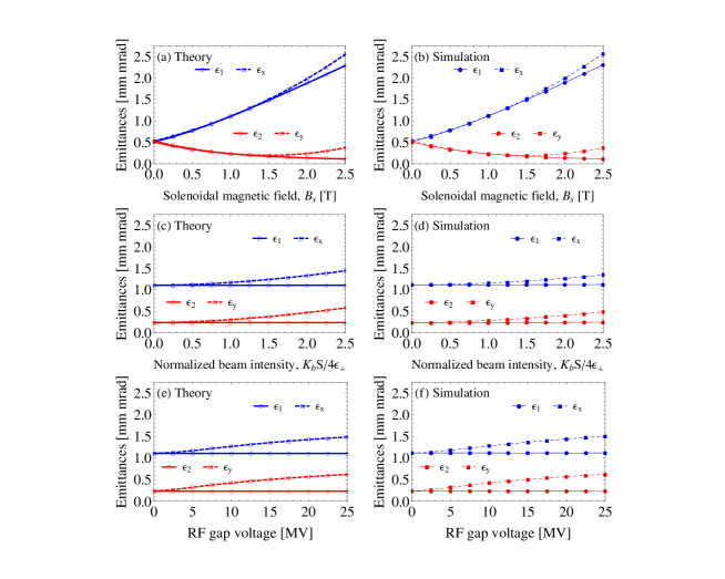
Figure 1: Plots of the eigen-emittances (solid lines with circles) and projected rms emittances (dashed lines with squares) at the exit of the skew-quadrupole triplet. Frames (a), (c), and (e) represent the results of the present KV model analyzed by MATHEMATICA Mat , and frames (b), (d), and (f) represent the results of the multi-particle tracking simulations using TRACK code TRA . Frames (a) and (b) correspond to the cases with $K_{b}=0$ and zero acceleration; frames (c) and (d) to the cases with $B_{s}=1$ T and zero acceleration; frames (e) and (f) to the cases with $B_{s}=1$ T and $K_{b}=0$, respectively.

As a numerical example, we consider an initial beam matrix with parameters of the EMTEX in Ref. Xiao et al. (2013). The focusing coefficients of the skew-quadrupoles are kept fixed at the values used to decouple the beam produced by a solenoidal field of 1.0 T, with the conditions of zero space-charge and zero acceleration. Figures 1(a) and 1(b) indicate that the decoupling processes are not sensitive to the solenoidal field strength $B_{s}$, particulary when $B_{s}\lesssim 1.5$. This tendency has been investigated in detail in Refs. Groening et al. (2014); Groening (2014). Therefore, for a given skew-quadrupole triplet setting, one can obtain arbitrary emittance ratios by simply changing the single parameter $B_{s}$. Figures 1(c) and 1(d) show the effects of the space-charge forces on the decoupling processes. If the normalized beam intensity $K_{b}S/4\epsilon_{\perp}$ (in which $S$ is the axial periodicity length or the characteristic length of the beamline) is greater than about 1.0 (i.e., the space-charge force becomes comparable to or greater than the emittance contribution), the deviations of the rms emittances from the eigen-emittances become significant and increase continuously. Conventional multi-particle tracking simulations including space-charge effects show a good agreement ($<7\%$ of relative errors in projected rms eimttances) with the present KV model. Figures 1(e) and 1(f) show the effects of the beam energy variation on the decoupling processes. The rms emittances deviate from the eigen-emittances when an RF voltage is applied to the acceleration gap located between the solenoid and the skew-quadrupole triplet.

In summary, we have fully generalized the KV model by including all the linear coupling elements, so that it provides a new advanced theoretical tool for the design and analysis of complex beamlines with strong coupling. In the numerical example summarized in Fig. 1, we have demonstrated the usefulness and effectiveness of the new generalized KV model in understanding phase-space manipulations of high-intensity beams, for which previous KV models are inapplicable.