Signatures of bifurcation on quantum correlations: Case of quantum kicked top

Abstract

Quantum correlations reflect the quantumness of a system and are useful resources for quantum information and computational processes. The measures of quantum correlations do not have a classical analog and yet are influenced by the classical dynamics. In this work, by modelling the quantum kicked top as a multi-qubit system, the effect of classical bifurcations on the measures of quantum correlations such as quantum discord, geometric discord, Meyer and Wallach $Q$ measure is studied. The quantum correlation measures change rapidly in the vicinity of a classical bifurcation point. If the classical system is largely chaotic, time averages of the correlation measures are in good agreement with the values obtained by considering the appropriate random matrix ensembles. The quantum correlations scale with the total spin of the system, representing its semiclassical limit. In the vicinity of the trivial fixed points of the kicked top, scaling function decays as a power-law. In the chaotic limit, for large total spin, quantum correlations saturate to a constant, which we obtain analytically, based on random matrix theory, for the $Q$ measure. We also suggest that it can have experimental consequences.

I Introduction

It is well established by more than half a century of quantum chaos research that many of the properties of quantum systems can be understood in terms of classical objects such as periodic orbits and their stability StockmannBook . For classically integrable systems, Einstein-Brillouin-Keller quantization method relates the quantum spectra and the classical action Stone05 while for chaotic systems Gutzwiller’s trace formula represents such an approach connecting the quantum spectra and the classical periodic orbits GutzwillerBook . The advent of quantum information and computation has opened up newer scenarios in which novel quantum correlations did not have corresponding classical analogues. Quantum entanglement is one such phenomena without a classical analogue. The von Neumann entropy, a measure of quantum entanglement for a bipartite pure state, captures correlations with purely quantum origins that are stronger than classical correlations. A host of such measures are now widely used in the quantum information theory to quantify stronger than classical correlations.

Quantum correlations do not have exact classical analogues, yet they are surprisingly affected by the classical dynamics. For instance, in the context of chaotic systems, it is known that upon variation of a parameter, as chaos increases in the system the entanglement also increases and saturates to a value predicted based on random matrix theory Mehtabook . Recently, this was experimentally demonstrated for an isolated quantum system consisting of three superconducting qubits as a realisation of quantum kicked top Neill2016 . It was shown that larger values of entanglement corresponds to regimes of chaotic dynamics arul01 . Theoretically, not just the chaotic dynamics but indeed the structure and details of classical phase space, such as the presence of elliptic islands in a sea of chaos, is known to affect the entanglement Santhanam2008 .

Quantum entanglement is an important resource for quantum information processing and computational tasks. However, it does not capture all the correlations in a quantum system. It is possible for unentangled states to display non-classical behaviour implying that there might be residual quantum correlations beyond what is measured by entanglement. In addition, it is now known that entanglement is not the only ingredient responsible for speed-up in quantum computing Bennett1999 ; Niset2006 ; Horodecki2005 . For mixed state quantum computing model, discrete quantum computation with one qubit (DQC1), experiments have shown that some tasks can be speeded up over their classical counterparts even using non-entangled, i.e., separable states but having non-zero quantum correlations Knill ; Animesh ; laflammeoct11 . Hence, quantification of all possible quantum correlations is important. For this purpose, measures like quantum discord Ollivier ; vedral and geometric discord Dakic ; Luo_geometric , Leggett-Garg inequality LeggettGarg and a host of others are widely used.

Quantum discord is independent of entanglement and no simple ordering relations between them is known Virmani2000 ; ModiRMP . Entanglement may be larger than quantum discord even though for separable states entanglement always vanishes but quantum discord may be nonzero, and thus is less than quantum discord luo ; ARPRau2010 ; ModiRMP . This shows that discord and in general all quantum correlation measures are more fundamental than entanglement Maziero2009 . It is shown that two-qubit quantum discord in a dissipative dynamics under Markovian environments vanishes only in the asymptotic limit where entanglement suddenly disappears Werlang2009 . Thus, the quantum algorithms that make use of quantum correlations, represented in discord, might be more robust than those based on entanglement Werlang2009 . This shows that studying quantum correlation, in general, in a given system is important from the point of view of decoherence which is inevitably present in almost all experimental setups.

In the last decade, many experimental and theoretical studies of discord were performed Celeri2011 . A recent experiment realizes quantum advantage with zero entanglement but with non-zero quantum discord using a single photon’s polarization and its path as two qubits Maldonado2016 . Other experiments have estimated the discord in an anti-ferromagnetic Heisenberg compound Mitra2015 and in Bell-diagonal states Moreva2016 . In the context of chaotic systems, e.g., the quantum kicked top, the dynamics of discord reveals the classical phase space structure VaibhavMadhok2015 . In this paper, we show that period doubling bifurcation ChaosForEngineers in the kicked top leaves its signature in the dynamics of quantum correlation measures such as discord and geometric discord, including the multipartite entanglement measure Meyer and Wallach $Q$ measure Meyer02 .

The structure of the paper is as follows: In Sec. II the measures of quantum correlations used are introduced. In Sec. III the kicked top model is introduced. In Sec. IV results on the effects of the bifurcation on the time averages of these measures of quantum correlations are given. In Sec. V these results are compared with a suitable random matrix model. In Sec. VI scaling of these time averaged measures is studied as a function of total spin.

II Measure of quantum correlations

II.1 Quantum Discord

Quantum discord is a measure of all possible quantum correlations including and beyond entanglement in a quantum state. In this approach one removes the classical correlations from the total correlations of the system. For a bipartite quantum system, its two parts labelled $A$ and $B$, and represented by its density matrix $\rho_{AB}$, if the von Neumann entropy is ${\mathcal{H}}(\rho_{AB})=-\mbox{Tr}~{}(\rho_{AB}\log\rho_{AB})$, then the total correlations is quantified by the quantum mutual information as,

$${\mathcal{I}}(B:A) = {\mathcal{H}}(B)+{\mathcal{H}}(A)-{\mathcal{H}}(B,A).$$ (1)

In classical information theory, the mutual information based on Baye’s rule is given by

$$I(B:A) = H(B)-H(B|A)$$ (2)

where $H(B)$ is the Shannon entropy of $B$. The conditional entropy $H(B|A)$ is the average of the Shannon entropies of system $B$ conditioned on the values of $A$. It can be interpreted as the ignorance of $B$ given the information about $A$.

Quantum measurements on subsystem $A$ are represented by a positive-operator valued measure (POVM) set $\{\Pi_{i}\}$, such that the conditioned state of $B$ given outcome $i$ is

$$\rho_{B|i}=\mbox{Tr}_{A}(\Pi_{i}\rho_{AB})/p_{i}\;\;\mbox{and}\;\;p_{i}=\mbox{Tr}_{A,B}(\Pi_{i}\rho_{AB})$$ (3)

and its entropy is $\tilde{\mathcal{H}}_{\{\Pi_{i}\}}(B|A)=\sum_{i}p_{i}{\mathcal{H}}(\rho_{B|i})$. In this case, the quantum mutual information is ${\mathcal{J}}_{\{\Pi_{i}\}}(B:A)={\mathcal{H}}(B)-\tilde{\mathcal{H}}_{\{\Pi_{i}\}}(B|A)$. Maximizing this over the measurement sets $\{\Pi_{i}\}$ we get

$${\mathcal{J}}(B:A) = \mbox{max}_{\{\Pi_{i}\}}\left({\mathcal{H}}(B)-\tilde{\mathcal{H}}_{\{\Pi_{i}\}}(B|A)\right)$$ (4)

$$= {\mathcal{H}}(B)-\tilde{\mathcal{H}}(B|A)$$

where $\tilde{\mathcal{H}}(B|A)=\mbox{min}_{\{\Pi_{i}\}}\tilde{\mathcal{H}}_{\{\Pi_{i}\}}(B|A)$. The minimum value is achieved using rank $1$ POVMs since the conditional entropy is concave over the set of convex POVMs animesh_nullity . By taking $\{\Pi_{i}\}$ as rank-1 POVMs, quantum discord is defined as ${\mathcal{D}}(B:A)={\mathcal{I}}(B:A)-{\mathcal{J}}(B:A)$, such that

$${\mathcal{D}}(B:A)={\mathcal{H}}(A)-{\mathcal{H}}(B,A)+\mbox{min}_{\{\Pi_{i}\}}\tilde{\mathcal{H}}_{\{\Pi_{i}\}}(B|A).$$ (5)

Quantum discord is non-negative for all quantum states ZurekQuantumDiscord2000 ; Ollivier ; animesh_nullity , and is subadditive VaibhavMadhok11 .

II.2 Geometric Discord

The calculation of discord involves the maximization of $J(A:B)$ by doing measurements on the subsystem $B$, which is a hard problem. A more easily computable form is geometric discord based on a geometric way Dakic ; Luo_geometric . There are no measurements involved in calculating this measure. For the special case of two-qubits a closed form expression is given Dakic . Dynamics of geometric discord is studied under a common dissipating environment Huang2016 . For every quantum state there is a set of postmeasurement classical states, and the geometric discord is defined as the distance between the quantum state and the nearest classical state,

$$D^{G}(B|A)=\min_{\chi\in\Omega_{0}}\|\rho-\chi\|^{2}~{},$$ (6)

where $\Omega_{0}$ represents the set of classical states, and $\|X-Y\|^{2}={\rm Tr}[(X-Y)^{2}]$ is the Hilbert-Schmidt quadratic norm. Obviously, $D^{G}(B|A)$ is invariant under local unitary transformations. Explicit and tight lower bound on the geometric discord for an arbitrary state of a bipartite quantum system $A_{m\times m}\otimes B_{n\times n}$ is available Luo_geometric ; Hassan ; Rana . Recently discovered ways to calculate lower bounds on discord for such general states do not require tomography and, hence, are experimentally realisable Rana ; Hassan .

Following the formalism of Dakic et al. Dakic analytical expression for the geometric discord for two-qubit states is obtained. The two-qubit density matrix in the Bloch representation is

$$\rho=\frac{1}{4}\Big{(}\mathbbm{1}\otimes\mathbbm{1}+\sum_{i=1}^{3}x_{i}\sigma_{i}\otimes\mathbbm{1}+\sum_{i=1}^{3}y_{i}\mathbbm{1}\otimes\sigma_{i}+\sum_{i,j=1}^{3}T_{ij}\sigma_{i}\otimes\sigma_{j}\Big{)}$$ (7)

where $x_{i}$ and $y_{i}$ represent the Bloch vectors for the two qubits, and $T_{ij}={\rm Tr}[\rho(\sigma_{i}\otimes\sigma_{j})]$ are the components of the correlation matrix. The geometric discord for such a state is

$$D^{G}(B|A)=\frac{1}{4}\left(\|x\|^{2}+\|T\|^{2}-\eta_{\rm max}\right),$$ (8)

where $\|T\|^{2}={\rm Tr}[T^{T}T]$, and $\eta_{\rm max}$ is the largest eigenvalue of $\vec{x}\vec{x}^{T}+TT^{T}$, whose explicit form is in Girolami2012 .

II.3 Meyer and Wallach $Q$ measure

In this work, the effects of bifurcation on multipartite entanglement is also studied using the Meyer and Wallach $Q$ measure Meyer02 . This was used to study the multipartite entanglement in spin Hamiltonians ArulLakshminarayan2005 ; Karthik07 ; Brown08 and system of spin-boson Lambert2005 . The geometric multipartite entanglement measure $Q$ is shown to be simply related to one-qubit purities Brennen . Making its calculation and interpretation is straightforward. If $\rho_{i}$ is the reduced density matrix of the $i$th spin obtained by tracing out the rest of the spins in a $N$ qubit pure state then

$$Q(\psi)=2\left(1-\frac{1}{N}\sum_{i=1}^{N}\mbox{Tr}(\rho_{i}^{2})\right).$$ (9)

This relation between $Q$ and the single spin reduced density matrix purities has led to a generalization of this measure to multiqudit states and for various other bipartite splits of the chain Scott2004 .

III kicked top

The quantum kicked top is characterized by an angular momentum vector ${\bf J}=(J_{x},J_{y},J_{z})$, whose components obey the standard angular momentum algebra. Here, the Planck’s constant is set to unity. The dynamics of the top is governed by the Hamiltonian Haakebook :

$$H(t)=pJ_{y}+\frac{k}{2j}J_{z}^{2}\sum_{n=-\infty}^{+\infty}\delta(t-n).$$ (10)

The first term represents the free precession of the top around $y-$axis with angular frequency $p$, and the second term is periodic $\delta$-kicks applied to the top. Each kick results in a torsion about the $z-$axis by an angle $(k/2j)~{}J_{z}$. The classical limit of Eq. (10) is integrable for $k=0$ and becomes increasingly chaotic for $k>0$. The period-1 Floquet operator corresponding to Hamiltonian in Eq. (10) is given by

$$U=\exp\left(-i\frac{k}{2j}J_{z}^{2}\right)\exp\left(-ipJ_{y}\right).$$ (11)

The dimension of the Hilbert space is $2j+1$ so that dynamics can be explored without truncating the Hilbert space. Kicked top was realized in experiments Chaudhury09 and the range of parameters used in this work makes it experimentally feasible.

The quantum kicked top for given angular momentum $j$ can be regarded as a quantum simulation of a collection of $N=2j$ qubits (spin-half particles) whose evolution is restricted to the symmetric subspace under the exchange of particles. The state vector is restricted to a symmetric subspace spanned by the basis states $\{|j,m\rangle;(m=-j,-j+1,...,j)\}$ where $j=N/2$. It is thus a multiqubit system whose collective behavior is governed by the Hamiltonian in Eq. 10 and quantum correlations between any two qubits can be studied. Kicked top has served as a useful model to study entanglement Lombardi2011 ; ShohiniGhose2008 ; Miller99 ; arul01 ; bandyo03 ; BandyoArulPRE and its relation to classical dynamics Ghikas2007 .

The classical phase space shown in Fig. 1 is a function of coordinates $\theta$ and $\phi$. In order to explore quantum dynamics in kicked top, we construct spin-coherent states Hakke87 ; Arecchi1972 ; Glauber1976 ; PuriBook pointing along the direction of $\theta_{0}$ and $\phi_{0}$ and evolve it under the action of Floquet operator. The quantum correlations reported in this paper represent time averages obtained from time evolved spin-coherent state.

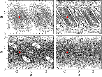
Figure 1: (Color online) Phase-space pictures of the classical kicked top for $p=\pi/2$ and (a) $k=1$, (b) $k=2$, (c) $k=3$ and (d) $k=6$. Red solid circles indicates initial position of the spin coherent state.

The classical map for the kicked top is Haakebook ; Hakke87 ,

$$X^{\prime} = (X\cos p+z\sin p)\cos\left(k\left(z\cos p-X\sin p\right)\right)$$ (12a)

$$-Y\sin\left(k\left(z\cos p-X\sin p\right)\right)$$

$$Y^{\prime} = (X\cos p+Z\sin p)\sin\left(k\left(Z\cos p-X\sin p\right)\right)$$ (12b)

$$+Y\cos\left(k\left(Z\cos p-X\sin p\right)\right)$$

$$Z^{\prime} = -X\sin p+Z\cos p.$$ (12c)

Since the dynamical variables $(X,Y,Z)$ are restricted to the unit sphere i.e. $X^{2}+Y^{2}+Z^{2}=1$, they can be parameterized in terms of the polar angle $\theta$ and the azimuthal angle $\phi$ as $X=\sin\theta\cos\phi$, $Y=\sin\theta\sin\phi$ and $Z=\cos\theta$. We evolve the map in Eq. (12) and determine the values of $(\theta,\phi)$ using the inverse relations (not shown here). For $p=\pi/2$ additional symmetry properties leads to a simpler classical map, a case studied in detail in ref. BandyoArulPRE ; VaibhavMadhok2015 . In this paper two cases namely $p=\pi/2$ and $p=1.7$ are studied which are different from random matrix theory point of view as explained in Sec. V.

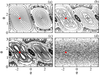
Figure 2: (Color online) Phase-space of the classical kicked top for $p=1.7$ and (a) $k=1$, (b) $k=1.9$, (c) $k=2.1$ and (d) $k=6$. Red solid circles indicates initial position of the spin coherent state.

IV Effect of Bifurcation

Firstly, we consider the case of $p=\pi/2$. If kick strength is $k=1$, then the phase space is largely dominated by invariant tori as seen in Fig. 1(a). In particular, the trivial fixed points of the map at $(\theta,\phi)=(\pi/2,\pm\pi/2)$ visible in Figs. 1(a,b) become unstable at $k=2$. As $k$ increases further, the new fixed points born at $k=2$ move away (see Fig. 1(c)). For $k=6$, the phase space is largely chaotic with no islands visible in 1(d)). In kicked top, the period doubling bifurcation is the route for regular to chaotic transition.

Second case that is studied here is $p=1.7$. As seen in Fig. 2(a-d), the phase space displays similar features as in the case of $p=\pi/2$ except that the trivial fixed point $(\theta,\phi)=(\pi/2,-\pi/2)$ now loses stability at numerically determined $k=1.76$ while $(\theta,\phi)=(\pi/2,\pi/2)$ loses at $k=2.2$. The dark circle, marking the point $(\theta_{0},\phi_{0})=(\pi/2,-\pi/2)$ in Figs. 1 and 2, is the initial position of the spin-coherent state wavepacket.

To study the effect of bifurcation on the quantum correlation and multipartite entanglement measures, multiqubit representation of the system is used. For particular value of $j$ the system can be decomposed into $N=2j$ qubits. The reduced density matrix of two qubits is calculated by tracing out all other $N-2$ qubits WangMolmer2002 ; HuMing2008 after every application of the Floquet map. We use the reduced density matrix to compute the various measures of correlation. As all the qubits are identical, the correlations measures do not depend on the actual choice of two qubits. Similarly, while calculating $Q$ measure one needs to compute reduced density matrix of only one qubit.

The spin-coherent state at time $t=0$ denoted as $|\psi(0)\rangle$ is placed at the fixed point $(\theta,\phi)=(\pi/2,-\pi/2)$ (red solid circle in Figs. 1 and 2) undergoing a period doubling bifurcation. The state $|\psi(0)\rangle$ is evolved by the Floquet operator $\hat{U}$ as $|\psi(n)\rangle=U^{n}|\psi(0)\rangle$. We apply the numerical iteration scheme given in refs. Miller99 ; AsherPeres1996 for time evolving the initial state. At every time step, discord $D$, geometric discord $D^{G}$ and, Meyer and Wallach $Q$ measure is calculated for given value of $k$. The results shown in Figs. 3 and 4 represent time averaged values of $D$, $D^{G}$ and $Q$ for every $k$.

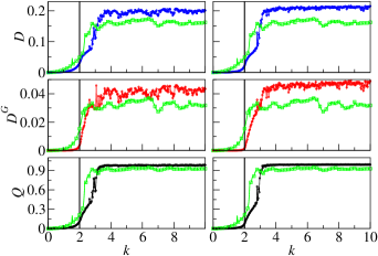
Figure 3: (Color online) Average discord, geometric discord and $Q$ measure as a function of $k$ for $p=\pi/2$. Left (right) column is for $j=50$ ($j=120$). For comparison purposes, $j=10$ case is shown in every graph as square (green) symbols. The vertical line marks the position of bifurcation at $k=2$.

For both cases of $p=\pi/2$ (Fig. 3) and $p=1.7$ (Fig. 4), the results are shown for two different values of $j$, namely, $j=50$ and $j=120$. For comparison, the case of $j=10$ qubits is also shown in Fig. 3. Broadly, in all the cases, the quantum correlation measures $D$, $D^{G}$ and $Q$ respond to the classical bifurcation in a similar manner; by displaying a jump in the mean value from about 0 to a non-zero value. This can be understood as follows. When the elliptic islands are large, as is the case when $0<k<2$ for $p=\pi/2$ and $0<k<1.76$ for $p=1.7$ case, the evolution of the spin-coherent state placed initially at $(\theta,\phi)=(\pi/2,-\pi/2)$ is largely confined to the same elliptic islands. As the bifurcation point is approached, the local instability in the vicinity of the fixed point evolves part of the coherent state into the chaotic layers of phase space. This leads to an increase in the values of correlation measures. Note that increasing chaos leads to an increase in entanglement too. When $j$ is increased, the width of coherent state $\sigma\propto 1/\sqrt{j}$ becomes narrower and closely mimics the classical evolution Hakke87 . Thus, as $j$ increases, we expect the quantum correlations to sharply respond to classical bifurcation at $k=2$. Indeed, as seen in Fig. 3, the quantum correlations changes sharply at $k=2$ for $=120$ in comparison with the case of $j=10$. To understand the details of Fig. 3 consider two values of $j$, e.g., $j=j_{1}$ and $j=j_{2}$ such that $j_{2}>j_{1}$. The slow decay of $\sigma$ as $j\to\infty$ implies that the response of quantum correlations to classical bifurcation becomes perceptible only when $|j_{2}-j_{1}|>>1$. Thus, relative changes are easily seen when quantum correlations for $j=120$ is compared with $j=10$ case rather than with that of $j=50$. The approach to semiclassics, $\hbar\to 0$ limit, discussed in Section VI provides a quantitative support to this picture.

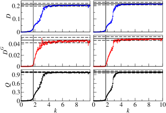
Figure 4: (Color online) Average discord, geometric discord and $Q$ measure as a function of $k$ for $p=1.7$. Left (right) column is for $j=50$ ($j=120$). The solid horizontal line represents the long time average of an initial state from the bifurcation point evolved using the operator $U_{CUE}$. The dashed line represent the standard deviation from the average value. Vertical line marks the position of bifurcation approximately at $k=1.76$.

V Correlation measures and random matrix theory

Next, we show that the saturated values for $D$, $D^{G}$ and $Q$ after bifurcation has taken place at $k=k_{b}$, can be obtained from random matrix considerations. The kicked top is time-reversal invariant and as a consequence its Floquet operator in the globally chaotic case has the statistical properties of a random matrix chosen from the circular orthogonal ensemble (COE) Kus1988 . For kicked top, the statistical properties of eigenvectors of its Floquet operator are in good agreement with COE of random matrix theory Kus1988 . Apart from time-reversal symmetry, the kicked top additionally has the parity symmetry, $\widehat{R}_{y}=\mbox{exp}(-i\pi j_{y})$ that commutes with the Floquet operator for all values of $p$. As $\widehat{R}_{y}^{2}=I$, the eigenvalues of $\widehat{R}_{y}$ are $+1$ and $-1$. Thus, in the basis of the parity operator, the Floquet operator has a block-diagonal structure consisting of two blocks associated with the positive-($+1$) or negative-parity ($-1$) eigenvalues. Thus, due to the parity symmetry, the kicked top is statistically equivalent to a block-diagonal random matrix (block diagonal in the basis in which the parity operator is diagonal) whose blocks (corresponding to the eigenvalues $\pm 1$) are sampled from the COE Mehtabook . If $p=\pi/2$ the kicked top posseses additional symmetries Kus1988 , the case which is not considered in this section. In this section, the case when $p=1.7$ is studied in detail.

Firstly, a block-diagonal COE as the appropriate ensemble of random matrices for modeling the kicked-top Hamiltonian is used. Since the basis here is that of eigenvectors of the parity operator $\widehat{R}_{y}$, this matrix is then written in the $|j,m\rangle$ basis. Finally, this matrix is used to evolve the coherent state and compared with the evolution done using the Floquet operator in the globally chaotic case ($k=10$). The results are presented in Fig. 5 and summarised in Table 1.

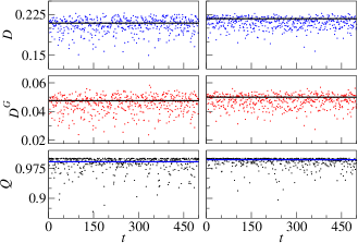
Figure 5: (Color online) Time variation of the correlation measures using kicked-top Floquet operator for $j=50$ (left) and for $j=120$ (right) for the globally chaotic case ($k=10$ and $p=1.7$). Horizontal line corresponds to time average of the correlation measures using a COE matrix of the respective case.

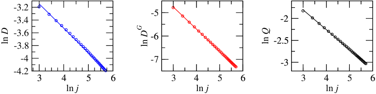
Figure 6: (Color online) The variation of time-averaged quantum correlations (circles) as a function of $j$. The lines are the power law fits given in Eq. (13).

Fig. 5 shows the evolution of $2$-qubit discord, geometric discord and Meyer-Wallach $Q$ measure for $j=50$ and $j=120$ when acted by kicked-top Floquet operator with $k=10$. At this kick strength the classical phase space of kicked top is largely chaotic with no visible regular regions. As Fig. 5 and Table 1 reveal, the dynamics of various correlations measures under the action of COE matrix is similar to that of kicked-top Floquet operator in its chaotic regime with $k=10$. While this is not entirely unexpected, the values of the three measures listed in Table 1 closely agree with those obtained after bifurcation takes place at $k=k_{b}$, but at values of kick strengths much less than $10$ considered in Fig. 5. Time averages listed in Table 1 are plotted in Fig. 4 along with the standard deviation of the individual measures. It can be seen that the agreement between these values and that of Floquet operator begins to emerge at around $k=4$ which is much less than $k=10$. The position of the coherent state in this case is $(\theta,\phi)=(\pi/2,-\pi/2)$. It should be noted that in the globally chaotic case these results are independent of the initial position of the coherent state.

It can be seen from Table 1 and Fig. 4 that the time averages of quantum correlations for the kicked top are systematically, although slightly, lower than that predicted by the circular orthogonal ensemble (COE) of random matrix theory. The agreement improves as $j\to\infty$. Hence, these deviations can be attributed to finite $j$ effect. Similar systematic deviations from RMT were observed in the study of the log-negativity in kicked rotor system Uday12 . In this case too, the deviations decreased as the corresponding Hilbert space dimensions were increased.

	$j=50$	$j=50$	$j=120$	$j=120$
Measure	Floquet	COE	Floquet	COE
Discord	$0.205$	$0.209$	$0.217$	$0.217$
Geometric discord	$0.045$	$0.047$	$0.049$	$0.050$
$Q$ measure	$0.986$	$0.991$	$0.994$	$0.996$

Table 1: Mean value of correlation measures averaged over $1000$ time steps of evolution of a coherent state with the Floquet matrix (with $k=10$) and the COE matrix. The COE values are represented in Fig. 4 as horizontal lines.

VI Scaling with Planck volume

Kicked top is a finite dimensional quantum system and the volume of its Planck cell is $V=4\pi/(2j+1)$. For large $j$, $V\propto 1/j$. It is natural to ask how the measures of quantum correlation scale with this volume when kick strength corresponds to $k=k_{b}$ where $k_{b}$ is a bifurcation point. In Fig. 6, we show the variation in the time average of $D$, $D^{G}$ and $Q$ as a function of $j$ for $k=k_{b}$. Here, $k_{b}=2$ and $p=\pi/2$. The coherent state is placed at the corresponding trivial fixed point $(\theta,\phi)=(\pi/2,-\pi/2)$ and the time average is taken over $500$ steps. For  $j>>1$, the correlation measures scale with $j$ approximately in a power-law of the form $j^{-\mu}$, $\mu$ is the scaling exponent. The power law fits through linear regression for the numerically computed correlations measures shown in Fig. 6 are consistent with

$$D\propto j^{-\mu_{1}},\;\;\;D^{G}\propto j^{-\mu_{2}}\;\;\;\mbox{and}\;\;\;Q\propto j^{-\mu_{3}},$$ (13)

where $\mu_{1}=0.382\pm 0.003$, $\mu_{2}=0.944$ and $\mu_{3}=0.451$. The uncertainty values are estimated by numerical linear regression The uncertainties in the estimates for $\mu_{2}$ and $\mu_{3}$ are of the order of $10^{-8}$ and hence negligible. Identical power-law scaling is obtained for the other trivial fixed point at $(\theta,\phi)=(\pi/2,\pi/2)$ with exponents $\mu_{i}$ approximately same as given in Eq. (13). The quantum correlations tend to zero as $V\to 0$ ($j\to\infty$) indicating that for any finite $j$ quantum correlations, however small it might be, would continue to exist. As the wavepacket becomes more ’classical’ and the underlying dynamics is regular, we expect the quantum correlations to decrease with $j$. This is another indication that the regular regions in the vicinity of the fixed point undergoing bifurcations affect the quantum correlations deep in the semiclassical regime.

The appearance of power-law scaling can be understood for the case $k=2$ when the regular region is large and the chaotic layer is a tiny fraction of the entire phase space. The presence of chaotic layer has a strong influence on quantum correlations. Note that for $j>>1$, the width of the spin-coherent state $\sigma=j^{-1/2}$ becomes small and its evolution is mostly confined to the large elliptic islands in Fig. 1(a,b). As a result, it can be argued that the strength of the overlap of coherent state with the chaotic layer is indicative of quantum correlations. Since $\sigma=j^{-1/2}$, for $j>>1$, this overlap is small. The slow power-law decay of $\sigma$ might possibly be the reason for similar decay of quantum correlations as well, as shown in Eq. (13). Since quantum correlations are affected by the local phase space features, a complete quantitative explanation for power-law scaling might require a detailed semiclassical analysis.

Next, we consider the case of a coherent state placed initially at a bifurcation point leading to a period-2 cycle. The origin of this bifurcation point is as follows. The trivial fixed points at $(\theta,\phi)=(\pi/2,\pm\pi/2)$ are easily visible in Figs. 1(a-b) and 2(a-b). If $p=\pi/2$, these fixed points bifurcate at $k=2$ through a period doubling bifurcation and become unstable. In the process, the point $(\theta,\phi)=(\pi/2,\pi/2)$ gives rise to two new period-$1$ stable fixed points while the point $(\theta,\phi)=(\pi/2,-\pi/2)$ gives rise to a period-2 cycle. For $k>2$ their positions move in the phase space as a function of $k$ and they are stable for $k\leq\sqrt{2}\pi$. For $k>\sqrt{2}\pi$, the two fixed points bifurcate into two new period-2 cycles while the period-2 cycle gives rise to a new period-4 cycle. Their positions for $k=\sqrt{2}\pi$ are shown in Fig. 7. Our interest lies in the fixed point located at $(\theta,\phi)=(\pi/4,0)$.

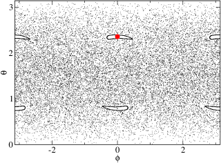
Figure 7: (Color online) Phase-space picture of the classical kicked top for $k=\sqrt{2}\pi$. Red solid circles indicates initial position of the spin coherent state.

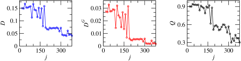
Figure 8: (Color online) The variation of time-averaged quantum correlations (circles connected with lines) as a function of $j$ for $k=\sqrt{2}\pi$ and initial position of the spin coherent state as shown in Fig. 7.

Fig. 8 shows variation of the time average of the quantum correlation measures as a function of $j$ for the initial coherent state placed at this fixed point. It can be seen that after initial fluctuations the correlations start to decrease for larger values of $j$. It should be noted that the area of elliptic islands are continually shrinking as $k\to\infty$ consistent with the predominance of chaotic regions in the phase space. The width of the spin-coherent state $|\psi(0)\rangle$ is equal to $1/\sqrt{j}$. For small values of $j$, the width of $|\psi(0)\rangle$ is much larger than that of the regular elliptic island as shown in Fig. 7. Hence, there is a pronounced overlap of the state $|\psi(0)\rangle$ with the chaotic sea. Hence we expect that for small $j$ the quantum correlations will be reasonably close to their random matrix averages. This is indeed seen in Figs. 8 for $1\leq j\leq 50$ as the width of $|\psi(0)\rangle$ are at least twice the size of elliptic island. For $j>>1$, the width of $|\psi(0)\rangle$ has become much smaller than that of elliptic island. Thus, under these conditions we expect smooth decay with increasing $j$, similar to what is seen in Fig. 6(a-c). Fig. 8 do show smooth decay for $j\gtrsim 150$. Thus, the quantum correlations, on an average, decay as a function of $j$ and the area of the regular region surrounding the fixed point undergoing bifurcation strongly affects the quantum correlations.

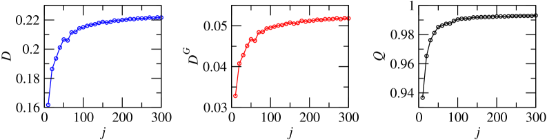
Figure 9: (Color online)The variation of time-averaged quantum correlations (circles) as a function of $j$ for the globally chaotic case ($k=10$)..

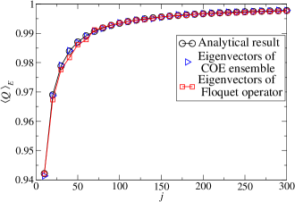
Figure 10: (Color online) Average $Q$ measure for the eigenvectors of COE ensemble and that of Floquet operator in the globally chaotic case for the parameter range $10\leq k\leq 1000$ and $p=1.7$ are compared with its analytical expression given in Eq. (14).

Now, we consider kick strength $k=10$ and place the spin-coherent state $|\psi(0)\rangle$ at an arbitrary position in the chaotic sea, namely, $(\theta,\phi)=(1.6707,−1.3707)$. Here, the phase space is largely chaotic devoid of any regular regions. In contrast to the results in Figs. 6 and 8, the time averaged correlation measures shown in Fig. 9 increase with $j$. Based on the results from figs. 4 and 5 we can expect that at every value of $j$ the time averaged $D$, $D_{G}$ and $Q$ agree with those found using apropriate COE ensemble.

For a coherent state the quantum correlation measures are zero. However, after time evolution, the correlation values will depend on the corresponding measures for Floquet eigenstates. Thus, it is important to study the typical values of these measures for these eigenstates. This can be analytically obtained for the average $Q$ measure. An exact analytical formula for the average $Q$ measure is derived (see Appendix A for the detailed derivation) for a typical COE ensemble modelling the Floquet operator in the globally chaotic case. It is given by

$$\langle Q\rangle_{E}=1-\frac{16j(j+1)}{3(2j+3)(2j+1)^{2}}.$$ (14)

For large $j$, $\langle Q\rangle_{E}\approx 1-2/(3j)$ implying that the measure tends to one for large $j$. The numerically computed correlations for the eigenvectors of COE ensemble and for the eigenvectors of the Floquet operator under conditions of globally classical chaos are compared with the analytical result in Eq. (14) in Fig. 10.

For generating sufficient statistics for the eigenvectors of Floquet operator, we use a range of $k$ values such that the corresponding classical section does not have any significant regular islands and is highly chaotic. The analytical result in Eq. (14) agrees with that for the eigenvectors of the COE ensemble. In order to derive similar expressions for the average discord and geometric discord for the eigenvectors of COE, analytical expression for the distribution of the matrix elements of the two-qubit density matrix for these class of states is required. Such an expression is not known yet, to the best of our knowledge. Thus, the derivation of the average discord and geometric discord as a function of $j$ remains an open question.

It is instructive to compare these results with other well-studied ensembles such as the Gaussian ensembles. In this case, the states are distributed uniformly, also known as Haar measure, on the unit sphere. Consider a tripartite random pure state. The entanglement between any of its two subsystems shows a transition from being entangled to separable state as the size of the third subsystem is increased Uday12 ; Scott03 . Another example is that of definite particle states. This shows algebraic to exponential decay of entanglement when the number of particles exceed the size of two subsystems Vikram11 . For both these cases, discord and geometric discord between two qubits in a tripartite system goes to zero as the size of the third subsystem is increased. It is known that average $Q$ measure for Haar distributed states of $N$ qubits, for large $N$, goes as $1-3/2^{N}$ Scott03 . In terms of $j(=N/2)$ it equals $1-3/2^{2j}$ implying that the measure tend to $1$ for large $j$. But, the rate at which it approaches $1$ is much faster than that for eigenvectors of COE ensemble corresponding to the kicked top in globally chaotic case. In contrast to the standard Gaussian or circular ensemble, the random matrix ensemble appropriate for the kicked top is COE with additional particle exchange symmetry. Hence, this ensemble displays different properties from the standard circular or Gaussian ensembles as far as the quantum correlations are concerned.

Interestingly, it is found numerically in the globally chaotic case that $D^{G}=0.317~{}D-0.018$ holds good. This is seen in Figs. 3, 4, 5 and 9. Such simple relation relating $Q$ measure and discord or geometric discord could not be discerned. It is known that for two-qubit states, discord and geometric discord are related to each other by $D^{G}\geq D^{2}/2$ Luo_geometric ; girolami ; ModiRMP . This inequality is respected thoughout numerical simulations performed here.

VII Summary and Conclusions

In this paper, we have investigated the effect of classical bifurcations on the measures of quantum correlations such as quantum discord, geometric discord and Meyer and Wallach $Q$ measure using kicked top as a model of quantum chaotic system. In a related work VaibhavMadhok2015 , signature of classical chaos in the kicked top was found in the dynamics of quantum discord and this work explores this relation in the more general context of quantum correlations including multipartite entanglement. The suitability of kicked top is due to the fact that it can be represented as a collection of qubits. Most importantly, this system has been realised in experiments Chaudhury09 . A prominent feature in its phase space is the period-1 fixed point whose bifurcation is associated with the quantum discord climbing from nearly $0$ to a value that is in agreement with the numerically determined random matrix equivalent. The transition in the quantum discord reflects the qualitative change in the classical phase space; from being dominated by elliptic island to a largely chaotic sea with a few small elliptic islands. The other measures we have reported here, namely the geometric discord and Meyer and Wallach $Q$ measure, both display similar trends as the quantum discord. Other measures of quantum correlations can be expected to display qualitatively similar results. We have also presented numerical results for the random matrix averages of these quantum correlation measures.

In general, as a function of chaos parameter, quantum discord can be expected to increase under the influence of a period-doubling bifurcation. However, after the bifurcation has taken place, the saturation to the random matrix average will depend on the qualitative nature of dynamics in the larger neighbourhood around the fixed point. It must also be pointed out that these results have been obtained through time evolution of a spin-coherent state placed initially on an elliptic island undergoing bifurcation. For reasonably large elliptic islands, equivalent results could have been obtained by considering the Floquet states of the kicked top as well.

We have also investigated the fate of quantum correlations in the semiclassical limit as Planck volume tends to zero. In the context of kicked top, this limit translates as $j\to\infty$. In the case of bifurcation associated with larger islands, as in $k\leq 2$, the measures of quantum correlations decreases as a function of $j$ and tends to $0$ through a slow, approximately power-law decay. In the case of bifurcation associated with smaller islands and creation of higher order periodic cycles the average decay of quantum correlations is evident but marked by strong fluctuations. The quantum correlation measures reported here have been obtained as that for the time average of an evolving spin-coherent state placed initially at a chosen position in phase space. However, we note that if the spin-coherent state is placed instead in the chaotic sea initially, then a different behaviour is obtained. As a function of $j$, in this case, the quantum correlation measures increases and saturates to a constant value that can be understood based on eigenvectors of appropriate random matrix ensemble. Evaluation of exact analytical expression for average $Q$ measure for the eigenvectors of the corresponding circular unitary ensemble is carried out and agrees very well that for the eigenvectors of the Floquet operator in the globally chaotic case.

All the results presented in this work emphasise the special role played by the bifurcations and the associated regular phase space regions in modifying general expectations for the quantum correlations based on random matrix equivalents. These results are important from the experimental point of view as the kicked top was first implemented in a system of laser cooled Caesium atoms Chaudhury09 . Recently this model was implemented using superconducting qubits Neill2016 . Here the time-averaged von Neumann entropy has shown very close resembalance, despite presence of the decoherence, with the corresponding classical phase-space structure for given parameter values Neill2016 . Hence, the detailed effects of bifurcations presented here should be amenable to experiments as well. The scaling of quantum correlations with the total spin should also be observable with less than about ten superconducting qubits.

Appendix A Exact evaluation of $\langle Q\rangle_{E}$

In this Appendix an exact evaluation of the ensemble average of the Meyer and Wallach $Q$ measure is calculated. The states in the ensemble have idetical qubits and remains unchanged under qubit exchange. As explained in Section III one needs to use symmetric subspace spanned by the basis states $\{|j,m\rangle;(m=-j,-j+1,...,j)\}$. Any pure state $|\phi\rangle$ in this basis is given as

$$|\phi\rangle=\sum_{m=-j}^{j}a_{m}|j,m\rangle\;\;\mbox{where}\;\;\sum_{m=-j}^{j}|a_{m}|^{2}=1.$$ (15)

In this case the $Q$ measure is given as follows:

$$Q=1-\frac{4}{(2j+1)^{2}}\left(\langle S_{z}\rangle^{2}+\langle S_{+}\rangle\langle S_{-}\rangle\right)$$ (16)

where $S_{z}$ and $S_{\pm}$ are collective spin operators such that $S_{z}|j,m\rangle=m|j,m\rangle$ and $S_{\pm}|j,m\rangle=\sqrt{(j\mp m)(j\pm m+1)}|j,m\pm 1\rangle$ HuMing2008 . The ensemble average is carried over the states such that they have the statistical properties of the eigenvectors of the COE ensemble. For the state $|\phi\rangle$ one obtains the following expression for the expectation:

$$\langle S_{z}\rangle=\sum_{m=-j}^{j}m|a_{m}|^{2}.$$ (17)

This gives

$$\langle S_{z}\rangle^{2} = \sum_{m,n=-j}^{j}mn|a_{m}|^{2}|a_{n}|^{2}$$ (18)

$$= \sum_{m=n}m^{2}|a_{m}|^{4}+\sum_{m\neq n}mn|a_{m}|^{2}|a_{n}|^{2}.$$

Now, an exact RMT ensemble-average is carried out Ullah ; Haakebook . Firstly, one obtains

$$\langle\langle S_{z}\rangle^{2}\rangle_{E}=\sum_{m=n}m^{2}\langle|a_{m}|^{4}\rangle_{E}+\sum_{m\neq n}mn\langle|a_{m}|^{2}|a_{n}|^{2}\rangle_{E}.$$ (19)

It should be noted that the first expectation is for a given state $|\phi\rangle$ and second expectation with subscript $E$ denotes the ensemble average over all $|\phi\rangle$ having statistical properties of COE eigenvectors. Using the RMT ensemble averages Ullah ; Haakebook

$$\begin{split}\langle|a_{m}|^{4}\rangle_{E}&=\frac{3}{(2j+1)(2j+3)},\\ \langle|a_{m}|^{2}|a_{n}|^{2}\rangle_{E}&=\frac{1}{(2j+1)(2j+3)}\end{split}$$ (20)

one obtains

$$\begin{split}\langle\langle S_{z}\rangle^{2}\rangle_{E}&=\frac{3}{(2j+1)(2j+3)}\sum_{m=n}m^{2}+\\ &\frac{1}{(2j+1)(2j+3)}\sum_{m\neq n}mn.\end{split}$$ (21)

The first summation in the above equation is calculated as follows:

$$\sum_{m=-j}^{j}m^{2}=2\sum_{m=1}^{j}m^{2}=\frac{j(j+1)(2j+1)}{3}.$$ (22)

The second summation is now calculated. Consider the equality:

$$\left(\sum_{m=-j}^{j}m\right)\left(\sum_{m=-j}^{j}n\right) = 0.$$ (23)

This gives

$$\sum_{m,n}mn=\sum_{m=n}m^{2}+\sum_{m\neq n}mn=0$$ (24)

Thus,

$$\sum_{m\neq n}mn=-\sum_{m=n}m^{2}=\frac{-j(j+1)(2j+1)}{3}.$$ (25)

The ensemble average in Eq. (19) is given as follows:

$$\langle\langle S_{z}\rangle^{2}\rangle_{E}=\frac{2j(j+1)(2j+1)}{3(2j+1)(2j+3)}.$$ (26)

Considering the average of operators $S_{\pm}$ for the state $|\phi\rangle$

$$\langle S_{\pm}\rangle=\sum a_{m}a_{m\pm 1}^{*}\sqrt{(j\mp m)(j\pm m+1)}.$$ (27)

This gives

$$\begin{split}&\langle S_{+}\rangle\langle S_{-}\rangle=\sum_{m,n}a_{m}a_{m+1}^{*}a_{n}a_{n-1}^{*}\\ &\sqrt{(j-m)(j+m+1)(j+n)(j-n+1)}.\end{split}$$ (28)

It can be seen that the ensemble average will have nonzero contribution only when $m=n-1$. Thus,

$$\begin{split}&\langle\langle S_{+}\rangle\langle S_{-}\rangle\rangle_{E}=\\ \sum_{m=-j}^{j-1}&\langle|a_{m}|^{2}|a_{m+1}|^{2}\rangle_{E}(j-m)(j+m+1).\end{split}$$ (29)

Using Eq. (20) following is obtained:

$$\begin{split}&\langle\langle S_{+}\rangle\langle S_{-}\rangle\rangle_{E}=\\ &\frac{1}{(2j+1)(2j+3)}\sum_{m=-j}^{j-1}(j-m)(j+m+1).\end{split}$$ (30)

Calculating the summation as follows:

$$\sum_{m=-j}^{j-1}(j-m)(j+m+1)=\sum_{m=-j}^{j-1}(j^{2}+j-m^{2}-m)$$

$$=2j(j^{2}+j)-\sum_{m=-j}^{j-1}m-\sum_{m=-j}^{j-1}m^{2}$$

$$=2j(j^{2}+j)+j+j^{2}-\frac{j(j+1)(2j+1)}{3}.$$ (31)

Thus,

$$\langle\langle S_{+}\rangle\langle S_{-}\rangle\rangle_{E}=\frac{2j(j+1)}{3(2j+3)}.$$ (32)

Using Eqs. (26) and (32) the final expression for the ensemble average of $Q$ measure, denoted as $\langle Q\rangle_{E}$, is given as follows:

$$\langle Q\rangle_{E}=1-\frac{16j(j+1)}{3(2j+3)(2j+1)^{2}}.$$ (33)

This analytical expression is plotted in Fig. 10.

References

- (1) H.-J. Stöckmann, Quantum Chaos: An Introduction (University Press, Cambridge, 1999)
- (2) A. D. Stone, Physics Today 58, 37 (2005)
- (3) M. C. Gutzwiller, Chaos in Classical and Quantum Mechanics (Springer-Verlag, New York, 1990)
- (4) M. L. Mehta, Random Matrices (Elsevier Academic Press, 3rd Edition, London, 2004)
- (5) C. Neill, P. Roushan, M. Fang, Y. Chen, M. Kolodrubetz, Z. Chen, A. Megrant, R. Barends, B. Campbell, B. Chiaro, et al., Nature Physics(2016)
- (6) A. Lakshminarayan, Phys. Rev. E 64, 036207 (2001)
- (7) M. S. Santhanam, V. B. Sheorey, and A. Lakshminarayan, Phys. Rev. E 77, 026213 (2008)
- (8) C. H. Bennett, D. P. DiVincenzo, C. A. Fuchs, T. Mor, E. Rains, P. W. Shor, J. A. Smolin, and W. K. Wootters, Phys. Rev. A 59, 1070 (1999)
- (9) J. Niset and N. J. Cerf, Phys. Rev. A 74, 052103 (2006)
- (10) M. Horodecki, P. Horodecki, R. Horodecki, J. Oppenheim, A. Sen(De), U. Sen, and B. Synak-Radtke, Phys. Rev. A 71, 062307 (2005)
- (11) E. Knill and R. Laflamme, Phys. Rev. Lett. 81, 5672 (1998)
- (12) A. Datta, A. Shaji, and C. M. Caves, Phys. Rev. Lett. 100, 050502 (2008)
- (13) G. Passante, O. Moussa, D. A. Trottier, and R. Laflamme, Phys. Rev. A 84, 044302 (2011)
- (14) H. Ollivier and W. H. Zurek, Phys. Rev. Lett. 88, 017901 (2001)
- (15) L. Henderson and V. Vedral, J. Phys. A: Math. Gen. 34, 6899 (2001)
- (16) B. Dakić, V. Vedral, and i. c. v. Brukner, Phys. Rev. Lett. 105, 190502 (2010)
- (17) S. Luo and S. Fu, Phys. Rev. A 82, 034302 (2010)
- (18) A. J. Leggett and A. Garg, Phys. Rev. Lett. 54, 857 (1985)
- (19) S. Virmani and M. B. Plenio, Phys. Lett. A 268, 31 (2000)
- (20) K. Modi, A. Brodutch, H. Cable, T. Paterek, and V. Vedral, Rev. Mod. Phys. 84, 1655 (2012)
- (21) S. Luo, Phys. Rev. A 77, 042303 (2008)
- (22) M. Ali, A. R. P. Rau, and G. Alber, Phys. Rev. A 81, 042105 (2010)
- (23) J. Maziero, L. C. Céleri, R. M. Serra, and V. Vedral, Phys. Rev. A 80, 044102 (2009)
- (24) T. Werlang, S. Souza, F. F. Fanchini, and C. J. Villas Boas, Phys. Rev. A 80, 024103 (2009)
- (25) L. C. Celeri, J. Maziero, and R. M. Serra, Int. J. Quant. Inform. 09, 1837 (2011)
- (26) A. Maldonado-Trapp, P. Solano, A. Hu, and C. W. Clark(2016), arXiv:1604.07351 [quant-ph]
- (27) H. Singh, T. Chakraborty, P. K. Panigrahi, and C. Mitra, Quantum Inf Process 14, 951 (2015)
- (28) E. Moreva, M. Gramegna, M. A. Yurischev, and M. Genovese(2016), arXiv:1605.01206v1 [quant-ph]
- (29) V. Madhok, V. Gupta, D.-A. Trottier, and S. Ghose, Phys. Rev. E 91, 032906 (2015)
- (30) T. Kapitaniak, Chaos for Engineers: Theory, Applications, and Control (Springer-Verlag Berlin Heidelberg, 2000) ISBN 978-3-540-66574-8,978-3-642-57143-5
- (31) D. A. Meyer and N. R. Wallach, J. Math. Phys 43, 4273 (2002)
- (32) A. Datta, ph.D. thesis, The University of New Mexico, arXiv:0807.4490; arXiv:1003.5256.
- (33) W. H. Zurek, Ann. Phys. (Berlin) 9, 855 (2000)
- (34) V. Madhok and A. Datta, Phys. Rev. A 83, 032323 (2011)
- (35) Z. Huang and D. Qiu, Quantum Inf. Process. 15, 1979 (2016)
- (36) A. S. M. Hassan, B. Lari, and P. S. Joag, Phys. Rev. A 85, 024302 (2012)
- (37) S. Rana and P. Parashar, Phys. Rev. A 85, 024102 (2012)
- (38) D. Girolami and G. Adesso, Phys. Rev. Lett. 108, 150403 (2012)
- (39) A. Lakshminarayan and V. Subrahmanyam, Phys. Rev. A 71, 062334 (2005)
- (40) J. Karthik, A. Sharma, and A. Lakshminarayan, Phys. Rev. A 75, 022304 (2007)
- (41) W. G. Brown, L. F. Santos, D. J. Starling, and L. Viola, Phys. Rev. E 77, 021106 (2008)
- (42) N. Lambert, C. Emary, and T. Brandes, Phys. Rev. A 71, 053804 (2005)
- (43) G. K. Brennen, Quantum Inf. Comput. 3, 619 (2003)
- (44) A. J. Scott, Phys. Rev. A 69, 052330 (2004)
- (45) F. Haake, Quantum Signatures of Chaos (Springer, 3rd Edition, Berlin, 2010)
- (46) S. Chaudhury, A. Smith, B. E. Anderson, S. Ghose, and P. S. Jessen, Nature 461, 768 (2009)
- (47) M. Lombardi and A. Matzkin, Phys. Rev. E 83, 016207 (2011)
- (48) S. Ghose, R. Stock, P. Jessen, R. Lal, and A. Silberfarb, Phys. Rev. A 78, 042318 (2008)
- (49) P. A. Miller and S. Sarkar, Phys. Rev. E 60, 1542–1550 (1999)
- (50) J. N. Bandyopadhyay and A. Lakshminarayan, Phys. Rev. Lett. 89, 060402 (2002)
- (51) J. N. Bandyopadhyay and A. Lakshminarayan, Phys. Rev. E 69, 016201 (2004)
- (52) G. Stamatiou and D. P. K. Ghikas, Phys. Lett. A 368, 206 (2007)
- (53) F. Haake, M. Kus, and R. Scharf, Z. Phys. B 65, 381 (1987)
- (54) F. T. Arecchi, E. Courtens, R. Gilmore, and H. Thomas, Phys. Rev. A 6, 2211 (1972)
- (55) R. J. Glauber and F. Haake, Phys. Rev. A 13, 357 (1976)
- (56) R. R. Puri, Mathematical Methods of Quantum Optics (Springer, Berlin, 2001)
- (57) X. Wang and K. Mølmer, Euro. Phys. J. D 18, 385 (2002)
- (58) H. Ming-Liang and X. Xiao-Qiang, Chinese Phys. B 17, 3559 (2008)
- (59) A. Peres and D. Terno, Phys. Rev. E 53, 284 (1996)
- (60) M. Kus, J. Mostowski, and F. Haake, J. Phys. A: Math. Gen. 21, L1073 (1988)
- (61) U. T. Bhosale, S. Tomsovic, and A. Lakshminarayan, Phys. Rev. A 85, 062331 (2012)
- (62) A. J. Scott and C. M. Caves, J. Phys. A: Math. Gen. 36, 9553 (2003)
- (63) V. S. Vijayaraghavan, U. T. Bhosale, and A. Lakshminarayan, Phys. Rev. A 84, 032306 (2011)
- (64) D. Girolami and G. Adesso, Phys. Rev. A 83, 052108 (2011)
- (65) N. Ullah and C. E. Porter, Phys. Lett. 6, 301 (1963)