Measuring effective temperatures in a generalized Gibbs ensemble

Abstract

The local physical properties of an isolated quantum statistical system in the stationary state reached long after a quench are generically described by the Gibbs ensemble, which involves only its Hamiltonian and the temperature as a parameter. If the system is instead integrable, additional quantities conserved by the dynamics intervene in the description of the stationary state. The resulting generalized Gibbs ensemble involves a number of temperature-like parameters, the determination of which is practically difficult. Here we argue that in a number of simple models these parameters can be effectively determined by using fluctuation-dissipation relationships between response and correlation functions of natural observables, quantities which are accessible in experiments.

I Introduction

A question of fundamental relevance in the physics of many-body quantum systems is under which conditions and in which sense they can reach an eventual equilibrium state after evolving in isolation from the surrounding environment. With this issue is mind, a considerable theoretical and experimental effort is currently devoted to studying the dynamics of these systems from various perspectives Polkovnikov10 ; Gogolin ; Pasquale-ed .

A statistical system reaches a steady state if the long-time limit of the reduced density matrix of any of its subsystems exists. This means that, given a generic local observable within the latter, its expectation value on the (unitary) evolution of the initial state $|\psi_{0}\rangle$ can be alternatively determined as a statistical average over an ensemble with density matrix $\hat{\rho}$. Accordingly, local multi-time correlation functions within a subsystem can be determined either from the dynamics or, equivalently, as averages over $\hat{\rho}$.

In an isolated non-integrable system with Hamiltonian $\hat{H}$, the statistical density matrix $\hat{\rho}$ is the familiar Gibbs-Boltzmann one, i.e., $\hat{\rho}=Z^{-1}e^{-\beta\hat{H}}$ in which the inverse temperature $\beta$ is fixed by the conservation of energy, $\langle\psi_{0}|\hat{H}|\psi_{0}\rangle={\rm Tr}(\hat{\rho}\hat{H})$ and $Z$ is the partition function. In an integrable system, instead, the needed statistical ensemble is expected to be the so-called generalized Gibbs ensemble (GGE) Rigol08 $\hat{\rho}_{\rm GGE}$, which, as detailed further below in Sec. II, involves the set of mutually commuting, (quasi-)local Prosen charges $\hat{Q}_{k}$ which are conserved by the dynamics and the associated parameters $\lambda_{k}$ — a sort of inverse temperatures — with as many elements as necessary. Although in principle feasible, constructing $\hat{\rho}_{\rm GGE}$ can be notably difficult, as identifying all the $\hat{Q}_{k}$’s Illievski15 is not always simple. Once this is done, the values of the parameters $\lambda_{k}$ can be determined as one does for the temperature in the canonical ensemble, i.e., by requiring that the expectation value of each $\hat{Q}_{k}$ calculated on $\hat{\rho}_{\rm GGE}$ matches the (conserved) initial value $\langle\psi_{0}|\hat{Q}_{k}|\psi_{0}\rangle$. In this respect, the $\lambda_{k}$’s are nothing but the Lagrange multipliers used to enforce a set of constraints. It was stressed in Ref. CauxKonik that these multipliers appear also in the generalized thermodynamic Bethe ansatz analysis of a class of models, not individually, but in certain combinations. However, neither viewpoint on the $\lambda_{k}$’s provides a straightforward means to characterize them in experiment.

In practice, the values of the $\lambda_{k}$’s can be inferred by fitting various other quantities with the theoretical predictions stemming from the corresponding theoretical model in its asymptotic state described by $\hat{\rho}_{\rm GGE}$. This route was followed in Ref. GGE-exp , in which the equal-time spatial correlation functions of the relative phase between two halves of a one-dimensional Bose gas after splitting are compared, during relaxation, with the predictions of the low-energy Luttinger liquid description of the corresponding Lieb-Liniger model. The ten most relevant $\lambda_{k}$’s were thus determined as fitting parameters. However, due to its indirect nature, it is a priori unclear how far this procedure can be pushed before reaching severe statistical limitations. Accordingly, it is the aim of this work to propose a direct and convenient way to determine the $\lambda_{k}$’s, analogous to the one available when the stationary state is described by the canonical Gibbs ensemble. In this case, the only unknown parameter $\beta$ can be determined by measuring dynamical quantities such as fluctuation-dissipation relations (FDR’s).

FDR’s establish a link between the time-delayed correlation and linear response functions: In Gibbs-Boltzmann equilibrium these FDR’s have a universal form, which is independent of the specific system and observable under study inasmuch as they just involve the temperature $\beta^{-1}$ of the system. While they emerge quite naturally for classical and quantum systems in contact with an equilibrium environment Kubo-RMP ; Cugliandolo-review , the FDR’s follow also from the so-called eigenvalue thermalization hypothesis Deutsch91 ; Srednicki94 ; Khatami13 for isolated quantum systems. Out of canonical equilibrium, instead, these relations can actually be used in order to quantify the departure from equilibrium. One way to do this — which has been pioneered in studies of complex systems in contact with thermal baths — is to replace the equilibrium temperature by time- or frequency-dependent parameters Cugliandolo97 ; Cugliandolo-review ; CalabreseGambassi which play the role of non-equilibrium effective temperatures.

In this work we show that the Lagrange multipliers $\lambda_{k}$’s of the GGE of a number of isolated (non-interacting) integrable systems which reach a stationary state can be read from the FDR’s of properly chosen observables. We first present a generic argument supporting this statement, which is then illustrated with a number of examples: a change of the mass of a bosonic field theory and quenches of the superlattice potential of hard-core bosons in one dimension, of the interaction in the Lieb-Liniger model, and of the transverse field in the quantum Ising chain. For the latter, we briefly recall and extend published results, that should be relevant to experimental checks.

II GGE and FDR’s

In order to present our approach for determining the parameters which define the generalized Gibbs ensemble (GGE), we first recall the definition of the GGE in Sec. II.1 and then discuss how they can be inferred from the fluctuation-dissipation relations (FDR’s) in Sec. II.2.

II.1 The generalized Gibbs ensemble

Consider a generic integrable system with Hamiltonian $\hat{H}$ and a set of conserved charges $\{\hat{Q}_{k}\}$ which commute with $\hat{H}$. The GGE density matrix $\hat{\rho}_{\rm GGE}$ is obtained by maximizing the von Neumann entropy $S[\hat{\rho}]=\hat{\rho}\ln\hat{\rho}$ under the constraints that the expectation value $\langle\hat{Q}_{k}\rangle_{\rm GGE}=\mbox{Tr}(\hat{Q}_{k}\hat{\rho}_{\rm GGE})$ of each charge $\hat{Q}_{k}$ on this GGE equals the corresponding value $\langle\psi_{0}|\hat{Q}_{k}|\psi_{0}\rangle$ taken on the initial state $|\psi_{0}\rangle$, which is conserved by the evolution. Under these conditions $\hat{\rho}_{\rm GGE}$ takes the form

$$\hat{\rho}_{\rm GGE}=Z^{-1}_{\rm GGE}\;e^{-\sum_{k}\lambda_{k}\hat{Q}_{k}},$$ (1)

where $\lambda_{k}$ are the Lagrange multipliers enforcing the constraints and $Z_{\rm GGE}$ is a normalization factor.

II.2 The fluctuation-dissipation relations

Take a system in a stationary state described by a generic density matrix $\hat{\rho}$ and set the units such that $\hbar=1$. The time-dependent correlation $C$ and linear response function $R$ of a generic observable $\hat{A}$ can be expressed as Kubo-RMP

$$C(t_{2},t_{1}) = \frac{1}{2}\langle[\hat{A}(t_{2}),\hat{A}^{\dagger}(t_{1})]_{+}\rangle,$$ (2)

$$R(t_{2},t_{1}) = i\langle[\hat{A}(t_{2}),\hat{A}^{\dagger}(t_{1})]_{-}\rangle\ \theta(t_{2}-t_{1}),$$ (3)

where $[\hat{X},\hat{Y}]_{\pm}\equiv\hat{X}\hat{Y}\pm\hat{Y}\hat{X}$, the expectation value $\langle\cdots\rangle$ is calculated over $\hat{\rho}$, while $\theta(t)=0$ for $t<0$ and 1 otherwise. By using the Lehmann representation, both $C$ and $R$ can be expressed as sums over a complete basis of eigenstates $\{|n\rangle\}_{n\geq 0}$ of the Hamiltonian $\hat{H}$, with increasing eigenvalues $E_{n}$. Taking the Fourier transform of Eqs. (2) and (3) with respect to $t_{2}-t_{1}$ one finds

$$C(\omega)\!=\!\pi\!\!\!\sum_{m,n\geq 0}\!\!\!\delta(\omega+E_{n}-E_{m})|A_{nm}|^{2}(\rho_{nn}+\rho_{mm}),\;\;\;$$ (4)

$$\text{Im}\,R(\omega)\!=\!\pi\!\!\!\sum_{m,n\geq 0}\!\!\!\delta(\omega+E_{n}-E_{m})|A_{nm}|^{2}(\rho_{nn}-\rho_{mm}),\;\;\;$$ (5)

where $A_{mn}=\langle m|\hat{A}|n\rangle$ and $\rho_{nn}=\langle n|\hat{\rho}|n\rangle$. The FDR in the frequency domain is the ratio between these two quantities which, in full generality, can be parametrized in terms of a frequency- and observable-dependent effective temperature $\beta_{\rm eff}^{-1}$ as

$$\text{Im}\,R(\omega)/C(\omega)=\tanh\left(\beta_{\rm eff}(\omega)\omega/2\right).$$ (6)

For fermionic $\hat{A}$’s, $C(\omega)$ and $\text{Im}\,R(\omega)$ are exchanged in the equation. Clearly, these two functions do not vanish only if $\omega$ takes values within the discrete set $\{E_{m}-E_{n}\}_{m,n\geq 0}$ (due to the delta functions in Eqs. (4) and (5) and the corresponding matrix element $A_{nm}$ of the operator $\hat{A}$ does not vanish.

In the case of Gibbs-Boltzmann equilibrium there is a single charge, $\rho_{nn}\propto\exp(-\beta E_{n})$, and one immediately realizes that, for any bosonic $\hat{A}$, Eqs. (4) and (5) imply the celebrated fluctuation-dissipation theorem

$$\text{Im}\,R(\omega)=\tanh(\beta\omega/2)\;C(\omega),$$ (7)

for all frequencies $\omega$. Thus, this equation allows us to read the inverse temperature $\beta$ by simply taking the ratio between $\text{Im}\,R(\omega)$ and $C(\omega)$.

In contrast, for the GGE, $\rho_{nn}\propto\exp(-\sum_{k}\lambda_{k}Q_{kn})$ with $Q_{kn}=\langle n|\hat{Q}_{k}|n\rangle$. The presence of several charges makes the relationship between $C(\omega)$ and $\text{Im}\,R(\omega)$ for generic observables much more complicate than Eq. (7). However, by properly choosing the observable $\hat{A}$ we can extract the $\lambda_{k}$’s from the corresponding FDR. Let us show how this works, starting from a non-interacting Hamiltonian in its diagonal form

$$\hat{H}=\sum_{k}\epsilon_{k}\,\hat{\eta}_{k}^{{\dagger}}\hat{\eta}_{k},$$ (8)

where the $\hat{\eta}_{k}$’s are creation operators for bosonic or fermionic excitations of energy $\epsilon_{k}$, labeled by a set of quantum numbers $\{k\}$. The operators $\hat{\eta}_{k}$ satisfy canonical commutation or anti-commutation relations. The mutually commuting number operators $\hat{Q}_{k}=\hat{\eta}_{k}^{{\dagger}}\hat{\eta}_{k}$, are the conserved charges. The GGE density matrix is given by Eq. (1) with $\hat{Q}_{k}=\hat{\eta}_{k}^{{\dagger}}\hat{\eta}_{k}$, while $\beta_{k}\equiv\lambda_{k}/\epsilon_{k}$ defines a mode-dependent inverse “effective temperature”. We now take an operator $\hat{A}$ of the form

$$\hat{A}=\sum_{k}\ (\alpha_{k}\hat{\eta}_{k}+\alpha_{k}^{\ast}\hat{\eta}_{k}^{\dagger}),$$ (9)

where $\alpha_{k}$ are some complex coefficients. By plugging this $\hat{A}$ in Eqs. (4) and (5) and taking their ratio for $\omega=\omega_{k}\equiv\epsilon_{k}$, in the absence of degeneracies with respect to $k$, we obtain:

$$\frac{\text{Im}\,R(\omega_{k})}{C(\omega_{k})}=\tanh\Big{(}\frac{\lambda_{k}}{2}\Big{)}=\tanh\Big{(}\frac{\beta_{k}\epsilon_{k}}{2}\Big{)}.$$ (10)

Accordingly, the $\beta_{k}$’s or, alternatively the $\lambda_{k}$’s, can be extracted from the ratio $\text{Im}\,R(\omega)/C(\omega)$, independently of the value of the $\alpha_{k}$’s or of the other Lagrange multipliers, by simply choosing an adequate observable $\hat{A}$ and the frequency $\omega$ which selects a certain mode. Note that one is not restricted to operators of the form (9), as the observable could be a many-body operator, as long as it involves a simple sum over one $k$-mode, such as, e.g., $\hat{A}=\sum_{k}\alpha_{k}{\hat{\eta}}^{{\dagger}}_{k}{\hat{\eta}}^{{\dagger}}_{k+k_{1}}\hat{\eta}_{k+k_{2}}\hat{\eta}_{k+k_{3}}$, with fixed $k_{1,2,3}$. In addition, one should also require that the energy differences $E_{n}-E_{m}$ between each possible pair of many-body eigenstates with non-vanishing matrix elements $A_{nm}$ (see Eqs. (4) and (5)) are not degenerate, apart from trivial symmetries such as those related to spatial inversion.

III Four examples

We show in this Section how to use the general strategy outlined in Sec. II to determine the $\lambda_{k}$’s of four rather simple, but experimentally relevant, integrable models.

III.1 The bosonic free field

The bosonic free field theory is defined by

$$\displaystyle\hat{H}=\frac{1}{2}\int{\rm d}^{d}x\ \left[\hat{\pi}^{2}(x)+(\partial_{x}\hat{\phi}(x))^{2}+m^{2}\hat{\phi}^{2}(x)\right],$$ (11)

where $\hat{\phi}_{x}$ and $\hat{\pi}_{x}$ are canonically conjugated operators and $m$ is the mass. For simplicity, we consider here the case of one spatial dimension $d=1$ in the thermodynamic limit, as the generalization to $d>1$ and finite volume is straightforward. We consider the effect of an instantaneous change in the mass Pasquale ; Spyros ; Mitra by preparing the system in the ground state with mass $m_{0}$, and later evolving it with a different mass $m$. This Hamiltonian can be diagonalized by introducing bosonic creation and annihilation operators $\{\hat{b}^{\dagger}_{k},\hat{b}_{k}\}$ with a dispersion relation $\epsilon_{k}(m)=\sqrt{m^{2}+k^{2}}$. The conserved quantities are $\hat{Q}_{k}\equiv\hat{b}_{k}^{\dagger}\hat{b}_{k}$ with

$$n_{k}\equiv\langle\hat{Q}_{k}\rangle=(\epsilon_{k}-\epsilon_{k}^{0})^{2}/(4\epsilon_{k}\epsilon_{k}^{0})\;,$$ (12)

where $\epsilon_{k}=\epsilon_{k}(m)$ and $\epsilon_{k}^{0}=\epsilon_{k}(m_{0})$, while the associated Lagrange multipliers in the GGE read Pasquale

$$\lambda_{k}=2\ln\left|(\epsilon_{k}+\epsilon_{k}^{0})/(\epsilon_{k}-\epsilon_{k}^{0})\right|.$$ (13)

A convenient observable to extract the $\lambda_{k}$’s from an FDR turns out to be $\hat{A}=\hat{\phi}_{k}$. The stationary contributions to its correlation and response functions (the non-stationary ones vanish upon averaging over the earliest time) are

$$\displaystyle C(t) = (4\epsilon_{k}^{2}\epsilon_{k}^{0})^{-1}\,(\epsilon_{k}^{2}+{\epsilon_{k}^{0}}^{2})\,\cos(\epsilon_{k}t),$$ (14)

$$\displaystyle R(t) = (2\epsilon_{k})^{-1}\,\sin(\epsilon_{k}t)\ \theta(t),$$ (15)

where $t=t_{2}-t_{1}$. The FDR ratio at $\omega=\omega_{k}\equiv\epsilon_{k}$ reads

$$\text{Im}\,R(\omega_{k})/C(\omega_{k})=\tanh(\lambda_{k}/2),$$ (16)

with $\lambda_{k}$ given by Eq. (13). Using the results in Ref. Spyros one can easily verify that this equality holds also for quenches from thermal initial states, with the corresponding $\lambda_{k}$’s. Moreover, in the classical limit, i.e., in a system of independent and classical harmonic oscillators evolving after a quench of the oscillator’s frequencies, there is a similar link between the FDR and the parameters describing the stationary probability distribution, not only for thermal but also for generic initial conditions.

III.2 Hard-core bosons in one spatial dimension

Let us now turn to a one-dimensional system of hard-core bosons prepared in the ground state of a superlattice potential of strength $\Delta$, later subject to a quench Rigol06 ; Chung12b ; Bortolin15 . This problem maps onto a free-fermion Hamiltonian,

$$\displaystyle\hat{H}_{0}=\sum_{i=1}^{L}\;[-\hat{f}^{{\dagger}}_{i}\hat{f}_{i+1}-\hat{f}^{{\dagger}}_{i+1}\hat{f}_{i}+\Delta(-1)^{i}\hat{f}^{{\dagger}}_{i}\hat{f}_{i}]\;,$$ (17)

where we assume periodic boundary conditions. The ground state displays correlations, also referred to as bipartite entanglement, since $\langle\hat{f}^{\dagger}_{k+\pi}\hat{f}_{k}\rangle\neq 0$. The quench consists in switching off the potential at time $t=0$, i.e., in setting $\Delta=0$ for $t>0$. The conserved charges $\hat{Q}_{k}$ are the occupations of the fermionic modes, $\hat{Q}_{k}=\hat{f}^{{\dagger}}_{k}\hat{f}_{k}$ for $k\in[-\pi,\pi]$, with Chung12b ; Bortolin15

$$n_{k}=\langle\hat{Q}_{k}\rangle=(1-\epsilon_{k}/\epsilon^{0}_{k})/2,$$ (18)

where $\epsilon^{0}_{k}=\sqrt{4\cos^{2}k+\Delta^{2}}$ and $\epsilon_{k}=-2\cos k$. The expression of the $\lambda_{k}$’s in terms of the $\epsilon_{k}$’s and $\epsilon_{k}^{0}$’s turns out to be formally identical to 1/2 of the r.h.s. of Eq. (13). For $|\Delta|\gg|\epsilon_{k}|$, $\lambda_{k}\to 2\epsilon_{k}/|\Delta|$ and the GGE reduces to the Gibbs-Boltzmann form with temperature $|\Delta|/2$. A natural observable to extract the $\lambda_{k}$’s from the FDR is the density $\hat{\rho}(q,t)$ of bosons which, in Fourier space, reads

$$\hat{\rho}(q,t)=\sum_{k}\ e^{-i(\epsilon_{k}-\epsilon_{k-q})t}\ \hat{f}_{k-q}^{{\dagger}}\hat{f}_{k}.$$ (19)

The corresponding correlation and response functions can be obtained from $\langle[\hat{\rho}(q,t_{2}),\hat{\rho}(-q,t_{1})]_{\pm}\rangle$ in the stationary limit:

$$\displaystyle C(q,t)\! = \!\sum_{k}e^{-i(\epsilon_{k}-\epsilon_{k-q})|t|}\left(\frac{n_{k-q}+n_{k}}{2}-n_{k-q}n_{k}\right)\!,\;\;\;\;$$ (20)

$$R(q,t)\! = \!i\theta(t)\sum_{k}e^{-i(\epsilon_{k}-\epsilon_{k-q})t}(n_{k-q}-n_{k}),$$ (21)

with $t=t_{2}-t_{1}$ and $q\neq 0,\pi$. After a Fourier transformation with respect to $t$, the frequency $\omega$ selects the values of $k$ in the sum such that $\omega=\omega_{k,q}\equiv\epsilon_{k}-\epsilon_{k-q}$. For a given $q$, this condition is satisfied by two values $k_{1}(q,\omega)$ and $k_{2}(q,\omega)$. If we choose $\omega=\omega_{q}\equiv 2\epsilon_{(q+\pi)/2}$, these $k$’s are forced to coincide: $k_{1,2}=k_{q}\equiv(q+\pi)/2$, thus selecting a single mode in the sum. The FDR then becomes a simple ratio between the factors in parentheses in the sums that, in turn, can be recast as functions of the $\lambda_{q}$’s for this model. Exploiting their explicit expressions, we finally obtain

$$\text{Im}\,R(q,\omega_{q})/C(q,\omega_{q})=\tanh\lambda_{k_{q}}.$$ (22)

III.3 The Lieb-Liniger model

A closely related example is provided by the quench of the Lieb-Liniger Hamiltonian LiebLiniger63 , which describes the behaviour of bosons in $d=1$ with pairwise delta-interactions,

$$\hat{H}\!=\!\int\!{\rm d}x\ [\partial_{x}\hat{\phi}^{{\dagger}}(x)\partial_{x}\hat{\phi}(x)+c\ \hat{\phi}^{{\dagger}}(x)\hat{\phi}^{{\dagger}}(x)\hat{\phi}(x)\hat{\phi}(x)],$$ (23)

where $\hat{\phi}$ is the canonical bosonic field and $c$ is the coupling constant. The system is prepared in the ground state of the non-interacting Hamiltonian with $c=0$ and a particle density $\varrho$: A quench of the interaction strength is then performed such that the subsequent dynamics occur with $c\to\infty$ Kormos14 . In this limit the Hamiltonian can be written in terms of hard-core bosons $\hat{\Phi}(x)$. A Jordan-Wigner transformation maps the Hamiltonian of these bosons onto the one of free fermions $\{\hat{f}_{k}\}$ and, after a Fourier transform, it becomes: $\hat{H}=\sum_{k=-\infty}^{\infty}\epsilon_{k}\hat{f}^{{\dagger}}_{k}\hat{f}_{k}$, where $\epsilon_{k}=k^{2}$. As in Eq. (18) the fermionic occupation numbers $n_{k}=\langle\hat{f}^{{\dagger}}_{k}\hat{f}_{k}\rangle$ are conserved with Kormos14

$$n_{k}=4\varrho^{2}/(\epsilon_{k}+4\varrho^{2})\quad\mbox{and}\quad\lambda_{k}=\ln(\epsilon_{k}/(4\varrho^{2})).$$ (24)

The connected density-density correlation function was calculated in Ref. Kormos14 and, in the stationary limit, it reads

$$\begin{split}&\displaystyle\langle\hat{\rho}(q,t_{2})\hat{\rho}(-q,t_{1})\rangle\\ &\qquad=\displaystyle\int\frac{{\rm d}k}{2\pi}\ e^{-i(\epsilon_{k}-\epsilon_{k-q})(t_{2}-t_{1})}\ n_{k-q}(1-n_{k}),\end{split}$$ (25)

from which we find that the symmetrized correlation and linear response functions are, in terms of the $n_{k}$’s, formally identical to Eqs. (20) and (21), respectively. In this case, for a fixed value of $q$, each frequency $\omega$ selects a single mode $k$ such that $\omega=\omega_{k,q}=\epsilon_{k}-\epsilon_{k-q}=2kq-q^{2}$ and the FDR takes the form

$$\text{Im}\,R(q,\omega)/C(q,\omega)|_{\omega=\omega_{k,q}}=\tanh\left((\lambda_{k}-\lambda_{k-q})/2\right).$$ (26)

The $\lambda_{k}$’s — given by Eq. (24) — can be extracted one by one from this formula. This is achieved by evaluating the ratio on its l.h.s. (equal to $2q^{2}\omega/(q^{4}+\omega^{2})$) for fixed $q$ at the particular frequency $\omega=\omega_{q}\equiv\pm q\sqrt{16\varrho^{2}+q^{2}}$, which selects the mode $k_{q}\equiv(q^{2}+\omega_{q})/(2q)$ and turns Eq. (26) into Eq. (22).

In Fig. 1 we show the plot of the ratio $\text{Im}\,R/C$ as a function of $q$ and $\omega$ for the quench of the periodic potential studied in Sec. III.2 (left) and for the quench of the Lieb-Liniger model discussed here (right). In both cases the dashed line indicates the values of $(q,\omega)$ for which Eq. (22) holds.

III.4 The quantum Ising chain in a transverse field

These ideas can also be applied to magnetic systems. Consider, for example, the quantum Ising spin chain in a transverse field, with periodic boundary conditions,

$$\hat{H}=-\sum_{j=1}^{L}\left(\hat{\sigma}_{j}^{x}\hat{\sigma}_{j+1}^{x}+\Gamma\hat{\sigma}_{j}^{z}\right),$$ (27)

where $\hat{\sigma}^{x,z}_{j}$ are the standard Pauli matrices, and prepare it in the ground state with $\Gamma=\Gamma_{0}$. The quench consists in a change $\Gamma_{0}\to\Gamma$ by a finite amount. After subsequent Jordan-Wigner and Bogolioubov trasformations the system becomes a set of non-interacting fermions with dispersion $\epsilon_{k}(\Gamma)=2\sqrt{1+\Gamma^{2}-2\Gamma\cos k}$. The conserved quantities are the mode occupation numbers $n_{k}=\langle\hat{Q}_{k}\rangle=\langle\hat{f}_{k}^{\dagger}\hat{f}_{k}\rangle$ as in Eq. (18) with $\epsilon_{k}=\epsilon_{k}(\Gamma)$, $\epsilon^{0}_{k}=\epsilon_{k}(\Gamma_{0})$, and Karevski06 ; Dziarmaga10 ; Dutta10 ; Foini11 ; Foini12 ; Fagotti12

$$\lambda_{k}=2\mbox{\;arctanh}\left(4\frac{\Gamma\Gamma_{0}-(\Gamma+\Gamma_{0})\cos k+1}{\epsilon_{k}(\Gamma)\epsilon_{k}(\Gamma_{0})}\right).$$ (28)

A natural observable for extracting $\lambda_{k}$’s is the total transverse magnetization $\hat{M}^{z}_{q=0}(t)$, where

$$\hat{M}^{z}_{q}(t)=\frac{1}{L}\sum_{j=1}^{L}\ e^{iqj}\hat{\sigma}_{j}^{z}(t),$$ (29)

that can be written as a bi-linear combination of the fermionic creation and annihilation operators $\hat{f}^{\dagger}_{k}$ and $\hat{f}_{k}$. The FDR for (connected) correlations of this observable at $q=0$ was calculated in Refs. Foini11 ; Foini12 (in particular, see Sec. 4.2 and Eq. (73) in Ref. Foini12 ) and it was there recognized that the $\lambda_{k}$’s arise from this FDR in a similar way to what we have already explained for other models. Another operator accessible in the laboratory is the Fourier transform of the two-time correlation and response functions of the transverse spin $\hat{\sigma}^{z}_{j}(t)$, that can be expressed in terms of $[\hat{M}^{z}_{q}(t_{2}),\hat{M}^{z}_{-q}(t_{1})]_{\pm}$. It is then natural to ask whether the $\lambda_{k}$’s in Eq. (28) measured using $q=0$ are compatible with the ones that one can extract from measurements at $q\neq 0$. This is indeed the case. For example, for $-q_{\rm max}\leq q\leq q_{\rm max}$ with $q_{\rm max}=2\arccos\rm{min}\{\Gamma,\Gamma^{-1}\}$ one can check that the $\lambda_{k}$’s satisfy

$$\text{Im}\,R(q,\omega_{k,q})/C(q,\omega_{k,q})=\tanh\left((\lambda_{k}+\lambda_{k+q})/2\right),$$ (30)

where the measuring $\omega$ selects the $k$ such that $\omega=\omega_{k,q}\equiv\epsilon_{k}+\epsilon_{k+q}$, as detailed in Appendix A.

If the chain is prepared, instead, in a pre-quench state in equilibrium at temperature $\beta_{0}^{-1}$, the corresponding $\lambda_{k}$’s are given by Eq. (28) in which the term in square brackets is multiplied by $1-2n_{k}^{0}$, where $n_{k}^{0}=(1+e^{\beta_{0}\epsilon_{k}^{0}})^{-1}$ is the pre-quench population. A direct but long calculation shows that also these $\lambda_{k}(\beta_{0})$’s are recovered from Eq. (30).

​​

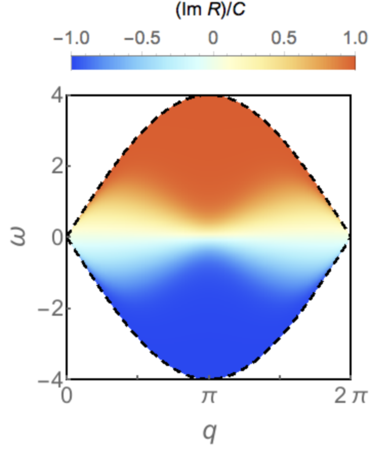
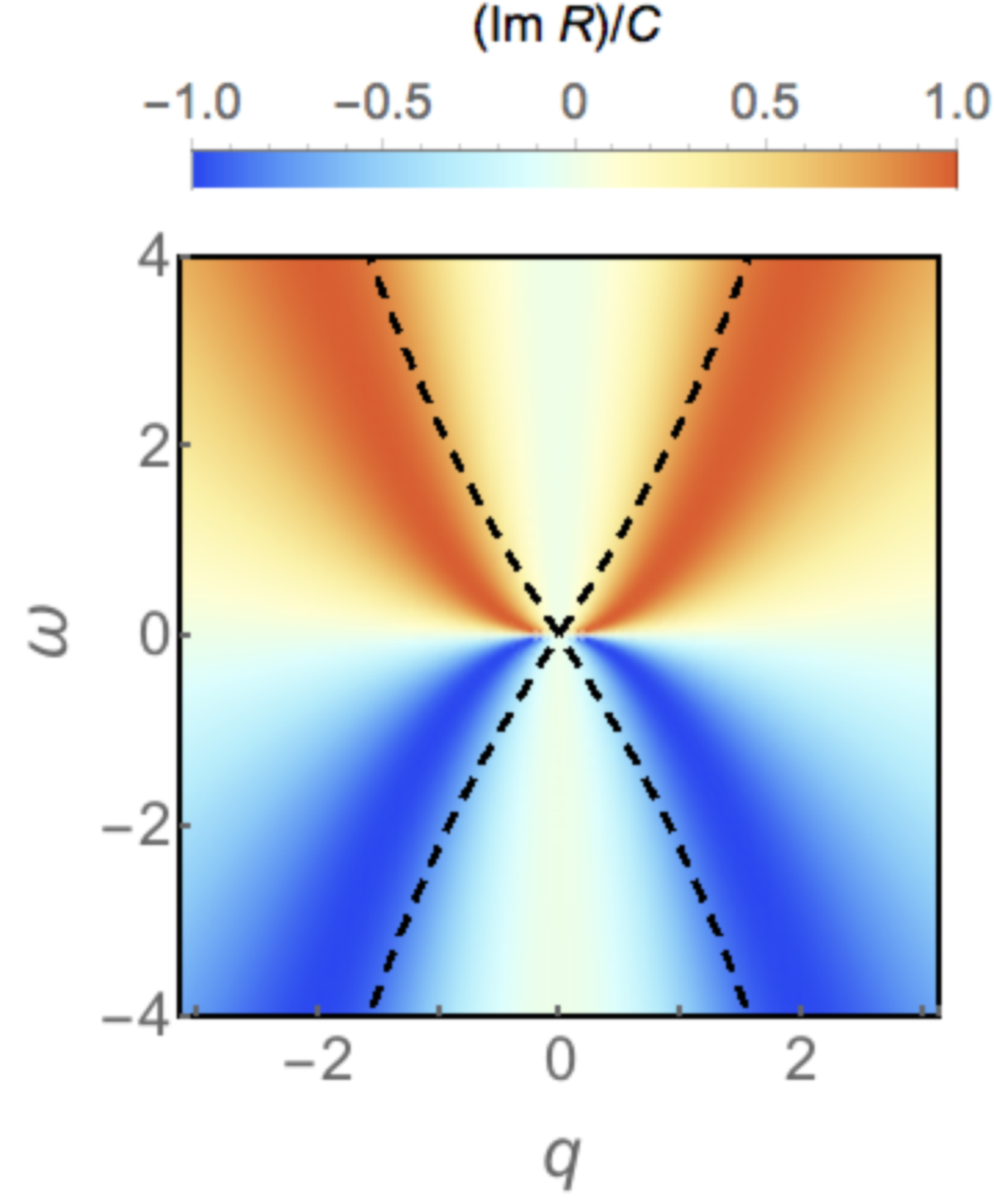
Figure 1: (Color online) Contour plots of $\text{Im}\,R(q,\omega)/C(q,\omega)$ as a function of $q$ and $\omega$ for the quench of hard-core bosons in the superlattice potential with $\Delta=0.5$ (left) and for the Lieb-Liniger model (right). The dashed lines indicate the values of this ratio which are relevant for determining $\lambda_{k}$’s, as explained in the main text. Due to the presence of the lattice, the ratio on the left panel is defined only within the domain shown.

IV Conclusions

We have explained how the complete set of Lagrange multipliers $\lambda_{k}$’s of a GGE can be obtained at once from a single measurement of time-delayed correlation and linear response functions of suitable physical observables, that are within experimental reach. We focused our analysis on the steady state of integrable systems but our arguments are sufficiently general to be also applicable to quasi-stationary prethermal states described by a GGE. Although we discussed primarily quenches from ground states, the proposed approach is viable also for generic initial states, including thermal ones. In practice, having in mind the experimental setting of Ref. GGE-exp , one should measure the space-time dependent correlation and response functions of the bosonic density and calculate their Fourier transforms in both space and time. By sweeping the corresponding momenta and frequencies in the manner described above for, e.g., the Lieb-Liniger model, one then extracts all $\lambda_{k}$’s.

We are currently working on the extension of these ideas to interacting systems, such as quenches to generic $c$ in the integrable Lieb-Liniger model in Eq. (23) — using methods employed in Ref. vandenBerg ; Jacopo or the quench action approach QAreview — or in the solvable $O(N)$ model for $N\to\infty$, which features a variety of dynamical phases with different properties but has no obvious GGE description, see, e.g., Refs. Chandran ; Chiocchetta .

Appendix A Quench of the Ising spin chain

This Appendix provides some details on the solution of the analysis of the quantum Ising spin chain. We recall in Sec. A.1 the solution of the post-quench dynamics of this model. In Sec. A.2 we calculate the correlation and response functions of the transverse magnetization, and we show how the Lagrange multipliers $\lambda_{k}$ of the GGE of can be determined on the basis of their FDR.

A.1 Post-quench dynamics

The Hamiltonian of the quantum Ising spin chain, reported in Eq. (27), can be diagonalized by means of a Jordan-Wigner transformation and a Fourier transform which maps spins into fermions $\{\hat{c}_{k},\hat{c}_{-k}^{\dagger}\}_{k}$. The dynamics of these fermions after a quench of the transverse field $\Gamma_{0}\to\Gamma$ can be exactly determined in terms of the quasi-particles $\{\hat{\gamma}_{k}^{\Gamma_{0}},\hat{\gamma}_{-k}^{\Gamma_{0}\,{\dagger}}\}_{k}$ which diagonalize the pre-quench Hamiltonian $\hat{H}(\Gamma_{0})$, as explained, e.g., in Ref. Foini12 , which we refer to for additional details as well as for the notation adopted here. In particular, the evolution of the fermions reads:

$$\left(\begin{array}[]{c}\hat{c}_{k}(t)\\[5.69054pt] \hat{c}_{-k}^{{\dagger}}(t)\end{array}\right)=\left(\begin{array}[]{cc}u_{k}^{\Gamma,\Gamma_{0}}(t)&-[v_{k}^{\Gamma,\Gamma_{0}}(t)]^{*}\\[5.69054pt] v_{k}^{\Gamma,\Gamma_{0}}(t)&[u_{k}^{\Gamma,\Gamma_{0}}(t)]^{*}\end{array}\right)\left(\begin{array}[]{c}\hat{\gamma}_{k}^{\Gamma_{0}}\\[5.69054pt] \hat{\gamma}_{-k}^{\Gamma_{0}\;{\dagger}}\end{array}\right),$$ (31)

where

$$\begin{cases}\displaystyle u_{k}^{\Gamma,\Gamma_{0}}(t)=e^{-i\epsilon^{\Gamma}_{k}t}\cos\theta_{k}^{\Gamma}\cos(\theta_{k}^{\Gamma}-\theta_{k}^{\Gamma_{0}})+e^{i\epsilon^{\Gamma}_{k}t}\sin\theta_{k}^{\Gamma}\sin(\theta_{k}^{\Gamma}-\theta_{k}^{\Gamma_{0}}),\\ \displaystyle v_{k}^{\Gamma,\Gamma_{0}}(t)=ie^{-i\epsilon^{\Gamma}_{k}t}\sin\theta_{k}^{\Gamma}\cos(\theta_{k}^{\Gamma}-\theta_{k}^{\Gamma_{0}})-ie^{i\epsilon^{\Gamma}_{k}t}\cos\theta_{k}^{\Gamma}\sin(\theta_{k}^{\Gamma}-\theta_{k}^{\Gamma_{0}}),\end{cases}$$ (32)

with $\epsilon^{\Gamma}_{k}\equiv\epsilon_{k}(\Gamma)=2\sqrt{1+\Gamma^{2}-2\Gamma\cos k}$, while the so-called Bogoliubov angles $\theta_{k}^{\Gamma,\Gamma_{0}}$ are determined by solving $\tan(2\theta_{k}^{\Gamma})=(\sin k)/(\Gamma-\cos k)$, with the important property that $\theta_{-k}^{\Gamma}=-\theta_{k}^{\Gamma}$, which turns out to be useful later on. The initial state of the evolution, i.e., the ground state of the pre-quench Hamiltonian $\hat{H}(\Gamma_{0})$ is actually the vacuum of the fermionic quasi-particles $\{\hat{\gamma}_{k}^{\Gamma_{0}},\hat{\gamma}_{-k}^{\Gamma_{0}\,{\dagger}}\}_{k}$. For convenience, below we denote by $\Delta_{k}\equiv\theta_{k}^{\Gamma}-\theta_{k}^{\Gamma_{0}}$ the difference between the angles appearing in Eq. (32), which however differs from the notation $\Delta_{k}\equiv 2(\theta_{k}^{\Gamma}-\theta_{k}^{\Gamma_{0}})$ used in Ref. Foini12 .

A.2 FDR for the transverse magnetization

According to the definition of $\hat{M}^{z}_{q}$ in Eq. (29), we consider the quantity,

$$\begin{split}&\langle\hat{M}^{z}_{q}(t_{1})\hat{M}^{z}_{-q}(t_{2})\rangle_{c}=\\ &=\langle\hat{M}^{z}_{q}(t_{1})\hat{M}^{z}_{-q}(t_{2})\rangle-\langle\hat{M}^{z}_{q}(t_{1})\rangle\langle\hat{M}^{z}_{-q}(t_{2})\rangle\\ &=4\sum_{k_{1},k_{2}}\ \langle\hat{c}^{{\dagger}}_{k_{1}+q}(t_{1})\hat{c}_{k_{1}}(t_{1})\hat{c}^{{\dagger}}_{k_{2}}(t_{2})\hat{c}_{k_{2}+q}(t_{2})\rangle,\end{split}$$ (33)

where we used the fact that $\hat{\sigma}^{z}_{j}=1-2\hat{c}^{\dagger}_{j}\hat{c}_{j}$ in terms of the fermions, see, e.g., Ref. Foini12 . Substituting the explicit expressions for the evolution of the fermionic operators provided by Eq. (31) and taking the expectation value on the pre-quench ground state, one obtains (for $q\neq 0$, with additional contributions for $q=0$)

$$\langle\hat{M}^{z}_{q}(t_{1})\hat{M}^{z}_{-q}(t_{2})\rangle_{c}=4(A+B),$$ (34)

with

$$A\equiv\sum_{k}\ v_{k+q}(t_{1})u_{k}(t_{1})u_{k}^{\ast}(t_{2})v_{k+q}^{\ast}(t_{2})$$ (35)

and

$$B\equiv\sum_{k}\ v_{k+q}(t_{1})u_{k}(t_{1})u_{k+q}^{\ast}(t_{2})v_{k}^{\ast}(t_{2}).$$ (36)

In order to simplify the notation, we omitted the superscripts $\Gamma,\Gamma_{0}$ from Eq. (31). We are interested in the stationary limit of the correlation function in Eq. (34). Keeping solely the terms that depend only on $t\equiv t_{2}-t_{1}$, one obtains

$$\begin{split}\displaystyle A=\sum_{k}&\Big{[}e^{i(\epsilon_{k+q}+\epsilon_{k})t}\left(\sin\theta_{k+q}\cos\Delta_{k+q}\cos\theta_{k}\cos\Delta_{k}\right)^{2}+e^{i(\epsilon_{k+q}-\epsilon_{k})t}\left(\sin\theta_{k+q}\cos\Delta_{k+q}\sin\theta_{k}\sin\Delta_{k}\right)^{2}\\ &+e^{-i(\epsilon_{k+q}-\epsilon_{k})t}\left(\cos\theta_{k+q}\sin\Delta_{k+q}\cos\theta_{k}\cos\Delta_{k}\right)^{2}+e^{-i(\epsilon_{k+q}+\epsilon_{k})t}\left(\cos\theta_{k+q}\sin\Delta_{k+q}\sin\theta_{k}\sin\Delta_{k}\right)^{2}\Big{]}\end{split}$$ (37)

$$\begin{split}\displaystyle B=&\displaystyle\sum_{k}\Big{[}e^{i(\epsilon_{k+q}+\epsilon_{k})t}\sin\theta_{k}\cos^{2}\Delta_{k}\cos\theta_{k+q}\sin\theta_{k+q}\cos^{2}\Delta_{k+q}\cos\theta_{k}\\ &\displaystyle\qquad-e^{-i(\epsilon_{k+q}-\epsilon_{k})t}\sin\theta_{k}\cos^{2}\Delta_{k}\cos\theta_{k+q}\sin\theta_{k+q}\sin^{2}\Delta_{k+q}\cos\theta_{k}\\ &\displaystyle\qquad-e^{i(\epsilon_{k+q}-\epsilon_{k})t}\cos\theta_{k}\sin^{2}\Delta_{k}\cos\theta_{k+q}\sin\theta_{k+q}\cos^{2}\Delta_{k+q}\sin\theta_{k}\\ &\displaystyle\qquad+e^{-i(\epsilon_{k+q}+\epsilon_{k})t}\cos\theta_{k}\sin^{2}\Delta_{k}\cos\theta_{k+q}\sin\theta_{k+q}\sin^{2}\Delta_{k+q}\sin\theta_{k}\Big{]},\end{split}$$ (38)

where, for convenience, we simplified the notation by omitting the superscript $\Gamma$ in $\epsilon^{\Gamma}_{k}$, as no confusion can arise. Accordingly, the stationary part of Eq. (34) is given by $\langle\hat{M}^{z}_{q}(t_{1})\hat{M}^{z}_{-q}(t_{2})\rangle_{c}^{\text{stat}}=4\sum_{k}\left[A_{12}^{(1)}+B_{12}^{(1)}+B_{12}^{(2)}+A_{12}^{(2)}\right]$ where

$$\begin{split}&A_{12}^{(1)}=e^{i(\epsilon_{k+q}+\epsilon_{k})t}\cos^{2}\Delta_{k}\sin\theta_{k+q}\cos^{2}\Delta_{k+q}\cos\theta_{k}\sin(\theta_{k}+\theta_{k+q})\\ &B_{12}^{(1)}=e^{-i(\epsilon_{k+q}-\epsilon_{k})t}\cos^{2}\Delta_{k}\cos\theta_{k+q}\sin^{2}\Delta_{k+q}\cos\theta_{k}\cos(\theta_{k}+\theta_{k+q})\\ &B_{12}^{(2)}=\displaystyle e^{i(\epsilon_{k+q}-\epsilon_{k})t}\sin^{2}\Delta_{k}\sin\theta_{k+q}\cos^{2}\Delta_{k+q}\sin\theta_{k}(-\cos(\theta_{k+q}+\theta_{k}))\\ &A_{12}^{(2)}=\displaystyle e^{-i(\epsilon_{k+q}+\epsilon_{k})t}\sin^{2}\Delta_{k}\cos\theta_{k+q}\sin^{2}\Delta_{k+q}\sin\theta_{k}\sin(\theta_{k+q}+\theta_{k}).\end{split}$$ (39)

The correlation and response functions $C$ and $R$ of the magnetization $\hat{M}^{z}_{q}$ are defined, as usual, using the commutator and anti-commutator of $\hat{M}^{z}_{q}(t_{1})$ and $\hat{M}^{z}_{-q}(t_{2})$ [see Eqs. (2) and (3)], which can be determined from the previous expressions. In particular, considering the commutator and anti-commutator $\langle\hat{M}^{z}_{q}(t_{1})\hat{M}^{z}_{-q}(t_{2})\rangle_{c}^{\text{stat}}\mp\langle\hat{M}^{z}_{-q}(t_{2})\hat{M}^{z}_{q}(t_{1})\rangle_{c}^{\text{stat}}$ one has, respectively:

$$\begin{split}A_{12}^{(1)}\mp A_{21}^{(1)}+A_{12}^{(2)}\mp A_{21}^{(2)}&=\sin(\theta_{k}+\theta_{k+q})\left(\cos^{2}\Delta_{k}\cos^{2}\Delta_{k+q}\mp\sin^{2}\Delta_{k}\sin^{2}\Delta_{k+q}\right)\\ &\qquad\times\left[e^{i(\epsilon_{k}+\epsilon_{k+q})t}\sin\theta_{k+q}\cos\theta_{k}\mp e^{-i(\epsilon_{k}+\epsilon_{k+q})t}\cos\theta_{k+q}\sin\theta_{k}\right]\end{split}$$ (40)

$$\begin{split}B_{12}^{(1)}\mp B_{21}^{(1)}+B_{12}^{(2)}\mp B_{21}^{(2)}&=\cos(\theta_{k}+\theta_{k+q})\left(\cos^{2}\Delta_{k}\sin^{2}\Delta_{k+q}\mp\sin^{2}\Delta_{k}\cos^{2}\Delta_{k+q}\right)\\ &\qquad\qquad\times\left[e^{i(\epsilon_{k}-\epsilon_{k+q})t}\cos\theta_{k+q}\cos\theta_{k}-e^{-i(\epsilon_{k}-\epsilon_{k+q})t}\sin\theta_{k+q}\sin\theta_{k}\right],\end{split}$$ (41)

where $A^{(i)}_{21}$ and $B^{(i)}_{21}$ are obtained from the corresponding $A^{(i)}_{12}$ and $B^{(i)}_{12}$ by replacing $t$ with $-t$ and by exchanging the subscripts $k+q$ and $k$ in the previous expressions. Taking the Fourier transform in time of the stationary parts of $C(t_{2},t_{1})$ and $R(t_{2},t_{1})$ one obtains the corresponding two expressions $C(q,\omega)$ and $R(q,\omega)$ which depend also on the specific value of $q$ and involve a sum over $k$ of a linear combination of $\delta(\omega\pm(\epsilon_{k}+\epsilon_{k+q}))$ and $\delta(\omega\pm(\epsilon_{k}-\epsilon_{k+q}))$ resulting from the Fourier transform of the exponentials in the previous expressions. We first note that if $\omega>0$ and $q$ are chosen in such a way that $\text{Im}\,R(q,\omega)$ and $C(q,\omega)$ receive contributions from $\delta(\omega-(\epsilon_{k}+\epsilon_{k+q}))$, then the remaining $\delta$’s do not contribute, as $\epsilon_{k}+\epsilon_{k+q}>|\epsilon_{k}-\epsilon_{k+q}|$ for $k\neq 0$. On the other hand, for a given $\omega$ and $q$, if a certain value $k^{\prime}$ of the index $k$ of the sum contributes to $C$ and $R$ because $\omega=\epsilon_{k^{\prime}}+\epsilon_{k^{\prime}+q}$, then also $-k^{\prime}-q+2\pi n$ (with integer $n$) does. This means that, generically, the condition:

$$\omega=\omega_{k,q}\equiv\epsilon_{k}+\epsilon_{k+q}$$ (42)

is satisfied (depending on $q$ and $\omega$) by either none or an even number of values of $k\in[0,2\pi]$, with at most four values, as a direct inspection of Eq. (42) as well as Fig. 2 show.

​​ ​​

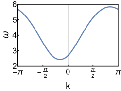
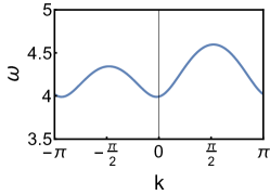
Figure 2: (Color online) Plot of the dependence of $\omega=\epsilon_{k}+\epsilon_{k+q}$ on $k$ for $q=1$ (left) and $q=3$ (right), with $\Gamma=1/2$. For sufficiently large values of $q$, i.e., $|q|>q_{\rm max}$ (see the main text) there is a wide range of values of $\omega$ for which more than two values of $k$ satisfy Eq. (42).

In particular, from a more careful analysis of Eq. (42), one concludes that for $|q|<q_{\rm max}$ with $q_{\rm max}=2\arccos\rm{min}\{\Gamma,\Gamma^{-1}\}$, the equation has at most two solutions which are related as discussed above. Based on this relationship and on the symmetry properties of the Bogoliubov angles, one immediately concludes that these two selected values of $k$ results in the same contribution both to $C$ and to $\text{Im}\,R$ and therefore

$$\begin{split}\frac{\text{Im}\,R(q,\omega_{k,q})}{C(q,\omega_{k,q})}&=\frac{\sin(\theta_{k}+\theta_{{k}+q})\left(\sin\theta_{{k}+q}\cos\theta_{k}+\sin\theta_{k}\cos\theta_{k+q}\right)\left(\cos^{2}\Delta_{{k}+q}\cos^{2}\Delta_{k}-\sin^{2}\Delta_{{k}+q}\sin^{2}\Delta_{k}\right)}{\sin(\theta_{k}+\theta_{{k}+q})\left(\sin\theta_{k+q}\cos\theta_{k}+\sin\theta_{k}\cos\theta_{k+q}\right)\left(\cos^{2}\Delta_{{k}+q}\cos^{2}\Delta_{k}+\sin^{2}\Delta_{{k}+q}\sin^{2}\Delta_{k}\right)}\\ &=\frac{\cos^{2}\Delta_{{k}+q}\cos^{2}\Delta_{k}-\sin^{2}\Delta_{{k}+q}\sin^{2}\Delta_{k}}{\cos^{2}\Delta_{{k}+q}\cos^{2}\Delta_{k}+\sin^{2}\Delta_{{k}+q}\sin^{2}\Delta_{k}}\\ &=\displaystyle\frac{\cos(2\Delta_{k+q})+\cos(2\Delta_{k})}{1+\cos(2\Delta_{k+q})\cos(2\Delta_{k})}=\tanh\left(\frac{\lambda_{k}+\lambda_{k+q}}{2}\right),\end{split}$$ (43)

where in the last step we have used the fact that $\cos(2\Delta_{k})=\tanh(\lambda_{k}/2)$ Foini12 . In particular, taking into account that $\lambda_{k}=\lambda_{-k}$, one can use the previous relationship in order to extract some of the $\lambda_{k}$’s, e.g., by choosing $q=-2k$, with $\omega=\omega_{k,-2k}=2\epsilon_{k}$ and $|k|<q_{\rm max}/2$. For $|q|>q_{\rm max}$, instead, Eq. (42) can have more than two solutions (see Fig. 2) which are not all related as discussed above and therefore the corresponding contributions to the correlation and response functions are not necessarily equal and the resulting ratio $\text{Im}\,R/C$ depends in general also on $\theta_{k}$.

References

• (1) A. Polkovnikov, K. Sengupta, A. Silva, and M. Vengalattore, Nonequilibrium dynamics of isolated interacting quantum systems, Rev. Mod. Phys. 83, 863 (2011).
• (2) Quantum integrability in out-of-equilibrium systems, J. Stat. Mech. 064001 – 064011 (2016), Special Issue, P. Calabrese, F. H. L. Essler and G. Mussardo eds.
• (3) C. Gogolin and J. Eisert, Equilibration, thermalisation, and the emergence of statistical mechanics in closed quantum systems, Rep. Prog. Phys. 79, 056001 (2016).
• (4) M. Rigol, V. Dunjko, V. Yurovsky, and M. Olshanii, Relaxation in a completely integrable many-body quantum system: An ab initio study of the dynamics of the highly excited states of 1D lattice hard-core bosons, Phys. Rev. Lett. 98, 050405 (2007).
M. Rigol, V. Dunjko, and M. Olshanii, Thermalization and its mechanism for generic isolated quantum systems, Nature 452, 854 (2008).
• (5) E. Ilievski, M. Medenjak, T. Prosen, and L. Zadnik, Quasilocal charges in integrable lattice systems, J. Stat. Mech. 064008 (2016) and refs. therein.
• (6) E. Ilievski, J. De Nardis, B. Wouters, J.-S. Caux, F. H. L. Essler, T. Prosen, Complete Generalized Gibbs Ensembles in an Interacting Theory, Phys. Rev. Lett. 115, 157201 (2015).
• (7) J.-S. Caux, R. M. Konik, Constructing the generalized Gibbs ensemble after a quantum quench, Phys. Rev. Lett. 109, 175301 (2012).
• (8) T. Langen, S. Erne, R. Geiger, B. Rauer, T. Schweigler, M. Kuhnert, W. Rohringer, I. E. Mazets, T. Gasenzer, J. Schmiedmayer, Experimental observation of a generalized Gibbs ensemble, Science 348, 207-211 (2015).
• (9) R. Kubo, The fluctuation-dissipation theorem, Rep. Prog. Phys. 29, 255-284 (1966).
• (10) L. F. Cugliandolo, The effective temperature, J. Phys. A 44, 483001 (2011).
• (11) J. M. Deutsch, Quantum statistical mechanics in a closed system, Phys. Rev. A 43, 2046 (1991).
• (12) M. Srednicki, Chaos and quantum thermalization, Phys. Rev. E 50, 888 (1994).
• (13) E. Khatami, G. Pupillo, M. Srednicki, and M. Rigol, Fluctuation-Dissipation Theorem in an Isolated System of Quantum Dipolar Bosons after a Quench, Phys. Rev. Lett. 111, 050403 (2013).
• (14) L. F. Cugliandolo, J. Kurchan, and L. Peliti, Energy flow, partial equilibration, and effective temperatures in systems with slow dynamics, Phys. Rev. E 55, 3898 (1997).
L. F. Cugliandolo and J. Kurchan, A scenario for the dynamics in the small entropy production limit, J. Phys. Soc. Japan 69, 247 (2000).
• (15) P. Calabrese and A. Gambassi, Ageing properties of critical systems, J. Phys. A 38, R133 (2005); On the definition of a unique effective temperature for non-equilibrium critical systems, J. Stat. Mech. P07013 (2004).
• (16) P. Calabrese and J. Cardy, Quantum quenches in extended systems, J. Stat. Mech. P06008 (2007).
• (17) S. Sotiriadis, P. Calabrese and J. Cardy, Quantum quench from a thermal initial state, EPL 87, 20002 (2009).
• (18) A. Mitra and T. Giamarchi, Mode-coupling-induced dissipative and thermal effects at long times after a quantum quench, Phys. Rev. Lett. 107, 150602 (2011).
• (19) M. Rigol, A. Muramatsu, and M. Olshanii, Hard-core bosons on optical superlattices: Dynamics and relaxation in the superfluid and insulating regimes, Phys. Rev. A 74, 053616 (2006).
• (20) M.-C. Chung, A. Iucci and M. A. Cazalilla, Thermalization in systems with bipartite eigenmode entanglement, New J. Phys. 14, 075013 (2012).
• (21) T. S. Bortolin and A. Iucci, Effective temperature from fluctuation-dissipation theorem in systems with bipartite eigenmode entanglement, Phys. Rev. B 91, 024301 (2015).
• (22) E. H. Lieb and W. Liniger, Exact analysis of an interacting Bose gas. I. The general solution and the ground state, Phys. Rev. 130, 1605 (1963); E. H. Lieb, Exact analysis of an interacting Bose gas. II. The excitation spectrum, Phys. Rev. 130, 1616 (1963).
• (23) M. Kormos, M. Collura, P. Calabrese, Analytic results for a quantum quench from free to hard-core one-dimensional bosons, Phys. Rev. A 89, 013609 (2014).
• (24) Pasquale Calabrese, Fabian H.L. Essler, and Maurizio Fagotti, Quantum Quench in the Transverse Field Ising Chain II: Stationary State Properties, J. Stat. Mech. P07022 (2012).
• (25) D. Karevski, Ising quantum chains, arXiv: cond-mat/ 0611327 (2006).
• (26) J. Dziarmaga, Dynamics of a quantum phase transition and relaxation to a steady state, Adv. Phys. 59, 1063 (2010).
• (27) A. Dutta, G. Aeppli, B. K. Chakrabarti, U. Divakaran, T. F. Rosenbaum and D. Sen, Quantum phase transitions in transverse field spin models: From Statistical Physics to Quantum Information, (Cambridge Univ. Press, Cambridge, 2015).
• (28) L. Foini, L. F. Cugliandolo, and A. Gambassi, Fluctuation-dissipation relations and critical quenches in the transverse field Ising chain, Phys. Rev. B 84, 212404 (2011).
• (29) L. Foini, L. F. Cugliandolo, and A. Gambassi, Dynamic correlations, fluctuation-dissipation relations, and effective temperatures after a quantum quench of the transverse field Ising chain, J. Stat. Mech. P09011 (2012).
• (30) R. van den Berg, B. Wouters, S. Eliëns, J. De Nardis, R. M. Konik, J.-S. Caux, Separation of Timescales in a Quantum Newton’s Cradle, Phys. Rev. Lett. 116, 225302 (2016)
• (31) J. De Nardis, B. Wouters, M. Brockmann, J.-S. Caux, Solution for an interaction quench in the Lieb-Liniger Bose gas. Phys. Rev. A 89, 033601 (2014).
• (32) J.-S. Caux, The Quench Action, J. Stat. Mech. 064006 (2016).
• (33) A. Chandran, A. Nanduri, S. S. Gubser, and S. L. Sondhi, Equilibration and coarsening in the quantum $O(N)$ model at infinite $N$, Phys. Rev. B 88, 024306 (2013).
• (34) A. Maraga, A. Chiocchetta, A. Mitra, and A. Gambassi, Aging and coarsening in isolated quantum systems after a quench: exact results for the quantum $O(N)$ model with $N\to\infty$, Phys. Rev. E 92, 042151 (2015).