Finite Element Formulation for a Poroelasticity Problem Stemming from Mixture Theory

Abstract

A finite element formulation is developed for a poroelastic medium consisting of an incompressible hyperelastic skeleton saturated by an incompressible fluid. The governing equations stem from mixture theory and the application is motivated by the study of interstitial fluid flow in brain tissue. The formulation is based on the adoption of an arbitrary Lagrangian-Eulerian (ALE) perspective. We focus on a flow regime in which inertia forces are negligible. The stability and convergence of the formulation is discussed, and numerical results demonstrate agreement with the theory.

Keywords: Finite Element Method; Theory of Mixtures; Poroelasticity

1 Introduction

A central problem in brain physiology is the transport of metabolites produced by cell functions in brain tissue from their production site to the main cerebrospinal fluid (CSF) compartment (Iliff et al., 2012; Iliff et al., 2013, 2013; Iliff and Nedergaard, 2013). The modeling of these transport phenomena has traditionally focused on Fickian diffusion within the extracellular space (Syková, 2004; Syková and Nicholson, 2008; Vargova and Syková, 2011; Vargova et al., 2011) (see also Gevertz and Torquato, 2008). More recently, the studies by Iliff and co-workers (Iliff et al., 2012; Iliff et al., 2013, 2013; Iliff and Nedergaard, 2013) point to the existence of pathways for metabolite exchange with significant convective transport. Furthermore, evidence indicates that such convective component is driven by the pulsatile motion of arterial walls along the various elements of the brain vascular tree.

The coupling between transport and mechanical properties is a fundamental aspect of the design of tissue engineered scaffolds, especially for application in the regeneration of peripheral nerves (Saracino et al., 2013; Dey et al., 2008; Dey et al., 2010; Nguyen et al., 2015). In these applications, it is essential to coordinate the evolution of the transport and mechanical properties with the rate of degradation of the material. Modeling of these systems requires a framework for the system’s poroelastic behavior along with the reaction-diffusion physics of the degradation process.

Motivated by these these problems, we considered transport models that could simultaneously include both diffusive and convective components. The models must also have the ability to characterize the flow field of specific molecular constituents and their interaction with large deformations. Finally, we needed models that can be expanded to include chemical reactions.. For these reasons, we focused on a model of transport in poroelastic media based on mixture theory (Bowen, 1976, 1980, 1982; Rajagopal and Tao, 1995).

There is a significant body of literature on numerical methods for flow in porous media and poroelasticity (see, e.g., Selvadurai, 1996; Lewis and Shrefler, 1998; Armero, 1999; Coussy, 2010), but we found limited work when such phenomena are studied from a mixture theory perspective, i.e., by considering the simultaneous existence of multiple independent velocity fields, as they appear in mixture theory. In this paper we present our experience in formulating a mixed finite element method (FEM) for a simple mixture consisting of an incompressible hyperelastic solid skeleton saturated by an incompressible fluid. Our focus is to determine the fluid flow in addition to the filtration velocity. In future developments, we plan to combine the porous flow problem with a convection-reaction-diffusion component for the species present in the fluid. Hence, our quantities of interest are the pore pressure, the velocity fields of the fluid and solid phases, the filtration velocity, as well as the displacement field of the solid phase. The incompressibility of the constituents yields a constraint equation, which, when expressed in the body’s current configuration, requires the volume-fraction-average of the solid and fluid velocity fields to be divergence-free. Perhaps the most delicate aspect of the enforcement of this condition is the fact that the action of the divergence operator affects the porosity field in addition to the velocities. From an experimental viewpoint, this field might have significant uncertainty in its determination. To avoid dealing with gradients of the porosity we have considered two strategies: (i) selecting four fields as primary unknowns, namely the solid displacement, solid velocity, fluid velocity, and pore pressure, along with weakening the constraint equation using the divergence theorem; and (ii) modifying this formulation by replacing the fluid velocity with the filtration velocity as a primary field. In the first approach the filtration velocity can be determined during post-processing as a simple $L^{2}$-projection. Fluid velocity is recovered in an analogous manner in the second approach. We will discuss the advantages and disadvantages of both strategies. As it turns out, the second strategy offers a coercivity property that is stronger than the first and can possibly justify such an approach in practice. The first strategy does not appear to work well unless properly stabilized. We have implemented stabilization in both strategies for the quasi-static motion of a nonlinear poroelastic body. In particular, we have adapted to the present context the stabilization strategy demonstrated by Masud and Hughes (2002) (see also Masud, 2007).

We point out that there are various flow regimes of interest. Specifically, there are conditions in which it is reasonable to assume that inertia effects are negligible and that therefore the evolution of the system is quasi-static. On the other hand, there are some flow regimes in which it is desirable to account for inertia effects. With this in mind, the work in the paper is limited to the analysis of the quasi-static approximation of the problem. The fully dynamic case will be considered in future publications.

2 Basic definitions and governing equations

2.1 Configurations, motions, volume fractions, and incompressibility

With reference to Fig. 1,

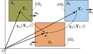
Figure 1: Current configuration $B_{t}$ of a binary mixture consisting of a solid skeleton and a fluid. $B_{t}$ is the common image of the two motions $\boldsymbol{\chi}_{\mathrm{s}}$ and $\boldsymbol{\chi}_{\mathrm{f}}$ of the solid skeleton and the fluid, respectively.

we consider the deformed configuration of a porous body $B_{t}$ saturated by an incompressible fluid. The solid phase is assumed to be hyperelastic and incompressible. To describe the motion of the system, we adopt the theoretical setting in Bowen (1980) (see also Bowen, 1976). Hence, $B_{t}$ is the common image of two diffeomorphisms: $\boldsymbol{\chi}_{\mathrm{s}}:B_{\mathrm{s}}\times[0,T]\to B_{t}\subset\mathscr{E}^{d}$ and $\boldsymbol{\chi}_{\mathrm{f}}:B_{\mathrm{f}}\times[0,T]\to B_{t}\subset\mathscr{E}^{d}$, where $B_{\mathrm{s}}$ and $B_{\mathrm{f}}$ are the reference configurations of the solid and fluid phases, respectively, $t\in[0,T]$, with $[0,T]$ a chosen time interval of interest. By $\mathscr{E}^{d}$, with $n=2,3$, we denote the $d$-dimensional Euclidean point space and by $\mathscr{T}^{d}$ its companion translation vector space. The subscripts ‘$\mathrm{s}$’ and ‘$\mathrm{f}$’ stand for ‘solid’ and ‘fluid’, respectively. Points in $B_{\mathrm{s}}$ and $B_{\mathrm{f}}$ will be denoted by $\boldsymbol{X}_{\mathrm{s}}$ and $\boldsymbol{X}_{\mathrm{f}}$, respectively, whereas $\boldsymbol{x}$ denotes position in $B_{t}$. $\partial B_{\mathrm{s}}$, $\partial B_{\mathrm{f}}$, $\partial B_{t}$ are the boundaries of $B_{\mathrm{s}}$, $B_{\mathrm{f}}$ and $B_{t}$, respectively, oriented by corresponding outward unit normal fields $\boldsymbol{n}_{\mathrm{s}}$, $\boldsymbol{n}_{\mathrm{f}}$, and $\boldsymbol{n}$.

For simplicity, the initial configurations for the solid and fluid are made to coincide with the initial configuration of the mixture, so that

$$B_{\mathrm{s}}=B_{\mathrm{f}}=B_{t}\big{|}_{t=0}.$$ (1)

For each constituent $a=\mathrm{s},\mathrm{f}$, the displacement, deformation gradient, and Jacobian determinant of the motions are, respectively,

$$\boldsymbol{u}_{a}(\boldsymbol{X}_{a},t)\coloneqq\boldsymbol{\chi}_{a}(\boldsymbol{X}_{a},t)-\boldsymbol{X}_{a},\quad\mathsf{F}_{a}(\boldsymbol{X}_{a},t)\coloneqq\frac{\partial\boldsymbol{\chi}_{a}(\boldsymbol{X}_{a},t)}{\partial\boldsymbol{X}_{a}},\quad J_{a}(\boldsymbol{X}_{a},t)\coloneqq\det{\mathsf{F}_{a}(\boldsymbol{X}_{a},t)},$$ (2)

where, $\forall\boldsymbol{X}_{a}\in B_{a}$ and $\forall t\in[0,t]$, $J_{a}(\boldsymbol{X}_{a},t)>0$.

The spatial (or Eulerian) representation of the material velocity of constituent $a$ ($a=\mathrm{s},\mathrm{f}$) is

$$\boldsymbol{v}_{a}(\boldsymbol{x},t)\coloneqq\frac{\partial\boldsymbol{\chi}_{a}(\boldsymbol{X}_{a},t)}{\partial t}\bigg{|}_{\boldsymbol{X}_{a}=\boldsymbol{\chi}_{a}^{-1}(\boldsymbol{x},t)}=\frac{\partial\boldsymbol{u}_{a}(\boldsymbol{X}_{a},t)}{\partial t}\bigg{|}_{\boldsymbol{X}_{a}=\boldsymbol{\chi}_{a}^{-1}(\boldsymbol{x},t)},\quad\forall\boldsymbol{x}\in B_{t}.$$ (3)

We note that, in principle, it is possible to express the displacement field in Eulerian form, that is by writing

$$\boldsymbol{u}_{a}(\boldsymbol{x},t)\coloneqq\boldsymbol{x}-\boldsymbol{\chi}_{a}^{-1}(\boldsymbol{x},t),$$ (4)

where, with a slight abuse of notation, we are using the symbol $\boldsymbol{u}_{a}$ to refer to the displacement field whether described in Lagrangian or Eulerian form and relying on the context to resolve the ambiguity. With this in mind, for future reference we note that

$$\mathsf{F}_{\mathrm{s}}(\boldsymbol{X},t)\big{|}_{\boldsymbol{X}=\boldsymbol{\chi}_{\mathrm{s}}^{-1}(\boldsymbol{x},t)}=(\mathsf{I}-\operatorname{\nabla_{\!\boldsymbol{x}}}\boldsymbol{u}_{\mathrm{s}})^{-1},$$ (5)

where $\operatorname{\nabla_{\!\boldsymbol{x}}}$ is the gradient with respect to $\boldsymbol{x}$ over $B_{t}$. Denoting the material time derivative following the motion of phase $a$ by $D_{t_{a}}$, recalling that $\boldsymbol{v}_{\mathrm{s}}$ is the material time derivative of $\boldsymbol{u}_{\mathrm{s}}$, in an Eulerian context, for all $\boldsymbol{x}\in B_{t}$, we must have

$$D_{t_{\mathrm{s}}}\boldsymbol{u}_{\mathrm{s}}=\boldsymbol{v}_{\mathrm{s}}\quad\Rightarrow\quad\partial_{t}\boldsymbol{u}_{\mathrm{s}}+(\operatorname{\nabla_{\!\boldsymbol{x}}}\boldsymbol{u}_{\mathrm{s}})\boldsymbol{v}_{\mathrm{s}}=\boldsymbol{v}_{\mathrm{s}}\quad\Rightarrow\quad\boldsymbol{v}_{\mathrm{s}}=(\mathsf{I}-\operatorname{\nabla_{\!\boldsymbol{x}}}\boldsymbol{u}_{\mathrm{s}})^{-1}\partial_{t}\boldsymbol{u}_{\mathrm{s}},$$ (6)

which, again, requires the invertibility of $\mathsf{I}-\operatorname{\nabla_{\!\boldsymbol{x}}}\boldsymbol{u}_{\mathrm{s}}$. For future reference, we note that the Lagrangian expression of the above relation is: for all $\boldsymbol{X}_{\mathrm{s}}\in B_{\mathrm{s}}$ and $t\in(0,T)$, we must have

$$D_{t_{\mathrm{s}}}\boldsymbol{u}_{\mathrm{s}}=\boldsymbol{v}_{\mathrm{s}}\quad\Rightarrow\quad\partial_{t}\boldsymbol{u}_{\mathrm{s}}(\boldsymbol{X}_{\mathrm{s}},t)=\boldsymbol{v}_{\mathrm{s}}(\boldsymbol{x},t)\big{|}_{\boldsymbol{x}=\boldsymbol{\chi}_{\mathrm{s}}(\boldsymbol{X}_{\mathrm{s}},t)}.$$ (7)

The spatial representation of the volume fraction of constituent $a$ ($a=\mathrm{s},\mathrm{f}$) is denoted by $\xi_{a}(\boldsymbol{x},t)$ and such that

$$0<\xi_{a}<1,\quad a=\mathrm{s},\mathrm{f}.$$ (8)

After the theory is formulated, we will consider the limit cases for $\xi_{\mathrm{f}}\to 0$ and $\xi_{\mathrm{f}}\to 1$. As the solid has been assumed to be fluid-saturated, we have

$$\xi_{\mathrm{s}}(\boldsymbol{x},t)+\xi_{\mathrm{f}}(\boldsymbol{x},t)=1,\quad\forall\boldsymbol{x}\in B_{t}.$$ (9)

The spatial representation of the mass density of the $a$th constituent ($a=\mathrm{s},\mathrm{f}$) is

$$\rho_{a}(\boldsymbol{x},t)=\xi_{a}(\boldsymbol{x},t)\rho_{a}^{*}(\boldsymbol{x},t),\quad\forall\boldsymbol{x}\in B_{t}.$$ (10)

where $\rho_{a}^{*}(\boldsymbol{x},t)$ is the intrinsic mass density of the $a$th constituent (mass of constituent $a$ per unit volume actually occupied by $a$). The material time derivative of $\rho_{a}^{*}$ is equal to zero due to incompressibiity (Bowen, 1980; Gurtin, 1981; Gurtin et al., 2010), that is,

$$\partial_{t}\rho_{a}^{*}+\operatorname{\nabla_{\!\boldsymbol{x}}}\rho_{a}^{*}\cdot\boldsymbol{v}_{a}=0,$$ (11)

where $\partial_{t}$ is the partial derivative with respect to $t$. Recalling that, in the absence of chemical reactions, the balance of mass demands that $\partial_{t}\rho_{a}+\operatorname{\nabla_{\!\boldsymbol{x}}\,\cdot}(\rho_{a}\boldsymbol{v}_{a})=0$, which, in turn, implies that

$$\partial_{t}\xi_{a}+\operatorname{\nabla_{\!\boldsymbol{x}}\,\cdot}(\xi_{a}\boldsymbol{v}_{a})=0\quad\Rightarrow\quad\xi_{a}(\boldsymbol{x},t)\big{|}_{\boldsymbol{x}=\chi_{a}(\boldsymbol{X},t)}J_{a}(\boldsymbol{X}_{a},t)=\xi_{R_{a}}(\boldsymbol{X}_{a}),~{}a=\mathrm{s},\mathrm{f},$$ (12)

where $\xi_{R_{a}}$ is the referential volume fraction distribution of constituent $a$. Thus, we have

$$\rho_{\mathrm{s}}=\frac{\xi_{R_{\mathrm{s}}}}{J_{\mathrm{s}}}\rho_{\mathrm{s}}^{*},\quad\text{and}\quad\rho_{\mathrm{f}}=\biggl{(}1-\frac{\xi_{R_{\mathrm{s}}}}{J_{\mathrm{s}}}\biggr{)}\rho_{\mathrm{f}}^{*}.$$ (13)

Remark 1 (Incompressibility constraint  —  Filtration velocity).

It is well known that the motion of a single incompressible constituent must satisfy the constraint that the determinant of the deformation gradient is constant and equal to one. The motion of a saturated mixture of incompressible constituents is also subject to a constraint arising from the incompressibility of the constituents. However, this constraint is not as easily expressed. Specifically, we have assumed that $0<\xi_{R_{\mathrm{s}}}<1$ along with $0<\xi_{a}<1$ ($a=\mathrm{s},\mathrm{f}$). Furthermore, the saturation condition requires that $\xi_{\mathrm{s}}+\xi_{\mathrm{f}}=1$, and the solid motion must have $J_{\mathrm{s}}>0$ as well as $\xi_{\mathrm{s}}=\xi_{R_{\mathrm{s}}}/J_{\mathrm{s}}$. Therefore, keeping in mind that $\xi_{R_{\mathrm{s}}}$ is a defining property of the reference configuration, $J_{\mathrm{s}}$ need not be a constant, but it must satisfy the following inequality:

$$0<\xi_{R_{\mathrm{s}}}<J_{\mathrm{s}}.$$ (14)

Clearly, something similar can be said about $J_{\mathrm{f}}$, however such inequalities do not provide enforceable constraint equations. As it turns out, one can express the needed constraint by considering the combined effects of the balance of mass along with the saturation condition. Specifically, taking the partial derivative with respect to time of Eq. (9) and then rewriting the result using the first of Eqs. (12) we have

$$\operatorname{\nabla_{\!\boldsymbol{x}}\,\cdot}\bigl{(}\xi_{\mathrm{s}}\boldsymbol{v}_{\mathrm{s}}+\xi_{\mathrm{f}}\boldsymbol{v}_{\mathrm{f}}\bigr{)}=0\quad\text{in $B_{t}$},$$ (15)

which implies that the volume fraction average of the velocity fields is divergence-free. However, in general, neither $\boldsymbol{v}_{\mathrm{s}}$ nor $\boldsymbol{v}_{\mathrm{f}}$ are divergence free. From an analytical viewpoint, Eq. (15) presents some difficulties in that, in its current form, it would require the computation of gradients of $\xi_{\mathrm{s}}$ and $\xi_{\mathrm{f}}$, whose regularity depends by the smoothness of both the solid’s motion and the datum $\xi_{R_{\mathrm{s}}}$. The latter quantity must be estimated via experimental methods and it should be expected to lack sufficient smoothness. Hence, it is useful to re-express the constraint equation in alternative ways that, from a numerical viewpoint, might offer a means not to compute gradients of $\xi_{R_{\mathrm{s}}}$. Here, we reformulate our constraint equation using the filtration velocity, which is a concept that arises naturally in the study of flow through a porous medium (see, e.g., Bowen, 1982) and that is useful in both practical and computational applications. The filtration velocity, denoted by $\boldsymbol{v}_{\text{flt}}$, is defined as the velocity of the fluid relative to the solid scaled by the fluid’s volume fraction:

$$\boldsymbol{v}_{\text{flt}}\coloneqq\xi_{\mathrm{f}}(\boldsymbol{v}_{\mathrm{f}}-\boldsymbol{v}_{\mathrm{s}}).$$ (16)

Using the filtration velocity, Eq. (15) can be rewritten as

$$\operatorname{\nabla_{\!\boldsymbol{x}}\,\cdot}\bigl{(}\boldsymbol{v}_{\mathrm{s}}+\boldsymbol{v}_{\text{flt}})=0\quad\text{in $B_{t}$}.$$ (17)

Remark 2 (Fluid velocity vs. filtration velocity).

When modeling the flow of an incompressible fluid within a rigid porous medium, the porosity is a constant and the solid is typically viewed as stationary. In this context, the filtration velocity is a mere (possibly local) rescaling of the fluid velocity and, under common assumptions on the porosity, the two fields can be viewed as having the same analytical properties. This is often the case in most applications of linear poroelasticity. However, in a context of large deformations, the properties of the filtration and fluid velocities can be significantly different due to the fact that the porosity is also a function of the deformation of the solid skeleton. In fact, even for our elementary flow model, the difference in question affects the coercivity of certain operators.

2.2 Constitutive assumptions and momentum balance laws

Following Bowen (1980), we assume that $\rho^{*}_{a}$ ($a=\mathrm{s},\mathrm{f}$) is constant. Furthermore, neglecting surface tension effects, the interaction between fluid and solid phases will be described by a drag force proportional to the fluid velocity relative to the solid. The solid phase is assumed to be hyperelastic with a strain energy per unit volume of the pure species given by

$$W=W(\mathsf{C}_{\mathrm{s}})\quad\text{with}\quad\mathsf{C}_{\mathrm{s}}=\mathsf{F}^{\mathrm{T}}_{\mathrm{s}}\mathsf{F}_{\mathrm{s}}.$$ (18)

Therefore, denoting by $\Psi(\boldsymbol{x},t)$ the strain energy density of the mixture per unit volume of the deformed configuration, we have

$$\Psi(\boldsymbol{x},t)\big{|}_{\boldsymbol{x}=\boldsymbol{\chi}_{\mathrm{s}}(\boldsymbol{X}_{\mathrm{s}},t)}=\frac{\xi_{R_{\mathrm{s}}}(\boldsymbol{X}_{\mathrm{s}})}{J_{\mathrm{s}}(\boldsymbol{X}_{\mathrm{s}},t)}\,W_{\mathrm{s}}(\mathsf{C}_{\mathrm{s}}(\boldsymbol{X}_{\mathrm{s}},t)),$$ (19)

and the elastic contribution to the overall Cauchy stress in the mixture is

$$\mathsf{T}^{e}=2\frac{\xi_{R_{\mathrm{s}}}}{J_{\mathrm{s}}}\,\mathsf{F}_{\mathrm{s}}\frac{\partial W_{\mathrm{s}}}{\partial\mathsf{C}_{\mathrm{s}}}\mathsf{F}^{\mathrm{T}}_{\mathrm{s}},$$ (20)

where the total Cauchy stress of the mixtures is

$$\mathsf{T}=-p\mathsf{I}+\mathsf{T}^{e}.$$ (21)

The quantity $p$ in the above equation is called the pore pressure and, in the weak formulation that follows, it can be viewed as a multiplier for the enforcement of the constraint in Eq. (15).

With these assumptions, following Bowen (1980), the spatial (Eulerian) expression of the balance of momentum laws for the solid and the fluid phases are, respectively,

$$\boldsymbol{0} =\rho_{\mathrm{s}}(\partial_{t}\boldsymbol{v}_{\mathrm{s}}+\boldsymbol{v}_{\mathrm{s}}\cdot\operatorname{\nabla_{\!\boldsymbol{x}}}\boldsymbol{v}_{\mathrm{s}}-\boldsymbol{b}_{\mathrm{s}})+\xi_{\mathrm{s}}\operatorname{\nabla_{\!\boldsymbol{x}}}p-\xi_{\mathrm{f}}^{2}\frac{\mu_{\mathrm{f}}}{k_{\mathrm{s}}}(\boldsymbol{v}_{\mathrm{f}}-\boldsymbol{v}_{\mathrm{s}})-\operatorname{\nabla_{\!\boldsymbol{x}}\,\cdot}\mathsf{T}^{e}\quad\text{in $B_{t}$},$$ (22)

$$\boldsymbol{0} =\rho_{\mathrm{f}}\bigl{(}\partial_{t}\boldsymbol{v}_{\mathrm{f}}+\boldsymbol{v}_{\mathrm{f}}\cdot\operatorname{\nabla_{\!\boldsymbol{x}}}\boldsymbol{v}_{\mathrm{f}}-\boldsymbol{b}_{\mathrm{f}}\bigr{)}+\xi_{\mathrm{f}}\operatorname{\nabla_{\!\boldsymbol{x}}}p+\xi_{\mathrm{f}}^{2}\frac{\mu_{\mathrm{f}}}{k_{\mathrm{s}}}(\boldsymbol{v}_{\mathrm{f}}-\boldsymbol{v}_{\mathrm{s}})\quad\text{in $B_{t}$},$$ (23)

where $\boldsymbol{b}_{a}$ ($a=\mathrm{s},\mathrm{f}$) is the body force per unit mass acting on phase $a$, $\mu_{\mathrm{f}}>0$ is the dynamic viscosity of the fluid, and $k_{\mathrm{s}}>0$ is the permeability of the solid.

Remark 3 (Quasi-static Approximation).

Various flow regimes are of interest in applications. In this paper we focus on quasi-static processes, which we define to be a motion with negligible inertia effects, that is, $\rho_{\mathrm{s}}D_{t_{\mathrm{s}}}\boldsymbol{v}_{\mathrm{s}}\approx\boldsymbol{0}$ and $\rho_{\mathrm{f}}D_{t_{\mathrm{f}}}\boldsymbol{v}_{\mathrm{f}}\approx\boldsymbol{0}$. In this case, Eqs. (22) and (23) reduce to

$$\boldsymbol{0} =-\rho_{\mathrm{s}}\boldsymbol{b}_{\mathrm{s}}+\xi_{\mathrm{s}}\operatorname{\nabla_{\!\boldsymbol{x}}}p-\xi_{\mathrm{f}}^{2}\frac{\mu_{\mathrm{f}}}{k_{\mathrm{s}}}(\boldsymbol{v}_{\mathrm{f}}-\boldsymbol{v}_{\mathrm{s}})-\operatorname{\nabla_{\!\boldsymbol{x}}\,\cdot}\mathsf{T}^{e}\quad\text{in $B_{t}$},$$ (24)

$$\boldsymbol{0} =-\rho_{\mathrm{f}}\boldsymbol{b}_{\mathrm{f}}+\xi_{\mathrm{f}}\operatorname{\nabla_{\!\boldsymbol{x}}}p+\xi_{\mathrm{f}}^{2}\frac{\mu_{\mathrm{f}}}{k_{\mathrm{s}}}(\boldsymbol{v}_{\mathrm{f}}-\boldsymbol{v}_{\mathrm{s}})\quad\text{in $B_{t}$},$$ (25)

which, using the notion of filtration velocity in Eq. (16), and recalling that we have assumed $0<\xi_{\mathrm{f}}<1$, can also be given the form

$$\boldsymbol{0} =-\rho_{\mathrm{s}}\boldsymbol{b}_{\mathrm{s}}-\rho_{\mathrm{f}}\boldsymbol{b}_{\mathrm{f}}+\operatorname{\nabla_{\!\boldsymbol{x}}}p-\operatorname{\nabla_{\!\boldsymbol{x}}\,\cdot}\mathsf{T}^{e}\quad\text{in $B_{t}$},$$ (26)

$$\boldsymbol{0} =-\rho_{\mathrm{f}}^{*}\boldsymbol{b}_{\mathrm{f}}+\operatorname{\nabla_{\!\boldsymbol{x}}}p+\frac{\mu_{\mathrm{f}}}{k_{\mathrm{s}}}\boldsymbol{v}_{\text{flt}}\quad\text{in $B_{t}$}.$$ (27)

When $\boldsymbol{b}_{\mathrm{f}}=\boldsymbol{0}$, Eq. (27) is referred to as Darcy’s law, and it is important to note that the velocity field in this case is not the velocity of fluid particles in the strictest sense, but the filtration velocity.

2.3 Boundary conditions and governing equations

As is traditional, we partition $\partial B_{t}$ into subsets $\Gamma_{t_{\mathrm{s}}}^{D}$ and $\Gamma_{t_{\mathrm{s}}}^{N}$ such that

$$\partial B_{t}=\Gamma_{t_{\mathrm{s}}}^{D}\cup\Gamma_{t_{\mathrm{s}}}^{N}\quad\text{and}\quad\Gamma_{t_{\mathrm{s}}}^{D}\cap\Gamma_{t_{\mathrm{s}}}^{N}=\emptyset.$$ (28)

We assume that

$$\boldsymbol{u}_{\mathrm{s}}(\boldsymbol{x},t)=\bar{\boldsymbol{u}}_{\mathrm{s}}(\boldsymbol{x},t)~{}\text{for $\boldsymbol{x}\in\Gamma_{t_{\mathrm{s}}}^{D}$},\quad\text{and}\quad\boldsymbol{v}_{\mathrm{s}}(\boldsymbol{x},t)=\bar{\boldsymbol{v}}_{\mathrm{s}}(\boldsymbol{x},t)=D_{t_{\mathrm{s}}}\bar{\boldsymbol{u}}_{\mathrm{s}}(\boldsymbol{x},t)~{}\text{for $\boldsymbol{x}\in\Gamma_{t_{\mathrm{s}}}^{D}$},$$ (29)

as well as

$$\mathsf{T}(\boldsymbol{x},t)\boldsymbol{n}(\boldsymbol{x},t)=\bar{\boldsymbol{s}}(\boldsymbol{x},t)~{}\text{for $\boldsymbol{x}\in\Gamma_{t_{\mathrm{s}}}^{N}$},$$ (30)

so that $\Gamma_{t_{\mathrm{s}}}^{D}$ is where Dirichlet data are prescribed for the solid skeleton, whereas $\Gamma_{t_{\mathrm{s}}}^{N}$ is where Neumann data are prescribed in the form of a traction distribution $\bar{\boldsymbol{s}}$. For the fluid, we assume that the boundary is impermeable:

$$(\boldsymbol{v}_{\mathrm{f}}-\boldsymbol{v}_{\mathrm{s}})\cdot\boldsymbol{n}=0~{}\text{on $\partial B_{t}$}.$$ (31)

Clearly, Eq. (31) can be replaced by a number of conditions, depending on the specific physics at hand (cf. dell’Isola et al., 2009).

Remark 4 (Impermeability and filtration velocity).

For $0<\xi_{\mathrm{f}}<1$, Eq. (31) is equivalent to

$$\boldsymbol{v}_{\text{flt}}\cdot\boldsymbol{n}=0~{}\text{on $\partial B_{t}$}.$$ (32)

From a physical viewpoint, one can argue that Eq. (32) is a better representation of the impermeability condition, in that its effect is weighed by the volume fraction of fluid present. That is, for a given difference $\boldsymbol{v}_{\mathrm{f}}-\boldsymbol{v}_{\mathrm{s}}$, the physical effect of this condition needs to take into account the amount of fluid that is actually flowing.

2.4 Problem’s strong form

In an Eulerian framework, the problem we consider is

Problem 1 (Strong Form  —  Eulerian Framework).

Given the

• body force fields $\boldsymbol{b}_{\mathrm{s}}:B_{t}\to\mathscr{T}^{d}$ and $\boldsymbol{b}_{\mathrm{f}}:B_{t}\to\mathscr{T}^{d}$,

• prescribed boundary displacement $\bar{\boldsymbol{u}}_{\mathrm{s}}:\Gamma_{t_{\mathrm{s}}}^{D}\to\mathscr{T}^{d}$,

• applied boundary tractions $\bar{s}:\Gamma_{t_{\mathrm{s}}}^{N}\to\mathscr{T}^{d}$,

• intrinsic mass density distributions $\rho_{\mathrm{s}}^{*}>0$ and $\rho_{\mathrm{f}}^{*}>0$,

• referential volume fraction distribution $\xi_{R_{\mathrm{s}}}:B_{\mathrm{s}}\to(0,1)$,

• constitutive relation in Eq. (20) along with constitutive properties $\mu_{\mathrm{f}}>0$, $k_{\mathrm{s}}>0$, and the strain energy $W(\mathsf{C}_{\mathrm{s}}):\operatorname{PSym}(\mathscr{T}^{d})\to\mathbb{R}$ convex in $\mathsf{C}_{\mathrm{s}}$, with $\operatorname{PSym}(\mathscr{T}^{d})$ the set of symmetric positive definite second order tensors on $\mathscr{T}^{d}$,

• initial conditions $\boldsymbol{v}_{\mathrm{s}}^{0}:B_{0}\to\mathscr{T}^{d}$, $\boldsymbol{v}_{\mathrm{f}}^{0}:B_{0}\to\mathscr{T}^{d}$, and $\boldsymbol{u}_{\mathrm{s}}^{0}:B_{0}\to\mathscr{T}^{d}$, with $B_{0}=B_{t}\big{|}_{t=0}$,

for $t\in(0,T)$, find $\boldsymbol{v}_{\mathrm{s}}:B_{t}\to\mathscr{T}^{d}$, $\boldsymbol{v}_{\mathrm{f}}:B_{t}\to\mathscr{T}^{d}$, $p:B_{t}\to\mathbb{R}$, and $\boldsymbol{u}_{\mathrm{s}}:B_{t}\to\mathscr{T}^{d}$ with $\det\bigl{[}(\mathsf{I}-\operatorname{\nabla_{\!\boldsymbol{x}}}\boldsymbol{u}_{\mathrm{s}})^{-1}\bigr{]}>0$, such that Eqs. (15), (22), (23), and the last of Eqs. (6) are satisfied along with the boundary conditions in Eqs. (29)–(31).

For the purpose of predicting the deformation of the solid skeleton from its reference configuration, we adopt an ALE approach by which the governing equations are reformulated on the domain $B_{\mathrm{s}}$, taken to serve the double duty of both reference and initial configuration of the solid skeleton. As mentioned earlier, to avoid a proliferation of symbols, functions describing physical quantities defined on $B_{t}$ and on $B_{\mathrm{s}}$ will be denoted in the same way and ambiguity is resolved by context. With this in mind, using standard techniques from continuum mechanics (cf. Gurtin et al., 2010) we now restate Problem 1 as follows:

Problem 2 (Strong Form  —  ALE Framework).

Referring to the first of Eqs. (2) and (4), we consider the map $\boldsymbol{\chi}_{\mathrm{s}}^{-1}:B_{t}\to B_{\mathrm{s}}$ such that $\boldsymbol{x}=\boldsymbol{\chi}_{\mathrm{s}}(\boldsymbol{X}_{\mathrm{s}},t)=\boldsymbol{X}_{\mathrm{s}}+\boldsymbol{u}_{\mathrm{s}}(\boldsymbol{X}_{\mathrm{s}},t)$. Under this map, given a generic field $\zeta(\boldsymbol{x},t)$ on $B_{t}$, we define a corresponding field $\zeta(\boldsymbol{X}_{\mathrm{s}},t)$ such that

$$\zeta(\boldsymbol{X}_{\mathrm{s}},t)\coloneqq\zeta(\boldsymbol{x},t)\operatorname{\text{\scriptsize$\circ$}}\boldsymbol{\chi}_{\mathrm{s}}(\boldsymbol{X}_{\mathrm{s}},t).$$ (33)

Then, given the

• body force fields $\boldsymbol{b}_{\mathrm{s}}:B_{\mathrm{s}}\to\mathscr{T}^{d}$ and $\boldsymbol{b}_{\mathrm{f}}:B_{\mathrm{s}}\to\mathscr{T}^{d}$,

• prescribed boundary displacement $\bar{\boldsymbol{u}}_{\mathrm{s}}:\Gamma_{\mathrm{s}}^{D}\to\mathscr{T}^{d}$,

• applied boundary tractions $\bar{s}:\Gamma_{\mathrm{s}}^{N}\to\mathscr{T}^{d}$,

• intrinsic mass density distributions $\rho_{\mathrm{s}}^{*}>0$ and $\rho_{\mathrm{f}}^{*}>0$,

• referential volume fraction distribution $\xi_{R_{\mathrm{s}}}:B_{\mathrm{s}}\to(0,1)$,

• constitutive relation in Eq. (20) along with constitutive properties $\mu_{\mathrm{f}}>0$, $k_{\mathrm{s}}>0$, and the strain energy $W(\mathsf{C}_{\mathrm{s}}):\operatorname{PSym}(\mathscr{T}^{d})\to\mathbb{R}$ convex in $\mathsf{C}_{\mathrm{s}}$, with $\operatorname{PSym}(\mathscr{T}^{d})$ the set of symmetric positive definite second order tensors on $\mathscr{T}^{d}$,

• initial conditions $\boldsymbol{v}_{\mathrm{s}}^{0}:B_{0}\equiv B_{\mathrm{s}}\to\mathscr{T}^{d}$, $\boldsymbol{v}_{\mathrm{f}}^{0}:B_{0}\to\mathscr{T}^{d}$, and $\boldsymbol{u}_{\mathrm{s}}^{0}:B_{0}\equiv B_{\mathrm{s}}\to\mathscr{T}^{d}$,

for $t\in(0,T)$, find $\boldsymbol{v}_{\mathrm{s}}:B_{\mathrm{s}}\to\mathscr{T}^{d}$, $\boldsymbol{v}_{\mathrm{f}}:B_{\mathrm{s}}\to\mathscr{T}^{d}$, $p:B_{\mathrm{s}}\to\mathbb{R}$, and $\boldsymbol{u}_{\mathrm{s}}:B_{\mathrm{s}}\to\mathscr{T}^{d}$ with $J_{\mathrm{s}}=\det\bigl{(}\mathsf{I}+\operatorname{\nabla_{\!\boldsymbol{X}_{\mathrm{s}}}}\boldsymbol{u}_{\mathrm{s}}\bigr{)}>0$, such that, for all $\boldsymbol{X}_{\mathrm{s}}\in B_{\mathrm{s}}$,

$$\boldsymbol{u}_{\mathrm{s}}\big{|}_{t=0}=\boldsymbol{u}_{\mathrm{s}}^{0},\quad\boldsymbol{v}_{\mathrm{s}}\big{|}_{t=0}=\boldsymbol{v}_{\mathrm{s}}^{0},\quad\text{and}\quad\boldsymbol{v}_{\mathrm{f}}\big{|}_{t=0}=\boldsymbol{v}_{\mathrm{f}}^{0}~{}\text{on $B_{\mathrm{s}}$},$$ (34)

$$\boldsymbol{0} =\partial_{t}\boldsymbol{u}_{\mathrm{s}}-\boldsymbol{v}_{\mathrm{s}},$$ (35)

$$\boldsymbol{0} =\xi_{R_{\mathrm{s}}}\rho_{\mathrm{s}}^{*}(\partial_{t}\boldsymbol{v}_{\mathrm{s}}-\boldsymbol{b}_{\mathrm{s}})+\xi_{R_{\mathrm{s}}}\mathsf{F}^{-\mathrm{T}}_{\mathrm{s}}\operatorname{\nabla_{\!\boldsymbol{X}_{\mathrm{s}}}}p-\bigl{(}J_{\mathrm{s}}-\xi_{R_{\mathrm{s}}}\bigr{)}^{\!2}\frac{\mu_{\mathrm{f}}}{J_{\mathrm{s}}k_{\mathrm{s}}}(\boldsymbol{v}_{\mathrm{f}}-\boldsymbol{v}_{\mathrm{s}})-\operatorname{\nabla_{\!\boldsymbol{X}_{\mathrm{s}}}\,\cdot}\mathsf{P}^{e},$$ (36)

$$\boldsymbol{0} =\begin{multlined}(J_{\mathrm{s}}-\xi_{R_{\mathrm{s}}})\rho_{\mathrm{f}}^{*}\bigl{[}\partial_{t}\boldsymbol{v}_{\mathrm{f}}+\operatorname{\nabla_{\!\boldsymbol{X}_{\mathrm{s}}}}\boldsymbol{v}_{\mathrm{f}}\mathsf{F}_{\mathrm{s}}^{-1}(\boldsymbol{v}_{\mathrm{f}}-\boldsymbol{v}_{\mathrm{s}})-\boldsymbol{b}_{\mathrm{f}}\bigr{]}\\ \qquad\qquad+(J_{\mathrm{s}}-\xi_{R_{\mathrm{s}}})\mathsf{F}^{-\mathrm{T}}_{\mathrm{s}}\operatorname{\nabla_{\!\boldsymbol{X}_{\mathrm{s}}}}p+\bigl{(}J_{\mathrm{s}}-\xi_{R_{\mathrm{s}}}\bigr{)}^{\!2}\frac{\mu_{\mathrm{f}}}{J_{\mathrm{s}}k_{\mathrm{s}}}(\boldsymbol{v}_{\mathrm{f}}-\boldsymbol{v}_{\mathrm{s}}),\end{multlined}(J_{\mathrm{s}}-\xi_{R_{\mathrm{s}}})\rho_{\mathrm{f}}^{*}\bigl{[}\partial_{t}\boldsymbol{v}_{\mathrm{f}}+\operatorname{\nabla_{\!\boldsymbol{X}_{\mathrm{s}}}}\boldsymbol{v}_{\mathrm{f}}\mathsf{F}_{\mathrm{s}}^{-1}(\boldsymbol{v}_{\mathrm{f}}-\boldsymbol{v}_{\mathrm{s}})-\boldsymbol{b}_{\mathrm{f}}\bigr{]}\\ \qquad\qquad+(J_{\mathrm{s}}-\xi_{R_{\mathrm{s}}})\mathsf{F}^{-\mathrm{T}}_{\mathrm{s}}\operatorname{\nabla_{\!\boldsymbol{X}_{\mathrm{s}}}}p+\bigl{(}J_{\mathrm{s}}-\xi_{R_{\mathrm{s}}}\bigr{)}^{\!2}\frac{\mu_{\mathrm{f}}}{J_{\mathrm{s}}k_{\mathrm{s}}}(\boldsymbol{v}_{\mathrm{f}}-\boldsymbol{v}_{\mathrm{s}}),$$ (39)

$$0 =\mathsf{F}^{-\mathrm{T}}_{\mathrm{s}}\mathbin{:}\operatorname{\nabla_{\!\boldsymbol{X}_{\mathrm{s}}}}\biggl{[}\frac{\xi_{R_{\mathrm{s}}}}{J_{\mathrm{s}}}\boldsymbol{v}_{\mathrm{s}}+\biggl{(}1-\frac{\xi_{R_{\mathrm{s}}}}{J_{\mathrm{s}}}\biggr{)}\boldsymbol{v}_{\mathrm{f}}\biggr{]},$$ (40)

and such that

$$\boldsymbol{u}_{\mathrm{s}}-\bar{\boldsymbol{u}}_{\mathrm{s}} =\boldsymbol{0}\quad \text{on $\Gamma_{\mathrm{s}}^{D}$}, \qquad\boldsymbol{v}_{\mathrm{s}}-\partial_{t}\bar{\boldsymbol{u}}_{\mathrm{s}} =\boldsymbol{0}\quad \text{on $\Gamma_{\mathrm{s}}^{D}$},$$ (41)

$$\frac{-pJ_{\mathrm{s}}\mathsf{F}^{-\mathrm{T}}_{\mathrm{s}}+\mathsf{P}^{e}}{J_{\mathrm{s}}\|\mathsf{F}^{-\mathrm{T}}_{\mathrm{s}}\boldsymbol{n}_{\mathrm{s}}\|}\boldsymbol{n}_{\mathrm{s}}-\bar{\boldsymbol{s}} =\boldsymbol{0}\quad \text{on $\Gamma_{\mathrm{s}}^{N}$}, \qquad\mathsf{F}^{-1}_{\mathrm{s}}(\boldsymbol{v}_{\mathrm{f}}-\boldsymbol{v}_{\mathrm{s}})\cdot\boldsymbol{n}_{\mathrm{s}} =0\quad \text{on $\Gamma_{\mathrm{s}}$},$$ (42)

where $\Gamma_{\mathrm{s}}^{D}=\boldsymbol{\chi}_{\mathrm{s}}^{-1}\bigl{(}\Gamma_{t_{s}}^{D}\bigr{)}$, $\Gamma_{\mathrm{s}}^{N}=\boldsymbol{\chi}_{\mathrm{s}}^{-1}\bigl{(}\Gamma_{t_{s}}^{N}\bigr{)}$, and $\mathsf{P}^{e}$ is the Piola-Kirchhoff stress tensor corresponding to $\mathsf{T}^{e}$, i.e.,

$$\mathsf{P}^{e}=J_{\mathrm{s}}\mathsf{T}^{e}\mathsf{F}^{-\mathrm{T}}_{\mathrm{s}}\quad\Rightarrow\quad\mathsf{P}^{e}=2\xi_{R_{\mathrm{s}}}\,\mathsf{F}_{\mathrm{s}}\frac{\partial W_{\mathrm{s}}}{\partial\mathsf{C}_{\mathrm{s}}},$$ (43)

where this last expression results from Eq. (20).

3 Weak formulations

3.1 Functional setting for principal unknowns

We choose the function spaces for the solid’s displacement and velocity, for the fluid’s velocity, and the pore pressure to be, respectively:

$$\mathcal{V}^{\boldsymbol{u}_{\mathrm{s}}} \coloneqq\bigl{\{} \boldsymbol{u}_{\mathrm{s}} \in L^{2}(B_{\mathrm{s}})^{d}\, \big{|}\, \operatorname{\nabla_{\!\boldsymbol{x}}}\boldsymbol{u}_{\mathrm{s}} \in L^{\infty}(B_{\mathrm{s}})^{d\times d},\boldsymbol{u}_{\mathrm{s}}=\bar{\boldsymbol{u}}_{\mathrm{s}}~{}\text{on $\Gamma_{\mathrm{s}}^{D}$}\bigr{\}},$$ (44)

$$\mathcal{V}^{\boldsymbol{v}_{\mathrm{s}}} \coloneqq\bigl{\{} \boldsymbol{v}_{\mathrm{s}} \in L^{2}(B_{\mathrm{s}})^{d}\, \big{|}\, \operatorname{\nabla_{\!\boldsymbol{x}}}\boldsymbol{v}_{\mathrm{s}} \in L^{2}(B_{\mathrm{s}})^{d\times d},\boldsymbol{v}_{\mathrm{s}}=\partial_{t}\bar{\boldsymbol{u}}_{\mathrm{s}}~{}\text{on $\Gamma_{\mathrm{s}}^{D}$}\bigr{\}},$$ (45)

$$\mathcal{V}^{\boldsymbol{v}_{\mathrm{f}}} \coloneqq\bigl{\{} \boldsymbol{v}_{\mathrm{f}} \in L^{2}(B_{\mathrm{s}})^{d}\, \big{|}\, \operatorname{\nabla_{\!\boldsymbol{x}}}\boldsymbol{v}_{\mathrm{f}} \in L^{2}(B_{\mathrm{s}})^{d\times d}\bigr{\}},$$ (46)

$$\mathcal{V}^{p} \coloneqq\bigl{\{} p \in L^{2}(B_{\mathrm{s}})^{d}\, \big{|}\, \operatorname{\nabla_{\!\boldsymbol{x}}}p \in L^{2}(B_{\mathrm{s}})^{d\times d}\bigr{\}}.$$ (47)

We also introduce the spaces

$$\mathcal{V}^{\boldsymbol{u}_{\mathrm{s}}}_{0} \coloneqq\bigl{\{} \boldsymbol{u}_{\mathrm{s}} \in L^{2}(B_{\mathrm{s}})^{d}\, \big{|}\, \operatorname{\nabla_{\!\boldsymbol{x}}}\boldsymbol{u}_{\mathrm{s}} \in L^{\infty}(B_{\mathrm{s}})^{d\times d},\, \boldsymbol{u}_{\mathrm{s}} =\boldsymbol{0}~{}\text{on $\Gamma_{\mathrm{s}}^{D}$}\bigr{\}},$$ (48)

$$\mathcal{V}^{\boldsymbol{v}_{\mathrm{s}}}_{0} \coloneqq\bigl{\{} \boldsymbol{v}_{\mathrm{s}} \in L^{2}(B_{\mathrm{s}})^{d}\, \big{|}\, \operatorname{\nabla_{\!\boldsymbol{x}}}\boldsymbol{v}_{\mathrm{s}} \in L^{2}(B_{\mathrm{s}})^{d\times d},\, \boldsymbol{v}_{\mathrm{s}} =\boldsymbol{0}~{}\text{on $\Gamma_{\mathrm{s}}^{D}$}\bigr{\}}.$$ (49)

Remark 5 (Functional space for the filtration velocity).

Referring to Eq. (16), identifying a space for the filtration velocity requires a declaration of our expectations on the smoothness of the datum $\xi_{R_{\mathrm{s}}}$. This will also have consequences on what we can expect for the mass density fields $\rho_{\mathrm{s}}$ and $\rho_{\mathrm{f}}$. In applications $\xi_{R_{\mathrm{s}}}$ is measured experimentally and for applications in brain mechanics we expect a relatively high level of uncertainty in such measurements. Here we simply assume that

$$\xi_{R_{\mathrm{s}}}\in L^{\infty}(B_{\mathrm{s}}),$$ (50)

which, along with previous assumptions, implies that

$$\boldsymbol{v}_{\text{flt}}\in\mathcal{V}^{\boldsymbol{v}_{\mathrm{f}}}.$$ (51)

3.2 Functional setting for the time derivatives

The function spaces for the time derivatives $\partial_{t}\boldsymbol{u}_{\mathrm{s}}$, $\partial_{t}\boldsymbol{v}_{\mathrm{s}}$, and $\partial_{t}\boldsymbol{v}_{\mathrm{f}}$ are not normally taken as elements of $\mathcal{V}^{\boldsymbol{u}_{\mathrm{s}}}$, $\mathcal{V}^{\boldsymbol{v}_{\mathrm{s}}}$, and $\mathcal{V}^{\boldsymbol{v}_{\mathrm{f}}}$, respectively. Rather, they are typically assumed to be of the same class as the prescribed fields $\boldsymbol{b}_{\mathrm{s}}$ and $\boldsymbol{b}_{\mathrm{f}}$, the latter taken in $H^{-1}(B_{\mathrm{s}})$. However, due to the remapping of the governing equation to $B_{\mathrm{s}}$, the regularity of the fields in question cannot be chosen independently of that of the map from $B_{t}$ to $B_{\mathrm{s}}$. The crucial element of this map is its gradient $\mathsf{F}_{\mathrm{s}}^{-1}=(\mathsf{I}+\nabla_{\boldsymbol{X}_{\mathrm{s}}}\boldsymbol{u}_{\mathrm{s}})^{-1}$, which is the justification for the choice of $\mathcal{V}^{\boldsymbol{u}_{\mathrm{s}}}$. Therefore, using the argument presented in Heltai and Costanzo (2012), we select $\partial_{t}\boldsymbol{u}_{\mathrm{s}}$, $\partial_{t}\boldsymbol{v}_{\mathrm{s}}$, and $\partial_{t}\boldsymbol{v}_{\mathrm{f}}$ in appropriate pivot spaces $\mathcal{H}^{\boldsymbol{u}_{\mathrm{s}}}$, $\mathcal{H}^{\boldsymbol{v}_{\mathrm{s}}}$, $\mathcal{H}^{\boldsymbol{v}_{\mathrm{f}}}$ such that

$$\mathcal{V}^{\boldsymbol{u}_{\mathrm{s}}}\subseteq\mathcal{H}^{\boldsymbol{u}_{\mathrm{s}}}\subseteq\bigl{(}\mathcal{H}^{\boldsymbol{u}_{\mathrm{s}}}\bigr{)}^{*}\subseteq\bigl{(}\mathcal{V}^{\boldsymbol{u}_{\mathrm{s}}}\bigr{)}^{*},$$ (52)

$$\mathcal{V}^{\boldsymbol{v}_{\mathrm{s}}}\subseteq\mathcal{H}^{\boldsymbol{v}_{\mathrm{s}}}\subseteq\bigl{(}\mathcal{H}^{\boldsymbol{v}_{\mathrm{s}}}\bigr{)}^{*}\subseteq\bigl{(}\mathcal{V}^{\boldsymbol{v}_{\mathrm{s}}}\bigr{)}^{*},$$ (53)

$$\mathcal{V}^{\boldsymbol{v}_{\mathrm{f}}}\subseteq\mathcal{H}^{\boldsymbol{v}_{\mathrm{f}}}\subseteq\bigl{(}\mathcal{H}^{\boldsymbol{v}_{\mathrm{f}}}\bigr{)}^{*}\subseteq\bigl{(}\mathcal{V}^{\boldsymbol{v}_{\mathrm{f}}}\bigr{)}^{*},$$ (54)

where the notation $(\square)^{*}$ is meant to indicate the dual of $\square$. Again, as discussed in Heltai and Costanzo (2012), when pulled back to $B_{\mathrm{s}}$, the satisfaction of Eq. (6) and the use of standard Sobolev inequalities (cf., e.g., Evans, 2010), allow one to deduce that

$$\mathcal{V}^{\boldsymbol{u}_{\mathrm{s}}}\subseteq\mathcal{H}^{\boldsymbol{u}_{\mathrm{s}}}\subseteq H^{1}(B_{\mathrm{s}}),$$ (55)

so that the pivot space for $\partial_{t}\boldsymbol{u}_{\mathrm{s}}$ can be taken to be $H^{1}(B_{\mathrm{s}})$.

3.3 Functional setting for the data

Referring to Eqs. (44)–(46), we take the initial conditions as follows:

$$\boldsymbol{u}_{\mathrm{s}}^{0}\in\mathcal{V}^{\boldsymbol{u}_{\mathrm{s}}},\quad\boldsymbol{v}_{\mathrm{s}}^{0}\in\mathcal{V}^{\boldsymbol{v}_{\mathrm{s}}},\quad\text{and}\quad\boldsymbol{v}_{\mathrm{f}}^{0}\in\mathcal{V}^{\boldsymbol{v}_{\mathrm{f}}}.$$ (56)

The body for terms are chosen as follows:

$$\boldsymbol{b}_{\mathrm{s}}\in H^{-1}(B_{\mathrm{s}})\quad\text{and}\quad\boldsymbol{b}_{\mathrm{f}}\in H^{-1}(B_{\mathrm{s}}).$$ (57)

Finally, the boundary traction field is chosen as follows:

$$\bar{\boldsymbol{s}}\in H^{-\frac{1}{2}}\bigl{(}\Gamma_{\mathrm{s}}^{N}\bigr{)}.$$ (58)

3.4 Functional setting for fields in Eulerian form

The function spaces introduced so far have been defined relative to the reference configuration $B_{\mathrm{s}}$, which we also take as the initial configuration. Combined with the map $\boldsymbol{\chi}_{\mathrm{s}}^{-1}$, these spaces can be used for the definition of corresponding spaces of functions with domain $B_{t}$. We will present abstract weak formulations for both the Eulerian and ALE frameworks. This is because the energy estimates developed in the Eulerian framework are more readily related to classic results from continuum mechanics. Again in the interest of limiting the proliferation of symbols, we will use the same notation for the function spaces supported over $B_{t}$ as for those defined above and supported over $B_{\mathrm{s}}$. As noted earlier, the ambiguity can be resolved in context.

3.5 Formulations

Problem 3 (Abstract Weak Formulation — Eulerian Framework).

Given the same data as in Problem 1, find $\boldsymbol{u}_{\mathrm{s}}\in\mathcal{V}^{\boldsymbol{u}_{\mathrm{s}}}$, $\boldsymbol{v}_{\mathrm{s}}\in\mathcal{V}^{\boldsymbol{v}_{\mathrm{s}}}$, $\boldsymbol{v}_{\mathrm{f}}\in\mathcal{V}^{\boldsymbol{v}_{\mathrm{f}}}$, and $p\in\mathcal{V}^{p}$ such that, for all $\tilde{\boldsymbol{u}}_{\mathrm{s}}\in\mathcal{V}^{\boldsymbol{v}_{\mathrm{s}}}_{0}$, $\tilde{\boldsymbol{v}}_{\mathrm{s}}\in\mathcal{V}^{\boldsymbol{v}_{\mathrm{s}}}_{0}$, $\tilde{\boldsymbol{v}}_{\mathrm{f}}\in\mathcal{V}^{\boldsymbol{u}_{\mathrm{s}}}$, and $\tilde{p}\in\mathcal{V}^{p}$,

$$\int_{B_{t}}\tilde{\boldsymbol{u}}_{\mathrm{s}}\cdot\bigl{[}(\mathsf{I}-\operatorname{\nabla_{\!\boldsymbol{x}}}\boldsymbol{u}_{\mathrm{s}})^{-1}\partial_{t}\boldsymbol{u}_{\mathrm{s}}-\boldsymbol{v}_{\mathrm{s}}\bigr{]}=0$$ (59)

and

$$\begin{aligned} &-\int_{B_{t}}\operatorname{\nabla_{\!\boldsymbol{x}}}\tilde{p}\cdot\bigl{(}\xi_{\mathrm{s}}\boldsymbol{v}_{\mathrm{s}}+\xi_{\mathrm{f}}\boldsymbol{v}_{\mathrm{f}}\bigr{)}+\int_{\partial B_{t}}\tilde{p}\,\boldsymbol{v}_{\mathrm{s}}\cdot\boldsymbol{n}\\ &\qquad+\int_{B_{t}}\tilde{\boldsymbol{v}}_{\mathrm{f}}\cdot\bigl{[}\rho_{\mathrm{f}}\bigl{(}\partial_{t}\boldsymbol{v}_{\mathrm{f}}+\boldsymbol{v}_{\mathrm{f}}\cdot\operatorname{\nabla_{\!\boldsymbol{x}}}\boldsymbol{v}_{\mathrm{f}}-\boldsymbol{b}_{\mathrm{f}}\bigr{)}+\xi_{\mathrm{f}}\operatorname{\nabla_{\!\boldsymbol{x}}}p+\xi_{\mathrm{f}}^{2}\frac{\mu_{\mathrm{f}}}{k_{\mathrm{s}}}(\boldsymbol{v}_{\mathrm{f}}-\boldsymbol{v}_{\mathrm{s}})\bigr{]}\\ &\qquad+\int_{B_{t}}\tilde{\boldsymbol{v}}_{\mathrm{s}}\cdot\bigl{[}\rho_{\mathrm{s}}(\partial_{t}\boldsymbol{v}_{\mathrm{s}}+\boldsymbol{v}_{\mathrm{s}}\cdot\operatorname{\nabla_{\!\boldsymbol{x}}}\boldsymbol{v}_{\mathrm{s}}-\boldsymbol{b}_{\mathrm{s}})+\xi_{\mathrm{s}}\operatorname{\nabla_{\!\boldsymbol{x}}}p-\xi_{\mathrm{f}}^{2}\frac{\mu_{\mathrm{f}}}{k_{\mathrm{s}}}(\boldsymbol{v}_{\mathrm{f}}-\boldsymbol{v}_{\mathrm{s}})\bigr{]}\\ &\qquad+\int_{B_{t}}\operatorname{\nabla_{\!\boldsymbol{x}}}\tilde{\boldsymbol{v}}_{\mathrm{s}}\mathbin{:}\mathsf{T}^{e}-\int_{\Gamma_{t_{\mathrm{s}}}^{N}}\tilde{\boldsymbol{v}}_{\mathrm{s}}\cdot(\bar{\boldsymbol{s}}+p\boldsymbol{n})=0,\end{aligned}$$ (60)

where time derivatives are taken in the spaces discussed in Section 3.2.

Problem 4 (Abstract Weak Formulation — ALE Framework).

Given the same data as in Problem 2, find $\boldsymbol{u}_{\mathrm{s}}\in\mathcal{V}^{\boldsymbol{u}_{\mathrm{s}}}$, $\boldsymbol{v}_{\mathrm{s}}\in\mathcal{V}^{\boldsymbol{v}_{\mathrm{s}}}$, $\boldsymbol{v}_{\mathrm{f}}\in\mathcal{V}^{\boldsymbol{v}_{\mathrm{f}}}$, and $p\in\mathcal{V}^{p}$ such that, for all $\tilde{\boldsymbol{u}}_{\mathrm{s}}\in\mathcal{V}^{\boldsymbol{v}_{\mathrm{s}}}_{0}$, $\tilde{\boldsymbol{v}}_{\mathrm{s}}\in\mathcal{V}^{\boldsymbol{v}_{\mathrm{s}}}_{0}$, $\tilde{\boldsymbol{v}}_{\mathrm{f}}\in\mathcal{V}^{\boldsymbol{u}_{\mathrm{s}}}$, and $\tilde{p}\in\mathcal{V}^{p}$,

$$\int_{B_{\mathrm{s}}}\tilde{\boldsymbol{u}}_{\mathrm{s}}\cdot(\partial_{t}\boldsymbol{u}_{\mathrm{s}}-\boldsymbol{v}_{\mathrm{s}})=0,$$ (61)

and

$$\begin{aligned} &-\int_{B_{\mathrm{s}}}\operatorname{\nabla_{\!\boldsymbol{X}_{\mathrm{s}}}}\tilde{p}\cdot\mathsf{F}_{\mathrm{s}}^{-1}\bigl{[}\xi_{R_{\mathrm{s}}}\boldsymbol{v}_{\mathrm{s}}+(J_{\mathrm{s}}-\xi_{R_{\mathrm{s}}})\boldsymbol{v}_{\mathrm{f}}\bigr{]}+\int_{\Gamma_{\mathrm{s}}^{N}}\tilde{p}\,J_{\mathrm{s}}\mathsf{F}^{-1}_{\mathrm{s}}\boldsymbol{v}_{\mathrm{s}}\cdot\boldsymbol{n}_{\mathrm{s}}+\int_{\Gamma_{\mathrm{s}}^{D}}\tilde{p}\,J_{\mathrm{s}}\mathsf{F}^{-1}_{\mathrm{s}}\bar{\boldsymbol{v}}_{\mathrm{s}}\cdot\boldsymbol{n}_{\mathrm{s}}\\ &\qquad+\int_{B_{\mathrm{s}}}\tilde{\boldsymbol{v}}_{\mathrm{f}}\cdot(J_{\mathrm{s}}-\xi_{R_{\mathrm{s}}})\rho_{\mathrm{f}}^{*}\bigl{[}\partial_{t}\boldsymbol{v}_{\mathrm{f}}+(\operatorname{\nabla_{\!\boldsymbol{X}_{\mathrm{s}}}}\boldsymbol{v}_{\mathrm{f}})\mathsf{F}_{\mathrm{s}}^{-1}(\boldsymbol{v}_{\mathrm{f}}-\boldsymbol{v}_{\mathrm{s}})-\boldsymbol{b}_{\mathrm{f}}\bigr{]}\\ &\qquad+\int_{B_{\mathrm{s}}}\tilde{\boldsymbol{v}}_{\mathrm{f}}\cdot\bigl{[}(J_{\mathrm{s}}-\xi_{R_{\mathrm{s}}})\mathsf{F}^{-\mathrm{T}}_{\mathrm{s}}\operatorname{\nabla_{\!\boldsymbol{X}_{\mathrm{s}}}}p+(J_{\mathrm{s}}-\xi_{R_{\mathrm{s}}})^{2}\frac{\mu_{\mathrm{f}}}{J_{\mathrm{s}}k_{\mathrm{s}}}(\boldsymbol{v}_{\mathrm{f}}-\boldsymbol{v}_{\mathrm{s}})\bigr{]}\\ &\qquad+\int_{B_{\mathrm{s}}}\tilde{\boldsymbol{v}}_{\mathrm{s}}\cdot\bigl{[}\xi_{R_{\mathrm{s}}}\rho_{\mathrm{s}}^{*}(\partial_{t}\boldsymbol{v}_{\mathrm{s}}-\boldsymbol{b}_{\mathrm{s}})+\xi_{R_{\mathrm{s}}}\mathsf{F}^{-\mathrm{T}}_{\mathrm{s}}\operatorname{\nabla_{\!\boldsymbol{X}_{\mathrm{s}}}}p-(J_{\mathrm{s}}-\xi_{R_{\mathrm{s}}})^{2}\frac{\mu_{\mathrm{f}}}{J_{\mathrm{s}}k_{\mathrm{s}}}(\boldsymbol{v}_{\mathrm{f}}-\boldsymbol{v}_{\mathrm{s}})\bigr{]}\\ &\qquad+\int_{B_{\mathrm{s}}}\operatorname{\nabla_{\!\boldsymbol{X}_{\mathrm{s}}}}\tilde{\boldsymbol{v}}_{\mathrm{s}}\mathbin{:}\mathsf{P}^{e}-\int_{\Gamma_{\mathrm{s}}^{N}}\tilde{\boldsymbol{v}}_{\mathrm{s}}\cdot\bigl{(}\bar{\boldsymbol{s}}+J_{\mathrm{s}}p\,\mathsf{F}^{-\mathrm{T}}_{\mathrm{s}}\boldsymbol{n}_{\mathrm{s}}\bigr{)}=0,\end{aligned}$$ (62)

where, for $\mathsf{A}\mathbin{:}\mathsf{B}$ denotes the inner product of tensors $\mathsf{A}$ and $\mathsf{B}$, time derivatives are taken in the spaces discussed in Section 3.2, and where $\bar{\boldsymbol{s}}$ is understood to be the prescribed traction field on $\Gamma_{\mathrm{s}}^{N}$. Clearly, if the given $\bar{\boldsymbol{s}}$ were to be prescribed on $\boldsymbol{u}_{\mathrm{s}}(\Gamma_{\mathrm{s}}^{N})$, i.e., the image of $\Gamma_{\mathrm{s}}^{N}$ under the motion of the solid skeleton, then the field $\bar{\boldsymbol{s}}$ in the above equation should be replaced by $J_{\mathrm{s}}\|\mathsf{F}^{-\mathrm{T}}_{\mathrm{s}}\boldsymbol{n}_{\mathrm{s}}\|\bar{\boldsymbol{s}}$.

Remark 6.

Problems 3 and 4 can be shown to be equivalent to their respective strong counterparts using standards approaches (see, e.g., Brenner and Scott, 2002 or Hughes, 2000). Furthermore, under the assumption concerning the space $\mathcal{V}^{\boldsymbol{u}_{\mathrm{s}}}$ stated in Eq. (44), we have that Problems 3 and 4 are equivalent to each other.

The formulation in Problem 3 can be easily related to energy estimates that match corresponding relations in continuum mechanics. Specifically, we have the following

Lemma 1.

(Abstract Energy Estimates) Given the formulation in Problem 3 (or its equivalent form in Problem 4), letting $\boldsymbol{v}_{\mathrm{s}}\in\mathcal{V}^{\boldsymbol{v}_{\mathrm{s}}}_{0}$, and for $\tilde{\boldsymbol{v}}_{\mathrm{s}}=\boldsymbol{v}_{\mathrm{s}}$, $\tilde{\boldsymbol{v}}_{\mathrm{f}}=\boldsymbol{v}_{\mathrm{f}}$, and $\tilde{p}=p$,

$$\frac{\mathrm{d}{}}{\mathrm{d}{t}}(\mathscr{K}+\mathscr{W})+\mathscr{D}=\int_{B_{t}}(\boldsymbol{v}_{\mathrm{s}}\cdot\rho_{\mathrm{s}}\boldsymbol{b}_{\mathrm{s}}+\boldsymbol{v}_{\mathrm{f}}\cdot\rho_{\mathrm{f}}\boldsymbol{b}_{\mathrm{f}})+\int_{\Gamma_{t_{\mathrm{s}}}^{N}}\boldsymbol{v}_{\mathrm{s}}\cdot\bar{\boldsymbol{s}},$$ (63)

where

$$\mathscr{K}\coloneqq\int_{B_{t}}\tfrac{1}{2}\bigl{(}\rho_{\mathrm{s}}\|\boldsymbol{v}_{\mathrm{s}}\|^{2}+\rho_{\mathrm{f}}\|\boldsymbol{v}_{\mathrm{f}}\|^{2}\bigr{)},\quad\mathscr{W}\coloneqq\int_{B_{t}}\Psi(\boldsymbol{x},t),\quad\text{and}\quad\mathscr{D}\coloneqq\int_{B_{t}}\frac{\mu_{\mathrm{f}}}{k_{\mathrm{s}}}\|\xi_{\mathrm{f}}(\boldsymbol{v}_{\mathrm{f}}-\boldsymbol{v}_{\mathrm{s}})\|^{2}.$$ (64)

Proof.

Setting $\tilde{\boldsymbol{v}}_{\mathrm{s}}=\boldsymbol{v}_{\mathrm{s}}$, $\tilde{\boldsymbol{v}}_{\mathrm{f}}=\boldsymbol{v}_{\mathrm{f}}$, and $\tilde{p}=p$, Eq. (60) becomes

$$\int_{B_{t}}\bigl{[}\boldsymbol{v}_{\mathrm{f}}\cdot\rho_{\mathrm{f}}\bigl{(}\partial_{t}\boldsymbol{v}_{\mathrm{f}}+\boldsymbol{v}_{\mathrm{f}}\cdot\operatorname{\nabla_{\!\boldsymbol{x}}}\boldsymbol{v}_{\mathrm{f}}\bigr{)}+(\boldsymbol{v}_{\mathrm{f}}-\boldsymbol{v}_{\mathrm{s}})\cdot\xi_{\mathrm{f}}^{2}\frac{\mu_{\mathrm{f}}}{k_{\mathrm{s}}}(\boldsymbol{v}_{\mathrm{f}}-\boldsymbol{v}_{\mathrm{s}})\bigl{]}\\ +\int_{B_{t}}\boldsymbol{v}_{\mathrm{s}}\cdot\rho_{\mathrm{s}}(\partial_{t}\boldsymbol{v}_{\mathrm{s}}+\boldsymbol{v}_{\mathrm{s}}\cdot\operatorname{\nabla_{\!\boldsymbol{x}}}\boldsymbol{v}_{\mathrm{s}})+\int_{B_{t}}\operatorname{\nabla_{\!\boldsymbol{x}}}\boldsymbol{v}_{\mathrm{s}}\mathbin{:}\mathsf{T}^{e}\\ =\int_{B_{t}}(\boldsymbol{v}_{\mathrm{s}}\cdot\rho_{\mathrm{s}}\boldsymbol{b}_{\mathrm{s}}+\boldsymbol{v}_{\mathrm{f}}\cdot\rho_{\mathrm{f}}\boldsymbol{b}_{\mathrm{f}})+\int_{\Gamma_{t_{\mathrm{s}}}^{N}}\boldsymbol{v}_{\mathrm{s}}\cdot\bar{\boldsymbol{s}},$$ (65)

We now recall that $\partial_{t}\boldsymbol{v}_{\mathrm{f}}+\boldsymbol{v}_{\mathrm{f}}\cdot\operatorname{\nabla_{\!\boldsymbol{x}}}\boldsymbol{v}_{\mathrm{f}}=D_{t_{\mathrm{f}}}\boldsymbol{v}_{\mathrm{f}}$ and $\partial_{t}\boldsymbol{v}_{\mathrm{s}}+\boldsymbol{v}_{\mathrm{s}}\cdot\operatorname{\nabla_{\!\boldsymbol{x}}}\boldsymbol{v}_{\mathrm{s}}=D_{t_{\mathrm{s}}}\boldsymbol{v}_{\mathrm{s}}$, where $D_{t_{\mathrm{f}}}\boldsymbol{v}_{\mathrm{f}}$ and $D_{t_{\mathrm{s}}}\boldsymbol{v}_{\mathrm{s}}$ are the material time derivatives of $\boldsymbol{v}_{\mathrm{f}}$ and $\boldsymbol{v}_{\mathrm{s}}$, respectively. In turn this implies that Eq. (65) can be rewritten as

$$\int_{B_{t}}\bigl{[}\tfrac{1}{2}\rho_{\mathrm{s}}D_{t_{\mathrm{s}}}(\boldsymbol{v}_{\mathrm{s}}\cdot\boldsymbol{v}_{\mathrm{s}})+\tfrac{1}{2}\rho_{\mathrm{f}}D_{t_{\mathrm{s}}}(\boldsymbol{v}_{\mathrm{f}}\cdot\boldsymbol{v}_{\mathrm{f}})\bigr{]}+\int_{B_{t}}\operatorname{\nabla_{\!\boldsymbol{x}}}\boldsymbol{v}_{\mathrm{s}}\mathbin{:}\mathsf{T}^{e}+\int_{B_{t}}\frac{\mu_{\mathrm{f}}}{k_{\mathrm{s}}}\|\xi_{\mathrm{f}}(\boldsymbol{v}_{\mathrm{f}}-\boldsymbol{v}_{\mathrm{s}})\|^{2}\\ =\int_{B_{t}}(\boldsymbol{v}_{\mathrm{s}}\cdot\rho_{\mathrm{s}}\boldsymbol{b}_{\mathrm{s}}+\boldsymbol{v}_{\mathrm{f}}\cdot\rho_{\mathrm{f}}\boldsymbol{b}_{\mathrm{f}})+\int_{\Gamma_{t_{\mathrm{s}}}^{N}}\boldsymbol{v}_{\mathrm{s}}\cdot\bar{\boldsymbol{s}},$$ (66)

By the combined application of the balance of mass and the transport theorem (Gurtin et al., 2010), and using the definition in the first of Eqs. (64), we have that the first integral in the above equation can be written as follows:

$$\int_{B_{t}}\bigl{[}\tfrac{1}{2}\rho_{\mathrm{s}}D_{t_{\mathrm{s}}}(\boldsymbol{v}_{\mathrm{s}}\cdot\boldsymbol{v}_{\mathrm{s}})+\tfrac{1}{2}\rho_{\mathrm{f}}D_{t_{\mathrm{s}}}(\boldsymbol{v}_{\mathrm{f}}\cdot\boldsymbol{v}_{\mathrm{f}})\bigr{]}=\frac{\mathrm{d}{\mathscr{K}}}{\mathrm{d}{t}}.$$ (67)

Next, using Eq. (20), we observe that the second integral in Eq. (66) can be rewritten via a change of variables of integration as

$$\int_{B_{t}}\operatorname{\nabla_{\!\boldsymbol{x}}}\boldsymbol{v}_{\mathrm{s}}\mathbin{:}\mathsf{T}^{e}=\int_{B_{\mathrm{s}}}(\operatorname{\nabla_{\!\boldsymbol{X}_{\mathrm{s}}}}\boldsymbol{v}_{\mathrm{s}})\mathsf{F}_{\mathrm{s}}^{-1}\mathbin{:}2\xi_{R_{\mathrm{s}}}\,\mathsf{F}_{\mathrm{s}}\frac{\partial W_{\mathrm{s}}}{\partial\mathsf{C}_{\mathrm{s}}}\mathsf{F}^{\mathrm{T}}_{\mathrm{s}}\\ \Rightarrow\quad\int_{B_{t}}\operatorname{\nabla_{\!\boldsymbol{x}}}\boldsymbol{v}_{\mathrm{s}}\mathbin{:}\mathsf{T}^{e}=\int_{B_{\mathrm{s}}}\operatorname{\nabla_{\!\boldsymbol{X}_{\mathrm{s}}}}\boldsymbol{v}_{\mathrm{s}}\mathbin{:}2\xi_{R_{\mathrm{s}}}\,\mathsf{F}_{\mathrm{s}}\frac{\partial W_{\mathrm{s}}}{\partial\mathsf{C}_{\mathrm{s}}}$$ (68)

Then, in view of Eq. (61),

$$\operatorname{\nabla_{\!\boldsymbol{X}_{\mathrm{s}}}}\boldsymbol{v}_{\mathrm{s}}=\partial_{t}\mathsf{F}_{\mathrm{s}}\quad\text{and}\quad 2\mathsf{F}_{\mathrm{s}}\frac{\partial W_{\mathrm{s}}}{\partial\mathsf{C}_{\mathrm{s}}}=\frac{\partial W_{\mathrm{s}}}{\partial\mathsf{F}_{\mathrm{s}}},$$ (69)

we have

$$\int_{B_{t}}\operatorname{\nabla_{\!\boldsymbol{x}}}\boldsymbol{v}_{\mathrm{s}}\mathbin{:}\mathsf{T}^{e}=\frac{\mathrm{d}{}}{\mathrm{d}{t}}\int_{B_{\mathrm{s}}}\xi_{R_{\mathrm{s}}}W_{\mathrm{s}}=\frac{\mathrm{d}{}}{\mathrm{d}{t}}\int_{B_{t}}\Psi$$ (70)

Substituting the results of Eqs. (67) and (70) into Eq. (66), the claim follows. ∎

The result in Lemma 1 is directly related to a fundamental result in continuum mechanics often referred to as the theorem of power expended (Gurtin, 1981). With this result in hand, we can then prove the stability of the abstract formulation:

Theorem 1 (Stability of the Abstract Weak Formulation).

The (equivalent) weak formulations in Problems 3 and 4 are stable.

Proof.

Assuming pure Dirichlet boundary conditions, i.e., $\Gamma_{\mathrm{s}}^{D}=\partial B_{\mathrm{s}}$, letting $\boldsymbol{v}_{\mathrm{s}}\in\mathcal{V}^{\boldsymbol{v}_{\mathrm{s}}}_{0}$, and for $\tilde{\boldsymbol{v}}_{\mathrm{s}}=\boldsymbol{v}_{\mathrm{s}}$, $\tilde{\boldsymbol{v}}_{\mathrm{f}}=\boldsymbol{v}_{\mathrm{f}}$, and $\tilde{p}=p$, and suppressing the external force fields $\boldsymbol{b}_{\mathrm{s}}$ and $\boldsymbol{b}_{\mathrm{f}}$, Lemma 1 implies that

$$\frac{\mathrm{d}{}}{\mathrm{d}{t}}(\mathscr{K}+\mathscr{W})+\mathscr{D}=0.$$ (71)

Hence, observing that the $\mathscr{D}\geq 0$, we have that the time rate of change of the total energy of the system is never positive. ∎

To make the notation more compact, we proceed to reformulate the problem in a (block)-matrix-like notation. For this purpose we adopt the notation in Heltai and Costanzo (2012) and defined in the Appendix.

Problem 5 (ALE Framework — Fluid Velocity Dual Formulation).

With the operators in Eqs. (Operators used to define Problem 5)–(Operators used to define Problem 5), Problem 4 takes the following form:

$$\mathcal{M}_{\bar{1}1}\partial_{t}\boldsymbol{u}_{\mathrm{s}}-\mathcal{M}_{\bar{1}2}\boldsymbol{v}_{\mathrm{s}} =\boldsymbol{0},$$ (72)

$$\begin{aligned} &\mathcal{M}_{\bar{2}2}(\xi_{R_{\mathrm{s}}})\partial_{t}\boldsymbol{v}_{\mathrm{s}}-\mathcal{B}^{\mathrm{T}}_{\bar{4}2}(\boldsymbol{u}_{\mathrm{s}};\xi_{R_{\mathrm{s}}})p-\mathcal{D}^{\mathrm{T}}_{\bar{3}2}(\boldsymbol{u}_{\mathrm{s}};\xi_{R_{\mathrm{s}}})\boldsymbol{v}_{\mathrm{f}}\\ &\qquad\qquad\;+\mathcal{D}_{\bar{2}2}(\boldsymbol{u}_{\mathrm{s}};\xi_{R_{\mathrm{s}}})\boldsymbol{v}_{\mathrm{s}}+\mathcal{A}_{\bar{2}}(\boldsymbol{u}_{\mathrm{s}};\xi_{R_{\mathrm{s}}})-\mathcal{S}^{\mathrm{T}}_{\bar{4}2}(\boldsymbol{u}_{\mathrm{s}})p\end{aligned} =\mathcal{F}_{\bar{2}}(\xi_{R_{\mathrm{s}}}),$$ (73)

$$\begin{aligned} &\mathcal{M}_{\bar{3}3}(\boldsymbol{u}_{\mathrm{s}};\xi_{R_{\mathrm{s}}})\partial_{t}\boldsymbol{v}_{\mathrm{f}}+\mathcal{N}_{\bar{3}3}(\boldsymbol{u}_{\mathrm{s}},\boldsymbol{v}_{\mathrm{f}};\xi_{R_{\mathrm{s}}})\boldsymbol{v}_{\mathrm{f}}-\mathcal{N}_{\bar{3}2}(\boldsymbol{u}_{\mathrm{s}},\boldsymbol{v}_{\mathrm{f}};\xi_{R_{\mathrm{s}}})\boldsymbol{v}_{\mathrm{s}}\\ &\qquad\qquad\;-\mathcal{B}^{\mathrm{T}}_{\bar{4}3}(\boldsymbol{u}_{\mathrm{s}};\xi_{R_{\mathrm{s}}})p+\mathcal{D}_{\bar{3}3}(\boldsymbol{u}_{\mathrm{s}};\xi_{R_{\mathrm{s}}})\boldsymbol{v}_{\mathrm{f}}-\mathcal{D}_{\bar{3}2}(\boldsymbol{u}_{\mathrm{s}};\xi_{R_{\mathrm{s}}})\boldsymbol{v}_{\mathrm{s}}\end{aligned} =\mathcal{F}_{\bar{3}}(\boldsymbol{u}_{\mathrm{s}};\xi_{R_{\mathrm{s}}}),$$ (74)

$$\mathcal{B}_{\bar{4}2}(\boldsymbol{u}_{\mathrm{s}};\xi_{R_{\mathrm{s}}})\boldsymbol{v}_{\mathrm{s}}+\mathcal{B}_{\bar{4}3}(\boldsymbol{u}_{\mathrm{s}};\xi_{R_{\mathrm{s}}})\boldsymbol{v}_{\mathrm{f}}+\mathcal{S}_{\bar{4}2}(\boldsymbol{u}_{\mathrm{s}})\boldsymbol{v}_{\mathrm{s}} =\mathcal{F}_{\bar{4}}(\boldsymbol{u}_{\mathrm{s}}).$$ (75)

Remark 7 (Coercivity of $\mathcal{D}_{\bar{3}3}(\boldsymbol{u}_{\mathrm{s}};\xi_{R_{\mathrm{s}}})$).

Given its definition in Eq. (Operators used to define Problem 5), we have that the operator $\mathcal{D}_{\bar{3}3}(\boldsymbol{u}_{\mathrm{s}};\xi_{R_{\mathrm{s}}})$ is coercive. However, its coercivity is “at the mercy” of the volume fraction of the fluid. Specifically, from a practical viewpoint, one should expect that the coercivity of the operator is weaker the lower the fluid volume fraction. An alternative formulation, intending to circumvent this problem is presented later in the paper.

Remark 8 (Some operators coincide in their discrete forms).

Conventional choices of the finite element spaces for the implementation of Problem 5 can guarantee that, in their discrete form, some of the above operators coincide with one another. For example, using a traditional Galerkin approach and choosing the same interpolation for $\boldsymbol{u}_{\mathrm{s}}$ and $\boldsymbol{v}_{\mathrm{s}}$, we have that $\mathcal{M}_{\bar{1}1}^{h}=\mathcal{M}_{\bar{1}2}^{h}$, where, given an operator $\Xi$, the notation $\Xi^{h}$ denotes the discrete form of $\Xi$. Similarly, choosing the same interpolation for $\boldsymbol{v}_{\mathrm{f}}$ and $\boldsymbol{v}_{\mathrm{s}}$, we that $\mathcal{D}_{\bar{3}3}^{h}=\mathcal{D}_{\bar{3}2}^{h}$.

Remark 9 (Filtration velocity).

If the filtration velocity is required in the solution of Problem 5, it can be recovered in a post-processing step as an $L^{2}$-projection. That is, given the solution of Problem 5, and referring to Eq. (16), $\boldsymbol{v}_{\text{flt}}$ takes on the form:

$$\boldsymbol{v}_{\text{flt}}=\bigl{[}\check{\mathcal{M}}_{\bar{3}3}(\boldsymbol{u}_{\mathrm{s}};0)\bigr{]}^{-1}\bigl{(}\check{\mathcal{M}}_{\bar{3}3}(\boldsymbol{u}_{\mathrm{s}};\xi_{R_{\mathrm{s}}})\boldsymbol{v}_{\mathrm{f}}-\check{\mathcal{M}}_{\bar{3}2}(\boldsymbol{u}_{\mathrm{s}};\xi_{R_{\mathrm{s}}})\boldsymbol{v}_{\mathrm{s}}\bigr{)},$$ (76)

where $\check{\mathcal{M}}_{\bar{3}3}(\boldsymbol{u}_{\mathrm{s}};\xi_{R_{\mathrm{s}}})$ and $\check{\mathcal{M}}_{\bar{3}2}(\boldsymbol{u}_{\mathrm{s}};\xi_{R_{\mathrm{s}}})$ are invertible operators defined in Eq. (Operators used to define Problem 5) and (Operators used to define Problem 5), respectively.

4 Stabilization for the Quasi-Static Case

While the formulation presented so far is stable in the sense illustrated in Theorem 1, its finite element implementation is expected to suffer from well known pathologies revolving around the Brezzi-Babuška (or $\inf\sup$) condition (cf. Brezzi and Fortin, 1991; Brenner and Scott, 2002). Coercivity loss (Ern and Guermond, 2013) can occur when the volume fraction $\xi_{R_{\mathrm{s}}}=0$ or $\xi_{R_{\mathrm{s}}}=1$. In these extreme cases, the well-posedness of the discrete problem is lost. Our numerical experiments have also indicated that there are numerical issues when $\xi_{R_{\mathrm{s}}}$ approaches said extremes, such as linear solver stagnation, etc. These issues have been discussed by several authors and stabilization strategies have been suggested, for example, by Masud and Hughes (2002) for the classical Darcy flow problem, and by Masud (2007) for the Darcy-Stokes problem. In both the cited works, the problems considered are linear and do not include inertia effects. In this paper, we propose an adaptation of the stabilization strategy proposed in Masud (2007) to our nonlinear problem with multiple velocity fields, but still for the case when inertia terms are negligible.

4.1 Adaptation of the strategy in Masud and Hughes (2002)

With reference to the momentum balance relations in Eqs. (22) and (23), we begin by considering the case in which the inertia of the fluid is negligible, i.e., we let $\rho_{\mathrm{s}}D_{t_{\mathrm{s}}}\boldsymbol{v}_{\mathrm{s}}=\boldsymbol{0}$ and $\rho_{\mathrm{f}}D_{t_{\mathrm{f}}}\boldsymbol{v}_{\mathrm{f}}=\boldsymbol{0}$. Then, Eq. (23) becomes

$$-\rho_{\mathrm{f}}\boldsymbol{b}_{\mathrm{f}}+\xi_{\mathrm{f}}\operatorname{\nabla_{\!\boldsymbol{x}}}p+\xi_{\mathrm{f}}^{2}\frac{\mu_{\mathrm{f}}}{k_{\mathrm{s}}}(\boldsymbol{v}_{\mathrm{f}}-\boldsymbol{v}_{\mathrm{s}})=\boldsymbol{0}\quad\text{in $B_{t}$}.$$ (77)

Adapting the strategy in Masud and Hughes (2002), we obtain a consistent stabilized formulation by adding to our weak form the following term:

$$\int_{B_{t}}\tfrac{1}{2}\biggl{(}\frac{k_{\mathrm{s}}}{\xi_{\mathrm{f}}\mu_{\mathrm{f}}}\operatorname{\nabla_{\!\boldsymbol{x}}}\tilde{p}-(\tilde{\boldsymbol{v}}_{\mathrm{f}}-\tilde{\boldsymbol{v}}_{\mathrm{s}})\biggr{)}\cdot\biggl{[}-\rho_{\mathrm{f}}\boldsymbol{b}_{\mathrm{f}}+\xi_{\mathrm{f}}\operatorname{\nabla_{\!\boldsymbol{x}}}p+\xi_{\mathrm{f}}^{2}\frac{\mu_{\mathrm{f}}}{k_{\mathrm{s}}}(\boldsymbol{v}_{\mathrm{f}}-\boldsymbol{v}_{\mathrm{s}})\biggr{]}.$$ (78)

After pulling the above expression to the computational domain $B_{\mathrm{s}}$ we obtain the following problem:

Problem 6 (ALE Framework — Fluid Velocity Quasi-Static Stabilized Formulation).

Given the same data as in Problem 2, and for quasi-static motions, i.e., motions for which the material accelerations are negligible, find $\boldsymbol{u}_{\mathrm{s}}\in\mathcal{V}^{\boldsymbol{u}_{\mathrm{s}}}$, $\boldsymbol{v}_{\mathrm{s}}\in\mathcal{V}^{\boldsymbol{v}_{\mathrm{s}}}$, $\boldsymbol{v}_{\mathrm{f}}\in\mathcal{V}^{\boldsymbol{v}_{\mathrm{f}}}$, and $p\in\mathcal{V}^{p}$ such that

$$\mathcal{M}_{\bar{1}1}\partial_{t}\boldsymbol{u}_{\mathrm{s}}-\mathcal{M}_{\bar{1}2}\boldsymbol{v}_{\mathrm{s}} =\boldsymbol{0},$$ (79)

$$-\tfrac{1}{2}\mathcal{B}^{\mathrm{T}}_{\bar{4}2}(\boldsymbol{u}_{\mathrm{s}};\xi_{R_{\mathrm{s}}})p-\tfrac{1}{2}\mathcal{D}^{\mathrm{T}}_{\bar{3}2}(\boldsymbol{u}_{\mathrm{s}};\xi_{R_{\mathrm{s}}})\boldsymbol{v}_{\mathrm{f}}+\tfrac{1}{2}\mathcal{D}_{\bar{2}2}(\boldsymbol{u}_{\mathrm{s}};\xi_{R_{\mathrm{s}}})\boldsymbol{v}_{\mathrm{s}}+\mathcal{A}_{\bar{2}}(\boldsymbol{u}_{\mathrm{s}};\xi_{R_{\mathrm{s}}})-\mathcal{S}^{\mathrm{T}}_{\bar{4}2}(\boldsymbol{u}_{\mathrm{s}})p =\tilde{\mathcal{F}}_{\bar{2}}(\xi_{R_{\mathrm{s}}}),$$ (80)

$$\tfrac{1}{2}\mathcal{B}^{\mathrm{T}}_{\bar{4}3}(\boldsymbol{u}_{\mathrm{s}};\xi_{R_{\mathrm{s}}})p+\tfrac{1}{2}\mathcal{D}_{\bar{3}3}(\boldsymbol{u}_{\mathrm{s}};\xi_{R_{\mathrm{s}}})\boldsymbol{v}_{\mathrm{f}}-\tfrac{1}{2}\mathcal{D}_{\bar{3}2}(\boldsymbol{u}_{\mathrm{s}};\xi_{R_{\mathrm{s}}})\boldsymbol{v}_{\mathrm{s}} =\tfrac{1}{2}\mathcal{F}_{\bar{3}}(\boldsymbol{u}_{\mathrm{s}}),$$ (81)

$$\tfrac{1}{2}\mathcal{B}_{\bar{4}2}(\boldsymbol{u}_{\mathrm{s}})\boldsymbol{v}_{\mathrm{s}}+\tfrac{1}{2}\mathcal{B}_{\bar{4}3}(\boldsymbol{u}_{\mathrm{s}})\boldsymbol{v}_{\mathrm{f}}+\mathcal{S}_{\bar{4}2}(\boldsymbol{u}_{\mathrm{s}})\boldsymbol{v}_{\mathrm{s}}+\mathcal{K}_{\bar{4}4}(\boldsymbol{u}_{\mathrm{s}})p =\tilde{\mathcal{F}}_{\bar{4}}(\boldsymbol{u}_{\mathrm{s}}),$$ (82)

where the operators $\tilde{\mathcal{F}}_{\bar{2}}(\boldsymbol{u}_{\mathrm{s}};\xi_{R_{\mathrm{s}}})$, $\mathcal{K}_{\bar{4}4}(\boldsymbol{u}_{\mathrm{s}})$, and $\tilde{\mathcal{F}}_{\bar{4}}(\boldsymbol{u}_{\mathrm{s}})$ are defined in Eqs. (146), (143), and (140), respectively. Furthermore, if $\boldsymbol{v}_{\text{flt}}\in\mathcal{V}^{\boldsymbol{v}_{\mathrm{f}}}$ is required as part of the solution, this is computed as described in Remark 9.

Remark 10 (Coercivity of the operator $\mathcal{K}_{\bar{4}4}(\boldsymbol{u}_{\mathrm{s}})$).

In view of its definition in Eq. (143), the operator $\mathcal{K}_{\bar{4}4}(\boldsymbol{u}_{\mathrm{s}})$ is, strictly speaking, positive semi-definite, and therefore not coercive.

Now that Problem 6 has been stated, we present the following theorem:

Theorem 2 (Stability of the Formulation in Problem 6).

The quasi-static formulation in Problem 6 is stable.

Proof.

Assuming that $\Gamma_{\mathrm{s}}^{D}=\partial B_{\mathrm{s}}$, letting $\boldsymbol{v}_{\mathrm{s}}\in\mathcal{V}^{\boldsymbol{v}_{\mathrm{s}}}_{0}$, $\tilde{\boldsymbol{v}}_{\mathrm{s}}=\boldsymbol{v}_{\mathrm{s}}$, $\tilde{\boldsymbol{v}}_{\mathrm{f}}=\boldsymbol{v}_{\mathrm{f}}$, and $\tilde{p}=p$, and suppressing the external force fields $\boldsymbol{b}_{\mathrm{s}}$ and $\boldsymbol{b}_{\mathrm{f}}$, Lemma 1 implies that

$$\frac{\mathrm{d}{}}{\mathrm{d}{t}}\mathscr{W}+|p|_{d}^{2}=-\tfrac{1}{2}\mathscr{D}\leq 0,$$ (83)

where $|p|_{d}$ is a semi-norm over $\mathcal{V}^{p}$, equivalent to the $H^{1}$-seminorm, defined as follows:

$$|p|_{d}^{2}\coloneqq\prescript{}{(\mathcal{V}^{p})^{*}}{\bigl{\langle}}\mathcal{K}_{\bar{4}4}(\boldsymbol{u}_{\mathrm{s}};\xi_{R_{\mathrm{s}}})p,p\big{\rangle}_{\mathcal{V}^{p}}\quad\forall p\in\mathcal{V}^{p}.$$ (84)

It is important to note that, similarly to the traditional Navier-Stokes problem, Problem 1 does not admit a unique solution under pure Dirichlet boundary conditions for $\boldsymbol{u}_{\mathrm{s}}$ (and therefore $\boldsymbol{v}_{\mathrm{s}}$). As is often done for the Navier-Stokes problem, we restore uniqueness by removing the kernel of the gradient, e.g., adding a scalar constraint on the field $p$. Specifically, we demand that $p$ satisfy a zero mean constraint:

$$\frac{1}{|B_{\mathrm{s}}|}\int_{B_{\mathrm{s}}}p=0.$$ (85)

In this case, $|p|_{d}$ can be taken as a norm and the claim follows. ∎

Remark 11 (The above stabilization strategy does not benefit the dynamic problem).

If one were to replace the term $-\rho_{\mathrm{f}}\boldsymbol{b}_{\mathrm{f}}$ in Eq. (78) by the term $\rho_{\mathrm{f}}(\partial_{t}\boldsymbol{v}_{\mathrm{f}}+\boldsymbol{v}_{\mathrm{f}}\cdot\operatorname{\nabla_{\!\boldsymbol{x}}}\boldsymbol{v}_{\mathrm{f}}-\boldsymbol{b}_{\mathrm{f}})$, one obtains a consistent formulation for the fully dynamic problem. However, one cannot prove the stability of this formulation because the inertia force terms are intrinsically dependent on the system’s motion and as such not controllable in the same way that the term $\boldsymbol{b}_{\mathrm{f}}$ was in the proof of Theorem 2.

As shown in the result section, the quasi-static formulation was implemented and provides satisfactory results. Also, the authors verified that, as observed in Remark 11, there is no concrete beneficial effect from extending the use of the above stabilization technique in the dynamic case. At the same time, they have observed that an un-stabilized implementation of Problem 5 in its fully dynamic case does not lead to a useful formulation due to strong difficulties in determining finite element spaces that might satisfy the $\inf\sup$ condition. A mixed formulation that allows for an easier identification of such spaces is presented in the next Section.

5 A formulation based on filtration velocity

The problem at hand is characterized by five fields of physical interest: $\boldsymbol{u}_{\mathrm{s}}$, $\boldsymbol{v}_{\mathrm{s}}$, $\boldsymbol{v}_{\mathrm{f}}$, $\boldsymbol{v}_{\text{flt}}$, and $p$. Hence, depending on the data and on the flow regime, the problem can be formulated in several other ways. Here we consider one such formulations that includes the filtration velocity as a primary unknown as opposed to being determined in a post-processing step. In fact, for the quasi-static case of this formulation, it is the fluid velocity that can be considered a “postprocessing quantity.” After presenting the formulation in question, we discuss its stabilization in the quasi-static case and its behavior in the fully dynamic (un-stabilized case).

We begin by revisiting the equations expressing the balance of momentum. Referring to Eqs. (22) and (23), we choose to rewrite the expression of the balance of momentum as follows:

$$\boldsymbol{0} =\rho_{\mathrm{s}}(D_{t_{\mathrm{s}}}\boldsymbol{v}_{\mathrm{s}}-\boldsymbol{b}_{\mathrm{s}})+\rho_{\mathrm{f}}(D_{t_{\mathrm{f}}}\boldsymbol{v}_{\mathrm{f}}-\boldsymbol{b}_{\mathrm{f}})+\operatorname{\nabla_{\!\boldsymbol{x}}}p-\operatorname{\nabla_{\!\boldsymbol{x}}\,\cdot}\mathsf{T}^{e}\quad\text{in $B_{t}$},$$ (86)

$$\boldsymbol{0} =\rho_{\mathrm{f}}^{*}(D_{t_{\mathrm{f}}}\boldsymbol{v}_{\mathrm{f}}-\boldsymbol{b}_{\mathrm{f}})+\operatorname{\nabla_{\!\boldsymbol{x}}}p+\frac{\mu_{\mathrm{f}}}{k_{\mathrm{s}}}\boldsymbol{v}_{\text{flt}}\quad\text{in $B_{t}$},$$ (87)

where Eq. (86) is obtained by summing Eqs. (22) and (23) and using the saturation condition, and Eq. (87) is obtained by eliminating the factor $\xi_{R_{\mathrm{s}}}$ from Eq. (23) and by then using the definition of filtration velocity in Eq. (16).

Using these equations as governing equations, and imitating the derivation of Problem 5, we then have the following

Problem 7 (ALE Framework — Filtration Velocity Formulation).

Given the same data as in Problem 2, find $\boldsymbol{u}_{\mathrm{s}}\in\mathcal{V}^{\boldsymbol{u}_{\mathrm{s}}}$, $\boldsymbol{v}_{\mathrm{s}}\in\mathcal{V}^{\boldsymbol{v}_{\mathrm{s}}}$, $\boldsymbol{v}_{\text{flt}}\in\mathcal{V}^{\boldsymbol{v}_{\mathrm{f}}}$, $\boldsymbol{v}_{\mathrm{f}}\in\mathcal{V}^{\boldsymbol{v}_{\mathrm{f}}}$, and $p\in\mathcal{V}^{p}$ such that

$$\mathcal{M}_{\bar{1}1}\partial_{t}\boldsymbol{u}_{\mathrm{s}}-\mathcal{M}_{\bar{1}2}\boldsymbol{v}_{\mathrm{s}} =\boldsymbol{0},$$ (88)

$$\begin{aligned} &\mathcal{M}_{\bar{2}2}(\xi_{R_{\mathrm{s}}})\partial_{t}\boldsymbol{v}_{\mathrm{s}}+\mathcal{M}_{\bar{2}3}(\boldsymbol{u}_{\mathrm{s}};\xi_{R_{\mathrm{s}}})\partial_{t}\boldsymbol{v}_{\mathrm{f}}\\ &\qquad\qquad\;+\mathcal{N}_{\bar{2}3}(\boldsymbol{u}_{\mathrm{s}},\boldsymbol{v}_{\mathrm{f}};\xi_{R_{\mathrm{s}}})\boldsymbol{v}_{\mathrm{f}}-\mathcal{N}_{\bar{2}2}(\boldsymbol{u}_{\mathrm{s}},\boldsymbol{v}_{\mathrm{f}};\xi_{R_{\mathrm{s}}})\boldsymbol{v}_{\mathrm{s}}\\ &\qquad\qquad\;-\mathcal{B}^{\mathrm{T}}_{\bar{4}2}(\boldsymbol{u}_{\mathrm{s}};1)p+\mathcal{A}_{\bar{2}}(\boldsymbol{u}_{\mathrm{s}};\xi_{R_{\mathrm{s}}})-\mathcal{S}^{\mathrm{T}}_{\bar{4}2}(\boldsymbol{u}_{\mathrm{s}})p\end{aligned} =\mathcal{F}_{\bar{2}}(\boldsymbol{u}_{\mathrm{s}};\xi_{R_{\mathrm{s}}})+\tilde{\mathcal{F}}_{\bar{2}}(\boldsymbol{u}_{\mathrm{s}};\xi_{R_{\mathrm{s}}}),$$ (89)

$$\begin{aligned} &\mathcal{M}_{\bar{3}3}(\boldsymbol{u}_{\mathrm{s}};0)\partial_{t}\boldsymbol{v}_{\mathrm{f}}+\mathcal{N}_{\bar{3}3}(\boldsymbol{u}_{\mathrm{s}},\boldsymbol{v}_{\mathrm{f}};0)\boldsymbol{v}_{\mathrm{f}}-\mathcal{N}_{\bar{3}2}(\boldsymbol{u}_{\mathrm{s}},\boldsymbol{v}_{\mathrm{f}};0)\boldsymbol{v}_{\mathrm{s}}\\ &\qquad\qquad\;+\mathcal{B}^{\mathrm{T}}_{\bar{4}3}(\boldsymbol{u}_{\mathrm{s}};0)p+\mathcal{D}_{\bar{3}3}(\boldsymbol{u}_{\mathrm{s}};0)\boldsymbol{v}_{\text{flt}}\end{aligned} =\mathcal{F}_{\bar{3}}(\boldsymbol{u}_{\mathrm{s}};0),$$ (90)

$$\mathcal{B}_{\bar{4}2}(\boldsymbol{u}_{\mathrm{s}};1)\boldsymbol{v}_{\mathrm{s}}+\mathcal{B}_{\bar{4}3}(\boldsymbol{u}_{\mathrm{s}};0)\boldsymbol{v}_{\text{flt}}+\mathcal{S}_{\bar{4}2}(\boldsymbol{u}_{\mathrm{s}})\boldsymbol{v}_{\mathrm{s}} =\mathcal{F}_{\bar{4}}(\boldsymbol{u}_{\mathrm{s}}),$$ (91)

$$\check{\mathcal{M}}_{\bar{3}3}(\boldsymbol{u}_{\mathrm{s}};\xi_{R_{\mathrm{s}}})\boldsymbol{v}_{\mathrm{f}}-\check{\mathcal{M}}_{\bar{3}2}(\boldsymbol{u}_{\mathrm{s}};\xi_{R_{\mathrm{s}}})\boldsymbol{v}_{\mathrm{s}}-\check{\mathcal{M}}_{\bar{3}3}(\boldsymbol{u}_{\mathrm{s}};0)\boldsymbol{v}_{\text{flt}} =\boldsymbol{0},$$ (92)

where the operators $\mathcal{M}_{\bar{2}3}(\boldsymbol{u}_{\mathrm{s}};\xi_{R_{\mathrm{s}}})$, $\mathcal{N}_{\bar{2}3}(\boldsymbol{u}_{\mathrm{s}},\boldsymbol{v}_{\mathrm{f}};\xi_{R_{\mathrm{s}}})$, and $\mathcal{N}_{\bar{2}2}(\boldsymbol{u}_{\mathrm{s}},\boldsymbol{v}_{\mathrm{f}};\xi_{R_{\mathrm{s}}})$ are defined in Eqs. (149), (153), and (157), respectively.

The corresponding quasi-static problem can be written directly in terms of $\boldsymbol{u}_{\mathrm{s}}$, $\boldsymbol{v}_{\mathrm{s}}$, $\boldsymbol{v}_{\text{flt}}$, and $p$, with $\boldsymbol{v}_{\mathrm{f}}$ computed via an $L^{2}$-projection. Specifically, we have

Problem 8 (ALE Framework — Filtration Velocity Quasi-Static Formulation).

Given the same data as in Problem 2, find $\boldsymbol{u}_{\mathrm{s}}\in\mathcal{V}^{\boldsymbol{u}_{\mathrm{s}}}$, $\boldsymbol{v}_{\mathrm{s}}\in\mathcal{V}^{\boldsymbol{v}_{\mathrm{s}}}$, $\boldsymbol{v}_{\text{flt}}\in\mathcal{V}^{\boldsymbol{v}_{\mathrm{f}}}$, and $p\in\mathcal{V}^{p}$ such that

$$\mathcal{M}_{\bar{1}1}\partial_{t}\boldsymbol{u}_{\mathrm{s}}-\mathcal{M}_{\bar{1}2}\boldsymbol{v}_{\mathrm{s}} =\boldsymbol{0},$$ (93)

$$-\mathcal{B}^{\mathrm{T}}_{\bar{4}2}(\boldsymbol{u}_{\mathrm{s}};1)p+\mathcal{A}_{\bar{2}}(\boldsymbol{u}_{\mathrm{s}};\xi_{R_{\mathrm{s}}})-\mathcal{S}^{\mathrm{T}}_{\bar{4}2}(\boldsymbol{u}_{\mathrm{s}})p =\mathcal{F}_{\bar{2}}(\boldsymbol{u}_{\mathrm{s}};\xi_{R_{\mathrm{s}}})+\tilde{\mathcal{F}}_{\bar{2}}(\boldsymbol{u}_{\mathrm{s}};\xi_{R_{\mathrm{s}}}),$$ (94)

$$\mathcal{B}^{\mathrm{T}}_{\bar{4}3}(\boldsymbol{u}_{\mathrm{s}};0)p+\mathcal{D}_{\bar{3}3}(\boldsymbol{u}_{\mathrm{s}};0)\boldsymbol{v}_{\text{flt}} =\mathcal{F}_{\bar{3}}(\boldsymbol{u}_{\mathrm{s}};0),$$ (95)

$$\mathcal{B}_{\bar{4}2}(\boldsymbol{u}_{\mathrm{s}};1)\boldsymbol{v}_{\mathrm{s}}+\mathcal{B}_{\bar{4}3}(\boldsymbol{u}_{\mathrm{s}};0)\boldsymbol{v}_{\text{flt}}+\mathcal{S}_{\bar{4}2}(\boldsymbol{u}_{\mathrm{s}})\boldsymbol{v}_{\mathrm{s}} =\mathcal{F}_{\bar{4}}(\boldsymbol{u}_{\mathrm{s}}),$$ (96)

where, once the solution to the above problem is available, the field $\boldsymbol{v}_{\mathrm{f}}\in\mathcal{V}^{\boldsymbol{v}_{\mathrm{f}}}$ can be recovered as

$$\boldsymbol{v}_{\mathrm{f}}=\bigl{[}\check{\mathcal{M}}_{\bar{3}3}(\boldsymbol{u}_{\mathrm{s}};\xi_{R_{\mathrm{s}}})\bigr{]}^{-1}\bigl{(}\check{\mathcal{M}}_{\bar{3}2}(\boldsymbol{u}_{\mathrm{s}};\xi_{R_{\mathrm{s}}})\boldsymbol{v}_{\mathrm{s}}+\check{\mathcal{M}}_{\bar{3}3}(\boldsymbol{u}_{\mathrm{s}};0)\boldsymbol{v}_{\text{flt}}\bigl{)}.$$ (97)

Problem 8 can be stabilized using the same technique followed to obtain Problem 6. That is, referring to Eq. (87), we add to the formulation of Problem 8 the terms resulting from the pull-back to $B_{\mathrm{s}}$ of the following expression:

$$\int_{B_{t}}\tfrac{1}{2}\biggl{(}\frac{k_{\mathrm{s}}}{\mu_{\mathrm{f}}}\operatorname{\nabla_{\!\boldsymbol{x}}}\tilde{p}-\tilde{\boldsymbol{v}}_{\text{flt}}\biggr{)}\cdot\biggl{[}-\rho_{\mathrm{f}}^{*}\boldsymbol{b}_{\mathrm{f}}+\operatorname{\nabla_{\!\boldsymbol{x}}}p+\frac{\mu_{\mathrm{f}}}{k_{\mathrm{s}}}\boldsymbol{v}_{\text{flt}}\biggr{]}.$$ (98)

Doing so, yields:

Problem 9 (ALE Framework — Filtration Velocity Quasi-Static Stabilized Formulation).

Given the same data as in Problem 2, find $\boldsymbol{u}_{\mathrm{s}}\in\mathcal{V}^{\boldsymbol{u}_{\mathrm{s}}}$, $\boldsymbol{v}_{\mathrm{s}}\in\mathcal{V}^{\boldsymbol{v}_{\mathrm{s}}}$, $\boldsymbol{v}_{\text{flt}}\in\mathcal{V}^{\boldsymbol{v}_{\mathrm{f}}}$, and $p\in\mathcal{V}^{p}$ such that

$$\mathcal{M}_{\bar{1}1}\partial_{t}\boldsymbol{u}_{\mathrm{s}}-\mathcal{M}_{\bar{1}2}\boldsymbol{v}_{\mathrm{s}} =\boldsymbol{0},$$ (99)

$$-\mathcal{B}^{\mathrm{T}}_{\bar{4}2}(\boldsymbol{u}_{\mathrm{s}};1)p+\mathcal{A}_{\bar{2}}(\boldsymbol{u}_{\mathrm{s}};\xi_{R_{\mathrm{s}}})-\mathcal{S}^{\mathrm{T}}_{\bar{4}2}(\boldsymbol{u}_{\mathrm{s}})p =\mathcal{F}_{\bar{2}}(\boldsymbol{u}_{\mathrm{s}};\xi_{R_{\mathrm{s}}})+\tilde{\mathcal{F}}_{\bar{2}}(\boldsymbol{u}_{\mathrm{s}};\xi_{R_{\mathrm{s}}}),$$ (100)

$$-\tfrac{1}{2}\mathcal{B}^{\mathrm{T}}_{\bar{4}3}(\boldsymbol{u}_{\mathrm{s}};0)p+\tfrac{1}{2}\mathcal{D}_{\bar{3}3}(\boldsymbol{u}_{\mathrm{s}};0)\boldsymbol{v}_{\text{flt}} =\tfrac{1}{2}\mathcal{F}_{\bar{3}}(\boldsymbol{u}_{\mathrm{s}};0),$$ (101)

$$\mathcal{B}_{\bar{4}2}(\boldsymbol{u}_{\mathrm{s}};1)\boldsymbol{v}_{\mathrm{s}}+\tfrac{1}{2}\mathcal{B}_{\bar{4}3}(\boldsymbol{u}_{\mathrm{s}};0)\boldsymbol{v}_{\text{flt}}+\mathcal{K}_{\bar{4}4}(\boldsymbol{u}_{\mathrm{s}})p+\mathcal{S}_{\bar{4}2}(\boldsymbol{u}_{\mathrm{s}})\boldsymbol{v}_{\mathrm{s}} =\mathcal{F}_{\bar{4}}(\boldsymbol{u}_{\mathrm{s}}),$$ (102)

where, once the solution to the above problem is available, the field $\boldsymbol{v}_{\mathrm{f}}\in\mathcal{V}^{\boldsymbol{v}_{\mathrm{f}}}$ can be recovered using Eq. (97).

In relation to Problem 9 we have the following result:

Theorem 3 (Stability of the Formulation in Problem 9).

The quasi-static formulation in Problem 9 is stable.

Proof.

The proof is omitted in that it follows the same steps presented in the proof of Theorem 2. ∎

Remark 12 (Difference between the Fluid Velocity and Filtration Velocity Formulations).

The formulation of Problems 7–9 has some important differences relative to the formulations introduced earlier. Specifically, we note that various operators in Problems 7–9 no longer depend on the solid’s referential volume fraction. In particular, we note that the coercivity of the operator $\mathcal{D}_{\bar{3}3}$ is unaffected by said volume fraction. This indicates that one should expect in the corresponding finite element (FE) implementation a somewhat more robust behavior of the filtration velocity formulation when it comes to accuracy as a function of $\xi_{R_{\mathrm{s}}}$.

6 Discrete approximation

The abstract formulations were approximated by defining a triangulation $B_{\mathrm{s}_{h}}$ with diameter $h$ of the domain $B_{\mathrm{s}}$ into closed cells $K$ (triangle or quadrilaterals in 2D, and tetrahedra or hexahedra in 3D) such that

1. $\overline{B_{\mathrm{s}}}=\cup\{K\in B_{\mathrm{s}_{h}}\}$;

2. For any two cells $K_{i},K_{j}\in B_{\mathrm{s}_{h}}$, $K_{i}\cap K_{j}$ consists only of common faces, edges, or vertices;

3. $B_{\mathrm{s}_{h}}$ respects the decomposition of the boundary in its Neumann and Dirichlet subsets.

On $B_{\mathrm{s}_{h}}$ we define the finite dimensional subspaces $\mathcal{V}^{\boldsymbol{u}_{\mathrm{s}}}_{h}\subset\mathcal{V}^{\boldsymbol{u}_{\mathrm{s}}}$, $\mathcal{V}^{\boldsymbol{v}_{\mathrm{s}}}_{h}\subset\mathcal{V}^{\boldsymbol{v}_{\mathrm{s}}}$, $\mathcal{V}^{\boldsymbol{v}_{\mathrm{f}}}_{h}\subset\mathcal{V}^{\boldsymbol{v}_{\mathrm{f}}}$, and $\mathcal{V}^{p}_{h}\subset\mathcal{V}^{p}$ as

$$\mathcal{V}^{\boldsymbol{u}_{\mathrm{s}}}_{h} \coloneqq\left\{\boldsymbol{u}_{\mathrm{s}_{h}}\mid(\boldsymbol{u}_{\mathrm{s}_{h}})_{i}|_{K}\in\mathcal{P}_{\boldsymbol{u}_{\mathrm{s}}}^{n_{\boldsymbol{u}_{\mathrm{s}}}}(K),i=1,\dots,d,K\in B_{\mathrm{s}_{h}}\right\} \equiv\operatorname{span}\left(\tilde{\boldsymbol{u}}_{\mathrm{s}}^{i}\right)_{i=1}^{N^{\boldsymbol{u}_{\mathrm{s}}}_{h}},$$ (103)

$$\mathcal{V}^{\boldsymbol{v}_{\mathrm{s}}}_{h} \coloneqq\left\{\boldsymbol{v}_{\mathrm{s}_{h}}\mid(\boldsymbol{v}_{\mathrm{s}_{h}})_{i}|_{K}\in\mathcal{P}_{\boldsymbol{v}_{\mathrm{s}}}^{n_{\boldsymbol{v}_{\mathrm{s}}}}(K),i=1,\dots,d,K\in B_{\mathrm{s}_{h}}\right\} \equiv\operatorname{span}\left(\tilde{\boldsymbol{v}}_{\mathrm{s}}^{i}\right)_{i=1}^{N^{\boldsymbol{v}_{\mathrm{s}}}_{h}},$$ (104)

$$\mathcal{V}^{\boldsymbol{v}_{\mathrm{f}}}_{h} \coloneqq\left\{\boldsymbol{v}_{\mathrm{f}_{h}}\mid(\boldsymbol{v}_{\mathrm{f}_{h}})_{i}|_{K}\in\mathcal{P}_{\boldsymbol{v}_{\mathrm{f}}}^{n_{\boldsymbol{v}_{\mathrm{f}}}}(K),i=1,\dots,d,K\in B_{\mathrm{s}_{h}}\right\} \equiv\operatorname{span}\left(\tilde{\boldsymbol{v}}_{\mathrm{f}}^{i}\right)_{i=1}^{N^{\boldsymbol{v}_{\mathrm{f}}}_{h}},$$ (105)

$$\mathcal{V}^{p}_{h} \coloneqq\left\{p_{h}\mid p_{h}|_{K}\in\mathcal{P}_{p}^{n_{p}}(K),K\in B_{\mathrm{s}_{h}}\right\} \equiv\operatorname{span}\left(\tilde{p}^{\,i}\right)_{i=1}^{N^{p}_{h}},$$ (106)

where the notation $\phi|_{K}$ indicates the restriction of the scalar field $\phi$ to the cell $K$, and where $(\boldsymbol{w})_{i}$ indicates the $i$-th scalar component of the vector field $\boldsymbol{w}$. Furthermore, the notation $\mathcal{P}_{\phi}^{n_{\phi}}(K)$ indicates the polynomial space of degree $n_{\phi}$ on the cell $K$, $\tilde{\boldsymbol{u}}_{\mathrm{s}}^{i}$ is the $i$-th element of a selected basis in $\mathcal{V}^{\boldsymbol{u}_{\mathrm{s}}}_{h}$, the latter having dimension $N^{\boldsymbol{u}_{\mathrm{s}}}_{h}$, and the remainder of the symbols can be interpreted in a similar manner.

We note that the chosen finite element spaces are included in the pivot spaces for the time derivatives of the fields in the formulation. Hence, to avoid a proliferation of symbols, we will use said spaces for both the primary fields and their time rates.

Recalling that our problem is time dependent, to represent, say, $\boldsymbol{u}_{\mathrm{s}_{h}}(\boldsymbol{X},t)$ we write

$$\boldsymbol{u}_{\mathrm{s}_{h}}(\boldsymbol{X},t)=\sum_{i=1}^{N^{\boldsymbol{u}_{\mathrm{s}}}_{h}}u^{i}(t)\tilde{\boldsymbol{u}}_{\mathrm{s}}^{i}(\boldsymbol{X}),$$ (107)

where $u^{i}(t)$ is the time dependent coefficient for the $i$-th base element of $\mathcal{V}^{\boldsymbol{u}_{\mathrm{s}}}_{h}$. This is a very common strategy (see, e.g., Hughes, 2000) that allows us to define matrix representations for the operators in Problems 6 and 7 in the discrete case. For example, the operator $\mathcal{M}_{\bar{1}1}$ defined in Eq. (Operators used to define Problem 5) can be represented as a matrix $N^{\boldsymbol{u}_{\mathrm{s}}}_{h}\times N^{\boldsymbol{u}_{\mathrm{s}}}_{h}$ matrix with $ij$-the element $\mathcal{M}_{\bar{1}1}^{ij}$ given by

$$\mathcal{M}_{\bar{1}1}^{ij}\coloneqq\prescript{}{(\mathcal{V}^{\boldsymbol{u}_{\mathrm{s}}})^{*}}{\bigl{\langle}}\mathcal{M}_{\bar{1}1}\tilde{\boldsymbol{u}}_{\mathrm{s}}^{i},\tilde{\boldsymbol{u}}_{\mathrm{s}}^{j}\big{\rangle}_{\mathcal{V}^{\boldsymbol{u}_{\mathrm{s}}}},$$ (108)

where $1\leq i,j\leq N^{\boldsymbol{u}_{\mathrm{s}}}_{h}$. Extending these considerations to all the operators presented in this paper, the finite dimensional version of the Problems 6 and 7 is obtained by simply replacing the fields $\boldsymbol{u}_{\mathrm{s}}$, $\boldsymbol{v}_{\mathrm{s}}$, $\boldsymbol{v}_{\mathrm{f}}$, $p$, and $\boldsymbol{v}_{\text{flt}}$ (along with the corresponding test functions) by their finite dimensional counterparts $\boldsymbol{u}_{\mathrm{s}_{h}}$, $\boldsymbol{v}_{\mathrm{s}_{h}}$, $\boldsymbol{v}_{\mathrm{f}_{h}}$, $ph$, and $\boldsymbol{v}_{\text{flt}_{h}}$. With this in mind, we then have the following

Theorem 4 (Semi-discrete strong consistency).

For any conforming approximation, i.e., whenever $\mathcal{V}^{\boldsymbol{u}_{\mathrm{s}}}_{h}\subset\mathcal{V}^{\boldsymbol{u}_{\mathrm{s}}}$, $\mathcal{V}^{\boldsymbol{v}_{\mathrm{s}}}_{h}\subset\mathcal{V}^{\boldsymbol{v}_{\mathrm{s}}}$, $\mathcal{V}^{\boldsymbol{v}_{\mathrm{f}}}_{h}\subset\mathcal{V}^{\boldsymbol{v}_{\mathrm{f}}}$, and $\mathcal{V}^{p}_{h}\subset\mathcal{V}^{p}$, the discrete formulations of Problems 6–9, are strongly consistent.

The proof of Theorem 4 is omitted as it mimics very well-established results as can be found in Brenner and Scott (2002).

6.1 Semi-discrete stability estimates for the quasi-static formulations

Under the assumption that $\mathsf{F}_{\mathrm{s}}$ is invertible, all of the operators that appear in the quasi-static version of the problems introduced earlier, both in the fluid velocity and in the filtration velocity formulations, have been defined so as to preserve their properties intact in the passage to the finite dimensional context. Furthermore, so long as the field $\boldsymbol{u}_{\mathrm{s}_{h}}$ is Lipschitz continuous, the expression in Eq. (70) of Lemma 1 remains valid in the discrete case. Therefore we have proven the following result:

Theorem 5 (Stability for the Quasi-Static Discrete Formulation).

The discrete counterparts of Problems 6 and 9 are stable.

7 Numerical results

The formulations presented in this paper have been implemented in COMSOL Multiphysics^® (COMSOL AB, 2015), which we have used as a FEM-specific programming environment. The implementation has been done via the “Weak Form PDE” interface.

As the problem studied in this paper is nonlinear, the performance of a formulation is expected to change somewhat in relation to the specific choice of values in the data of the problem. In particular, we expect significant changes in response due to different choices of constitutive response function for the solid’s elastic response and different choices of the referential volume fraction field $\xi_{R_{\mathrm{s}}}$. With this in mind, we select a single set of data for our simulations and focus on the analysis of the performance of the formulations themselves and for a range of values of $\xi_{R_{\mathrm{s}}}$.

7.1 Problem setup

7.1.1 Domain and data specification

We present results based a planar problem. With reference to Fig. 2,

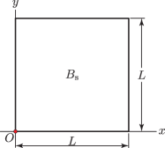
Figure 2: Domain used in the determination of convergence rates.

the domain $B_{\mathrm{s}}$ is taken to be a square of side $L=\numprint[m]{1}$. We discussed the fact that the coercivity of certain operators is strongly influenced by the volume fraction of the fluid. For this reason, we select a relatively low value of porosity to focus on this aspect. Specifically, we set the porosity in the reference configuration of the solid to be uniform and equal to 10%, which implies $\xi_{R_{\mathrm{s}}}=0.9$. We select the elastic response of the solid skeleton to be neo-Hookean (cf. Ogden, 1997) with unit shear modulus $G=\numprint[Pa]{1}$, so that, referring to the second of Eqs. (43), we have

$$\mathsf{P}^{e}=0.9\,G\,\mathsf{F}_{\mathrm{s}}.$$ (109)

The rest of the constitutive parameters are set to unit values, as indicated in Table 1.

Table 1: Summary of the parameters values in the calculation of convergence rates.

Quantity	Value
$\rho_{\mathrm{s}}^{*}$	1 $\mathrm{kg/m^{3}}$
$\rho_{\mathrm{f}}^{*}$	1 $\mathrm{kg/m^{3}}$
$\mu_{\mathrm{f}}$	1 $\mathrm{Pa\!\cdot\!s}$
$k_{\mathrm{s}}$	1 $\mathrm{m^{2}}$
$G$	1 $\mathrm{Pa}$

The analysis of the results is carried out via the Method of Manufactured Solutions (Salari and Knupp, 2000). The chosen manufactured solution is

$$\boldsymbol{u}_{\mathrm{s}} =u_{0}\sin(2\pi t/t_{0})\biggl{[}\cos\biggl{(}2\pi\frac{x+y}{L}\biggr{)}\,\hat{\imath}+\sin\biggl{(}2\pi\frac{x-y}{L}\biggr{)}\,\hat{\jmath}\biggr{]},$$ (110)

$$\boldsymbol{v}_{\mathrm{s}} =\partial_{t}\boldsymbol{u}_{\mathrm{s}},$$ (111)

$$\boldsymbol{v}_{\mathrm{f}} =v_{0}\cos(2\pi t/t_{0})\biggl{[}\sin\biggl{(}2\pi\frac{x^{2}+y^{2}}{L^{2}}\biggr{)}\,\hat{\imath}+\cos\biggl{(}2\pi\frac{x^{2}-y^{2}}{L^{2}}\biggr{)}\,\hat{\jmath}\biggr{]},$$ (112)

$$\boldsymbol{v}_{\text{flt}} =(1-\xi_{R_{\mathrm{s}}}/J_{\mathrm{s}})(\boldsymbol{v}_{\mathrm{f}}-\boldsymbol{v}_{\mathrm{s}}),$$ (113)

$$p =p_{0}\sin(2\pi t/t_{0})\sin(2\pi(x+y)/L),$$ (114)

where $u_{0}=\numprint[m]{0.01}$, $t_{0}=\numprint[s]{1}$, $v_{0}=\numprint[m/s]{1}$, $p_{0}=\numprint[Pa]{1}$, and where $J_{\mathrm{s}}=\det(\mathsf{I}+\operatorname{\nabla_{\!\boldsymbol{X}_{\mathrm{s}}}}\boldsymbol{u}_{\mathrm{s}})$.

7.1.2 Solvers and time integration

The formulations presented earlier yield time-dependent nonlinear differential-algebraic equations (DAE). We have adopted the default approach available in COMSOL Multiphysics^® for such equations. Specifically, the time-dependent aspect is implemented via the method of lines (COMSOL AB, 2015; Schiesser, 1991). The specific nonlinear solver used was IDAS (Hindmarsh et al., 2005), implementing a variable-order variable-step-size backward differentiation formulas (BDF). The solver provided by IDAS is designed to solve DAE systems of the type $F(t,y,y^{\prime},p)=0$. The BDF method was configured so as to allow orders $1$–$5$ and a maximum time step size of $\numprint[s]{0.001}$. For the linear solver we chose PARDISO 5.0.0 (Kuzmin et al., 2013; Schenk et al., 2008, 2007).

7.1.3 Finite element choice and uniform refinement setup

The triangulation over the solution’s domain $B_{\mathrm{s}_{h}}$ consisted of triangular cells. For each scalar component of the problem, the approximation spaces were piecewise Lagrange polynomials. The interpolation order was fixed to $2$ (i.e., second order Lagrange Polynomials) for all fields except the multiplier $p$. For the latter field, we have considered various interpolation orders, which will be indicated on a case by case basis and will be denoted by $\mathcal{P}^{r}_{p}$, where $r$ is the polynomial order of the interpolation.

The convergence rates were computed under uniform refinement of the solution’s domain. The uniformly refined meshes were automatically generated in COMSOL Multiphysics^® by specifying that the values of the minimum and maximum element diameter $h$ be the same. We note that the convergence rates are not uniform as a function of time, that is, they change somewhat depending on the time instant at which they are computed. With this in mind, we present results pertaining to two time instants, namely, $t=\numprint[s]{0.7}$ and $t=\numprint[s]{1.0}$. The reason for this choice is that $t=\numprint[s]{1.0}$ is the end of the time interval considered for the determination of the convergence rates, and $t=\numprint[s]{0.7}$ is representative of the worst convergence rates we have obtained in our calculations.

7.2 Fluid velocity quasi-static formulation (Problem 6) results

Here we present the results for the quasi-static stabilized formulation based on Problem 6. We note that we are not presenting results obtained with the corresponding non-stabilized formulation because we encountered severe problems in determining FE spaces of Lagrange polynomials that would produce acceptable outcomes, thus justifying the need for stabilization.

Figure 3

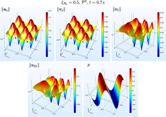
Figure 3: Fields $\|\boldsymbol{u}_{\mathrm{s}}\|$, $\|\boldsymbol{v}_{\mathrm{s}}\|$, $\|\boldsymbol{v}_{\mathrm{f}}\|$, $\|\boldsymbol{v}_{\text{flt}}\|$, and $p$ at $t=\numprint[s]{0.7}$ obtained in a calculation using the fluid velocity formulation with $\xi_{R_{\mathrm{s}}}=0.5$, and $h=(1/64)\,\mathrm{m}=\numprint[m]{0.015625}$ for a total number of degrees of freedom equal to $\numprint{187029}$.

shows the magnitude of the fields $\|\boldsymbol{u}_{\mathrm{s}}\|$, $\|\boldsymbol{v}_{\mathrm{s}}\|$, $\|\boldsymbol{v}_{\mathrm{f}}\|$, $\|\boldsymbol{v}_{\text{flt}}\|$, and $p$ at $t=\numprint[s]{0.7}$ obtained in a calculation using the stabilized fluid velocity formulation based on Problem 6 with $\xi_{R_{\mathrm{s}}}=0.5$, and $h=(1/64)\,\mathrm{m}=\numprint[m]{0.015625}$ for a total number of degrees of freedom equal to $\numprint{187029}$. The mesh used consisted of (essentially) equal size triangles with second order Lagrange polynomials for all fields. Because all convergence results presented in this paper are based on the same manufactured solution, the appearance of the plots in Fig. 3 turns out to be visually identical for all solutions regardless of formulation and order of approximation. Hence, the above plots will not be shown again for other cases.

Figures 4 and 5

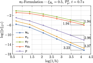
Figure 4: Convergence rates for the $L^{2}$-norm (left) and the $H^{1}$-(semi)norm (right) of the error at $t=\numprint[s]{0.7}$ obtained via the fluid velocity formulation with $\xi_{R_{\mathrm{s}}}=0.5$ and $\mathcal{P}_{p}^{2}$.

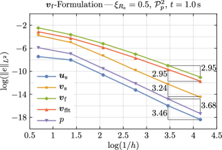
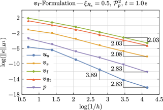
Figure 5: Convergence rates for the $L^{2}$-norm (left) and the $H^{1}$-(semi)norm (right) of the error at $t=\numprint[s]{1.0}$ obtained via the fluid velocity formulation with $\xi_{R_{\mathrm{s}}}=0.5$ and $\mathcal{P}_{p}^{2}$.

show the convergence rates for the case with $\xi_{R_{\mathrm{s}}}=0.5$ and $\mathcal{P}_{p}^{2}$ (for the other fields see Section 7.1.3) for $t=\numprint[s]{0.7}$ and $t=\numprint[s]{1.0}$, respectively. We have reported these rates both in terms of the $L^{2}$ and $H^{1}$ error norms. However, due to the formulation of the problem, there is no set expectation on the convergence rates of the $H^{1}$ norm for the fields $\boldsymbol{v}_{\mathrm{f}}$ and $\boldsymbol{v}_{\text{flt}}$. As far as the values of the convergence rates are concerned, we refer to the results for the time-independent linear Darcy-flow problem through a rigid porous medium presented by Masud and Hughes (2002). We note that the velocity field in the cited work corresponds to the filtration velocity in the present paper. With this in mind, Masud and Hughes (2002) found that for $k_{\mathrm{s}}/\mu=1$, and for continuous pressure $6$-node triangles and continuous pressure $9$-node quadrilaterals the convergence rates in terms of the $L^{2}$-norm of $\boldsymbol{v}_{\text{flt}}$ approached the optimal value of $2$, and the $L^{2}$- and $H^{1}$-norms of $p$ approached the optimal value of $3$ and $2$, respectively (cf. Fig. 17 in Masud and Hughes, 2002). With reference to Figs. 4 and 5, as well as Tables 2 and 3,

Table 2: Convergence rates for the stabilized fluid velocity formulation for $t=\numprint[s]{0.7}$ with $\xi_{R_{\mathrm{s}}}=0.5$ and$\mathcal{P}_{p}^{2}$ corresponding to Fig. 4.

$h$ (m)	$\|\boldsymbol{u}_{\mathrm{s}}\|_{L^{2}}$	$\|\boldsymbol{v}_{\mathrm{s}}\|_{L^{2}}$	$\|\boldsymbol{v}_{\mathrm{f}}\|_{L^{2}}$	$\|\boldsymbol{v}_{\text{flt}}\|_{L^{2}}$	$\|p\|_{L^{2}}$	$\|\boldsymbol{u}_{\mathrm{s}}\|_{H^{1}}$	$\|\boldsymbol{v}_{\mathrm{s}}\|_{H^{1}}$	$\|p\|_{H^{1}}$
$\tfrac{1}{2}\to\tfrac{1}{4}$	$-1.84$	$-1.95$	$-0.567$	$-0.624$	$-1.90$	$-1.34$	$-1.52$	$-0.372$
$\tfrac{1}{4}\to\tfrac{1}{8}$	$-3.33$	$-3.62$	$-1.35$	$-1.34$	$-2.63$	$-2.18$	$-2.33$	$-1.84$
$\tfrac{1}{8}\to\tfrac{1}{16}$	$-3.64$	$-3.66$	$-1.68$	$-1.68$	$-2.92$	$-2.38$	$-2.41$	$-2.03$
$\tfrac{1}{16}\to\tfrac{1}{32}$	$-3.46$	$-3.57$	$-1.84$	$-1.84$	$-2.93$	$-2.21$	$-2.21$	$-2.00$
$\tfrac{1}{32}\to\tfrac{1}{64}$	$-3.23$	$-3.37$	$-1.94$	$-1.94$	$-2.96$	$-2.08$	$-2.08$	$-1.99$

Table 3: Convergence rates for the stabilized fluid velocity formulation for $t=\numprint[s]{1.0}$ with $\xi_{R_{\mathrm{s}}}=0.5$ and$\mathcal{P}_{p}^{2}$ corresponding to Fig. 5.

$h$ (m)	$\|\boldsymbol{u}_{\mathrm{s}}\|_{L^{2}}$	$\|\boldsymbol{v}_{\mathrm{s}}\|_{L^{2}}$	$\|\boldsymbol{v}_{\mathrm{f}}\|_{L^{2}}$	$\|\boldsymbol{v}_{\text{flt}}\|_{L^{2}}$	$\|p\|_{L^{2}}$	$\|\boldsymbol{u}_{\mathrm{s}}\|_{H^{1}}$	$\|\boldsymbol{v}_{\mathrm{s}}\|_{H^{1}}$	$\|p\|_{H^{1}}$
$\tfrac{1}{2}\to\tfrac{1}{4}$	$-0.835$	$-1.75$	$-1.68$	$-1.60$	$-1.53$	$-1.13$	$-1.31$	$-2.21$
$\tfrac{1}{4}\to\tfrac{1}{8}$	$-3.77$	$-3.37$	$-2.26$	$-2.34$	$-3.73$	$-3.64$	$-2.18$	$-2.68$
$\tfrac{1}{8}\to\tfrac{1}{16}$	$-3.78$	$-3.65$	$-2.63$	$-2.64$	$-3.74$	$-3.78$	$-2.38$	$-2.32$
$\tfrac{1}{16}\to\tfrac{1}{32}$	$-3.95$	$-3.47$	$-2.86$	$-2.87$	$-3.88$	$-3.89$	$-2.20$	$-2.60$
$\tfrac{1}{32}\to\tfrac{1}{64}$	$-3.46$	$-3.24$	$-2.95$	$-2.95$	$-3.68$	$-2.83$	$-2.08$	$-2.83$

our results for the “worst-case” scenario ($t=\numprint[s]{0.7}$) behave in a way consistent with results in Masud and Hughes (2002) and exceed expectations (with respect to the linear problem) for other time instants. In Tables 2 and 3, we have omitted $H^{1}$ error norm results for $\boldsymbol{v}_{\mathrm{f}}$ and $\boldsymbol{v}_{\text{flt}}$ since no formal results exist for these fields. As far as the solid displacement and velocity fields are concerned, we have found results that consistently exceed expectations relative to typical estimates for linear elasto-statics and we have often run into somewhat puzzling super-convergent behavior as that shown in Fig. 5.

Figures 6 and 7

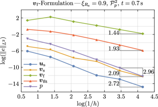
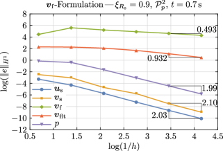
Figure 6: Convergence rates for the $L^{2}$-norm (left) and the $H^{1}$-(semi)norm (right) of the error at $t=\numprint[s]{0.7}$ obtained via the fluid velocity formulation with $\xi_{R_{\mathrm{s}}}=0.9$ and $\mathcal{P}_{p}^{2}$.

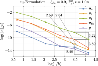
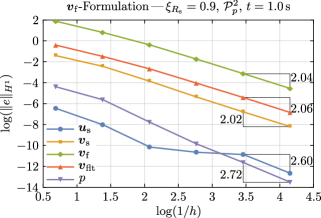
Figure 7: Convergence rates for the $L^{2}$-norm (left) and the $H^{1}$-(semi)norm (right) of the error at $t=\numprint[s]{1.0}$ obtained via the fluid velocity formulation with $\xi_{R_{\mathrm{s}}}=0.9$ and $\mathcal{P}_{p}^{2}$.

as well as Tables 4 and 5

Table 4: Convergence rates for the stabilized fluid velocity formulation for $t=\numprint[s]{0.7}$ with $\xi_{R_{\mathrm{s}}}=0.9$ and$\mathcal{P}_{p}^{2}$ corresponding to Fig. 6.

$h$ (m)	$\|\boldsymbol{u}_{\mathrm{s}}\|_{L^{2}}$	$\|\boldsymbol{v}_{\mathrm{s}}\|_{L^{2}}$	$\|\boldsymbol{v}_{\mathrm{f}}\|_{L^{2}}$	$\|\boldsymbol{v}_{\text{flt}}\|_{L^{2}}$	$\|p\|_{L^{2}}$	$\|\boldsymbol{u}_{\mathrm{s}}\|_{H^{1}}$	$\|\boldsymbol{v}_{\mathrm{s}}\|_{H^{1}}$	$\|p\|_{H^{1}}$
$\tfrac{1}{2}\to\tfrac{1}{4}$	$-2.05$	$-1.16$	$1.20$	$-0.693$	$-1.89$	$-1.48$	$-0.808$	$-0.363$
$\tfrac{1}{4}\to\tfrac{1}{8}$	$-3.22$	$-2.87$	$-1.64$	$-1.31$	$-2.56$	$-2.06$	$-2.42$	$-1.82$
$\tfrac{1}{8}\to\tfrac{1}{16}$	$-3.23$	$-1.28$	$-1.38$	$-1.66$	$-2.91$	$-2.18$	$-1.54$	$-2.03$
$\tfrac{1}{16}\to\tfrac{1}{32}$	$-1.36$	$-3.26$	$-1.43$	$-1.83$	$-2.91$	$-2.06$	$-2.52$	$-2.00$
$\tfrac{1}{32}\to\tfrac{1}{64}$	$-2.72$	$-2.09$	$-1.44$	$-1.93$	$-2.96$	$-2.03$	$-2.10$	$-1.99$

Table 5: Convergence rates for the stabilized fluid velocity formulation for $t=\numprint[s]{1.0}$ with $\xi_{R_{\mathrm{s}}}=0.9$ and$\mathcal{P}_{p}^{2}$ corresponding to Fig. 7.

$h$ (m)	$\|\boldsymbol{u}_{\mathrm{s}}\|_{L^{2}}$	$\|\boldsymbol{v}_{\mathrm{s}}\|_{L^{2}}$	$\|\boldsymbol{v}_{\mathrm{f}}\|_{L^{2}}$	$\|\boldsymbol{v}_{\text{flt}}\|_{L^{2}}$	$\|p\|_{L^{2}}$	$\|\boldsymbol{u}_{\mathrm{s}}\|_{H^{1}}$	$\|\boldsymbol{v}_{\mathrm{s}}\|_{H^{1}}$	$\|p\|_{H^{1}}$
$\tfrac{1}{2}\to\tfrac{1}{4}$	$-2.68$	$-1.98$	$-1.70$	$-1.71$	$-2.60$	$-2.26$	$-1.48$	$-1.79$
$\tfrac{1}{4}\to\tfrac{1}{8}$	$-2.82$	$-3.21$	$-2.63$	$-2.68$	$-3.11$	$-3.07$	$-2.05$	$-3.10$
$\tfrac{1}{8}\to\tfrac{1}{16}$	$-1.22$	$-3.45$	$-2.73$	$-2.78$	$-3.60$	$-0.715$	$-2.18$	$-3.00$
$\tfrac{1}{16}\to\tfrac{1}{32}$	$-0.381$	$-2.69$	$-1.92$	$-1.83$	$-1.34$	$-0.314$	$-2.06$	$-2.57$
$\tfrac{1}{32}\to\tfrac{1}{64}$	$-2.59$	$-2.64$	$-3.22$	$-3.89$	$-2.48$	$-2.60$	$-2.02$	$-2.72$

show the convergence rates for the case with $\xi_{R_{\mathrm{s}}}=0.9$, that is, for high concentration of the solid phase. As can be seen, several of the observations made for the case with $\xi_{R_{\mathrm{s}}}=0.5$ still apply. However, it is apparent that the convergence rates are more erratic and have degraded. The degradation of the convergence rates was expected in that the volume fraction $\xi_{R_{\mathrm{s}}}$ appears as a coefficient affecting the coercivity of some operators and it affects limit behaviors as the values $0$ and $1$ are approached. To gather some information about the formulation’s behavior as a function of $\xi_{R_{\mathrm{s}}}$, we have conducted a parametric sweep with $0.25\leq\xi_{R_{\mathrm{s}}}\leq 0.95$. This calculation was carried out with $h=(1/32)\,\mathrm{m}$ and the results are shown in Figs. 8 and 9.

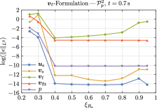
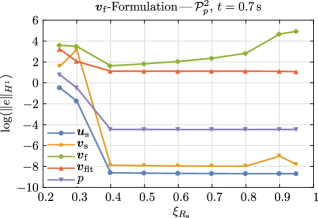
Figure 8: $L^{2}$-norm (left) and the $H^{1}$-(semi)norm (right) of the error at $t=\numprint[s]{0.7}$ for the fluid velocity formulation as a function of $\xi_{R_{\mathrm{s}}}$. The element diameter for this simulation was $h=(1/32)\,\mathrm{m}$.

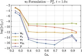
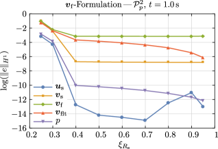
Figure 9: $L^{2}$-norm (left) and the $H^{1}$-(semi)norm (right) of the error at $t=\numprint[s]{1.0}$ for the fluid velocity formulation as a function of $\xi_{R_{\mathrm{s}}}$. The element diameter for this simulation was $h=(1/32)\,\mathrm{m}$.

These results indicate that the accuracy is highly degraded for all fields for high volume fractions of the fluid. From a numerical viewpoint, a different formulation would be needed for these cases. More importantly, from a physical viewpoint, cases with high porosity, i.e., high fluid volume fractions, should be modeled as Brinkman flow problems (cf. Masud, 2007). For increasing values of $\xi_{R_{\mathrm{s}}}$, Fig. 8 and 9 show degraded accuracy for the field $\boldsymbol{v}_{\mathrm{f}}$, while the accuracy in terms of the other fields, especially $\boldsymbol{v}_{\text{flt}}$ and $p$, appears to be relatively unaffected by increasing values of the solid volume fraction.

For the stabilized quasi-static formulation there are no restrictions induced by the Brezzi-Babuška condition. To illustrate this point, in Figs. 10 and 11

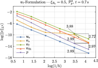
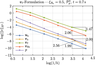
Figure 10: Convergence rates for the $L^{2}$-norm (left) and the $H^{1}$-(semi)norm (right) of the error at $t=\numprint[s]{0.7}$ obtained via the fluid velocity formulation with $\xi_{R_{\mathrm{s}}}=0.5$ and $\mathcal{P}_{p}^{3}$.

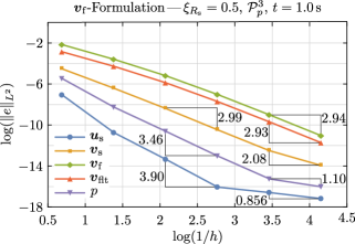
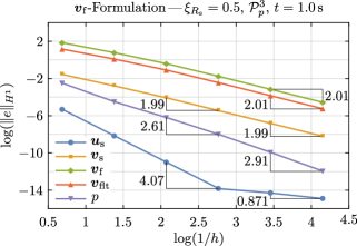
Figure 11: Convergence rates for the $L^{2}$-norm (left) and the $H^{1}$-(semi)norm (right) of the error at $t=\numprint[s]{1.0}$ obtained via the fluid velocity formulation with $\xi_{R_{\mathrm{s}}}=0.5$ and $\mathcal{P}_{p}^{3}$.

we present results with $\xi_{R_{\mathrm{s}}}=0.5$ in which all fields are interpolated via second order Lagrange polynomials except $p$, which is interpolated using cubic Lagrange polynomials. In addition to illustrating the possibility of choosing arbitrary solution spaces, the result in question reveals an interesting effect. While the observed convergence rates are not easily explained and require a formal analysis, it appears that by increasing the order of interpolation of $p$ has a beneficial effect on the order of convergence of of the fields $\boldsymbol{v}_{\mathrm{f}}$ and $\boldsymbol{v}_{\text{flt}}$ without negatively affecting the behavior of the fields $\boldsymbol{u}_{\mathrm{s}}$ and $\boldsymbol{v}_{\mathrm{s}}$ (in fact, somewhat positive). If confirmed, this result suggests that one might gain almost a full order of convergence in the vector fields $\boldsymbol{v}_{\mathrm{f}}$ and $\boldsymbol{v}_{\text{flt}}$ at the relatively moderate cost of increasing the degrees of freedom of a scalar field.

7.3 Filtration velocity quasi-static formulation (Problem 9) results

The convergence results for the quasi-static problem solved using the stabilized filtration velocity formulation in Problem 9 for $\xi_{R_{\mathrm{s}}}=0.5$ are presented in Figs. 12 and 13.

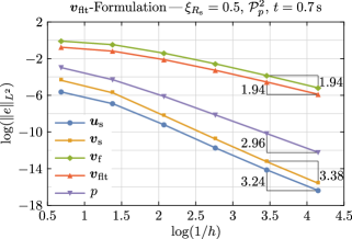
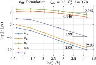
Figure 12: Convergence rates for the $L^{2}$-norm (left) and the $H^{1}$-(semi)norm (right) of the error at $t=\numprint[s]{0.7}$ obtained via the filtration velocity formulation with $\xi_{R_{\mathrm{s}}}=0.5$ and $\mathcal{P}_{p}^{2}$.

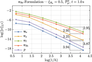
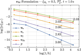
Figure 13: Convergence rates for the $L^{2}$-norm (left) and the $H^{1}$-(semi)norm (right) of the error at $t=\numprint[s]{1.0}$ obtained via the filtration velocity formulation with $\xi_{R_{\mathrm{s}}}=0.5$ and $\mathcal{P}_{p}^{2}$.

The detailed convergence rates corresponding to Figs. 12 and 13 are in Tables 6 and 7.

Table 6: Convergence rates for the stabilized filtration velocity formulation for $t=\numprint[s]{0.7}$ with $\xi_{R_{\mathrm{s}}}=0.5$ and$\mathcal{P}_{p}^{2}$ corresponding to Fig. 12.

$h$ (m)	$\|\boldsymbol{u}_{\mathrm{s}}\|_{L^{2}}$	$\|\boldsymbol{v}_{\mathrm{s}}\|_{L^{2}}$	$\|\boldsymbol{v}_{\mathrm{f}}\|_{L^{2}}$	$\|\boldsymbol{v}_{\text{flt}}\|_{L^{2}}$	$\|p\|_{L^{2}}$	$\|\boldsymbol{u}_{\mathrm{s}}\|_{H^{1}}$	$\|\boldsymbol{v}_{\mathrm{s}}\|_{H^{1}}$	$\|p\|_{H^{1}}$
$\tfrac{1}{2}\to\tfrac{1}{4}$	$-1.85$	$-1.96$	$-0.559$	$-0.613$	$-1.90$	$-1.33$	$-1.52$	$-0.375$
$\tfrac{1}{4}\to\tfrac{1}{8}$	$-3.33$	$-3.62$	$-1.35$	$-1.35$	$-2.63$	$-2.19$	$-2.34$	$-1.84$
$\tfrac{1}{8}\to\tfrac{1}{16}$	$-3.64$	$-3.67$	$-1.68$	$-1.68$	$-2.92$	$-2.38$	$-2.41$	$-2.03$
$\tfrac{1}{16}\to\tfrac{1}{32}$	$-3.46$	$-3.57$	$-1.84$	$-1.84$	$-2.93$	$-2.21$	$-2.21$	$-2.00$
$\tfrac{1}{32}\to\tfrac{1}{64}$	$-3.24$	$-3.38$	$-1.94$	$-1.94$	$-2.96$	$-2.08$	$-2.08$	$-1.99$

Table 7: Convergence rates for the stabilized filtration velocity formulation for $t=\numprint[s]{1.0}$ with $\xi_{R_{\mathrm{s}}}=0.5$ and$\mathcal{P}_{p}^{2}$ corresponding to Fig. 13.

$h$ (m)	$\|\boldsymbol{u}_{\mathrm{s}}\|_{L^{2}}$	$\|\boldsymbol{v}_{\mathrm{s}}\|_{L^{2}}$	$\|\boldsymbol{v}_{\mathrm{f}}\|_{L^{2}}$	$\|\boldsymbol{v}_{\text{flt}}\|_{L^{2}}$	$\|p\|_{L^{2}}$	$\|\boldsymbol{u}_{\mathrm{s}}\|_{H^{1}}$	$\|\boldsymbol{v}_{\mathrm{s}}\|_{H^{1}}$	$\|p\|_{H^{1}}$
$\tfrac{1}{2}\to\tfrac{1}{4}$	$-0.865$	$-1.76$	$-1.68$	$-1.60$	$-1.53$	$-1.14$	$-1.31$	$-2.20$
$\tfrac{1}{4}\to\tfrac{1}{8}$	$-3.81$	$-3.38$	$-2.26$	$-2.34$	$-3.77$	$-3.68$	$-2.18$	$-2.69$
$\tfrac{1}{8}\to\tfrac{1}{16}$	$-3.76$	$-3.65$	$-2.63$	$-2.64$	$-3.73$	$-3.76$	$-2.38$	$-2.31$
$\tfrac{1}{16}\to\tfrac{1}{32}$	$-3.93$	$-3.47$	$-2.86$	$-2.87$	$-3.88$	$-3.90$	$-2.20$	$-2.60$
$\tfrac{1}{32}\to\tfrac{1}{64}$	$-3.94$	$-3.25$	$-2.95$	$-2.95$	$-3.87$	$-3.68$	$-2.08$	$-2.83$

These results are virtually identical to those already presented in Figs 4 and 5 indicating that for $\xi_{R_{\mathrm{s}}}=0.5$ there is no appreciable difference between the two formulations. Hence, we can say that the convergence rates approach optimal values in the sense discussed earlier.

The convergence results for the quasi-static problem solved using the stabilized filtration velocity formulation in Problem 9 for $\xi_{R_{\mathrm{s}}}=0.9$ are presented in Figs. 14 and 15.

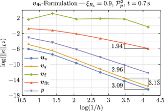
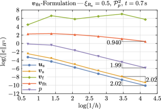
Figure 14: Convergence rates for the $L^{2}$-norm (left) and the $H^{1}$-(semi)norm (right) of the error at $t=\numprint[s]{0.7}$ obtained via the filtration velocity formulation with $\xi_{R_{\mathrm{s}}}=0.9$ and $\mathcal{P}_{p}^{2}$. The rates for $\boldsymbol{v}_{\mathrm{f}}$ have been omitted.

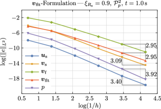
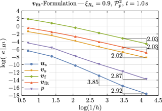
Figure 15: Convergence rates for the $L^{2}$-norm (left) and the $H^{1}$-(semi)norm (right) of the error at $t=\numprint[s]{1.0}$ obtained via the filtration velocity formulation with $\xi_{R_{\mathrm{s}}}=0.9$ and $\mathcal{P}_{p}^{2}$. The rates for $\boldsymbol{v}_{\mathrm{f}}$ have been omitted.

The results in Figs. 14 and 15 present a slight improvement in the behavior of the fields $\boldsymbol{u}_{\mathrm{s}}$, $\boldsymbol{v}_{\mathrm{f}}$, $\boldsymbol{v}_{\text{flt}}$, and $p$ relative to that of the fluid velocity formulation (Figs. 6 and 7). However, for the plots with $t=\numprint[s]{0.7}$, the behavior in the field $\boldsymbol{v}_{\mathrm{f}}$ is degraded to the point that non-convergent behavior can be clearly observed. This result suggests that the filtration velocity formulation does not have clear advantages over the fluid velocity formulation in terms of accuracy and reliability, at least for the parameter set and range of $\xi_{R_{\mathrm{s}}}$ used in this paper.

8 Conclusions

In this paper we considered the quasi-static motion of a poroelastic system consisting of an hyperelastic incompressible solid skeleton saturated by an incompressible viscous fluid. The model considered stems from mixture theory and it is intended for modular expansion to include progressively more complex physics such as the chemistry of biodegradation. For this system, we considered a consistent stabilized FEM predicated on the assumption that the porosity data provided as input to the model is not necessarily smooth. For said formulation we proved stability and obtained convergence rates using the method of manufactured solutions. We have shown that the rates in question are optimal relative to the estimates by Masud and Hughes (2002) and that in some cases, supercovergence is observed. Future work will focus on the formulation of a stable FEM that includes inertia effects.

Appendix

Operators in the dual formulation

This Appendix presents the definitions of the operators used in defining the dual formulation introduced earlier in the paper. Following Heltai and Costanzo (2012), we introduce the following notation

$$\prescript{}{V^{*}}{\bigl{\langle}}\psi,\phi\big{\rangle}_{V},$$ (115)

in which, given a vector space $V$ and its dual $V^{*}$, $\psi$ and $\phi$ are elements of the vector spaces $V^{*}$ and $V$, respectively, and where $\prescript{}{V^{*}}{\bigl{\langle}}\bullet,\bullet\big{\rangle}_{V}$ identifies the duality product between $V^{*}$ and $V$. , The operators defined in this Appendix, although not all linear, can be interpreted as though they were matrices. For this reason we adopt the following notation to identify the domain and ranges of the operators in question and whether or not they are linear:

• We will refer to the spaces $\mathcal{V}^{\boldsymbol{u}_{\mathrm{s}}}$, $\mathcal{V}^{\boldsymbol{v}_{\mathrm{s}}}$, $\mathcal{V}^{\boldsymbol{v}_{\mathrm{f}}}$, and $\mathcal{V}^{p}$ are identified by the indices $1$, $2$, $3$, and $4$, respectively.

• We will refer to the spaces $(\mathcal{V}^{\boldsymbol{u}_{\mathrm{s}}})^{*}$, $(\mathcal{V}^{\boldsymbol{v}_{\mathrm{s}}})^{*}$, $(\mathcal{V}^{\boldsymbol{v}_{\mathrm{f}}})^{*}$, and $(\mathcal{V}^{p})^{*}$ are identified by the indices $\bar{1}$, $\bar{2}$, $\bar{3}$, and $\bar{4}$, respectively.

• If an operator is nonlinear, the symbol denoting the operator will be followed by a list in parenthesis containing the fields on which the operator depends. If the list is absent, then the operator is understood to be linear.

• If an operator is characterized by one one subscript, the latter denotes the range of the operator.

For example, the notation $\mathcal{M}_{\bar{1}1}$ denotes a linear operator mapping an element $\mathcal{V}^{\boldsymbol{u}_{\mathrm{s}}}$ into an element of $(\mathcal{V}^{\boldsymbol{u}_{\mathrm{s}}})^{*}$. By contrast, an operator $\mathcal{A}_{\bar{2}3}(\boldsymbol{u}_{\mathrm{s}})$ denotes a nonlinear operator that depends on $\boldsymbol{u}_{\mathrm{s}}$ and that maps an element of $\mathcal{V}^{\boldsymbol{v}_{\mathrm{f}}}$ into an element of $(\mathcal{V}^{\boldsymbol{v}_{\mathrm{s}}})^{*}$. As a final example, an operator denoted by $\mathcal{F}_{2}(\boldsymbol{u}_{\mathrm{s}})$ is an operator that depends on $\boldsymbol{u}_{\mathrm{s}}$ and takes values in $\mathcal{V}^{\boldsymbol{v}_{\mathrm{s}}}$.

Operators used to define Problem 5

With the above in mind, we define the following operators:

$$\mathcal{M}_{\bar{1}1} :\mathcal{H}^{\boldsymbol{u}_{\mathrm{s}}}\to(\mathcal{V}^{\boldsymbol{u}_{\mathrm{s}}})^{*}, \quad\prescript{}{(\mathcal{V}^{\boldsymbol{u}_{\mathrm{s}}})^{*}}{\bigl{\langle}}\mathcal{M}_{\bar{1}1}\boldsymbol{v},\boldsymbol{w}\big{\rangle}_{\mathcal{V}^{\boldsymbol{u}_{\mathrm{s}}}} \coloneqq\int_{B_{\mathrm{s}}}\boldsymbol{w}\cdot\boldsymbol{v},$$

$$\qquad\qquad\forall\boldsymbol{v}\in\mathcal{H}^{\boldsymbol{u}_{\mathrm{s}}},\forall\boldsymbol{w}\in\mathcal{V}^{\boldsymbol{u}_{\mathrm{s}}}_{0},$$ (116)

$$\mathcal{M}_{\bar{1}2} :\mathcal{V}^{\boldsymbol{v}_{\mathrm{s}}}\to(\mathcal{V}^{\boldsymbol{u}_{\mathrm{s}}})^{*}, \quad\prescript{}{(\mathcal{V}^{\boldsymbol{u}_{\mathrm{s}}})^{*}}{\bigl{\langle}}\mathcal{M}_{\bar{1}2}\boldsymbol{v},\boldsymbol{w}\big{\rangle}_{\mathcal{V}^{\boldsymbol{u}_{\mathrm{s}}}} \coloneqq\int_{B_{\mathrm{s}}}\boldsymbol{w}\cdot\boldsymbol{v},$$

$$\qquad\qquad\forall\boldsymbol{v}\in\mathcal{V}^{\boldsymbol{v}_{\mathrm{s}}},\forall\boldsymbol{w}\in\mathcal{V}^{\boldsymbol{u}_{\mathrm{s}}}_{0},$$ (117)

$$\mathcal{B}_{\bar{4}2}(\boldsymbol{u}_{\mathrm{s}};\xi_{R_{\mathrm{s}}}) :\mathcal{V}^{\boldsymbol{v}_{\mathrm{s}}}\to(\mathcal{V}^{p})^{*}, \quad\prescript{}{(\mathcal{V}^{p})^{*}}{\bigl{\langle}}\mathcal{B}_{\bar{4}2}(\boldsymbol{u}_{\mathrm{s}};\xi_{R_{\mathrm{s}}})\boldsymbol{v},q\big{\rangle}_{\mathcal{V}^{p}} \coloneqq-\int_{B_{\mathrm{s}}}\xi_{R_{\mathrm{s}}}\operatorname{\nabla_{\!\boldsymbol{X}_{\mathrm{s}}}}q\cdot\mathsf{F}_{\mathrm{s}}^{-1}\boldsymbol{v},$$

$$\qquad\qquad\forall\boldsymbol{v}\in\mathcal{V}^{\boldsymbol{v}_{\mathrm{s}}},\forall q\in\mathcal{V}^{p},$$ (118)

$$\mathcal{B}^{\mathrm{T}}_{\bar{4}2}(\boldsymbol{u}_{\mathrm{s}};\xi_{R_{\mathrm{s}}}) :\mathcal{V}^{p}\to(\mathcal{V}^{\boldsymbol{v}_{\mathrm{s}}})^{*}, \quad\prescript{}{(\mathcal{V}^{\boldsymbol{v}_{\mathrm{s}}})^{*}}{\bigl{\langle}}\mathcal{B}^{\mathrm{T}}_{\bar{4}2}(\boldsymbol{u}_{\mathrm{s}};\xi_{R_{\mathrm{s}}})q,\boldsymbol{v}\big{\rangle}_{\mathcal{V}^{\boldsymbol{v}_{\mathrm{s}}}} \coloneqq-\int_{B_{\mathrm{s}}}\xi_{R_{\mathrm{s}}}\operatorname{\nabla_{\!\boldsymbol{X}_{\mathrm{s}}}}q\cdot\mathsf{F}_{\mathrm{s}}^{-1}\boldsymbol{v},$$

$$\qquad\qquad\forall q\in\mathcal{V}^{p},\forall\boldsymbol{v}\in\mathcal{V}^{\boldsymbol{v}_{\mathrm{s}}}_{0},$$ (119)

$$\mathcal{B}_{\bar{4}3}(\boldsymbol{u}_{\mathrm{s}};\xi_{R_{\mathrm{s}}}) :\mathcal{V}^{\boldsymbol{v}_{\mathrm{f}}}\to(\mathcal{V}^{p})^{*}, \quad\prescript{}{(\mathcal{V}^{p})^{*}}{\bigl{\langle}}\mathcal{B}_{\bar{4}3}(\boldsymbol{u}_{\mathrm{s}};\xi_{R_{\mathrm{s}}})\boldsymbol{v},q\big{\rangle}_{\mathcal{V}^{p}} \coloneqq-\int_{B_{\mathrm{s}}}(J_{\mathrm{s}}-\xi_{R_{\mathrm{s}}})\operatorname{\nabla_{\!\boldsymbol{X}_{\mathrm{s}}}}q\cdot\mathsf{F}_{\mathrm{s}}^{-1}\boldsymbol{v},$$

$$\qquad\qquad\forall\boldsymbol{v}\in\mathcal{V}^{\boldsymbol{v}_{\mathrm{f}}},\forall q\in\mathcal{V}^{p},$$ (120)

$$\mathcal{B}^{\mathrm{T}}_{\bar{4}3}(\boldsymbol{u}_{\mathrm{s}};\xi_{R_{\mathrm{s}}}) :\mathcal{V}^{p}\to(\mathcal{V}^{\boldsymbol{v}_{\mathrm{f}}})^{*}, \quad\prescript{}{(\mathcal{V}^{\boldsymbol{v}_{\mathrm{f}}})^{*}}{\bigl{\langle}}\mathcal{B}^{\mathrm{T}}_{\bar{4}3}(\boldsymbol{u}_{\mathrm{s}};\xi_{R_{\mathrm{s}}})q,\boldsymbol{v}\big{\rangle}_{\mathcal{V}^{\boldsymbol{v}_{\mathrm{f}}}} \coloneqq-\int_{B_{\mathrm{s}}}(J_{\mathrm{s}}-\xi_{R_{\mathrm{s}}})\operatorname{\nabla_{\!\boldsymbol{X}_{\mathrm{s}}}}q\cdot\mathsf{F}_{\mathrm{s}}^{-1}\boldsymbol{v},$$

$$\qquad\qquad\forall q\in\mathcal{V}^{p},\forall\boldsymbol{v}\in\mathcal{V}^{\boldsymbol{v}_{\mathrm{f}}},$$ (121)

$$\mathcal{M}_{\bar{3}3}(\boldsymbol{u}_{\mathrm{s}};\xi_{R_{\mathrm{s}}}) :\mathcal{H}^{\boldsymbol{v}_{\mathrm{f}}}\to(\mathcal{V}^{\boldsymbol{v}_{\mathrm{f}}})^{*}, \quad\prescript{}{(\mathcal{V}^{\boldsymbol{v}_{\mathrm{f}}})^{*}}{\bigl{\langle}}\mathcal{M}_{\bar{3}3}(\boldsymbol{u}_{\mathrm{s}};\xi_{R_{\mathrm{s}}})\boldsymbol{w},\boldsymbol{v}\big{\rangle}_{\mathcal{V}^{\boldsymbol{v}_{\mathrm{f}}}} \coloneqq\int_{B_{\mathrm{s}}}(J_{\mathrm{s}}-\xi_{R_{\mathrm{s}}})\rho^{*}_{\mathrm{f}}\boldsymbol{w}\cdot\boldsymbol{v},$$

$$\qquad\qquad\forall\boldsymbol{w}\in\mathcal{H}^{\boldsymbol{v}_{\mathrm{f}}},\forall\boldsymbol{v}\in\mathcal{V}^{\boldsymbol{v}_{\mathrm{f}}},$$ (122)

$$\mathcal{N}_{\bar{3}3}(\boldsymbol{u}_{\mathrm{s}},\boldsymbol{v}_{\mathrm{f}};\xi_{R_{\mathrm{s}}}) :\mathcal{V}^{\boldsymbol{v}_{\mathrm{f}}}\to(\mathcal{V}^{\boldsymbol{v}_{\mathrm{f}}})^{*}, \begin{aligned} &\prescript{}{(\mathcal{V}^{\boldsymbol{v}_{\mathrm{f}}})^{*}}{\bigl{\langle}}\mathcal{N}_{\bar{3}3}(\boldsymbol{u}_{\mathrm{s}},\boldsymbol{v}_{\mathrm{f}};\xi_{R_{\mathrm{s}}})\boldsymbol{w},\boldsymbol{v}\big{\rangle}_{\mathcal{V}^{\boldsymbol{v}_{\mathrm{f}}}}\\ &\hskip 99.58464pt\coloneqq\int_{B_{\mathrm{s}}}(J_{\mathrm{s}}-\xi_{R_{\mathrm{s}}})\rho^{*}_{\mathrm{f}}\operatorname{\nabla_{\!\boldsymbol{X}_{\mathrm{s}}}}\boldsymbol{v}_{\mathrm{f}}\mathsf{F}_{\mathrm{s}}^{-1}\boldsymbol{w}\cdot\boldsymbol{v},\end{aligned}$$

$$\qquad\qquad\qquad\forall\boldsymbol{w},\boldsymbol{v}\in\mathcal{V}^{\boldsymbol{v}_{\mathrm{f}}},$$ (123)

$$\mathcal{N}_{\bar{3}2}(\boldsymbol{u}_{\mathrm{s}},\boldsymbol{v}_{\mathrm{f}};\xi_{R_{\mathrm{s}}}) :\mathcal{V}^{\boldsymbol{v}_{\mathrm{s}}}\to(\mathcal{V}^{\boldsymbol{v}_{\mathrm{f}}})^{*}, \begin{aligned} &\prescript{}{(\mathcal{V}^{\boldsymbol{v}_{\mathrm{f}}})^{*}}{\bigl{\langle}}\mathcal{N}_{\bar{3}2}(\boldsymbol{u}_{\mathrm{s}},\boldsymbol{v}_{\mathrm{f}};\xi_{R_{\mathrm{s}}})\boldsymbol{w},\boldsymbol{v}\big{\rangle}_{\mathcal{V}^{\boldsymbol{v}_{\mathrm{f}}}}\\ &\hskip 99.58464pt\coloneqq\int_{B_{\mathrm{s}}}(J_{\mathrm{s}}-\xi_{R_{\mathrm{s}}})\rho^{*}_{\mathrm{f}}\operatorname{\nabla_{\!\boldsymbol{X}_{\mathrm{s}}}}\boldsymbol{v}_{\mathrm{f}}\mathsf{F}_{\mathrm{s}}^{-1}\boldsymbol{w}\cdot\boldsymbol{v},\end{aligned}$$

$$\qquad\qquad\forall\boldsymbol{w}\in\mathcal{V}^{\boldsymbol{v}_{\mathrm{s}}},\forall\boldsymbol{v}\in\mathcal{V}^{\boldsymbol{v}_{\mathrm{f}}},$$ (124)

$$\mathcal{D}_{\bar{3}3}(\boldsymbol{u}_{\mathrm{s}};\xi_{R_{\mathrm{s}}}) :\mathcal{V}^{\boldsymbol{v}_{\mathrm{f}}}\to(\mathcal{V}^{\boldsymbol{v}_{\mathrm{f}}})^{*}, \quad\prescript{}{(\mathcal{V}^{\boldsymbol{v}_{\mathrm{f}}})^{*}}{\bigl{\langle}}\mathcal{D}_{\bar{3}3}(\boldsymbol{u}_{\mathrm{s}};\xi_{R_{\mathrm{s}}})\boldsymbol{w},\boldsymbol{v}\big{\rangle}_{\mathcal{V}^{\boldsymbol{v}_{\mathrm{f}}}} \coloneqq\int_{B_{\mathrm{s}}}(J_{\mathrm{s}}-\xi_{R_{\mathrm{s}}})^{2}\frac{\mu_{\mathrm{f}}}{J_{\mathrm{s}}k_{\mathrm{s}}}\boldsymbol{w}\cdot\boldsymbol{v},$$

$$\qquad\qquad\forall\boldsymbol{w},\boldsymbol{v}\in\mathcal{V}^{\boldsymbol{v}_{\mathrm{f}}},$$ (125)

$$\mathcal{D}_{\bar{3}2}(\boldsymbol{u}_{\mathrm{s}};\xi_{R_{\mathrm{s}}}) :\mathcal{V}^{\boldsymbol{v}_{\mathrm{s}}}\to(\mathcal{V}^{\boldsymbol{v}_{\mathrm{f}}})^{*}, \quad\prescript{}{(\mathcal{V}^{\boldsymbol{v}_{\mathrm{f}}})^{*}}{\bigl{\langle}}\mathcal{D}_{\bar{3}2}(\boldsymbol{u}_{\mathrm{s}};\xi_{R_{\mathrm{s}}})\boldsymbol{w},\boldsymbol{v}\big{\rangle}_{\mathcal{V}^{\boldsymbol{v}_{\mathrm{f}}}} \coloneqq\int_{B_{\mathrm{s}}}(J_{\mathrm{s}}-\xi_{R_{\mathrm{s}}})^{2}\frac{\mu_{\mathrm{f}}}{J_{\mathrm{s}}k_{\mathrm{s}}}\boldsymbol{w}\cdot\boldsymbol{v},$$

$$\qquad\qquad\forall\boldsymbol{w}\in\mathcal{V}^{\boldsymbol{v}_{\mathrm{s}}},\forall\boldsymbol{v}\in\mathcal{V}^{\boldsymbol{v}_{\mathrm{f}}},$$ (126)

$$\mathcal{D}^{\mathrm{T}}_{\bar{3}2}(\boldsymbol{u}_{\mathrm{s}};\xi_{R_{\mathrm{s}}}) :\mathcal{V}^{\boldsymbol{v}_{\mathrm{f}}}\to(\mathcal{V}^{\boldsymbol{v}_{\mathrm{s}}})^{*}, \quad\prescript{}{(\mathcal{V}^{\boldsymbol{v}_{\mathrm{s}}})^{*}}{\bigl{\langle}}\mathcal{D}^{\mathrm{T}}_{\bar{3}2}(\boldsymbol{u}_{\mathrm{s}};\xi_{R_{\mathrm{s}}})\boldsymbol{v},\boldsymbol{w}\big{\rangle}_{\mathcal{V}^{\boldsymbol{v}_{\mathrm{s}}}} \coloneqq\int_{B_{\mathrm{s}}}(J_{\mathrm{s}}-\xi_{R_{\mathrm{s}}})^{2}\frac{\mu_{\mathrm{f}}}{J_{\mathrm{s}}k_{\mathrm{s}}}\boldsymbol{v}\cdot\boldsymbol{w},$$

$$\qquad\qquad\forall\boldsymbol{w}\in\mathcal{V}_{0}^{\boldsymbol{v}_{\mathrm{s}}},\forall\boldsymbol{v}\in\mathcal{V}^{\boldsymbol{v}_{\mathrm{f}}},$$ (127)

$$\mathcal{D}_{\bar{2}2}(\boldsymbol{u}_{\mathrm{s}};\xi_{R_{\mathrm{s}}}) :\mathcal{V}^{\boldsymbol{v}_{\mathrm{s}}}\to(\mathcal{V}^{\boldsymbol{v}_{\mathrm{s}}})^{*}, \quad\prescript{}{(\mathcal{V}^{\boldsymbol{v}_{\mathrm{s}}})^{*}}{\bigl{\langle}}\mathcal{D}_{\bar{2}2}(\boldsymbol{u}_{\mathrm{s}};\xi_{R_{\mathrm{s}}})\boldsymbol{v},\boldsymbol{w}\big{\rangle}_{\mathcal{V}^{\boldsymbol{v}_{\mathrm{s}}}} \coloneqq\int_{B_{\mathrm{s}}}(J_{\mathrm{s}}-\xi_{R_{\mathrm{s}}})^{2}\frac{\mu_{\mathrm{f}}}{J_{\mathrm{s}}k_{\mathrm{s}}}\boldsymbol{v}\cdot\boldsymbol{w},$$

$$\qquad\qquad\forall\boldsymbol{w}\in\mathcal{V}_{0}^{\boldsymbol{v}_{\mathrm{s}}},\forall\boldsymbol{v}\in\mathcal{V}^{\boldsymbol{v}_{\mathrm{s}}},$$ (128)

$$\mathcal{M}_{\bar{2}2}(\xi_{R_{\mathrm{s}}}) :\mathcal{H}^{\boldsymbol{v}_{\mathrm{s}}}\to(\mathcal{V}^{\boldsymbol{v}_{\mathrm{s}}})^{*}, \quad\prescript{}{(\mathcal{V}^{\boldsymbol{v}_{\mathrm{s}}})^{*}}{\bigl{\langle}}\mathcal{M}_{\bar{2}2}(\xi_{R_{\mathrm{s}}})\boldsymbol{v},\boldsymbol{w}\big{\rangle}_{\mathcal{V}^{\boldsymbol{v}_{\mathrm{s}}}} \coloneqq\int_{B_{\mathrm{s}}}\xi_{R_{\mathrm{s}}}\rho_{\mathrm{s}}^{*}\boldsymbol{v}\cdot\boldsymbol{w},$$

$$\qquad\qquad\forall\boldsymbol{w}\in\mathcal{V}_{0}^{\boldsymbol{v}_{\mathrm{s}}},\forall\boldsymbol{v}\in\mathcal{H}^{\boldsymbol{v}_{\mathrm{s}}},$$ (129)

$$\mathcal{A}_{\bar{2}}(\boldsymbol{u};\xi_{R_{\mathrm{s}}}) \in(\mathcal{V}^{\boldsymbol{v}_{\mathrm{s}}})^{*}, \quad\prescript{}{(\mathcal{V}^{\boldsymbol{v}_{\mathrm{s}}})^{*}}{\bigl{\langle}}\mathcal{A}_{\bar{2}}(\boldsymbol{u};\xi_{R_{\mathrm{s}}}),\boldsymbol{w}\big{\rangle}_{\mathcal{V}^{\boldsymbol{v}_{\mathrm{s}}}} \coloneqq\int_{B_{\mathrm{s}}}\mathsf{P}^{e}[\boldsymbol{u}]\mathbin{:}\operatorname{\nabla_{\!\boldsymbol{X}_{\mathrm{s}}}}\boldsymbol{w},$$

$$\qquad\qquad\forall\boldsymbol{w}\in\mathcal{V}_{0}^{\boldsymbol{v}_{\mathrm{s}}},\forall\boldsymbol{u}\in\mathcal{V}^{\boldsymbol{u}_{\mathrm{s}}},$$ (130)

$$\mathcal{S}_{\bar{4}2}(\boldsymbol{u}_{\mathrm{s}}) :\mathcal{V}^{\boldsymbol{v}_{\mathrm{s}}}\to(\mathcal{V}^{p})^{*}, \quad\prescript{}{(\mathcal{V}^{p})^{*}}{\bigl{\langle}}\mathcal{S}_{\bar{4}2}(\boldsymbol{u}_{\mathrm{s}})\boldsymbol{v},q\big{\rangle}_{\mathcal{V}^{p}} \coloneqq\int_{\Gamma^{N}_{\mathrm{s}}}J_{\mathrm{s}}\mathsf{F}_{\mathrm{s}}^{-1}\boldsymbol{v}\cdot\boldsymbol{n}_{\mathrm{s}}q,$$

$$\qquad\qquad\forall\boldsymbol{v}\in\mathcal{V}^{\boldsymbol{v}_{\mathrm{s}}},\forall q\in\mathcal{V}^{p},$$ (131)

$$\mathcal{S}^{\mathrm{T}}_{\bar{4}2}(\boldsymbol{u}_{\mathrm{s}}) :\mathcal{V}^{p}\to(\mathcal{V}^{\boldsymbol{v}_{\mathrm{s}}})^{*}, \quad\prescript{}{(\mathcal{V}^{\boldsymbol{v}_{\mathrm{s}}})^{*}}{\bigl{\langle}}\mathcal{S}^{\mathrm{T}}_{\bar{4}2}(\boldsymbol{u}_{\mathrm{s}})q,\boldsymbol{v}\big{\rangle}_{\mathcal{V}^{\boldsymbol{v}_{\mathrm{s}}}} \coloneqq\int_{\Gamma^{N}_{\mathrm{s}}}J_{\mathrm{s}}\mathsf{F}_{\mathrm{s}}^{-1}\boldsymbol{v}\cdot\boldsymbol{n}_{\mathrm{s}}q,$$

$$\qquad\qquad\forall\boldsymbol{v}\in\mathcal{V}_{0}^{\boldsymbol{v}_{\mathrm{s}}},\forall q\in\mathcal{V}^{p},$$ (132)

$$\mathcal{F}_{\bar{4}}(\boldsymbol{u}_{\mathrm{s}}) \in(\mathcal{V}^{p})^{*}, \quad\prescript{}{(\mathcal{V}^{p})^{*}}{\bigl{\langle}}\mathcal{F}_{\bar{4}}(\boldsymbol{u}_{\mathrm{s}}),q\big{\rangle}_{\mathcal{V}^{p}} \coloneqq-\int_{\Gamma^{D}_{\mathrm{s}}}J_{\mathrm{s}}\mathsf{F}_{\mathrm{s}}^{-1}\bar{\boldsymbol{v}}_{\mathrm{s}}\cdot\boldsymbol{n}_{\mathrm{s}}q,$$

$$\qquad\qquad\forall q\in\mathcal{V}^{p}$$ (133)

$$\mathcal{F}_{\bar{3}}(\boldsymbol{u}_{\mathrm{s}};\xi_{R_{\mathrm{s}}}) \in(\mathcal{V}^{\boldsymbol{v}_{\mathrm{f}}})^{*}, \quad\prescript{}{(\mathcal{V}^{\boldsymbol{v}_{\mathrm{f}}})^{*}}{\bigl{\langle}}\mathcal{F}_{\bar{3}}(\boldsymbol{u}_{\mathrm{s}};\xi_{R_{\mathrm{s}}}),\boldsymbol{v}\big{\rangle}_{\mathcal{V}^{\boldsymbol{v}_{\mathrm{f}}}} \coloneqq\int_{B_{\mathrm{s}}}(J_{\mathrm{s}}-\xi_{R_{\mathrm{s}}})\rho^{*}_{\mathrm{f}}\boldsymbol{b}_{\mathrm{f}}\cdot\boldsymbol{v},$$

$$\qquad\forall\boldsymbol{b}_{\mathrm{f}}\in H^{-1}(B_{\mathrm{s}}),\forall\boldsymbol{v}\in\mathcal{V}^{\boldsymbol{v}_{\mathrm{f}}},$$ (134)

$$\mathcal{F}_{\bar{2}}(\xi_{R_{\mathrm{s}}}) \in(\mathcal{V}^{\boldsymbol{v}_{\mathrm{s}}})^{*}, \quad\prescript{}{(\mathcal{V}^{\boldsymbol{v}_{\mathrm{s}}})^{*}}{\bigl{\langle}}\mathcal{F}_{\bar{2}}(\xi_{R_{\mathrm{s}}}),\boldsymbol{v}\big{\rangle}_{\mathcal{V}^{\boldsymbol{v}_{\mathrm{s}}}} \coloneqq\begin{aligned} &\int_{B_{\mathrm{s}}}\xi_{R_{\mathrm{s}}}\rho^{*}_{\mathrm{s}}\boldsymbol{b}_{\mathrm{s}}\cdot\boldsymbol{v},+\int_{\Gamma_{\mathrm{s}}^{N}}\bar{\boldsymbol{s}}\cdot\boldsymbol{v}\end{aligned}$$

$$\forall\boldsymbol{b}_{\mathrm{s}}\in H^{-1}(B_{\mathrm{s}}),\forall\bar{\boldsymbol{s}}\in H^{-\frac{1}{2}}\bigl{(}\Gamma_{\mathrm{s}}^{N}\bigr{)},\forall\boldsymbol{v}\in\mathcal{V}^{\boldsymbol{v}_{\mathrm{s}}}_{0},$$ (135)

$$\check{\mathcal{M}}_{\bar{3}3}(\boldsymbol{u}_{\mathrm{s}};\xi_{R_{\mathrm{s}}}) :\mathcal{V}^{\boldsymbol{v}_{\mathrm{f}}}\to(\mathcal{V}^{\boldsymbol{v}_{\mathrm{f}}})^{*}, \quad\prescript{}{(\mathcal{V}^{\boldsymbol{v}_{\mathrm{f}}})^{*}}{\bigl{\langle}}\check{\mathcal{M}}_{\bar{3}3}(\boldsymbol{u}_{\mathrm{s}};\xi_{R_{\mathrm{s}}})\boldsymbol{v},\boldsymbol{w}\big{\rangle}_{\mathcal{V}^{\boldsymbol{v}_{\mathrm{f}}}} \coloneqq\begin{aligned} &\int_{B_{\mathrm{s}}}(J_{\mathrm{s}}-\xi_{R_{\mathrm{s}}})\boldsymbol{v}\cdot\boldsymbol{w},\end{aligned}$$

$$\forall\boldsymbol{v},\boldsymbol{w}\in\mathcal{V}^{\boldsymbol{v}_{\mathrm{f}}},$$ (136)

$$\check{\mathcal{M}}_{\bar{3}2}(\boldsymbol{u}_{\mathrm{s}};\xi_{R_{\mathrm{s}}}) :\mathcal{V}^{\boldsymbol{v}_{\mathrm{s}}}\to(\mathcal{V}^{\boldsymbol{v}_{\mathrm{f}}})^{*}, \quad\prescript{}{(\mathcal{V}^{\boldsymbol{v}_{\mathrm{f}}})^{*}}{\bigl{\langle}}\check{\mathcal{M}}_{\bar{3}2}(\boldsymbol{u}_{\mathrm{s}};\xi_{R_{\mathrm{s}}})\boldsymbol{v},\boldsymbol{w}\big{\rangle}_{\mathcal{V}^{\boldsymbol{v}_{\mathrm{f}}}} \coloneqq\begin{aligned} &\int_{B_{\mathrm{s}}}(J_{\mathrm{s}}-\xi_{R_{\mathrm{s}}})\boldsymbol{v}\cdot\boldsymbol{w},\end{aligned}$$

$$\forall\boldsymbol{v}\in\mathcal{V}^{\boldsymbol{v}_{\mathrm{s}}},\forall\boldsymbol{w}\in\mathcal{V}^{\boldsymbol{v}_{\mathrm{f}}}.$$ (137)

Additional operators used to define Problem 6

In setting up Problem 6 the following additional operators are defined:

$$\begin{multlined}\tilde{\mathcal{F}}_{\bar{2}}(\boldsymbol{u}_{\mathrm{s}};\xi_{R_{\mathrm{s}}})\in(\mathcal{V}^{\boldsymbol{v}_{\mathrm{s}}})^{*},\quad\prescript{}{(\mathcal{V}^{\boldsymbol{v}_{\mathrm{s}}})^{*}}{\bigl{\langle}}\tilde{\mathcal{F}}_{\bar{2}}(\boldsymbol{u}_{\mathrm{s}};\xi_{R_{\mathrm{s}}}),\boldsymbol{v}\big{\rangle}_{\mathcal{V}^{\boldsymbol{v}_{\mathrm{s}}}}\coloneqq-\int_{B_{\mathrm{s}}}(J_{\mathrm{s}}-\xi_{R_{\mathrm{s}}})\rho^{*}_{\mathrm{f}}\boldsymbol{w}\cdot\boldsymbol{v},\\ \forall\boldsymbol{w}\in H^{-1}(B_{\mathrm{s}}),\forall\boldsymbol{v}\in\mathcal{V}_{0}^{\boldsymbol{v}_{\mathrm{s}}},\end{multlined}\tilde{\mathcal{F}}_{\bar{2}}(\boldsymbol{u}_{\mathrm{s}};\xi_{R_{\mathrm{s}}})\in(\mathcal{V}^{\boldsymbol{v}_{\mathrm{s}}})^{*},\quad\prescript{}{(\mathcal{V}^{\boldsymbol{v}_{\mathrm{s}}})^{*}}{\bigl{\langle}}\tilde{\mathcal{F}}_{\bar{2}}(\boldsymbol{u}_{\mathrm{s}};\xi_{R_{\mathrm{s}}}),\boldsymbol{v}\big{\rangle}_{\mathcal{V}^{\boldsymbol{v}_{\mathrm{s}}}}\coloneqq-\int_{B_{\mathrm{s}}}(J_{\mathrm{s}}-\xi_{R_{\mathrm{s}}})\rho^{*}_{\mathrm{f}}\boldsymbol{w}\cdot\boldsymbol{v},\\ \forall\boldsymbol{w}\in H^{-1}(B_{\mathrm{s}}),\forall\boldsymbol{v}\in\mathcal{V}_{0}^{\boldsymbol{v}_{\mathrm{s}}},$$ (140)

$$\begin{multlined}\mathcal{K}_{\bar{4}4}(\boldsymbol{u}_{\mathrm{s}}):\mathcal{V}^{p}\to(\mathcal{V}^{p})^{*},\quad\prescript{}{(\mathcal{V}^{p})^{*}}{\bigl{\langle}}\mathcal{K}_{\bar{4}4}(\boldsymbol{u}_{\mathrm{s}})p,q\big{\rangle}_{\mathcal{V}^{p}}\coloneqq\int_{B_{\mathrm{s}}}\frac{J_{\mathrm{s}}k_{\mathrm{s}}}{\mu_{\mathrm{f}}}\mathsf{C}_{\mathrm{s}}^{-1}\operatorname{\nabla_{\!\boldsymbol{X}_{\mathrm{s}}}}p\cdot\operatorname{\nabla_{\!\boldsymbol{X}_{\mathrm{s}}}}q,\\ \forall p,q\in\mathcal{V}^{p}.\end{multlined}\mathcal{K}_{\bar{4}4}(\boldsymbol{u}_{\mathrm{s}}):\mathcal{V}^{p}\to(\mathcal{V}^{p})^{*},\quad\prescript{}{(\mathcal{V}^{p})^{*}}{\bigl{\langle}}\mathcal{K}_{\bar{4}4}(\boldsymbol{u}_{\mathrm{s}})p,q\big{\rangle}_{\mathcal{V}^{p}}\coloneqq\int_{B_{\mathrm{s}}}\frac{J_{\mathrm{s}}k_{\mathrm{s}}}{\mu_{\mathrm{f}}}\mathsf{C}_{\mathrm{s}}^{-1}\operatorname{\nabla_{\!\boldsymbol{X}_{\mathrm{s}}}}p\cdot\operatorname{\nabla_{\!\boldsymbol{X}_{\mathrm{s}}}}q,\\ \forall p,q\in\mathcal{V}^{p}.$$ (143)

$$\begin{multlined}\tilde{\mathcal{F}}_{\bar{4}}(\boldsymbol{u}_{\mathrm{s}})\in(\mathcal{V}^{p})^{*},\quad\prescript{}{(\mathcal{V}^{p})^{*}}{\bigl{\langle}}\tilde{\mathcal{F}}_{\bar{4}}(\boldsymbol{u}_{\mathrm{s}})-\mathcal{F}_{\bar{4}}(\boldsymbol{u}_{\mathrm{s}}),q\big{\rangle}_{\mathcal{V}^{p}}\coloneqq\int_{B_{\mathrm{s}}}\frac{J_{\mathrm{s}}k_{\mathrm{s}}\rho^{*}_{\mathrm{f}}}{\mu_{\mathrm{f}}}\mathsf{F}_{\mathrm{s}}^{-1}\boldsymbol{v}\cdot\operatorname{\nabla_{\!\boldsymbol{X}_{\mathrm{s}}}}q,\\ \forall\boldsymbol{v}\in H^{-1}(B_{\mathrm{s}}),\forall q\in\mathcal{V}^{p},\end{multlined}\tilde{\mathcal{F}}_{\bar{4}}(\boldsymbol{u}_{\mathrm{s}})\in(\mathcal{V}^{p})^{*},\quad\prescript{}{(\mathcal{V}^{p})^{*}}{\bigl{\langle}}\tilde{\mathcal{F}}_{\bar{4}}(\boldsymbol{u}_{\mathrm{s}})-\mathcal{F}_{\bar{4}}(\boldsymbol{u}_{\mathrm{s}}),q\big{\rangle}_{\mathcal{V}^{p}}\coloneqq\int_{B_{\mathrm{s}}}\frac{J_{\mathrm{s}}k_{\mathrm{s}}\rho^{*}_{\mathrm{f}}}{\mu_{\mathrm{f}}}\mathsf{F}_{\mathrm{s}}^{-1}\boldsymbol{v}\cdot\operatorname{\nabla_{\!\boldsymbol{X}_{\mathrm{s}}}}q,\\ \forall\boldsymbol{v}\in H^{-1}(B_{\mathrm{s}}),\forall q\in\mathcal{V}^{p},$$ (146)

Additional operators used to define Problem 7

$$\begin{multlined}\mathcal{M}_{\bar{2}3}(\boldsymbol{u}_{\mathrm{s}};\xi_{R_{\mathrm{s}}}):\mathcal{H}^{\boldsymbol{v}_{\mathrm{f}}}\to(\mathcal{V}^{\boldsymbol{v}_{\mathrm{s}}})^{*},\quad\prescript{}{(\mathcal{V}^{\boldsymbol{v}_{\mathrm{s}}})^{*}}{\bigl{\langle}}\mathcal{M}_{\bar{2}3}(\boldsymbol{u}_{\mathrm{s}};\xi_{R_{\mathrm{s}}})\boldsymbol{v},\boldsymbol{w}\big{\rangle}_{\mathcal{V}^{\boldsymbol{v}_{\mathrm{s}}}}\coloneqq\int_{B_{\mathrm{s}}}(J_{\mathrm{s}}-\xi_{R_{\mathrm{s}}})\rho_{\mathrm{f}}^{*}\boldsymbol{v}\cdot\boldsymbol{w},\\ \forall\boldsymbol{w}\in\mathcal{V}^{\boldsymbol{v}_{\mathrm{s}}}_{0},\forall\boldsymbol{v}\in\mathcal{H}^{\boldsymbol{v}_{\mathrm{f}}}.\end{multlined}\mathcal{M}_{\bar{2}3}(\boldsymbol{u}_{\mathrm{s}};\xi_{R_{\mathrm{s}}}):\mathcal{H}^{\boldsymbol{v}_{\mathrm{f}}}\to(\mathcal{V}^{\boldsymbol{v}_{\mathrm{s}}})^{*},\quad\prescript{}{(\mathcal{V}^{\boldsymbol{v}_{\mathrm{s}}})^{*}}{\bigl{\langle}}\mathcal{M}_{\bar{2}3}(\boldsymbol{u}_{\mathrm{s}};\xi_{R_{\mathrm{s}}})\boldsymbol{v},\boldsymbol{w}\big{\rangle}_{\mathcal{V}^{\boldsymbol{v}_{\mathrm{s}}}}\coloneqq\int_{B_{\mathrm{s}}}(J_{\mathrm{s}}-\xi_{R_{\mathrm{s}}})\rho_{\mathrm{f}}^{*}\boldsymbol{v}\cdot\boldsymbol{w},\\ \forall\boldsymbol{w}\in\mathcal{V}^{\boldsymbol{v}_{\mathrm{s}}}_{0},\forall\boldsymbol{v}\in\mathcal{H}^{\boldsymbol{v}_{\mathrm{f}}}.$$ (149)

$$\begin{multlined}\mathcal{N}_{\bar{2}3}(\boldsymbol{u}_{\mathrm{s}},\boldsymbol{v}_{\mathrm{f}};\xi_{R_{\mathrm{s}}}):\mathcal{V}^{\boldsymbol{v}_{\mathrm{f}}}\to(\mathcal{V}^{\boldsymbol{v}_{\mathrm{s}}})^{*},\quad\prescript{}{(\mathcal{V}^{\boldsymbol{v}_{\mathrm{s}}})^{*}}{\bigl{\langle}}\mathcal{N}_{\bar{2}3}(\boldsymbol{u}_{\mathrm{s}},\boldsymbol{v}_{\mathrm{f}};\xi_{R_{\mathrm{s}}})\boldsymbol{v},\boldsymbol{w}\big{\rangle}_{\mathcal{V}^{\boldsymbol{v}_{\mathrm{s}}}}\\ \hskip 256.0748pt\coloneqq\int_{B_{\mathrm{s}}}(J_{\mathrm{s}}-\xi_{R_{\mathrm{s}}})\rho_{\mathrm{f}}^{*}\operatorname{\nabla_{\!\boldsymbol{X}_{\mathrm{s}}}}\boldsymbol{v}_{\mathrm{f}}\mathsf{F}_{\mathrm{s}}^{-1}\boldsymbol{v}\cdot\boldsymbol{w},\\ \forall\boldsymbol{w}\in\mathcal{V}^{\boldsymbol{v}_{\mathrm{s}}}_{0},\forall\boldsymbol{v}\in\mathcal{V}^{\boldsymbol{v}_{\mathrm{f}}}.\end{multlined}\mathcal{N}_{\bar{2}3}(\boldsymbol{u}_{\mathrm{s}},\boldsymbol{v}_{\mathrm{f}};\xi_{R_{\mathrm{s}}}):\mathcal{V}^{\boldsymbol{v}_{\mathrm{f}}}\to(\mathcal{V}^{\boldsymbol{v}_{\mathrm{s}}})^{*},\quad\prescript{}{(\mathcal{V}^{\boldsymbol{v}_{\mathrm{s}}})^{*}}{\bigl{\langle}}\mathcal{N}_{\bar{2}3}(\boldsymbol{u}_{\mathrm{s}},\boldsymbol{v}_{\mathrm{f}};\xi_{R_{\mathrm{s}}})\boldsymbol{v},\boldsymbol{w}\big{\rangle}_{\mathcal{V}^{\boldsymbol{v}_{\mathrm{s}}}}\\ \hskip 256.0748pt\coloneqq\int_{B_{\mathrm{s}}}(J_{\mathrm{s}}-\xi_{R_{\mathrm{s}}})\rho_{\mathrm{f}}^{*}\operatorname{\nabla_{\!\boldsymbol{X}_{\mathrm{s}}}}\boldsymbol{v}_{\mathrm{f}}\mathsf{F}_{\mathrm{s}}^{-1}\boldsymbol{v}\cdot\boldsymbol{w},\\ \forall\boldsymbol{w}\in\mathcal{V}^{\boldsymbol{v}_{\mathrm{s}}}_{0},\forall\boldsymbol{v}\in\mathcal{V}^{\boldsymbol{v}_{\mathrm{f}}}.$$ (153)

$$\begin{multlined}\mathcal{N}_{\bar{2}2}(\boldsymbol{u}_{\mathrm{s}},\boldsymbol{v}_{\mathrm{f}};\xi_{R_{\mathrm{s}}}):\mathcal{V}^{\boldsymbol{v}_{\mathrm{s}}}\to(\mathcal{V}^{\boldsymbol{v}_{\mathrm{s}}})^{*},\quad\prescript{}{(\mathcal{V}^{\boldsymbol{v}_{\mathrm{s}}})^{*}}{\bigl{\langle}}\mathcal{N}_{\bar{2}2}(\boldsymbol{u}_{\mathrm{s}},\boldsymbol{v}_{\mathrm{f}};\xi_{R_{\mathrm{s}}})\boldsymbol{v},\boldsymbol{w}\big{\rangle}_{\mathcal{V}^{\boldsymbol{v}_{\mathrm{s}}}}\\ \hskip 256.0748pt\coloneqq\int_{B_{\mathrm{s}}}(J_{\mathrm{s}}-\xi_{R_{\mathrm{s}}})\rho_{\mathrm{f}}^{*}\operatorname{\nabla_{\!\boldsymbol{X}_{\mathrm{s}}}}\boldsymbol{v}_{\mathrm{f}}\mathsf{F}_{\mathrm{s}}^{-1}\boldsymbol{v}\cdot\boldsymbol{w},\\ \forall\boldsymbol{w}\in\mathcal{V}^{\boldsymbol{v}_{\mathrm{s}}}_{0},\forall\boldsymbol{v}\in\mathcal{V}^{\boldsymbol{v}_{\mathrm{s}}}.\end{multlined}\mathcal{N}_{\bar{2}2}(\boldsymbol{u}_{\mathrm{s}},\boldsymbol{v}_{\mathrm{f}};\xi_{R_{\mathrm{s}}}):\mathcal{V}^{\boldsymbol{v}_{\mathrm{s}}}\to(\mathcal{V}^{\boldsymbol{v}_{\mathrm{s}}})^{*},\quad\prescript{}{(\mathcal{V}^{\boldsymbol{v}_{\mathrm{s}}})^{*}}{\bigl{\langle}}\mathcal{N}_{\bar{2}2}(\boldsymbol{u}_{\mathrm{s}},\boldsymbol{v}_{\mathrm{f}};\xi_{R_{\mathrm{s}}})\boldsymbol{v},\boldsymbol{w}\big{\rangle}_{\mathcal{V}^{\boldsymbol{v}_{\mathrm{s}}}}\\ \hskip 256.0748pt\coloneqq\int_{B_{\mathrm{s}}}(J_{\mathrm{s}}-\xi_{R_{\mathrm{s}}})\rho_{\mathrm{f}}^{*}\operatorname{\nabla_{\!\boldsymbol{X}_{\mathrm{s}}}}\boldsymbol{v}_{\mathrm{f}}\mathsf{F}_{\mathrm{s}}^{-1}\boldsymbol{v}\cdot\boldsymbol{w},\\ \forall\boldsymbol{w}\in\mathcal{V}^{\boldsymbol{v}_{\mathrm{s}}}_{0},\forall\boldsymbol{v}\in\mathcal{V}^{\boldsymbol{v}_{\mathrm{s}}}.$$ (157)

References

- Armero (1999) Armero, F. (1999). Formulation and finite element implementation of a multiplicative model of coupled poro-plasticity at finite strains under fully saturated conditions. Computer Methods in Applied Mechanics and Engineering 171(3–4), 205–241.
- Bowen (1980) Bowen, R. A. (1980). Incompressible porous media models by use of the theory of mixtures. International Journal of Engineering Science 18(9), 1129–1148. DOI: 10.1016/0020-7225(80)90114-7.
- Bowen (1976) Bowen, R. M. (1976). Theory of mixtures. In A. C. Eringen (Ed.), Continuum Physics, Volume III—Mixtures and EM Field Theories, pp. 1–127. New York: Academic Press.
- Bowen (1982) Bowen, R. M. (1982). Compressible porous media models by use of the theory of mixtures. International Journal of Engineering Science 20(6), 697–735. DOI: 10.1016/0020-7225(82)90082-9.
- Brenner and Scott (2002) Brenner, S. C. and L. R. Scott (2002). The Mathematical Theory of Finite Element Methods (2nd ed.), Volume 15 of Texts in Appled Mathematics. New York: Springer-Verlag.
- Brezzi and Fortin (1991) Brezzi, F. and M. Fortin (1991). Mixed and Hybrid Finite Element Methods, Volume 15 of Springer Series in Computational Mathematics. New York: Springer-Verlag.
- COMSOL AB (2015) COMSOL AB (2015). COMSOL Multiphysics® v. 5.2 Reference Manual. Stockholm, Sweden. www.comsol.com.
- Coussy (2010) Coussy, O. (2010). Mechanics and Physics of Porous Solids. Chichester, UK: John Wiley & Sons, Ltd.
- dell’Isola et al. (2009) dell’Isola, F., A. Madeo, and P. Seppecher (2009). Boundary conditions at fluid-permeable interfaces in porous media: A variational approach. International Journal of Solids and Structures 46(17), 3150–3164.
- Dey et al. (2010) Dey, J., H. Xu, K. T. Nguyen, and J. Yang (2010). Crosslinked urethane doped polyester biphasic scaffolds: Potential for In Vivo vascular tissue engineering. Journal of Biomedical Materials Research Part A 95A(2), 361–370. DOI: 10.1002/jbm.a.32846; PMID: 20629026, PMCID: PMC2944010.
- Dey et al. (2008) Dey, J., H. Xu, J. Shen, P. Thevenot, S. R. Gondi, K. T. Nguyen, B. S. Sumerlin, L. Tang, and J. Yang (2008). Development of biodegradable crosslinked urethane-doped polyester elastomers. Biomaterials 29(35), 4637–4649. DOI:10.1016/j.biomaterials.2008.08.020; PMCID: PMC2747515, PMID: 18801566.
- Ern and Guermond (2013) Ern, A. and J.-L. Guermond (2013). Theory and practice of finite elements, Volume 159. Springer Science & Business Media.
- Evans (2010) Evans, L. C. (2010). Partial Differential Equations (2nd ed.), Volume 19 of Graduate Studies in Mathematics. American Mathematical Society.
- Gevertz and Torquato (2008) Gevertz, J. L. and S. Torquato (2008). A novel three-phase model of brain tissue microstructure. PLoS Computational Biology 4(8), 1–9. DOI: 10.1371/journal.pcbi.1000152; PMID: 18704170; PMCID: PMC2495040.
- Gurtin (1981) Gurtin, M. E. (1981). An Introduction to Continuum Mechanics, Volume 158 of Mathematics in Science and Engineering. San Diego: Academic Press.
- Gurtin et al. (2010) Gurtin, M. E., E. Fried, and L. Anand (2010). The Mechanics and Thermodynamics of Continua. New York: Cambridge University Press.
- Heltai and Costanzo (2012) Heltai, L. and F. Costanzo (2012). Variational implementation of immersed finite element methods. Computer Methods in Applied Mechanics and Engineering 229–232, 110–127. DOI: 10.1016/j.cma.2012.04.001.
- Hindmarsh et al. (2005) Hindmarsh, A., P. Brown, K. Grant, S. Lee, R. Serban, D. Shumaker, and C. Woodward (2005). SUNDIALS: suite of nonlinear and differential/algebraic equation solvers. ACM Transactions on Mathematical Software (TOMS) 31(3), 363–396.
- Hughes (2000) Hughes, T. J. R. (2000). The Finite Element Method: Linear Static and Dynamic Finite Element Analysis. Mineola (NY): Dover.
- Iliff et al. (2013) Iliff, J. J., H. Lee, M. Yu, T. Feng, J. Logan, M. Nedergaard, and H. Benveniste (2013). Brain-wide pathway for waste clearance captured by contrast-enhanced MRI. The Journal of Clinical Investigation 123(3), 1299–1309. DOI: 10.1172/JCI67677, PMID: 23434588.
- Iliff and Nedergaard (2013) Iliff, J. J. and M. Nedergaard (2013). Is there a cerebral lymphatic system? Stroke 44(6, Supplement 1), S93–S95. DOI: 10.1161/STROKEAHA.112.678698; PMID: 23709744; PMCID: PMC3699410.
- Iliff et al. (2012) Iliff, J. J., M. H. Wang, Y. H. Liao, B. A. Plogg, W. G. Peng, G. A. Gundersen, H. Benveniste, G. E. Vates, R. Deane, S. A. Goldman, E. A. Nagelhus, and M. Nedergaard (2012). A paravascular pathway facilitates CSF flow through the brain parenchyma and the clearance of interstitial solutes, including amyloid . Science Translational Medicine 4(147), 147ra111–1–147ra111–11. DOI: 10.1126/scitranslmed.3003748; PMID: 22896675; PMCID: PMC3551275.
- Iliff et al. (2013) Iliff, J. J., M. H. Wang, D. M. Zeppenfeld, A. Venkataraman, B. A. Plog, Y. H. Liao, R. Deane, and M. Nedergaard (2013). Cerebral arterial pulsation drives paravascular CSF-interstitial fluid exchange in the murine brain. Journal of Neuroscience 33(46), 18190–18199. DOI: 10.1523/JNEUROSCI.1592-13.2013; PMID: 24227727; PMCID: PMC3866416.
- Korogod et al. (2015) Korogod, N., C. C. H. Carl CH Petersen, and G. W. Knott (2015). Ultrastructural analysis of adult mouse neocortex comparing aldehyde perfusion with cryo fixation. eLife 4(e05793), 1–17. Doi: 10.7554/eLife.05793; PMID: 26259873; PMCID: PMC4530226.
- Kuzmin et al. (2013) Kuzmin, A., M. Luisier, and O. Schenk (2013). Fast methods for computing selected elements of the greens function in massively parallel nanoelectronic device simulations. In F. Wolf, B. Mohr, and D. Mey (Eds.), Euro-Par 2013 Parallel Processing, Volume 8097 of Lecture Notes in Computer Science, pp. 533–544. Springer Berlin Heidelberg.
- Lewis and Shrefler (1998) Lewis, R. W. and B. A. Shrefler (1998). The Finite Element Method in the Static and Dynamic Deformation and Consolidation of Porous Media (2nd ed.). Chichester: John Wiley & Sons, Ltd.
- Masud (2007) Masud, A. (2007). A stabilized mixed finite element method for Darcy-Stokes flow. International Journal for Numerical Methods in Fluids 54(6–8), 665–681.
- Masud and Hughes (2002) Masud, A. and T. J. R. Hughes (2002). A stabilized mixed finite element method for Darcy flow. Computer Methods in Applied Mechanics and Engineering 191(39–40), 4341–4370.
- Nguyen et al. (2015) Nguyen, D. Y., R. T. Tran, F. Costanzo, and J. Yang (2015). Tissue engineered peripheral nerve guide fabrication techniques. In R. S. Tubbs, E. Rizk, M. M. Shoja, M. Loukas, M. Spinner, and N. Barbaro (Eds.), Nerves and Nerve Injuries, Volume 2, Chapter 60. Academic Press.
- Ogden (1997) Ogden, R. W. (1997). Non-Linear Elastic Deformations. Mineola, N.Y.: Dover Publications.
- Rajagopal and Tao (1995) Rajagopal, K. R. and L. Tao (1995). Mechanics of Mixtures, Volume 35 of Series on Advances in Mathematics for Applied Sciences. Singapore: World Scientific Publishing Company.
- Salari and Knupp (2000) Salari, K. and P. Knupp (2000). Code verification by the method of manufactured solutions. Sand2000-1444, Sandia National Laboratories.
- Saracino et al. (2013) Saracino, G. A. A., D. Cigognini, D. Silva, A. Caprini, and F. Gelain (2013). Nanomaterials design and tests for neural tissue engineering. Chemical Society Reviews 42(1), 225–262. DOI: 10.1039/C2CS35065C, PMID: 22990473.
- Schenk et al. (2008) Schenk, O., M. Bollhöfer, and R. A. Römer (2008, February). On large-scale diagonalization techniques for the anderson model of localization. SIAM Rev. 50(1), 91–112.
- Schenk et al. (2007) Schenk, O., A. Wächter, and M. Hagemann (2007). Matching-based preprocessing algorithms to the solution of saddle-point problems in large-scale nonconvex interior-point optimization. Computational Optimization and Applications 36(2-3), 321–341.
- Schiesser (1991) Schiesser, W. E. (1991). The Numerical Method of Lines: Integration of Partial Differential Equations. San Diego: Academic Press.
- Selvadurai (1996) Selvadurai, A. P. S. (Ed.) (1996). Mechanics of Poroelastic Media, Volume 35 of Solid Mechanics and its Applications. Dordrecht: Kluwer Academic Publishers.
- Syková (2004) Syková, E. (2004). Diffusion properties of the brain in health and disease. Neurochemistry International 45(4), 453–466.
- Syková and Nicholson (2008) Syková, E. and C. Nicholson (2008). Diffusion in brain extracellular space. Physiological Reviews 88(4), 1277–1340.
- Vargova et al. (2011) Vargova, L., A. Homola, M. Cicanic, K. Kuncova, P. Krsek, P. Marusic, E. Syková, and J. Zamecnik (2011). The diffusion parameters of the extracellular space are altered in focal cortical dysplasias. Neuroscience Letters 499(1), 19–23.
- Vargova and Syková (2011) Vargova, L. and E. Syková (2011). Glia and extracellular matrix changes affect extracellular diffusion and volume transmission in the brain in health and disease. Glia 59(1), S38–S39.