On the Stability of Cubic Galileon Accretion

Abstract

We examine the stability of steady-state galileon accretion for the case of a Schwarzshild black hole. Considering the galileon action up to the cubic term in a static and spherically symmetric background we obtain the general solution for the equation of motion which is divided in two branches. By perturbing this solution we define an effective metric which determines the propagation of fluctuations. In this general picture we establish the position of the sonic horizon together with the matching condition of the two branches on it. Restricting to the case of a Schwarzschild background, we show, via the analysis of the energy of the perturbations and its time derivative, that the accreting field is linearly stable.

I Introduction

The description of the late-time accelerated expansion of the universe has motivated the study of many theories of modified gravity in the infrared limit (see [1] for a review). An example of such theories which displays interesting properties is the so-called galileon model [2] (see [3] for a covariant generalization), which owes its name to an internal symmetry in which the gradient of the scalar field is shifted by a constant. Such a symmetry constrains the Lagrangian of the theory to only five terms in 4 spacetime dimensions [2]. The galileon model is the most general scalar-tensor theory with equations of motion that contain no more than two derivatives (hence avoiding the Ostrogradski instability [4]). Other important features [2] are (i) that it allows for the implementation of the Vainshtein mechanism [5, 6], and (ii) the non-quadratic kinetic coupling leads to the propagation of perturbations in an effective metric, as we shall see below [7].

The particular model that keeps only the first three terms of the Lagrangian of the galileon model, namely the cubic galileon, has been applied to the description of several phenomena, such as compact objects [8] and black holes in a cosmological setting [9]. Limits on the coupling constants of this model coming from terrestrial experiments have been obtained in [10], and from cosmological observations in [11]. Its covariant version has been used to study the large-scale stucture problem [12] and tested with the Coma Cluster [13]. As with every new theory, it is important to continue the examination of the consequences of the cubic galileon, in particular by checking the existence and stability of relevant solutions. This task that was initiated in [14], where the steady-state and spherically symmetric accretion of a galileon field onto a Schwarzchild black hole in the test fluid approximation was analyzed (both for the cubic galileon, and for the combination of the second and fourth terms of the galileon model). Specifically, the conditions for the existence of the critical flow were established, as well as the dependence of the position of the sonic horizon with the parameters of the theory. Here we shall tackle the problem of the linear stability of the accretion of the cubic galileon analyzed in [14], using a method developed by Moncrief [15]. Such a method is based on the evaluation of the sign of the time derivative of the energy of the perturbations in a given volume . A negative sign together with the positivity of the energy of the perturbations implies linear stability. By use of Moncrief’s method, we shall show that the abovementioned system is linearly stable.

II Preliminary Setting

Let us consider a test galileon field $\phi$ whose action reads

$$S_{\phi}=\int\sqrt{-g}\;[\alpha\nabla_{\mu}\phi\nabla^{\mu}\phi+\beta(\nabla_{\mu}\phi\nabla^{\mu}\phi)\square\phi]d^{4}x,$$ (1)

where $\alpha>0$ and $\beta$ are coupling constants and $g$ is the determinant of the background metric. It is worth mentioning that here we do not take into account the “potential” term proportional to $\phi$. In fact, as shown in [14] there is no steady-state solution for the accretion once such term is considered.

Varying the action (1) with respect to the scalar field $\phi$ and adopting the following convention

$$\nabla_{\mu}\nabla_{\nu}\nabla_{\beta}\phi-\nabla_{\nu}\nabla_{\mu}\nabla_{\beta}\phi=-R^{\sigma}_{~{}\beta\mu\nu}\nabla_{\sigma}\phi$$ (2)

for the Riemann tensor, we obtain that the equation of motion is given by

$$\square\phi+\gamma[(\square\phi)^{2}-R_{\mu\nu}(\nabla^{\mu}\phi)(\nabla^{\nu}\phi)~{}~{}~{}~{}~{}~{}~{}~{}~{}~{}~{}~{}~{}~{}~{}~{}$$

$$-(\nabla^{\mu}\nabla^{\nu}\phi)(\nabla_{\mu}\nabla_{\nu}\phi)]=0,$$ (3)

where $\gamma\equiv\beta/\alpha$. Defining

$$j^{\mu}=2\nabla^{\mu}\phi+\gamma[2\nabla^{\mu}\phi\square\phi-\nabla^{\mu}(\nabla_{\nu}\phi\nabla^{\nu}\phi)],$$ (4)

the above equation of motion may also be written as

$$\nabla_{\mu}j^{\mu}=0.$$ (5)

The variation of Eqn.(1) with respect to the metric $g^{\mu\nu}$ yields the following energy-momentum tensor:

$$T_{\mu\nu}=\alpha(2\nabla_{\mu}\phi\nabla_{\nu}\phi-g_{\mu\nu}\nabla_{\mu}\phi\nabla^{\mu}\phi)~{}~{}~{}~{}~{}~{}~{}~{}~{}~{}~{}~{}~{}~{}~{}~{}$$

$$+\beta[2\square\phi\nabla_{\mu}\phi\nabla_{\nu}\phi-\nabla_{\mu}\phi\nabla_{\nu}(\nabla_{\mu}\phi\nabla^{\mu}\phi)].$$ (6)

We shall show next that the dynamics of the perturbations of the cubic galileon field is governed by an effective metric . As discussed below, the effective metric is related to the liner stability of the system. Let us perturb the background field solution in such a way that

$$\phi(t,r,\theta,\varphi)=\phi_{0}(t,r)+\phi_{1}(t,r,\theta,\varphi).$$

Feeding this expression in the equation of motion (II) , we obtain

$$\partial_{\nu}\{\sqrt{-g}[(1+2\gamma\square\phi_{0})g^{\mu\nu}-2\gamma\nabla^{\mu}\nabla^{\nu}\phi_{0}]\nabla_{\nu}\phi_{1}\}=0.$$

Defining the effective metric $\tilde{g}^{\mu\nu}$ as

$$\sqrt{-\tilde{g}}\tilde{g}^{\mu\nu}=\sqrt{-g}[(1+2\gamma\square\phi_{0})g^{\mu\nu}-2\gamma\nabla^{\mu}\nabla^{\nu}\phi_{0}],~{}~{}~{}$$ (7)

the equation of motion for the perturbations reduces to

$$\partial_{\nu}\{\sqrt{-\tilde{g}}\tilde{g}^{\mu\nu}\tilde{\nabla}_{\nu}\phi_{1}\}=0,$$ (8)

where $\tilde{\nabla}_{\nu}$ is the covariant derivative built with the effective metric. It follows from Eqn.(7) that the effective metric can be written as

$$\tilde{g}^{\mu\nu}=\frac{M^{\mu\nu}}{\sqrt{-g}\sqrt{-M}}$$ (9)

where $M^{\mu\nu}=(1+2\gamma\square\phi_{0})g^{\mu\nu}-2\gamma\nabla^{\mu}\nabla^{\nu}\phi_{0}$ and $M={\rm det}(M^{\mu\nu})$. Therefore, if the factor $(\sqrt{-g}\sqrt{-M})^{-1}$ is regular (and we shall see below that this is the case in the problem analyzed here), $M^{\mu\nu}$ can be taken as the effective metric tensor.

We shall set next the stability conditions, as discussed in [15]. Since the perturbations obey the equation of motion of a massless scalar field in the effective metric (see Eqn.(8)), it follows that the associated action for the perturbations is given by

$$S=\int\sqrt{-\tilde{g}}\;\tilde{g}^{\alpha\beta}\tilde{\nabla}_{\alpha}\phi_{1}\tilde{\nabla}_{\beta}\phi_{1}d^{4}x.$$ (10)

The variation of this action with respect to $\tilde{g}^{\mu\nu}$ furnishes the energy-momentum tensor for $\phi_{1}$, given by

$$\tilde{T}_{\mu\nu}=\tilde{\nabla}_{\mu}\phi_{1}\tilde{\nabla}_{\nu}\phi_{1}-\frac{1}{2}\tilde{g}_{\mu\nu}\tilde{\nabla}_{\alpha}\phi_{1}\tilde{\nabla}^{\alpha}\phi_{1}.$$ (11)

The conservation equation $\tilde{\nabla}_{\mu}\tilde{T}^{\mu}_{~{}\nu}=0$ is automatically satisfied taking into account the equation of motion for the perturbations.

As shown in [15], if $Z^{\mu}$ is a Killing vector of the effective metric, it follows that $\tilde{\nabla}_{\mu}(Z^{\nu}\tilde{T}^{\mu}_{~{}\nu})=0$, which can be written as

$$\partial_{\mu}(\sqrt{-\tilde{g}}Z^{\nu}\tilde{T}^{\mu}_{~{}\nu})=0.$$ (12)

Choosing $Z_{\mu}=\delta^{t}_{~{}\mu}$, integrating the above equation in a $3$-volume $V$, and using Gauss’s theorem, we obtain

$$\frac{d}{dt}\int_{V}(\sqrt{-\tilde{g}}\tilde{T}^{t}_{~{}t})d^{3}x=-\int_{\Sigma}(\sqrt{-\tilde{g}}\tilde{T}^{i}_{~{}t})d\Sigma_{i},$$

where $\Sigma$ is the surface enclosing the volume $V$. Using the definition of the energy of the perturbations, given by

$$\tilde{E}=\int_{V}(\sqrt{-\tilde{g}}\tilde{T}^{t}_{~{}t})d^{3}x$$ (13)

it follows that [15]

$$\frac{d\tilde{E}}{dt}=-\int_{\Sigma}(\sqrt{-\tilde{g}}\tilde{T}^{i}_{~{}t})d\Sigma_{i}.$$ (14)

An appropriate choice of the surface $\Sigma$ will allow the determination of the sign of the RHS of Eqn.(14) without actually carrying out the integration. Such a sign, together with the finiteness and positivity of the energy of the perturbations, determines whether the system is linearly stable or not.

III The Model

In what follows we shall consider a background geometry given by

$$ds^{2}=F(r)dt^{2}-\frac{1}{G(r)}dr^{2}-r^{2}(d\theta^{2}+\sin^{2}{\theta}d\varphi^{2}).$$ (15)

The steady-state assumption entails that the background field $\phi_{0}$ takes the form

$$\phi_{0}(t,r)=t+\psi(r).$$ (16)

Using these equations in Eqn.(5) the following first integral for the equation of motion (II) is obtained:

$$r^{2}\sqrt{\frac{F}{G}}j^{r}=B$$ (17)

where $B$ is a positive arbitrary constant,

$$j^{r}=-2G\psi^{\prime}-\gamma G\Big{[}\frac{F^{\prime}}{F^{2}}-G{\psi^{\prime}}^{2}\Big{(}\frac{F^{\prime}}{F}+\frac{4}{r}\Big{)}\Big{]},$$ (18)

and the prime denotes the derivative with respect to $r$. It follows from Eqn.(18) that the derivative of the general solution of the equation of motion (II) is given by

$$\psi_{(\pm)}^{\prime}(r)=\frac{1}{\gamma FG^{2}r(4F+rF^{\prime})}\Big{\{}GF^{2}r^{2}\pm\sqrt{rFG^{2}}\times$$

$$\Big{[}r^{3}F^{3}+\gamma(4F+rF^{\prime})\Big{(}BF^{2}\sqrt{\frac{G}{F}}+\gamma r^{2}GF^{\prime}\Big{)}\Big{]}^{1/2}\Big{\}}.$$ (19)

Using the definitions $v(r)\equiv F(r)\psi^{\prime}(r)$ and $H(r)\equiv\sqrt{-g}\sqrt{-M}$, the components of the effective geometry are given by

$$\tilde{g}^{tt} = \frac{1}{HF}\Big{\{}1-\gamma\Big{[}v\Big{(}\frac{4G}{rF}+\frac{2GF^{\prime}}{F^{2}}-\frac{G^{\prime}}{F}\Big{)}-\frac{2Gv^{\prime}}{F}\Big{]}\Big{\}}$$

$$\tilde{g}^{tr} = -\frac{\gamma GF^{\prime}}{HF^{2}}$$

$$\tilde{g}^{rr} = -\frac{G}{H}\Big{[}1-\frac{\gamma Gv}{rF^{2}}(4F+rF^{\prime})\Big{]}$$

$$\tilde{g}^{\theta\theta} = -\frac{1}{Hr^{2}}\Big{\{}1+\gamma\Big{[}v\Big{(}\frac{GF^{\prime}}{F^{2}}-\frac{G^{\prime}}{F}-\frac{2G}{rF}\Big{)}-\frac{2Gv^{\prime}}{F}\Big{]}\Big{\}}$$

$$\tilde{g}^{\varphi\varphi} = \tilde{g}^{\theta\theta}\sin^{-2}{\theta}$$

The position of the putative sound horizon for the perturbations (denoted $r_{s}$) must satisfy the condition $\tilde{g}^{rr}\Big{|}_{r_{s}}=0$, which entails

$$v\Big{|}_{r_{s}}=\frac{rF^{2}}{\gamma G(4F+rF^{\prime})}\Big{|}_{r_{s}}.$$ (20)

This expression will be used below in the equation of motion for the background to get the radius of the sonic horizon(s). The first integral displayed in Eqn.(17) may also be written as

$$\frac{2Gv}{F}+\gamma G\Big{[}\frac{F^{\prime}}{F^{2}}-G\frac{v^{2}}{F^{2}}\Big{(}\frac{F^{\prime}}{F}+\frac{4}{r}\Big{)}\Big{]}~{}~{}~{}~{}~{}~{}$$

$$+\sqrt{\frac{G}{F}}\frac{B}{r^{2}}=0.$$ (21)

Differentiating this equation with respect to $r$, we obtain the equation of motion (II) in the form

$$4r^{2}F^{2}M^{rr}v^{\prime}=4r^{2}FM^{rr}vF^{\prime}~{}~{}~{}~{}~{}~{}~{}~{}~{}~{}~{}~{}~{}~{}~{}~{}~{}~{}~{}~{}~{}~{}~{}~{}~{}~{}~{}~{}~{}~{}~{}$$

$$+2Fv(4FG+rGF^{\prime}+rFG^{\prime})~{}~{}~{}~{}~{}~{}~{}~{}~{}~{}~{}~{}~{}~{}~{}~{}~{}~{}~{}~{}$$

$$+\gamma\Big{\{}r[FF^{\prime}(4G+rG^{\prime})+2rGFF^{\prime\prime}-3rG(F^{\prime})^{2}]$$

$$+\frac{v^{2}}{F^{2}}[r^{2}G^{2}F(F^{\prime})^{2}-rGF^{2}F^{\prime}(8G+3rG^{\prime})$$

$$-2F^{2}G(4FG+6rFG^{\prime}+r^{2}GF^{\prime\prime})]\Big{\}}.~{}~{}~{}~{}~{}~{}~{}~{}~{}$$ (22)

Evaluating the above equation at the sound horizon and using Eqn.(20) we end up with the requirement

$$\Big{\{}-r[F^{\prime}(4FG-3rGF^{\prime}+rFG^{\prime})+2rGFF^{\prime\prime}]$$

$$+\frac{r^{2}F^{3}}{\gamma^{2}G(4F+rF^{\prime})^{2}}\Big{[}r[2F(2FG^{\prime}+rGF^{\prime\prime})$$

$$+FF^{\prime}(rG^{\prime}-8G)-3rG(F^{\prime})^{2}]-24F^{2}G\Big{]}\Big{\}}\Big{|}_{r_{s}}=0,~{}~{}~{}~{}$$ (23)

in order to ensure that $v^{\prime}$ is regular at $r_{s}$. The roots of Eqn.(III) give the position of the sound horizons for a cubic galileon accreting onto a spherically symmetric black hole.

In what follows we shall choose the functions $F$ and $G$ as those of a Schwarzschild black hole in rescaled units, namely,

$$F(r)=G(r)=1-\frac{1}{r}.$$ (24)

In this case we obtain

$$\tilde{g}^{rr}=\frac{1}{H}\{-F+\gamma v[1+(2-3F)F]\},$$ (25)

so that the horizon condition is given by

$$v|_{r_{s}}=\frac{F}{\gamma[1+(2-3F)F]}\Big{|}_{r_{s}},$$ (26)

which implies that $\tilde{g}_{tt}(r_{s})\equiv 0$.
In terms of $v$, the equation of motion reads

$$2FM^{rr}v^{\prime}=(1-F)\{4F^{2}v~{}~{}~{}~{}~{}~{}~{}~{}~{}~{}~{}~{}~{}~{}~{}~{}~{}~{}~{}~{}~{}~{}~{}~{}$$

$$+\gamma[(-1+F)^{3}+(F^{2}-1)(3F-1)v^{2}]\},$$ (27)

so that the requirement (III) turns into

$$\{F^{2}[1+F(2+9F)]~{}~{}~{}~{}~{}~{}~{}~{}~{}~{}~{}~{}~{}~{}~{}~{}~{}~{}~{}~{}~{}~{}~{}~{}~{}~{}~{}~{}$$

$$-\gamma^{2}(F-1)^{4}(1+3F)^{2}\}|_{r_{s}}=0.$$ (28)

For $r\rightarrow\infty$, we obtain from Eqn.(III) that

$$\psi^{\prime}_{(+)}(r)\sim\frac{r}{2\gamma}$$ (29)

and

$$\psi^{\prime}_{(-)}(r)\sim-\frac{1}{2r^{2}}(B+\gamma)-\frac{1}{2r^{3}}(B+2\gamma).$$ (30)

While the result given in Eqn.(29) violates the assumption of homogeneity of the solution at spatial infinity, the solution given by Eqn.(30) is well-behaved in that limit. As pointed out in [14], the value of $B$ must be set by imposing that $\psi_{+}$ and $\psi_{-}$ and their derivatives match at $r=r_{s}$. The surface $r=r_{s}$ (also called the critical point) is the acoustic horizon in the sense that the perturbations $\phi_{1}$ inside this surface cannot escape towards the asymptotically flat region. For $\gamma\neq 0$, condition (III) yields only one real root $r_{s}>1$. Moreover, in order to obtain the matching of $\psi_{\pm}|_{r_{s}}$ and their derivatives for $r_{s}>1$, $\gamma$ must be negative. From now on we are going to restrict ourselves to configurations such $\gamma<0$.

For the Schwarzschild case, the first integral of the equation of motion, Eq.(III), is given by

$$v^{2}\gamma(3F+1)(F-1)~{}~{}~{}~{}~{}~{}~{}~{}~{}~{}~{}~{}~{}~{}~{}~{}~{}~{}~{}~{}~{}~{}~{}~{}~{}~{}~{}~{}~{}~{}~{}~{}~{}~{}$$

$$+2Fv+(F-1)^{2}(\gamma+BF)=0,$$ (31)

so that

$$v_{(\pm)}=\frac{F(1\pm\sqrt{1-\Delta})}{\gamma(1+3F)(1-F)},$$ (32)

where

$$\Delta\equiv{\gamma F^{-2}(F-1)^{3}(1+3F)(BF+\gamma)}.$$ (33)

As an illustration, let us take $\gamma=-1$. The sound horizon (for $r_{s}>1$) is located at $r_{s}=1.71286$ (with $F|_{r_{s}}=0.41618$). The matching of the solutions at $r_{s}$ fixes the value of the constant $B$, given by $B=3.33294$. A numerical plot of the first integral (III) for this case is shown in Fig.1.

Figure 1: Numerical plot of the first integral given in Eqn.(III). The dashed (solid) line refers to $\psi^{\prime}_{(+)}$, ($\psi^{\prime}_{(-)})$. Both solutions match at $r=r_{s}$ as expected. Here we choose $\gamma=-1$ so that $r_{s}=1.71286$ ($F|_{r_{s}}=0.41618$) and $B=3.33294$.

It is worth noting that as $|\gamma|$ increases, the position of the sonic horizon moves further away from the event horizon. We illustrate this behaviour through the plot built by numerical evaluation of Eqn.(III), shown in Fig. 2.

Figure 2: Numerical plot of $\exp{(\gamma)}$ as a function of $F_{s}$. Here we see that the position of the sound horizons $F_{s}$ moves towards the Schwarzschild radius as $|\gamma|\rightarrow 0$. On the other hand, $F_{s}\rightarrow 1$ as $|\gamma|\rightarrow+\infty$.

IV Stability

Let us now go back to the evaluation of the stability of the system. A convenient choice for the volume $V$ is that encompassed between the surfaces $r=r_{s}$ and $r\rightarrow\infty$. We shall decompose accordingly the integral in Eqn.(14),

$$\frac{d\tilde{E}}{dt}=I_{r_{s}}+I_{\infty}.$$

It follows from Eqns.(7) and (30) that, for $r\rightarrow\infty$,

$$\sqrt{-\tilde{g}}\tilde{g}^{rr}\rightarrow\sqrt{-{g}}{g}^{rr}=-r^{2}\sin{\theta}$$ (34)

and $\tilde{g}^{tr}\rightarrow 0$. Therefore,

$$I_{\infty}=-\int_{\Sigma_{\infty}}r^{2}\sin\theta(\partial_{t}\phi_{1}\partial_{r}\phi_{1})|_{r\rightarrow\infty}d\Sigma_{r}$$ (35)

The assumption that the perturbations fall off at least as $1/r^{p}$ (with $p>0$) together with the finiteness of the energy of the perturbations (see Eqn.(13)), implies that

$$\partial_{t}\phi_{1}\sim\frac{1}{r^{\frac{3}{2}+\epsilon}},~{}\partial_{r}\phi_{1}\sim\frac{1}{r^{\frac{5}{2}+\epsilon}},~{}\epsilon>0,$$ (36)

so that $I_{\infty}$ vanishes. Hence, the integral on the l.h.s. of Eqn.(14) reduces to

$$\frac{d\tilde{E}}{dt}=-\int_{\Sigma_{r_{s}}}[\sqrt{-\tilde{g}}(\partial_{t}\phi_{1})^{2}\tilde{g}^{rt}]|_{r_{s}}d\Sigma_{r_{s}}.$$ (37)

From Eq.(7), we have that $\sqrt{-\tilde{g}}\tilde{g}^{tr}=-2\gamma\sqrt{-g}\nabla^{t}\nabla^{r}\phi_{0}$ where

$$\nabla^{t}\nabla^{r}\phi_{0}=\frac{1}{2r(r-1)}.$$ (38)

Since $\gamma<0$ and $r_{s}>1$, it follows that the energy of the perturbations decreases with time.

To conclude that the system is stable, we still need to show that the energy of the perturbations is positive definite. It follows from Eqns.(11) and (13) that

$$\tilde{E}=\int_{V}\sqrt{-\tilde{g}}\;[\tilde{g}^{tt}(\partial_{t}\phi_{1})^{2}-\tilde{g}^{ii}(\partial_{i}\phi_{1})^{2}].$$ (39)

It suffices then to show that $\tilde{g}^{tt}>0$ and $\tilde{g}^{ii}<0$ for $r>r_{s}$, with $i=r,\theta,\varphi$.

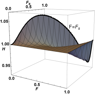
Figure 3: The function $H(r)\equiv\sqrt{-g}\sqrt{-M}$ is ploted in terms of $F$ and $F_{s}$. The solid black line defines the contour $F=F_{s}$.

Since the behaviour of $H(r)=\sqrt{-g}\sqrt{-M}$ is shown to be regular for all values of the relevant variables in Fig. 3 (see below for details of this and the next plots), from now on we will take $M^{\mu\nu}$ as the effective metric. For the Schwarzschild case we obtain

$$M^{tt} = \frac{F+\gamma[(1-6F+5F^{2})v-2Fv^{\prime}]}{F^{2}},$$ (40)

$$M^{rr} = \gamma v-F[1+\gamma v(3F-2)],$$ (41)

$$M^{\theta\theta} = -(F-1)^{2}[1+2\gamma v(F-1)-2\gamma v^{\prime}].$$ (42)

These expressions are a function of $r$ (through $F$, $v$ and $v^{\prime}$), and depend on the parameters $\gamma$ and $B$ (through $v$ and $v^{\prime}$). They can be rewritten in terms of $F_{s}$ and $F$ as follows . The constant $B$ can be expressed in terms of $\gamma$ and $F_{s}$ using the matching condition $(\psi_{+}-\psi_{-})|_{F_{s}}=0$. Now $\gamma$ can be written in terms of $F_{s}$ by use of the equation (III) evaluated at $F_{s}$, which yields a second order polinomial in $\gamma$. We choose to work with the negative root since $\gamma$ must be negative, as implied by the matching conditions (see Sect. III). We have then $\gamma=\gamma(F_{s})$, and $B=B(F_{s},\gamma(F_{s}))$. These two relations allow us to write the metric coefficients given above as functions of $F$ and $F_{s}$ only. We present in Figs. 4, 5, and 6 the plots of the metric coefficients for $F_{s}<F<1$. The solid black lines define the contours $F=F_{s}$. The plots show that each coefficient has the sign required to make the energy of the perturbations positive for any value of $F$ and $F_{s}$ in the relevant interval (that is, for any value of $\gamma<0$). Hence, we conclude that the system is linearly stable.

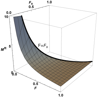
Figure 4: The metric coefficient $M^{tt}$ as a function of $F$ and $F_{s}$ for $F_{s}<F<1$. The solid black line defines the contour $F=F_{s}$.

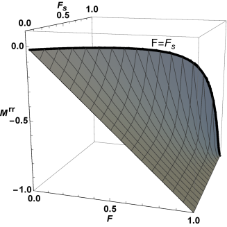
Figure 5: The metric coefficient $M^{rr}$ as a function of $F$ and $F_{s}$ for $F_{s}<F<1$. The solid black line defines the contour $F=F_{s}$.

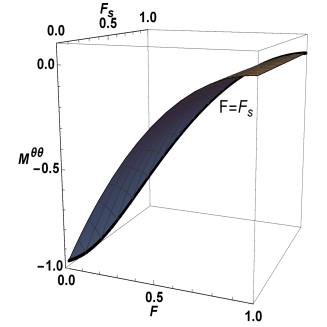
Figure 6: The metric coefficient $M^{\theta\theta}$ as a function of $F$ and $F_{s}$ for $F_{s}<F<1$. The solid black line defines the contour $F=F_{s}$.

V Conclusions

We have shown that the system composed of a Schwarzschild black hole accreting a steady-state and spherically symmetric galileon field described by the action given in Eqn.(1) is linearly stable using the method developed by Moncrief [15]. This method rests in the determination of the sign of the time derivative of the energy of the perturbations through a surface integral and leads in a few steps to the linear stability of any stationary solution of the system at hand that goes from being homogeneous at infinity, passes through a sonic horizon, and reaches the Schwarzschild horizon. The method profits from the symmetries of the system, and it does not use the explicit form of the solution for the scalar field. Extensions of this work, currently under way, are the study of the nonlinear stability of the system (since linear stability is only a prerequisite for full stability), and the determination of the stability of the accretion in the case of the model described by the combination of the first, second and fourth terms of the galileon Lagrangian.

References

- [1] Timothy Clifton, Pedro G. Ferreira, Antonio Padilla, and Constantinos Skordis. Modified Gravity and Cosmology. Phys. Rept., 513:1-189, 2012.
- [2] Alberto Nicolis, Riccardo Rattazzi, and Enrico Trincherini. The Galileon as a local modification of gravity. Phys. Rev., D79:064036, 2009.
- [3] C. Deffayet, Gilles Esposito-Farese, and A. Vikman. Covariant Galileon. Phys. Rev., D79:084003, 2009.
- [4] M. Ostrogradsky. Mémoires sur les équations différentielles, relatives au problème des isopérimètres. Mem. Acad. St. Petersbourg, 6(4):385-517, 1850.
- [5] A. I. Vainshtein. To the problem of nonvanishing gravitation mass. Phys. Lett., B39:393-394, 1972.
- [6] Eugeny Babichev and Cédric Deffayet. An introduction to the Vainshtein mechanism. Class. Quant. Grav., 30:184001, 2013.
- [7] E. Goulart and Santiago Esteban Perez Bergliaffa. Effective metric in nonlinear scalar field theories. Phys. Rev. D, 84:105027, 2011.
- [8] Javier Chagoya, Kazuya Koyama, Gustavo Niz, and Gianmassimo Tasinato. Galileons and strong gravity. JCAP, 1410(10):055, 2014.
- [9] Eugeny Babichev, Christos Charmousis, Antoine Lehébel, and Tetiana Moskalets. Black holes in a cubic Galileon universe. 2016.
- [10] Philippe Brax, Clare Burrage, and Anne-Christine Davis. Laboratory Tests of the Galileon. JCAP, 1109:020, 2011.
- [11] J. Neveu, V. Ruhlmann-Kleider, P. Astier, M. Besançon, J. Guy, A. Moller, and E. Babichev. Constraining the CDM and Galileon models with recent cosmological data. 2016.
- [12] Sourav Bhattacharya, Konstantinos F. Dialektopoulos, and Theodore N. Tomaras. Large scale structures and the cubic galileon model. JCAP, 1605(05):036, 2016.
- [13] Ayumu Terukina, Kazuhiro Yamamoto, Nobuhiro Okabe, Kyoko Matsushita, and Toru Sasaki. Testing a generalized cubic Galileon gravity model with the Coma Cluster. JCAP, 10:064, 2015.
- [14] E. Babichev. Galileon accretion. Phys. Rev., D83:024008, 2011.
- [15] V. Moncrief. Stability of stationary, spherical accretion onto a Schwarzschild black hole. Astrophys. J., 235:1038- 1046, February 1980.
- [16] Claudia A. Rivasplata Paz, Jose Martins Salim, and Santiago Esteban Perez Bergliaffa. Stability of the accretion of a ghost condensate onto a Schwarzschild black hole. Phys. Rev., D90(12):124075, 2014.
- [17] Patryk Mach and Edward Malec. Stability of relativistic Bondi accretion in Schwarzschild-(anti-)de Sitter spacetimes. Phys. Rev., D88(8):084055, 2013.
- [18] Carlos Barcelo, Stefano Liberati, and Matt Visser. Analogue gravity. Living Rev. Rel., 8:12, 2005. [Living Rev. Rel.14,3(2011)].